Article

A Physics-Informed, Machine Learning Emulator of a 2D Surface Water Model: What Temporal Networks and Simulation-Based Inference Can Help Us Learn about Hydrologic Processes

1
Department of Civil and Environmental Engineering, The High Meadows Environmental Institute and the Integrated GroundWater Modeling Center, Princeton University, Princeton, NJ 08544, USA
2
Department of Hydrology and Atmospheric Sciences, University of Arizona, Tucson, AZ 85721, USA
3
Department of Astrophysical Sciences and the Center for Statistics and Machine Learning, Princeton University, Princeton, NJ 08544, USA
*
Authors to whom correspondence should be addressed.
Water 2021, 13(24), 3633; https://doi.org/10.3390/w13243633
Submission received: 22 November 2021 / Revised: 12 December 2021 / Accepted: 13 December 2021 / Published: 17 December 2021

Abstract

:
While machine learning approaches are rapidly being applied to hydrologic problems, physics-informed approaches are still relatively rare. Many successful deep-learning applications have focused on point estimates of streamflow trained on stream gauge observations over time. While these approaches show promise for some applications, there is a need for distributed approaches that can produce accurate two-dimensional results of model states, such as ponded water depth. Here, we demonstrate a 2D emulator of the Tilted V catchment benchmark problem with solutions provided by the integrated hydrology model ParFlow. This emulator model can use 2D Convolution Neural Network (CNN), 3D CNN, and U-Net machine learning architectures and produces time-dependent spatial maps of ponded water depth from which hydrographs and other hydrologic quantities of interest may be derived. A comparison of different deep learning architectures and hyperparameters is presented with particular focus on approaches such as 3D CNN (that have a time-dependent learning component) and 2D CNN and U-Net approaches (that use only the current model state to predict the next state in time). In addition to testing model performance, we also use a simplified simulation based inference approach to evaluate the ability to calibrate the emulator to randomly selected simulations and the match between ML calibrated input parameters and underlying physics-based simulation.

1. Introduction

Hydrologic models are powerful tools that can represent processes and connections within the hydrologic cycle, facilitating both simulation and discovery [1]. Machine learning (ML) uses data-driven approaches to learn and then replicate a given behavior. ML approaches were first introduced to solve groundwater problems decades ago [2]. While discussion of these approaches in hydrology rapidly expanded [3,4], and adoption of these approaches has been increasing [5], there has been a strong focus on time-series prediction of streamflow at a gage.
Broadly, ML has shown great promise in the earth sciences [6], especially in the area of short-term streamflow and flood prediction [7,8]. However, the ability to use data-driven ML methods on their own to predict watershed behavior under changing conditions is limited by the decreasing relevance of historical data, sparse observations in the subsurface, and a lack of representative training samples [9,10]. As a result, there has been an increasing push for methods that can incorporate established theory into ML models (e.g., [11,12]). There are many emerging approaches to physics informed ML: augmenting physically-based models with ML, using theory to guide the ML models, or training ML emulators on physically based models [13]. After the initial training, such “emulators” can closely reproduce the simulation results at a fraction of the computational cost (e.g., [14,15,16,17]). Still, studies that develop ML-emulator models are rare in hydrology and hydrogeology. Recent examples include use of models to augment time observational datasets for streamflow prediction [18], learning subsurface constitutive relationships in variably-saturated systems [19,20], flood forecasting [21], and recent emulators of 3D hydrologic models [22].
Here, we develop a suite of ML-emulator models for a two-dimensional, time-dependent simulation of a benchmark surface-water catchment problem. We use a physically based hydrology model to provide training data for this ML emulator, which is trained using gridded pressure at the ground surface. In addition to demonstrating ML model performance, we test a range of ML architectures with a range of trainable parameters. We systematically test the impact training data quantity on ML model performance, the ability of the models to predict outside the range of input parameters, and the potential to calibrate the ML models to specific model configurations.

2. Materials and Methods

2.1. The Tilted V benchmark Problem

The Tilted V test problem [23,24,25,26] is an established benchmark used to test hydrologic models [
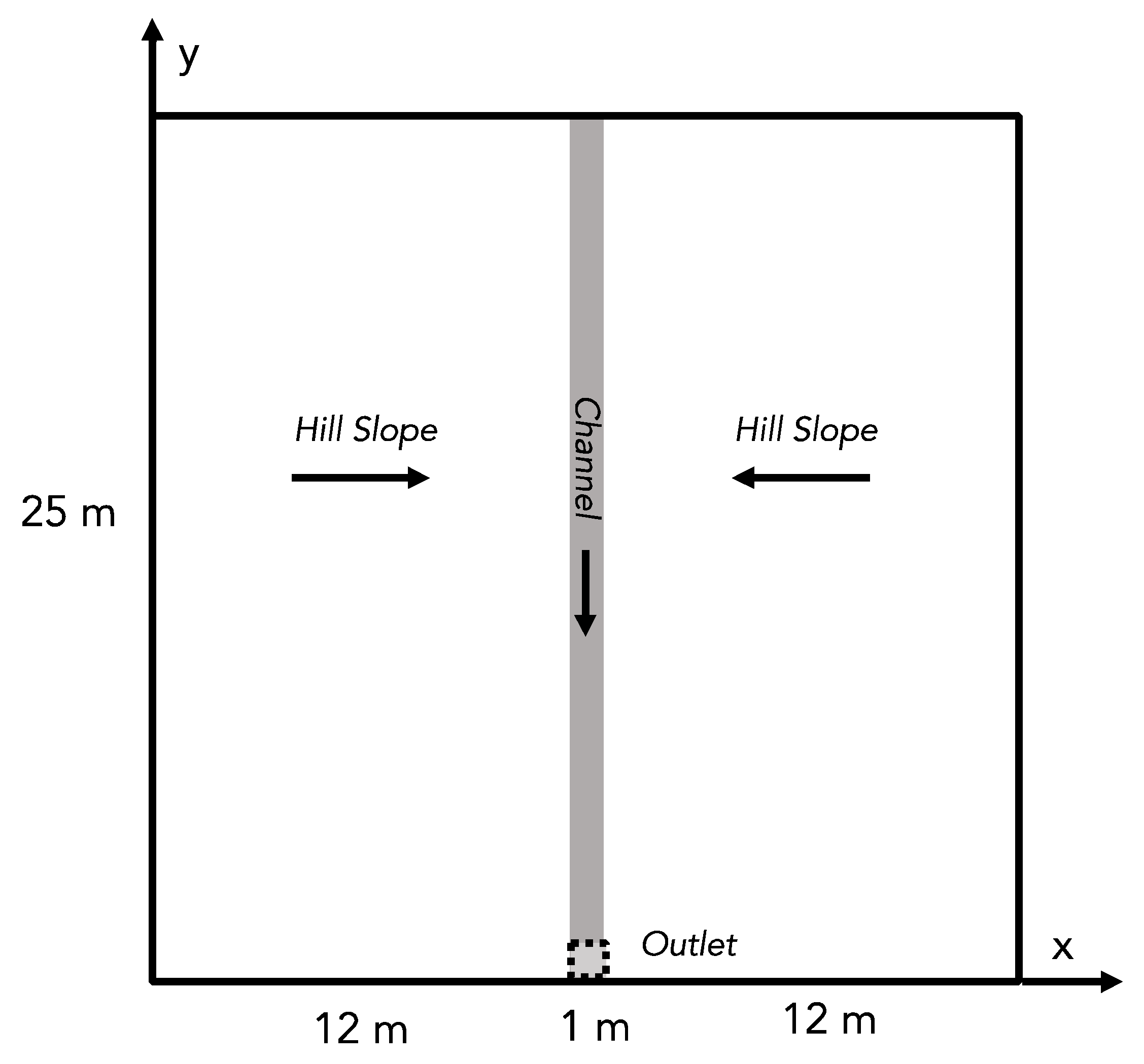
27]. This test problem is shown in Figure 1 and is one of the simplest representations of a watershed shape. The problem domain is square and contains two hillslopes that drain inward to a central channel. The entire domain is then sloped along the channel (the y-direction in Figure 1), usually with a shallower channel slope than the hillslopes. Though there are different variations, generally, the domain is initialized dry and rained on for a given duration after which there is a period of recession. The total flow for the domain is usually calculated at the outlet of the channel, shown in Figure 1. This test problem is solved with the surface water equations.
The surface water equations [27] combine the continuity equation and the Manning’s depth-discharge relationship in two spatial dimensions as follows:
h t = · ( v h ) + q r a i n
where h is the pressure head (m), qrain is the rainfall flux (mh−1), t is time (h), and v is the velocity given by the depth-discharge relationship:
v x , y = S x , y h 2 3 n
Sx,y are the topographic slopes in the x and y directions (-), and n is the Manning’s roughness coefficient (m1/3h−1). There are many approaches to solving for surface water flow; however, no analytical solutions exist for the Tilted V test problem. In this work, the integrated hydrologic model ParFlow [26,28,29] was used to solve these equations.

2.2. Numerical Solution of the Tilted V and General Training Approach

The integrated hydrologic model ParFlow [
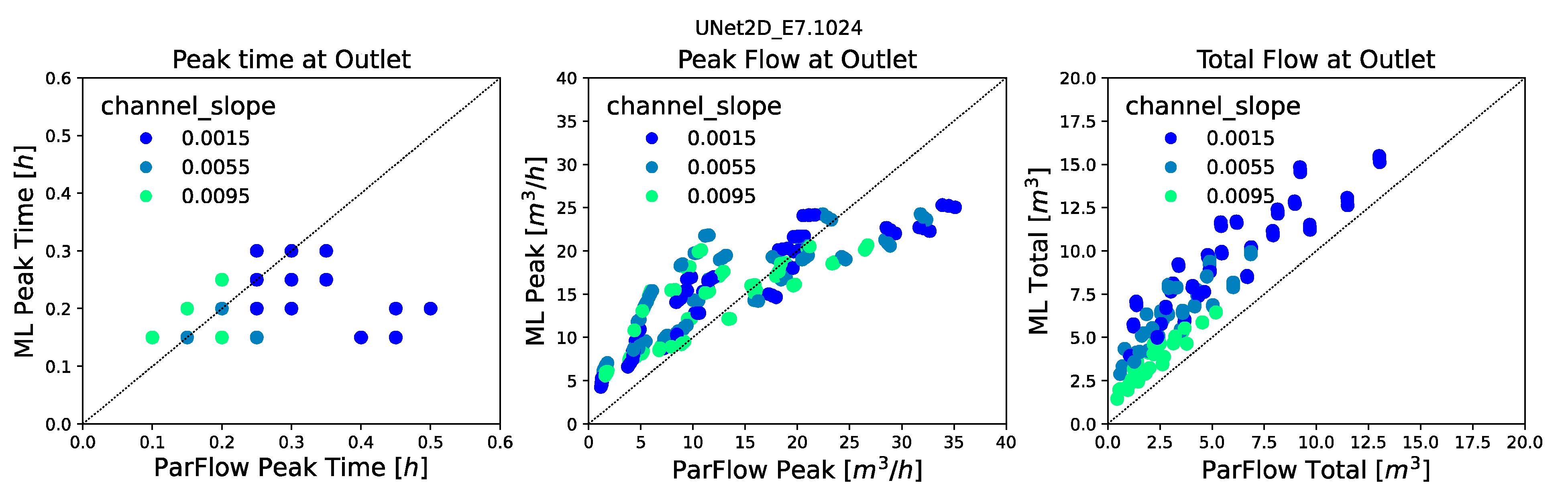
30] was used to solve the 2D overland flow equations for the Tilted V benchmark problem. Model input parameters were systematically varied across a range of values to generate a suite of ensemble simulations (Table 1). Three sets of simulations were conducted with ParFlow: a 1024-member ensemble used to train the ML models and two test ensembles with 243 and 32 ensemble members, respectively. One of the two test datasets was constructed to have same parameter ranges as the training dataset (In Range), while the other was constructed to have parameters outside the range used for training (Full Range).
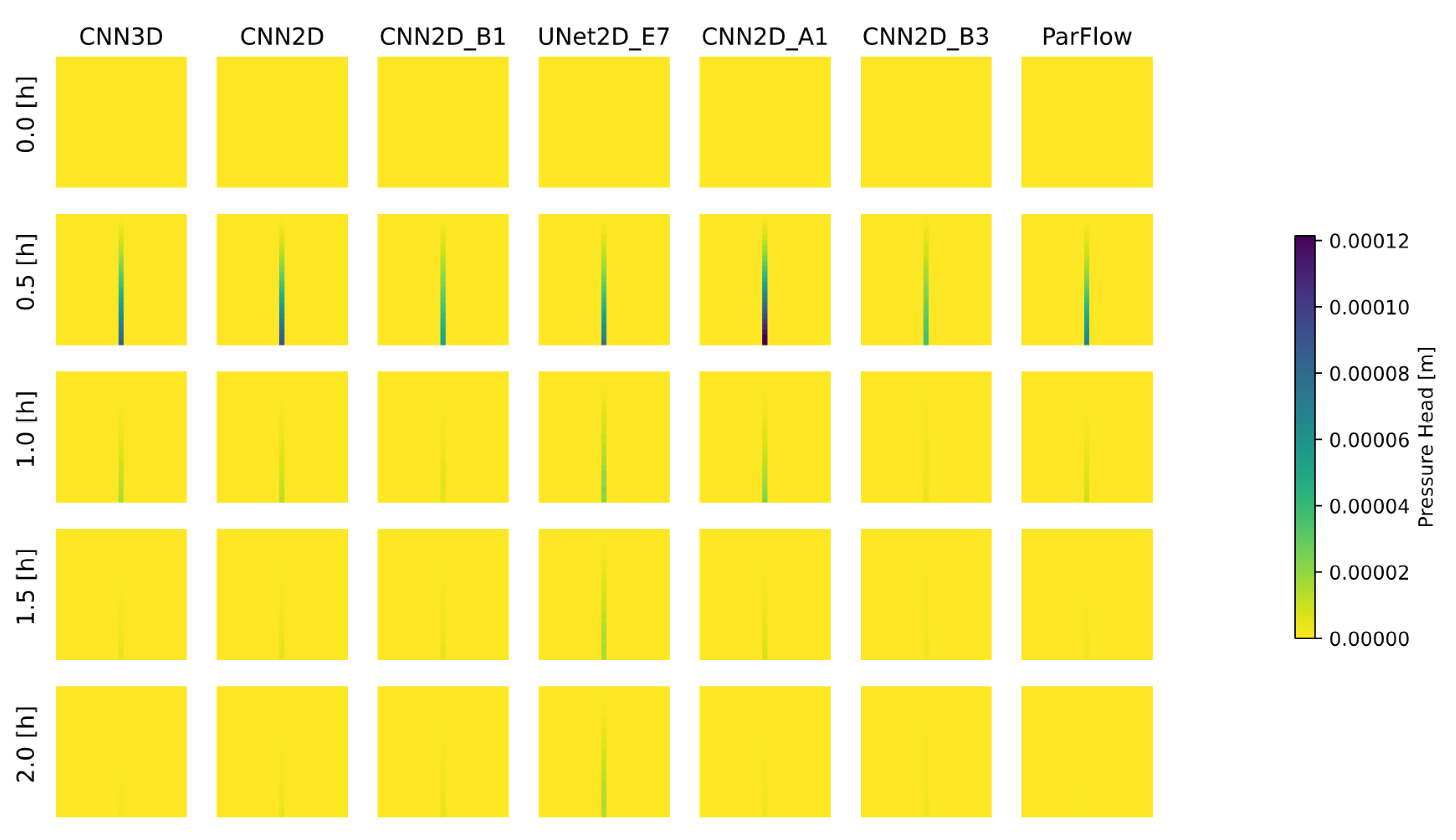
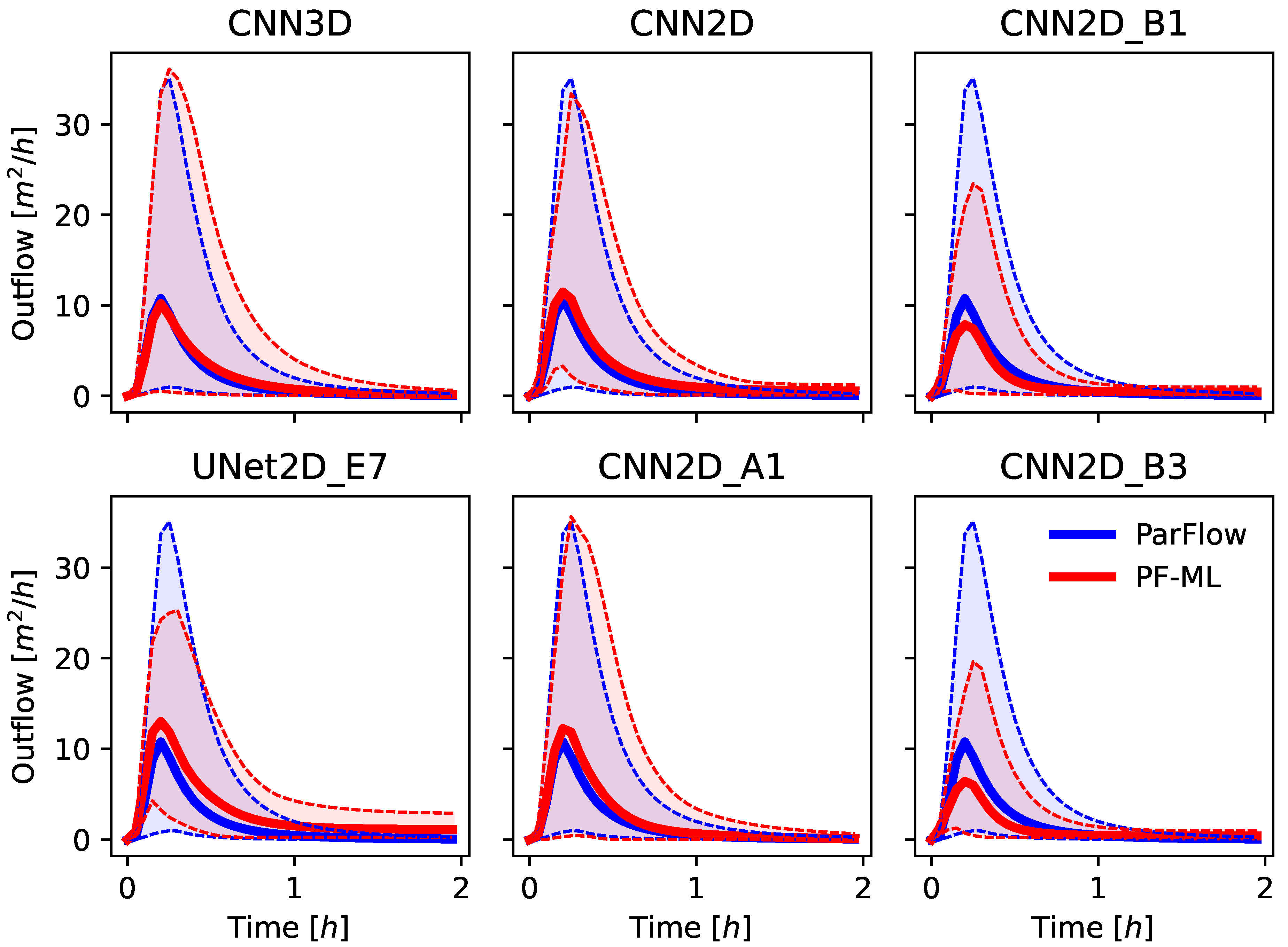
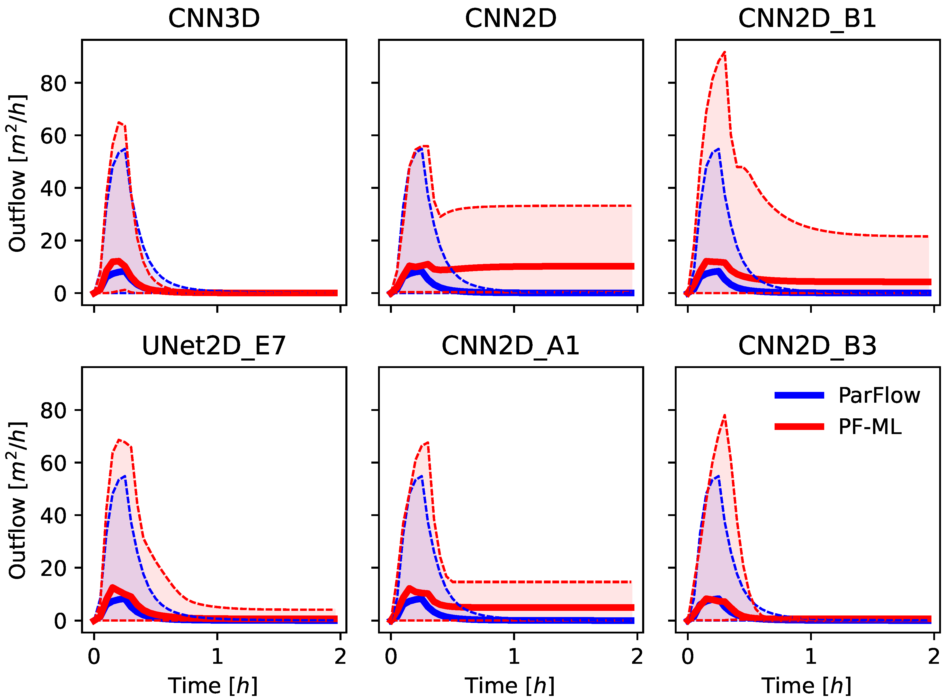
The solution for both ParFlow and the ML-emulator models results in a 2D time-dependent map of pressure-head over the domain, which represents the height of ponded water above the ground surface. Most solutions to the Tilted V then calculate the hydrograph at the outlet (discussed above) using Manning’s Equation (Equation (2)) with the surface pressure at the outlet cell as input. This same approach was used for the ML-emulator models as well. Specifically, only the surface pressure was used in the loss function during training, not the outflow hydrograph from the ParFlow simulations. This is in contrast to prior ML approaches that might focus on learning the hydrograph directly [3,5]. This approach is more general and allows for the ML model to produce other hydrologic quantities that could be of interest for, e.g., flooding or water management; however, the hydrographs produced are very sensitive to the convergence of the surface pressure.

2.3. ML Model Architectures

We chose several machine learning architectures from which to construct emulator model of the Titled V problem. Six ML models were chosen to be described in the experiments presented here from a trial-and-error process that involved over 30 different emulators. Because the focus here is on reproducing the change in a 2D grid of values over time, we developed models based upon the Convolution Neural Net (CNN) architectures [31,32] commonly used in video reconstruction and extrapolation [33]. We also applied U-Net approaches, which are better suited for maintaining spatial information [34]. The ML models used in this study were chosen to represent three main architectures (2D CNN, 3D CNN, and U-Net) with a varying degree of depth, as indicated by the total number of parameters. The 3D model was designed to be trained on temporal behavior of the system explicitly and simulates the entire timeseries at once, while the 2D models are designed to simulate only one timestep at a time. Complete details of the models developed for this study are provided in Appendix A, and the models are summarized as follows:
  • CNN3D, a deep 3D convolution (third dimension is time) detailed in Table A1;
  • CNN2D, a deep 2D convolution detailed in Table A2;
  • CNN2D_B1, a moderately deep 2D convolution detailed in Table A3;
  • UNet2D_E7, a three-level U-Net detailed in Table A4;
  • CNN2D_A1, a deep 2D convolution with no pooling detailed in Table A5; and
  • CNN2D_B3, a very shallow 2D convolution detailed in Table A6.
The CNN3D model had the most parameters (>240M), while the CNN2D_B3 model had the least (83K). The CNN2D model is quite similar in architecture and size to the CNN3D but, as noted above, is not explicitly trained on the time series of the simulation results. The CNN2D and CNN2D_A1 models are similar in size and architecture except that the CNN2D_A1 model has no pooling steps, only convolutions. The models were all implemented using the Pytorch Python library [35]. Numerical experiments and training details are provided in the following section.

2.4. ML Model Training

As shown in Table 1, the channel and hill slopes were varied (see Figure 1) to construct 2D slope inputs (in x and y); the Manning’s roughness value was uniform over the domain and varied across the values as given. The given rain rate, start, and length were used to create a time series of rainfall inputs. A training dataset and two independent test datasets were developed as indicated.
Table 1. Tilted V test case, training, and test parameters.
Training Test In Range Test Full Range
VariableUnitsLowerMid1Mid2UpperLowerMidUpperLowerUpper
channel slope(-)0.0010.0040.0070.010.00150.00550.00950.010.02
hill slopes(-)0.050.0830.1170.150.0550.07750.10.010.2
Manning’s n(m1/3h−1)8.3 × 10−68.8 × 10−69.3 × 10−69.7 × 10−68.5 × 10−68.8 × 10−69.0 × 10−65.0 × 10−62.1 × 10⁻⁵
rain rate(mh−1)−0.005−0.01−0.015−0.02−0.007−0.011−0.015−0.004−0.02
rain start(h)000000000
rain length(h)0.10.150.20.250.10.150.250.10.3
These were all fed into the ML models as static (Sx, Sy, n) or time-dependent (rainfall) two-dimensional fields that corresponded to the grid. That is, instead of using a single-channel slope or rainfall value as input, a full 2D map was constructed, even for variables like the Manning’s n, which were constant in space. This was done to allow the framework to accommodate heterogeneity in parameter values in future studies. All models had the same domain configuration, where nx = ny = 25 with ∆x = ∆y = 1 [m]. All models were also run for a total time of two hours with forty uniform timesteps, ∆t = 0.05 [h].
All six of the ML models were trained on the training ensemble (detailed below) using a Nvidia 2080 Super Max-Q GPU. The learning rate was set to 10−4 using the Adam optimizer [36], with 2500 epochs of training for each case. A Smooth L1 loss function was calculated between the ML-predicted pressure field and the field produced by the ParFlow simulation at each snapshot in time. Only two hyperparameters (learning rate and number of epochs) were chosen through experimentation on the training data. Note that other hyperparameters in the models themselves (e.g., number of output channels, size of the linear layer) were not tuned but vary between model simulations in the experiments presented here. The final loss values for all models was below 10−4, with some being below 10−5. Training times were not rigorously tracked but ranged from approximately 2 min for the 2DCNN_B3 model to about an hour for the U-Net.
The base case simulations used all 1024 training realizations for training, while some models were also trained with a reduced set of training realizations chosen at random (512, 256, 128, 64, and 32) to test the sensitivity of the trained model to size of the input data. This process is similar in principle to an Ablation Study [37] except that here, the number of realizations systematically removed some of the training input rather than systematically removing components of the ML model. This resulted in 27 total model simulations, as shown in Table 2. Hereafter, these models will be referred to by the model name and the number of realizations; e.g., CNN3D.1024 would be the three-dimensional CNN trained on all 1024 of the ParFlow Tilted V simulations.
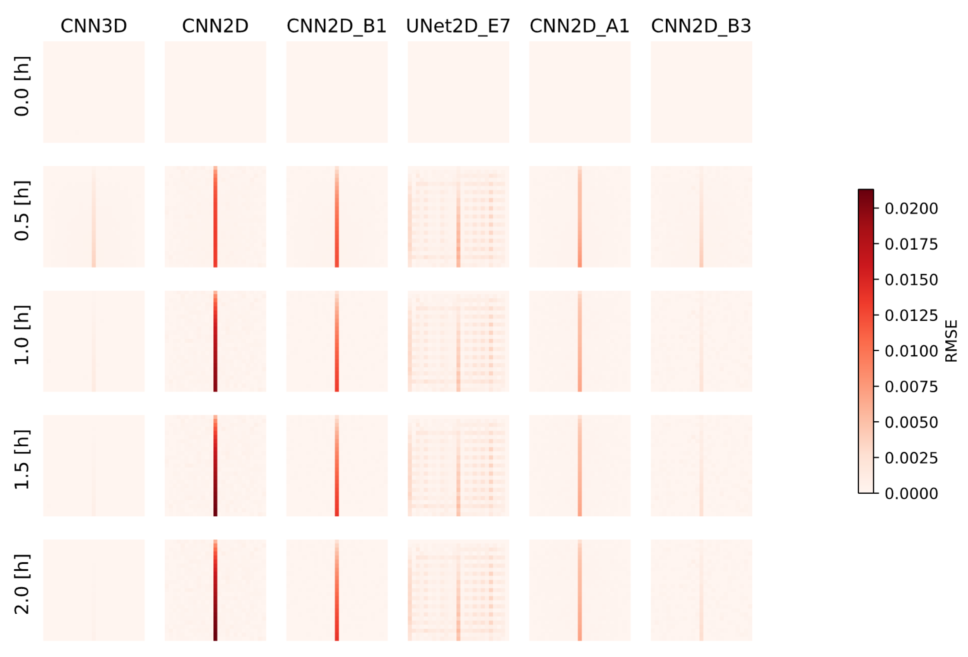
Several model evaluation metrics were used in this study to assess ML model performance both for the spatially distributed outputs and the calculated hydrographs. These include the Root Mean Squared Error (RMSE) of the pressure fields and of the calculated hydrographs, the Pearson’s Correlation Coefficient (commonly the R2 statistic), and Spearman’s Rank Correlation Coefficient (commonly the Spearman’s Rho) of the ML predicted and ParFlow simulated hydrographs. These metrics were calculated for each realization in the ensemble, and the mean and variance were reported across the test ensembles.

2.5. Parameter Evaluation

Finally, we evaluated whether the ML simulations can match the parameters of the model ParFlow in addition to the outputs (i.e., if our ML models get the right answer for the right reasons). Model calibration or parameter estimation is widely used in the hydrologic sciences (e.g., [38]). Simulation Based Inference (SBI, see, e.g., Cranmer et al. [39]) is somewhat different than traditional calibration. Briefly, SBI compares the simulation outputs to observations to infer the likelihood of a particular parameter set given some observations. Simulations are used to define the relationship between parameters and target variables in cases where a conventional likelihood evaluation is either theoretically or practically infeasible.
Here, we do not apply full SBI; rather, we tested whether our trained emulator models are able to match the parameters of the underlying simulations and not just their outputs. For this test, we used three of the trained emulator models (CNN2D.1024, UNet2D.1024, and CNN2D_B3.1024) using the following a procedure that resembles Approximate Bayesian Computation (ABC, [40]):
  • Three ParFlow simulations were selected at random from the In Range ensemble and their hydrographs calculated, and these are defined as our target ParFlow “truth” simulations;
  • A full suite of simulations were conducted with the three ML models varying parameters shown in Table 1 across the complete set of In Range ensemble values;
  • Hydrographs were calculated from the entire suite of the ML models, and the RMSE was calculated for every realization compared to each of the ParFlow “truth” simulations;
  • The five realizations with the lowest RMSE values were selected as the best performing ML realizations;
  • The parameters for the best-matching ML realizations were compared to the parameters from the ParFlow “truth” simulations to evaluate whether the emulators would preserve the behavior of the ParFlow parameters.
This analysis is not intended to be a formal SBI or model calibration; rather, the purpose is to further explore the validity of our emulators. This approach is much more simple than other calibration approaches that might employ an evolution search algorithm [41], gradient-based method to adjust parameters in a series of more limited model simulations [42] or even use ML approaches to replace the calibration routine [43]. Given this proof of concept, future work should include more complex frameworks, including those that loop parameters back to the original physical model simulation or use a more formalized Bayesian framework [44].

3. Results and Discussion

The results are organized as follows: first a baseline model test is presented (3.1); then, model sensitivity to training data explored (3.2); next, the models are tested on simulations outside the parameter range used in training (3.3); and finally, the results of ABC are presented and discussed (3.4).

3.1. Base-Case Model Performance and In Range Test Cases

The surface pressure (h in Equation (1)) for the base case trained ML models (described in Table 2) were compared to the corresponding ParFlow simulated pressures. This was done for the average over the entire In Range test simulations (Figure 2) and the RMSE between every simulated timestep of pressure and ParFlow (Figure 3). In Figure 2, we see that all models represent the basic spatial and temporal patterns simulated by ParFlow, with high pressures occurring along the central channel of the domain where water accumulates and flows to the exit. This behavior is similar in general to the results of prior flood mapping studies [21] and other emulator studies [22]. Visually, the CNN3D and CNN2D cases appear to have the closest average behavior to that simulated by ParFlow. The UNet2D_E7 model represents the timing behavior the most poorly, with greater channel pressures later in the simulation. The CNN2D_B3 model also misrepresents the timing with pressures decreasing in the channel too quickly. The RMSE maps (Figure 3) confirm this, with the largest mismatches occurring in the channel for these two models at later times. The UNet2D_E7 model also demonstrates a mismatch in the right hillslope, while the other models appear to represent the hillslope values well.
Hydrographs for all the base case models were calculated (Equation (2)) at the outlet location shown in Figure 1. These hydrographs were then compared to the ParFlow simulations for all realizations of the In Range ensemble. Figure 4 plots the envelope of all hydrographs as a function of time, and the average is shown as a solid line (blue for ParFlow, red for the ML models) and a shaded region that encompasses the entire distribution. Recall that the hydrographs are not used in training, nor is the ML model given any input that attaches specific significance to that location. In general, we see a good match between the hydrographs produced by the ML models and those produced by ParFlow. This finding is similar to results of another emulator study [22]. Visually, the CNN3D model has the best match to the simulated hydrographs, with the CNN2D_A1 and CNN2D models also exhibiting a good fit. This result is somewhat surprising given that the CNN2D_A1 model excludes pooling (see Table A5). The UNet2D_E7 and shallower CNN2D_B1 and CNN2D_B3 models do not represent the entire ensemble spread. Closer inspection reveals that this is due to the timing issues discussed above; the UNet2D_E7 model overestimates the hydrograph tail, while the CNN2D_B3 and CNN2D_B1 models underestimate it.

3.2. Model Sensitivity to Training Data

The heat maps in Figure 5 display metrics of performance for the complete suite of the 27 models given in Table 2. This table presents the Pearson Correlation Coefficient, Spearman’s Rho, and RMSE calculated across the hydrographs for the In Range test set presented as a mean and a variance over the ensemble. This figure is colored such that blue colors indicate a better metric of agreement or a lower error or standard deviation. This figure again confirms that the CNN3D model exhibited the best performance, closely followed by the deeper 2D CNN models, CNN2D, and CNN2D_A1. The models do not perform uniformly across all metrics; while the performance of the UNet2D.1024 model is like the CNN2D.1024 and CNN2D_A1.1024 in Pearson and Spearman, it has a larger RMSE. We also see that the UNet2D_E7.128 and UNet_E7.32 models do not perform as well as the other models.
As training data are systematically ablated, the model performance does not uniformly decrease. Figure 5 includes metrics for this aspect of our study. The CNN3D model performs the best across this reduction in training data, and the CNN 2D_A1 also performs well. We see that shallower CNN2D_B3 and CNN2D_B1 models do not perform as well as the deeper models with fewer training realizations. However, the results of this study show that, in general, good model performance is achieved with fewer realizations, which saves both physical model-simulation time and ML model-training expense.
Figure 5. Heatmap for three metrics (Pearson Correlation Coefficient, Spearman’s Rho, and RMSE) calculated for the hydrographs derived from all ML simulations compared to ParFlow across all 243 In Range test realizations. As indicated in the titles, the ensemble mean of each metric is shown in the top row, and the standard deviation of each metric is shown in the bottom row. Models were trained on a different number of realizations, as indicated by the x-axis in each subplot.
Water 13 03633 g005
The models exhibited a different ability to represent three hydrograph features: peak hydrograph timing, peak hydrograph flow, and the total flow. Scatterplots of these three features are shown in Figures 8–10, for the CNN3D.1024, CNN2D.1024, and UNet2D.1024 models, respectively, compared to ParFlow, for the In Range test set. Of the three models, the CNN3D.1024 represents the peak hydrograph behavior the best, with both the peak timing and flow matching ParFlow well (Figure 6). The CNN2D.104 exhibited better total flow (Figure 7) than the CNN3D.1024 model although it had trouble representing cases with later peak timing. Figure 8 further emphasizes the later timing predicted by the UNet2D.1024 model. Figure 6, Figure 7 and Figure 8 are colored by the channel slope, and generally lower values of channel slope are associated with a poorer match for peak timing and total flow in Figure 6 and Figure 7. Overall, the models appear to be challenged by combinations of lower channel slope and higher precipitation values. This might be a structural feature in the models themselves or an indication that the training might be better designed to emphasize these values more. That is, instead of being uniform over the entire input range, training might be better if an additional number of low-slope cases were included in the ensemble in a reinforcement-learning-type approach.

3.3. Full Range Test Cases

The trained ML models were also compared to ParFlow simulations for the Full Range test set described in Table 1 (recall that the Full Range ensemble includes parameter values that fall outside the parameter range used for training). These results are shown for average pressure over five snapshots in time in Figure 9. Visually, all the ML models show some degraded performance with input parameters that are outside of the training dataset. The UNet2D_E7 model shows the poorest average performance, with large artifacts occurring in the hillslopes. The 2D CNN models also show degraded performance in the hillslopes, exhibiting random noise. The RMSE of pressure for these simulations (Figure 10) further emphasize these misfits between ML model and ParFlow results. The CNN3D model has the best overall match, and other models (e.g., CNN2D) start to exhibit more temporal mismatch when simulations fall outside the training range.
Figure 9. Surface pressure averaged across all 32 Full Range test realizations for the six ML models compared to the ParFlow simulations, at five snapshots in time. All models were trained on 1024 realizations.
Water 13 03633 g009
Figure 10. RMSE of surface pressure between each of the six ML models and ParFlow simulations calculated across all 32 Full Range test realizations, at five snapshots in time. All models were trained on 1024 realizations.
Water 13 03633 g010
Figure 11 plots the calculated hydrographs for each base case in the same manner as in Figure 4 but now for the Full Range test set. While all models produce hydrographs that match more poorly than those in Figure 4, the CNN3D case still has reasonable performance. Some of the 2D CNN models (CNN2D, CNN2D_B1) have realizations that blow up and produce very unrealistic behavior, while others (CNN2D_A1) exhibit more systematic biases, such as overpredicting timing of the recession. While these results generally confirm that ML models can most reliably predict events in their training history, some models do learn behavior that translates outside the range of the input data.
Figure 11. Ensemble hydrograph comparisons between each of the six ML models and ParFlow simulations across all 32 Full Range test realizations. The ensemble mean is shown for both ML (red) and ParFlow (blue) along with a shaded range that represents the entire spread across all ensemble members. All models were trained on 1024 realizations.
Water 13 03633 g011

3.4. Parameter Evaluation

As detailed in Section 2.5, we completed set of realizations for the entire In Range parameter set using three ML models. We then selected the five ML realizations for each model that most closely match a randomly selected ParFlow “truth” simulations by minimizing the RMSE between ML and ParFlow hydrographs. First, we note that the ML architectures are all able to produce hydrographs that closely match our randomly selected “truth” realizations (Figure 12 and Figure 13). This is true even for ML models such as CNN2D_B3 and UNet2D_E7, which exhibited poorer base-case performance. The five CNN2D model hydrographs bracketed the “true” ParFlow hydrograph in all three cases although none of the realizations themselves were a perfect match (Figure 12). The CNN2D_B3 model was unable to completely capture two of the ParFlow realizations due to high peak flow value, which was not captured by any realization in its ensemble (Figure 13). The UNet2D_E7 model was also able to bracket all three hydrographs (not shown). Overall, these results are promising and demonstrate the ability for the ML simulations to be tuned to match observations with.
Next, we explored whether the parameters from the selected best realizations also agree with the original ParFlow simulation. Recall that the best ML realizations were selected purely based on the RMSE of the hydrographs and not parameter matching. Therefore, evaluating whether the parameters for the selected realizations also match the ParFlow simulations is a good indication that the ML models are getting the right answer for the right reasons and have learned relationships between model parameters and outputs that match the information embedded in our Physics based model, ParFlow.
To evaluate parameter match, we calculated a Normalized RMSE (NRMSE) score for each of our input parameters. This NRMSE was calculated as the difference between each parameter estimate and the true parameter divided by the true parameter value. Normalizing by the true parameter value allows us to compare fit across parameters with different values and ranges in the ensemble inputs (see Table 1). As an example, Table 3 lists the parameter values for each of the top five realizations for the CNN2D model, the ParFlow truth model, and the NMRSE between them. This table shows that, in most cases, the five ML parameter sets are either the same or bracket the true ParFlow parameters. This provides further confidence in our results, suggesting that our ML models have learned relationships between input parameters and streamflow that match the relationships of the underlying model.
The NRMSE was calculated for the five input parameters of the five closest realizations for all three of the ML models tested (CNN2D.1024, CNN2D_B3, and UNet2D_7). Histograms of these 75 NRMSE values are plotted for in Figure 14. The mean NRMSE values were lowest for the CNN2D.1024 model (0.29), second lowest for the CNN2D_B3.1024 model (0.43), and largest for the UNet2D_E7 model (0.86). Both the CNN2D_B3.1024 and the UNet2D_E7.1024 models display a large range of NRMSE values. The UNet2D_E7 model fits the three ParFlow simulations well yet has the largest NRMSE values, indicating that there is some bias in the underlying ML model. The best CNN2D.1024 realizations have parameter values that are closer to the original ParFlow model than the other two models. These results highlight both the challenges of non-uniqueness in our ML simulations but also the potential for the model architectures to learn correct parameter behaviors.

4. Conclusions

This manuscript describes the development of a ML-emulator model of a common hydrologic benchmark problem trained on the output from the numerical platform, ParFlow. A range of ML architectures were successfully trained and tested on test datasets that were within and outside the parameter ranges of the training data. Additionally, we used an ABC framework to demonstrate that the ML models can be successfully calibrated. Several distinct conclusions can be drawn from this work.
  • ML models can be trained as general emulators of hydrologic behavior. ML models that are given the same input data and are run in the same manner as a physical hydrologic model (e.g., CNN2D) are possible and still exhibit good performance across a range of metrics. They can be given the same input as a physically based hydrologic model and produce the same outputs, in this case, time-dependent maps of surface pressure. This is exciting and suggests that true ML-emulator models for more complex problems are also possible.
  • This is a distinctly new approach to applications of ML in hydrology and suggests that a ML model can learn general physical behavior.
  • ML models that were provided with explicit temporal information during training (CNN3D) showed the best performance across a range of metrics. This suggests that the ML models without explicit temporal dependence do not contain the ability to simulate underlying hydrologic processes the same as the physically based model. The physical processes represented by hydrologic models allow them to convert spatial patterns in pressure to temporal behavior at the outlet. For best performance, ML models should be trained on time series to emulate the dynamics of hydrologic models.
  • Deeper networks (CNN3D, CNN2D) perform better than models with fewer parameters (CNN2D_B1, CNN2D_B3). Some hydrograph metrics, such as total flow, are easier for the models to capture, while others, such as peak timing, are more challenging.
  • ML-emulator models perform best when tested on cases with inputs that fall within the range of the parameter sets used for training. While some of the deeper models (CNN3D) exhibited good performance for the Full Range test set, other models exhibited very poor and even unrealistic behavior.
  • We demonstrate that ML models can be successfully calibrated using an ABC approach. This approach calibrated the parameters of the ML model directly on a synthetic observation. We found that this approach could consistently improve model performance. Moreover, in many cases, the resulting calibrated model parameter sets correlated well with the original ParFlow inputs, indicating a good match between the learned model behaviors and ParFlow relationships between parameters and simulated outputs.
While this work was undertaken on a synthetic, benchmark test case for a single rain event, it represents an important proof of concept. This simulation framework can easily be extrapolated to real domains with real forcing.

Author Contributions

Conceptualization, R.M.M., L.E.C. and P.M.; Methodology, R.M.M., L.E.C. and P.M., Software, R.M.M. and L.E.C.; Writing—Original Draft Preparation, R.M.M. and L.E.C.; Writing—Review & Editing, R.M.M., L.E.C. and P.M.; Funding Acquisition, R.M.M., L.E.C. and P.M. All authors have read and agreed to the published version of the manuscript.

Funding

This research was funded by the US National Science Foundation Convergence Accelerator Program, grant number CA-2040542.

Data Availability Statement

The ParFlow model is available at https://github.com/parflow, example ML model workflows are available at https://github.com/HydroGEN-pubs/TV-ML, and the underlying ParFlow model simulations are available at https://github.com/HydroGEN-pubs/TiltedV-2D.

Conflicts of Interest

The authors declare no conflict of interest.

Appendix A. Detailed Tables of the ML Model Architectures

The six tables below provide detailed information on each of the ML models used in this work. Each table presents the model layers in order, along with the associated shape and number of parameters. A summary value for the total number of trainable parameters is given for each model.
Table A1. ML structure, shape, and parameters for CNN3D.
Layer Output ShapeNumber of Parameters
├─Sequential: 1-1[18, 10, 6, 6]
│  └─Conv3d: 2-1[18, 40, 25, 25]2448
│  └─ReLU: 2-2[18, 40, 25, 25]
│  └─Conv3d: 2-3[18, 40, 25, 25]8766
│  └─ReLU: 2-4[18, 40, 25, 25]
│  └─MaxPool3d: 2-5[18, 20, 12, 12]
│  └─Conv3d: 2-6[18, 20, 12, 12]8766
│  └─ReLU: 2-7[18, 20, 12, 12]
│  └─MaxPool3d: 2-8[18, 10, 6, 6]
├─Linear: 1-2[7000]45,367,000
├─Linear: 1-3[25,000]175,025,000
Total:220,411,980
Table A2. ML structure, shape, and parameters for CNN2D.
LayerOutput ShapeNumber of Parameters
├─Sequential: 1-1[18, 6, 6]
│  └─Conv2d: 2-1[18, 25, 25]828
│  └─ReLU: 2-2[18, 25, 25]
│  └─Conv2d: 2-3[18, 25, 25]2934
│  └─ReLU: 2-4[18, 25, 25]
│  └─MaxPool2d: 2-5[18, 12, 12]
│  └─Conv2d: 2-6[18, 12, 12]2934
│  └─ReLU: 2-7[18, 12, 12]
│  └─MaxPool2d: 2-8[18, 6, 6]
├─Linear: 1-2[20,000]12,980,000
├─Linear: 1-3[625]12,500,625
Total:25,487,321
Table A3. ML structure, shape, and parameters for CNN2D_B1.
LayerOutput ShapeNumber of Parameters
├─Sequential: 1-1[6, 6, 6]
│  └─Conv2d: 2-1[6, 25, 25]276
│  └─ReLU: 2-2[6, 25, 25]
│  └─MaxPool2d: 2-3[6, 12, 12]
│  └─Conv2d: 2-4[6, 12, 12]330
│  └─ReLU: 2-5[6, 12, 12]
│  └─MaxPool2d: 2-6[6, 6, 6]
├─Linear: 1-2[7000]1,519,000
├─Linear: 1-3[625]4,375,625
Total:5,895,231
Table A4. ML structure, shape, and parameters for UNet2D_E7.
LayerOutput ShapeNumber of Parameters
├─Sequential: 1-1[16, 12, 12]
│  └─Conv2d: 2-1[16, 25, 25]736
│  └─BatchNorm2d: 2-2[16, 25, 25]32
│  └─ReLU: 2-3[16, 25, 25]
│  └─Conv2d: 2-4[16, 25, 25]2320
│  └─BatchNorm2d: 2-5[16, 25, 25]32
│  └─ReLU: 2-6[16, 25, 25]
│  └─MaxPool2d: 2-7[16, 12, 12]
├─Sequential: 1-2[32, 6, 6]
│  └─Conv2d: 2-8[32, 12, 12]4640
│  └─BatchNorm2d: 2-9[32, 12, 12]64
│  └─ReLU: 2-10[32, 12, 12]
│  └─Conv2d: 2-11[32, 12, 12]9248
│  └─BatchNorm2d: 2-12[32, 12, 12]64
│  └─ReLU: 2-13[32, 12, 12]
│  └─MaxPool2d: 2-14[32, 6, 6]
├─Sequential: 1-3[64, 3, 3]
│  └─Conv2d: 2-15[64, 6, 6]18,496
│  └─BatchNorm2d: 2-16[64, 6, 6]128
│  └─ReLU: 2-17[64, 6, 6]
│  └─Conv2d: 2-18[64, 6, 6]36,928
│  └─BatchNorm2d: 2-19[64, 6, 6]128
│  └─ReLU: 2-20[64, 6, 6]
│  └─MaxPool2d: 2-21[64, 3, 3]
├─Sequential: 1-4[32, 6, 6]
│  └─Conv2d: 2-22[32, 3, 3]18,464
│  └─BatchNorm2d: 2-23[32, 3, 3]64
│  └─ReLU: 2-24[32, 3, 3]
│  └─Conv2d: 2-25[32, 3, 3]9248
│  └─BatchNorm2d: 2-26[32, 3, 3]64
│  └─ReLU: 2-27[32, 3, 3]
│  └─ConvTranspose2d: 2-28[32, 6, 6]4128
├─Sequential: 1-5[16, 12, 12]
│  └─Conv2d: 2-29[32, 6, 6]18,464
│  └─BatchNorm2d: 2-30[32, 6, 6]64
│  └─ReLU: 2-31[32, 6, 6]
│  └─Conv2d: 2-32[16, 6, 6]4624
│  └─BatchNorm2d: 2-33[16, 6, 6]32
│  └─ReLU: 2-34[16, 6, 6]
│  └─ConvTranspose2d: 2-35[16, 12, 12]1040
├─Sequential: 1-6[1, 25, 25]
│  └─Conv2d: 2-36[32, 12, 12]9248
│  └─BatchNorm2d: 2-37[32, 12, 12]64
│  └─ReLU: 2-38[32, 12, 12]
│  └─Conv2d: 2-39[16, 12, 12]4624
│  └─BatchNorm2d: 2-40[16, 12, 12]32
│  └─ReLU: 2-41[16, 12, 12]
│  └─ConvTranspose2d: 2-42[1, 25, 25]65
Total:143,041
Table A5. ML structure, shape, and parameters for CNN2D_A1.
LayerOutput ShapeNumber of Parameters
├─Sequential: 1-1[16, 25, 25]
│  └─Conv2d: 2-1[16, 25, 25]736
│  └─ReLU: 2-2[16, 25, 25]
│  └─Conv2d: 2-3[16, 25, 25]2320
│  └─ReLU: 2-4[16, 25, 25]
│  └─Conv2d: 2-5[16, 25, 25]2320
│  └─ReLU: 2-6[16, 25, 25]
├─Linear: 1-2[7000]70,007,000
├─Linear: 1-3[625]4,375,625
Total:74,388,001
Table A6. ML structure, shape, and parameters for CNN2D_B3.
LayerOutput ShapeNumber of Parameters
├─Sequential: 1-1[5, 6, 6]
│  └─Conv2d: 2-1[5, 25, 25]230
│  └─ReLU: 2-2[5, 25, 25]
│  └─MaxPool2d: 2-3[5, 12, 12]
│  └─Conv2d: 2-4[5, 12, 12]230
│  └─ReLU: 2-5[5, 12, 12]
│  └─MaxPool2d: 2-6[5, 6, 6]
├─Linear: 1-2[100]18,100
├─Linear: 1-3[625]63,125
Total:81,685

References

  1. Paniconi, C.; Putti, M. Physically based modeling in catchment hydrology at 50: Survey and outlook. Water Resour. Res. 2015, 51, 7090–7129. [Google Scholar] [CrossRef] [Green Version]
  2. Rogers, L.L.; Dowla, F.U. Optimization of groundwater remediation using artificial neural networks with parallel solute transport modeling. Water Resour. Res. 1994, 30, 457–481. [Google Scholar] [CrossRef]
  3. Artificial Neural Networks in Hydrology. II: Hydrologic Applications. J. Hydrol. Eng. 2000, 5, 124–137. [Google Scholar] [CrossRef]
  4. Artificial Neural Networks in Hydrology. I: Preliminary Concepts. J. Hydrol. Eng. 2000, 5, 115–123. [Google Scholar] [CrossRef]
  5. Kratzert, F.; Klotz, D.; Brenner, C.; Schulz, K.; Herrnegger, M. Rainfall–runoff modelling using Long Short-Term Memory (LSTM) networks. Hydrol. Earth Syst. Sci. 2018, 22, 6005–6022. [Google Scholar] [CrossRef] [Green Version]
  6. Wilkinson, M.D.; Dumontier, M.; Aalbersberg, I.J.; Appleton, G.; Axton, M.; Baak, A.; Blomberg, N.; Boiten, J.-W.; da Silva Santos, L.B.; Bourne, P.E.; et al. The FAIR Guiding Principles for scientific data management and stewardship. Sci. Data 2016, 3, 160018. [Google Scholar] [CrossRef] [PubMed] [Green Version]
  7. Nevo, S. The Technology Behind our Recent Improvements in Flood Forecasting. Google AI Blog 2020. Available online: http://ai.googleblog.com/2020/09/the-technology-behind-our-recent.html (accessed on 21 November 2021).
  8. Moshe, Z.; Metzger, A.; Elidan, G.; Kratzert, F.; Nevo, S.; El-Yaniv, R. Hydronets: Leveraging river structure for hydrologic modeling. arXiv 2020, arXiv:2007.00595. [Google Scholar]
  9. Maskey, M.; Alemohammad, H.; Murphy, K.J.; Ramachandran, R. Advancing AI for Earth science: A data systems perspective. Eos Trans. Am. Geophys. Union 2020, 101. Available online: https://eos.org/science-updates/advancing-ai-for-earth-science-a-data-systems-perspective (accessed on 21 November 2021). [CrossRef]
  10. Karpatne, A.; Atluri, G.; Faghmous, J.H.; Steinbach, M.; Banerjee, A.; Ganguly, A.; Shekhar, S.; Samatova, N.; Kumar, V. Theory-Guided Data Science: A New Paradigm for Scientific Discovery from Data. IEEE Trans. Knowl. Data Eng. 2017, 29, 2318–2331. [Google Scholar] [CrossRef]
  11. Jiang, S.; Zheng, Y.; Solomatine, D. Improving AI System Awareness of Geoscience Knowledge: Symbiotic Integration of Physical Approaches and Deep Learning. Geophys. Res. Lett. 2020, 47, e2020GL088229. [Google Scholar] [CrossRef]
  12. Zhao, W.L.; Gentine, P.; Reichstein, M.; Zhang, Y.; Zhou, S.; Wen, Y.; Lin, C.; Li, X.; Qiu, G.Y. Physics-Constrained Machine Learning of Evapotranspiration. Geophys. Res. Lett. 2019, 46, 14496–14507. [Google Scholar] [CrossRef]
  13. Bergen, K.J.; Johnson, P.A.; Hoop, M.V.d.; Beroza, G.C. Machine learning for data-driven discovery in solid Earth geoscience. Science 2019, 363, eaau0323. [Google Scholar] [CrossRef]
  14. Chen, C.; He, W.; Zhou, H.; Xue, Y.; Zhu, M. A comparative study among machine learning and numerical models for simulating groundwater dynamics in the Heihe River Basin, northwestern China. Sci. Rep. 2020, 10, 3904. [Google Scholar] [CrossRef] [PubMed] [Green Version]
  15. Ma, Y.; Montzka, C.; Bayat, B.; Kollet, S. Using Long Short-Term Memory networks to connect water table depth anomalies to precipitation anomalies over Europe. Hydrol. Earth Syst. Sci. Discuss. 2020, 2020, 1–30. [Google Scholar] [CrossRef]
  16. Ehret, U.; van Pruijssen, R.; Bortoli, M.; Loritz, R.; Azmi, E.; Zehe, E. Adaptive clustering: Reducing the computational costs of distributed (hydrological) modelling by exploiting time-variable similarity among model elements. Hydrol. Earth Syst. Sci. 2020, 24, 4389–4411. [Google Scholar] [CrossRef]
  17. Sun, A.Y.; Scanlon, B.R.; Zhang, Z.; Walling, D.; Bhanja, S.N.; Mukherjee, A.; Zhong, Z. Combining Physically Based Modeling and Deep Learning for Fusing GRACE Satellite Data: Can We Learn From Mismatch? Water Resour. Res. 2019, 55, 1179–1195. [Google Scholar] [CrossRef] [Green Version]
  18. Lu, D.; Konapala, G.; Painter, S.L.; Kao, S.-C.; Gangrade, S. Streamflow Simulation in Data-Scarce Basins Using Bayesian and Physics-Informed Machine Learning Models. J. Hydrometeorol. 2021, 22, 1421–1438. [Google Scholar] [CrossRef]
  19. Tartakovsky, A.M.; Marrero, C.O.; Perdikaris, P.; Tartakovsky, G.D.; Barajas-Solano, D. Physics-Informed Deep Neural Networks for Learning Parameters and Constitutive Relationships in Subsurface Flow Problems. Water Resour. Res. 2020, 56, e2019WR026731. [Google Scholar] [CrossRef]
  20. Bandai, T.; Ghezzehei, T.A. Physics-Informed Neural Networks With Monotonicity Constraints for Richardson-Richards Equation: Estimation of Constitutive Relationships and Soil Water Flux Density From Volumetric Water Content Measurements. Water Resour. Res. 2021, 57, e2020WR027642. [Google Scholar] [CrossRef]
  21. Zahura, F.T.; Goodall, J.L.; Sadler, J.M.; Shen, Y.; Morsy, M.M.; Behl, M. Training Machine Learning Surrogate Models From a High-Fidelity Physics-Based Model: Application for Real-Time Street-Scale Flood Prediction in an Urban Coastal Community. Water Resour. Res. 2020, 56, e2019WR027038. [Google Scholar] [CrossRef]
  22. Tran, H.; Leonarduzzi, E.; De la Fuente, L.; Hull, R.B.; Bansal, V.; Chennault, C.; Gentine, P.; Melchior, P.; Condon, L.E.; Maxwell, R.M. Development of a Deep Learning Emulator for a Distributed Groundwater–Surface Water Model: ParFlow-ML. Water 2021, 13, 3393. [Google Scholar] [CrossRef]
  23. Di Giammarco, P.; Todini, E.; Lamberti, P. A conservative finite elements approach to overland flow: The control volume finite element formulation. J. Hydrol. 1996, 175, 267–291. [Google Scholar] [CrossRef]
  24. Vanderkwaak, J.; Sudicky, E. Application of a Physically-Based Numerical Model of Surface and Subsurface Water Flow and Solute Transport; IAHS-AISH Publisher: Wallingford, UK, 2000; pp. 515–523. [Google Scholar]
  25. Panday, S.; Huyakorn, P.S. A fully coupled physically-based spatially-distributed model for evaluating surface/subsurface flow. Adv. Water Resour. 2004, 27, 361–382. [Google Scholar] [CrossRef]
  26. Kollet, S.J.; Maxwell, R.M. Integrated surface-groundwater flow modeling: A free-surface overland flow boundary condition in a parallel groundwater flow model. Adv. Water Resour. 2006, 29, 945–958. [Google Scholar] [CrossRef] [Green Version]
  27. Maxwell, R.M.; Putti, M.; Meyerhoff, S.; Delfs, J.-O.; Ferguson, I.M.; Ivanov, V.; Kim, J.; Kolditz, O.; Kollet, S.J.; Kumar, M.; et al. Surface-subsurface model intercomparison: A first set of benchmark results to diagnose integrated hydrology and feedbacks. Water Resour. Res. 2014, 50, 1531–1549. [Google Scholar] [CrossRef] [Green Version]
  28. Ashby, S.F.; Falgout, R.D. A parallel multigrid preconditioned conjugate gradient algorithm for groundwater flow simulations. Nucl. Sci. Eng. 1996, 124, 145–159. [Google Scholar] [CrossRef]
  29. Jones, J.E.; Woodward, C.S. Newton-Krylov-multigrid solvers for large-scale, highly heterogeneous, variably saturated flow problems. Adv. Water Resour. 2001, 24, 763–774. [Google Scholar] [CrossRef] [Green Version]
  30. Kuffour, B.N.O.; Engdahl, N.B.; Woodward, C.S.; Condon, L.E.; Kollet, S.; Maxwell, R.M. Simulating coupled surface–subsurface flows with ParFlow v3.5.0: Capabilities, applications, and ongoing development of an open-source, massively parallel, integrated hydrologic model. Geosci. Model. Dev. 2020, 13, 1373–1397. [Google Scholar] [CrossRef] [Green Version]
  31. LeCun, Y.; Boser, B.; Denker, J.S.; Henderson, D.; Howard, R.E.; Hubbard, W.; Jackel, L.D. Backpropagation Applied to Handwritten Zip Code Recognition. Neural Comput. 1989, 1, 541–551. [Google Scholar] [CrossRef]
  32. Krizhevsky, A.; Sutskever, I.; Hinton, G.E. ImageNet classification with deep convolutional neural networks. Commun. ACM 2017, 60, 84–90. [Google Scholar] [CrossRef]
  33. Keçeli, A.S.; Kaya, A.; Can, A.B. Combining 2D and 3D deep models for action recognition with depth information. Signal. Image Video Process. 2018, 12, 1197–1205. [Google Scholar] [CrossRef]
  34. Ronneberger, O.; Fischer, P.; Brox, T. U-Net: Convolutional Networks for Biomedical Image Segmentation; Springer: Cham, Switzerland, 2015; pp. 234–241. Available online: https://link.springer.com/chapter/10.1007/978-3-319-24574-4_28 (accessed on 21 November 2021).
  35. Paszke, A.; Gross, S.; Massa, F.; Lerer, A.; Bradbury, J.; Chanan, G.; Killeen, T.; Lin, Z.; Gimelshein, N.; Antiga, L.; et al. PyTorch: An Imperative Style; High-Performance Deep Learning Library, 2019; pp. 8024–8035. Available online: https://arxiv.org/abs/1912.01703 (accessed on 21 November 2021).
  36. Kingma, D.P.; Ba, J. Adam: A method for stochastic optimization. arXiv 2014, arXiv:1412.6980. [Google Scholar]
  37. Du, L. How Much Deep Learning does Neural Style Transfer Really Need? An Ablation Study. 2020. Available online: https://openaccess.thecvf.com/content_WACV_2020/papers/Du_How_Much_Deep_Learning_does_Neural_Style_Transfer_Really_Need_WACV_2020_paper.pdf (accessed on 21 November 2021).
  38. Duan, Q.; Schaake, J.; Andreassian, V.; Franks, S.; Goteti, G.; Gupta, H.V.; Gusev, Y.M.; Habets, F.; Hall, A.; Hay, L.; et al. Model Parameter Estimation Experiment (MOPEX): An overview of science strategy and major results from the second and third workshops. J. Hydrol. 2006, 320, 3–17. [Google Scholar] [CrossRef] [Green Version]
  39. Cranmer, K.; Brehmer, J.; Louppe, G. The frontier of simulation-based inference. Proc. Natl. Acad. Sci. USA 2020, 117, 30055–30062. [Google Scholar] [CrossRef]
  40. Beaumont, M.A.; Zhang, W.; Balding, D.J. Approximate Bayesian Computation in Population Genetics. Genetics 2002, 162, 2025–2035. [Google Scholar] [CrossRef]
  41. Duan, Q.; Sorooshian, S.; Gupta, V.K. Optimal use of the SCE-UA global optimization method for calibrating watershed models. J. Hydrol. 1994, 158, 265–284. [Google Scholar] [CrossRef]
  42. Sorooshian, S.; Duan, Q.Y.; Gupta, V.K. Calibration of Rainfall-Runoff Models—Application of Global Optimization to the Sacramento Soil-Moisture Accounting Model. Water Resour. Res. 1993, 29, 1185–1194. [Google Scholar] [CrossRef]
  43. Tsai, W.-P.; Feng, D.; Pan, M.; Beck, H.; Lawson, K.; Yang, Y.; Liu, J.; Shen, C. From calibration to parameter learning: Harnessing the scaling effects of big data in geoscientific modeling. Nat. Commun. 2021, 12, 5988. [Google Scholar] [CrossRef] [PubMed]
  44. Lanusse, F.; Melchior, P.; Moolekamp, F. Hybrid Physical-Deep Learning Model for Astronomical Inverse Problems. arXiv 2019, arXiv:1912.03980. [Google Scholar]
Figure 1. Schematic of the Tilted V test case used in this work.
Water 13 03633 g001
Figure 2. Surface pressure averaged across all 243 In Range test realizations for the six ML models compared to the ParFlow simulations, at five snapshots in time. All models were trained on 1024 realizations.
Water 13 03633 g002
Figure 3. RMSE of surface pressure between each of the six ML models and ParFlow simulations calculated across all 243 In Range test realizations, at five snapshots in time. All models were trained on 1024 realizations.
Water 13 03633 g003
Figure 4. Ensemble hydrograph comparisons between each of the six ML models and ParFlow simulations across all 243 In Range test realizations. The ensemble mean is shown for both ML (red) and ParFlow (blue) along with a shaded range that represents the entire spread across all ensemble members and the dashed lines that indicate the maximums within that range. All models were trained on 1024 realizations.
Water 13 03633 g004
Figure 6. Scatterplot of three hydrograph metrics—peak time, peak flow, and total flow—for the ParFlow and CNN3D.1024 ML model. Note points are colored by the channel slope.
Water 13 03633 g006
Figure 7. Scatterplot of three hydrograph metrics—peak time, peak flow, and total flow—for the ParFlow and CNN2D.1024 ML model. Note points are colored by the channel slope.
Water 13 03633 g007
Figure 8. Scatterplot of three hydrograph metrics—peak time, peak flow, and total flow—for the ParFlow and UNet2D_E7.1024 ML model. Note points are colored by the channel slope.
Water 13 03633 g008
Figure 12. Results of the simulation-based inference process for the CNN2D.1024 model and three randomly chosen ParFlow realizations as indicated. Plotted are the five ML model simulations (blue lines) with the smallest RMSE when compared to the hydrograph of the ParFlow simulation (red line) with full ensemble range (blue shading).
Water 13 03633 g012
Figure 13. Results of the simulation-based inference process for the CNN2D_B3.1024 model and three randomly chosen ParFlow realizations as indicated. Plotted are the five ML model simulations (blue lines) with the smallest RMSE when compared to the hydrograph of the ParFlow simulation (red line) with full ensemble range (blue shading).
Water 13 03633 g013
Figure 14. Plot of the ability of the simulation-based inference process for the CNN2D_B3.1024, CNN2D_B3.1024, and UNet2D_E7.1024 model to invert the original ParFlow parameters. Box and whisker plots for the normalized RMSE (calculated as the difference between each parameter estimate and the true parameter divided by the true parameter value) for the three realizations for each case as indicated. The horizontal line is the median, and the x-symbol represents the mean of each model parameter NRMSE distribution.
Water 13 03633 g014
Table 2. ML Model trained for the numerical experiments undertaken in this work.
Base Casenum Realizations
Model10245122561286432
CNN3DXXXXXX
CNN2DX
CNN2D_B1XXXXXX
UNet2D_E7X X X
CNN2D_A1XX XXX
CNN2D_B3XXXXXX
Table 3. Estimated parameters for the ABC process for CNN2D.1024 model and ParFlow realization 20.
Channel SlopeHill SlopesManning’s nRain RateRain Length
ML10.0020.0770.0310.0112
ML20.0020.0550.0320.0112
ML30.0020.0550.0310.0112
ML40.0020.0550.0320.0112
ML50.0020.0770.0320.0112
ParFlow0.0020.0550.0320.0152
NRMSE0.000.570.040.600.00
Publisher’s Note: MDPI stays neutral with regard to jurisdictional claims in published maps and institutional affiliations.

