SPH-ALE Scheme for Weakly Compressible Viscous Flow with a Posteriori Stabilization

Abstract

A highly accurate SPH method with a new stabilization paradigm has been introduced by the authors in a recent paper aimed to solve Euler equations for ideal gases. We present here the extension of the method to viscous incompressible flow. Incompressibility is tackled assuming a weakly compressible approach. The method adopts the SPH-ALE framework and improves accuracy by taking high-order variable reconstruction of the Riemann states at the midpoints between interacting particles. The moving least squares technique is used to estimate the derivatives required for the Taylor approximations for convective fluxes, and also provides the derivatives needed to discretize the viscous flux terms. Stability is preserved by implementing the a posteriori Multi-dimensional Optimal Order Detection (MOOD) method procedure thus avoiding the utilization of any slope/flux limiter or artificial viscosity. The capabilities of the method are illustrated by solving one- and two-dimensional Riemann problems and benchmark cases. The proposed methodology shows improvements in accuracy in the Riemann problems and does not require any parameter calibration. In addition, the method is extended to the solution of viscous flow and results are validated with the analytical Taylor–Green, Couette and Poiseuille flows, and lid-driven cavity test cases.

1. Introduction

Smoothed Particle Hydrodynamics (SPH) is a widely used mesh-free method for Computational Fluid Dynamics. The method was originally developed to simulate problems in astrophysics, but it is currently applied to many engineering fields [1,2,3]. In recent years, SPH has gained many improvements in accuracy and efficiency increasing the attention of the scientific community. However, regardless of all the unquestionable advances, SPH has not attained a complete state of maturity yet, and it faces several challenges that require to be addressed by the scientific community [4].

Similar to the Finite Volume Method [5,6], in SPH there are two main approaches to model liquids. One is based on the incompressibility assumption of the Navier–Stokes equations. This assumption leads to the decoupling of the equations and the continuity equation can be considered as a constraint the velocity field has to satisfy. The methods are based on the solution of a Poisson equation for the pressure field, using the pressure-correction idea from grid-based methods [7,8,9]. This approach is known as Incompressible SPH (ISPH). The second approach, introduced by Monaghan [10] is based on Weakly Compressible hypotheses (WCSPH). In this approach, the incompressibility is approximated by artificially allowing a slight flow compressibility. One advantage of this approach is that it avoids the need for solving a Poisson equation to compute the pressure field. The computation of pressure only requires the use of an equation of state (EOS). As the density of most liquids is nearly constant, a barotropic approximation is reasonable, and a linear EOS depending only on density is often used [11]. Both approaches has advantages and drawbacks. Thus, one advantage of weakly-compressible methods, is that these schemes are more suited for free-surface flows as the boundary condition along the free surface is implicitly satisfied, and do not require an explicit detection of the free surface during the flow evolution. ISPH schemes are more difficult to parallelize because of the need for solving an algebraic system with a sparse matrix. However, the weakly-compressible approach requires small time steps (as it is constrained by the speed of sound), whereas ISPH allows for larger time steps. On the other hand, in weakly compressible approach, oscillations in density and pressure typically appear in the solution. In order to alleviate these oscillations, several authors have proposed two different procedures. The first one was introduced by Colagrossi et al. [12], proposing a filtering of the density field. It reduces the numerical noise by restoring the consistency between mass, density and volume. The second procedure is more recent, and was introduced by Marrone et al. [13]. They developed the $\delta$-SPH scheme, in which a density diffusive term is added to smooth the spurious density oscillations.

Some of the properties that need to be improved in SPH methods are convergence, consistency and stability. In this framework, the use of Riemann solvers is a promising option to increase the stability of the numerical methods. In particular, in this work we use the SPH-ALE method [14,15]. In this scheme, Riemann solvers are used instead of artificial dissipation to stabilize the method. The Riemann problem is solved between two neighboring particles on the direction of the line connecting them. Left and right Riemann states are defined using the values of the variables on each of the neighboring particles, and Taylor series expansions of the variables at integration points are used to improve the accuracy of the SPH scheme.

Differently from conventional SPH methods, which are purely Lagrangian schemes, the SPH-ALE is built using an Arbitrary Lagrangian–Eulerian (ALE) framework. In this method, introduced by Vila and Ben Moussa [14,15], it is possible to configure the scheme to work in both Lagrangian and Eulerian versions. This flexibility is a great advantage of the SPH-ALE method.

A well-known fact about high-order reconstructions is that they produce the so-called Gibbs phenomenon, that is, spurious numerical oscillations around sharp flow gradients or discontinuities. In order to mitigate this phenomenon and stabilize the numerical method, different procedures exist. If the stabilization procedure is performed at time $t^n$ to prevent the occurrence at time $t^{n+1}$, the approach is labeled as a priori. Among the a priori approaches we can name limiting or stabilizing procedures used in SPH such as artificial viscosity [16,17], MUSCL with slope limiter [18], or ENO/WENO [19,20]. These methods are applied to locally increase the numerical diffusion for eliminating the nonphysical oscillations. Moreover, under the SPH-ALE framework in [11] is proposed a $\gamma$-SPH-ALE scheme that smooths spurious oscillations without the complexity induced by the resolution of Riemann problems and the use of slope limiters. The other possibility is to apply the stabilization procedure once the troubled particles are identified. This is performed by computing the solution at time $t^{n+1}$ and then identifying the particles where the computations have failed. This is called the a posteriori approach. This methodology was introduced in [21] and applied to the SPH-ALE method in [22] for the resolution of the Euler equations.

The main objective of this work is to develop a mesh-less method able to solve slightly compressible fluids, circumventing some of the drawbacks of current weakly compressible formulations or incompressible SPH. In particular, our methodology does not require any special initialization of the particles, such as the particle packing algorithm [12] in the $\delta$-SPH method, and the oscillations in density and pressure that are typical of weakly-compressible schemes are largely reduced in our scheme. Instead of adding an explicit diffusive term to the density equation, as in the $\delta$-SPH scheme, the dissipation required for stabilization is introduced by the Riemann solvers. Moreover, as the proposed method is an ALE method, it is an alternative to the recently developed Eulerian ISPH [9]. We note that the results obtained in the selected test cases using the proposed methodology are comparable to the current standards in CFD. Thus, the proposed methodology is a competitive alternative to current state-of-art SPH methods for incompressible flows. In this work, we extend the method proposed in [22] to weakly compressible viscous flows. The usual approach to extend the SPH-ALE methodology to viscous flows is to consider the SPH-ALE discretization of the Euler equations supplemented with an additional term that accounts for the viscous effects [23,24,25]. Here, we propose a different approach based on the use of Moving Least Squares approximations (MLS). This approach does not increase the computational complexity of the scheme since the viscous terms are computed using the same reconstruction already calculated for the convective terms.

2. Governing Equations

Navier–Stokes equations are derived by imposing the physical principles of conservation of mass, momentum, and energy to a Newtonian fluid system. Adopting an ALE approach the system of equations can be expressed in a differential conservative form by

$$L_{{\mathit{w}}_{frame}}\left(\mathit{U}\right)+\nabla ·\left(\mathbf{𝓕}-{\mathit{w}}_{frame}\otimes \mathit{U}\right)-\nabla ·\left({\mathbf{𝓕}}^v\right)={\mathit{S}}_T$$

(1)

where ${\mathit{w}}_{frame}$ stands for the velocity of the Lagrangian frame and $\mathit{U}$ is the vector of conservative variables. The operator $L_{{\mathit{w}}_{frame}}$ is called the transport operator linked to ${\mathit{w}}_{frame}$. Its application over $\mathit{U}$ is designated by $L_{{\mathit{w}}_{frame}}\left(\mathit{U}\right)$ and results in $L_{{\mathit{w}}_{frame}}\left(\mathit{U}\right)={\partial }_t\mathit{U}+\nabla ·({\mathit{w}}_{frame}\otimes \mathit{U})$. We denote with $\mathbf{𝓕}$ the non-viscous flux tensor (convective and pressure terms), ${\mathbf{𝓕}}^v$ represents the viscous tensor and vector ${\mathit{S}}_T$ contains the source terms.

For two-dimensional cases, the vectors and tensors previously introduced are given by

$$\mathit{U}=\left(\begin{array}{c}\rho \\ \rho u\\ \rho v\\ \rho E\end{array}\right),{\mathbf{𝓕}}_x=\left(\begin{array}{c}\rho u\\ \rho u^2+p\\ \rho uv\\ \rho Hu\end{array}\right),{\mathbf{𝓕}}_y=\left(\begin{array}{c}\rho v\\ \rho uv\\ \rho v^2+p\\ \rho Hv\end{array}\right)$$

(2)

$${\mathbf{𝓕}}_x^v=\left(\begin{array}{c}0\\ {\tau }_{xx}\\ {\tau }_{yx}\\ {\tau }_{xx}u+{\tau }_{xy}v-q_x\end{array}\right),{\mathbf{𝓕}}_y^v=\left(\begin{array}{c}0\\ {\tau }_{xy}\\ {\tau }_{yy}\\ {\tau }_{xy}u+{\tau }_{yy}v-q_y\end{array}\right),$$

(3)

$${\mathit{S}}_T=\left(\begin{array}{c}0\\ \rho f_x\\ \rho f_y\\ \rho f_{x}u+\rho f_{y}v+\dot{q_h}\end{array}\right)$$

(4)

where the fluxes ${\mathbf{𝓕}}_x$ and ${\mathbf{𝓕}}_y$ are the rows of the flux tensor $\mathbf{𝓕}$, namely, $\mathbf{𝓕}={({\mathbf{𝓕}}_x,{\mathbf{𝓕}}_y)}^T$. Similarly, the viscous tensor is ${\mathbf{𝓕}}^v={({\mathbf{𝓕}}_x^v,{\mathbf{𝓕}}_y^v)}^T$.

The fluid velocity vector and its components in x and y directions are denoted by $\mathit{u}={(u,v)}^T$. Density and pressure are designed by $\rho$ and p. We use E for the specific total energy defined as the sum of the internal energy $\left(e\right)$ and the kinetic energy according to $E=e+\frac{1}{2}(u^2+v^2)$. Moreover, the total enthalpy is defined as $H=E+p/\rho$.

For the diffusive terms, ${\tau }_{ij}$ denotes the viscous tensor component and $q_i$ the thermal conduction flux component. For an incompressible Newtonian fluid, ${\tau }_{ij}$ can be expressed as ${\tau }_{ij}=\mu (\frac{\partial u_i}{\partial x_j}+\frac{\partial u_j}{\partial x_i})$ being $\mu$ the dynamic fluid viscosity. Similarly, the thermal flux could be expressed in terms of temperature gradients and thermal conductivity according to $q_i=-\lambda \left(\frac{\partial T}{\partial x_i}\right)$. Finally, in the source term vector (${\mathit{S}}_T$), $f_x$ and $f_y$ represent external force components per unit mass, whereas $\dot{q_h}$ is a volumetric heat source.

In order to model a weakly-compressible flow, we consider two different equations of state (EOS): Tait and Tammann EOS.

Tait EOS models a barotropic fluid, and the pressure only depends on the density, that is, $p=p\left(\rho \right)$. Tammann EOS is more general and relates pressure with both the density and the internal energy, that is, $p=p(\rho ,e)$. Tait EOS keeps the energy equation decoupled from the momentum equation and can lead to computational cost savings when energy effects on the flow are negligible. However, when shock waves are present in the flow, the Tammann EOS is a more convenient choice.

Table 1. Constitutive equations for Tait and Tammann EOS.

	Tait EOS [26]	Tammann EOS [27]
Pressure	$p\left(\rho \right)={\displaystyle \frac{{\rho }_0{c}_0^2}{\gamma }}\left({\left(\frac{\rho }{{\rho }_0}\right)}^{\gamma }-1\right)+p_0$	$p(\rho ,e)=(\gamma -1)\rho e-\gamma p_c$
Sound speed	$c\left(\rho \right)=c_0{\left({\displaystyle \frac{\rho }{{\rho }_0}}\right)}^{\frac{\gamma -1}{2}}$	$c(\rho ,e)=\sqrt{{\displaystyle \frac{\gamma (p+p_c)}{\rho }}}$
Caloric equations	$e=c_v(T-T_0)$	$e={\displaystyle \frac{c_p}{\gamma }}T+{\displaystyle \frac{p_c}{\gamma }}$
Required set of constants	${\rho }_0,c_0,\gamma ,p_0,c_v$	$\gamma ,p_c,c_p$

shows the expressions to evaluate pressure and acoustic sound speed for any of the EOS adopted in this work. Caloric equations are also provided although its inclusion is optional for a barotropic fluid. The last row in the table presents the whole set of constants values required to properly set each EOS. These values are fixed case by case in the validation section. Zero subindex in Tait equation means the constant is associated to the reference state of the fluid.

3. SPH-ALE Formulation

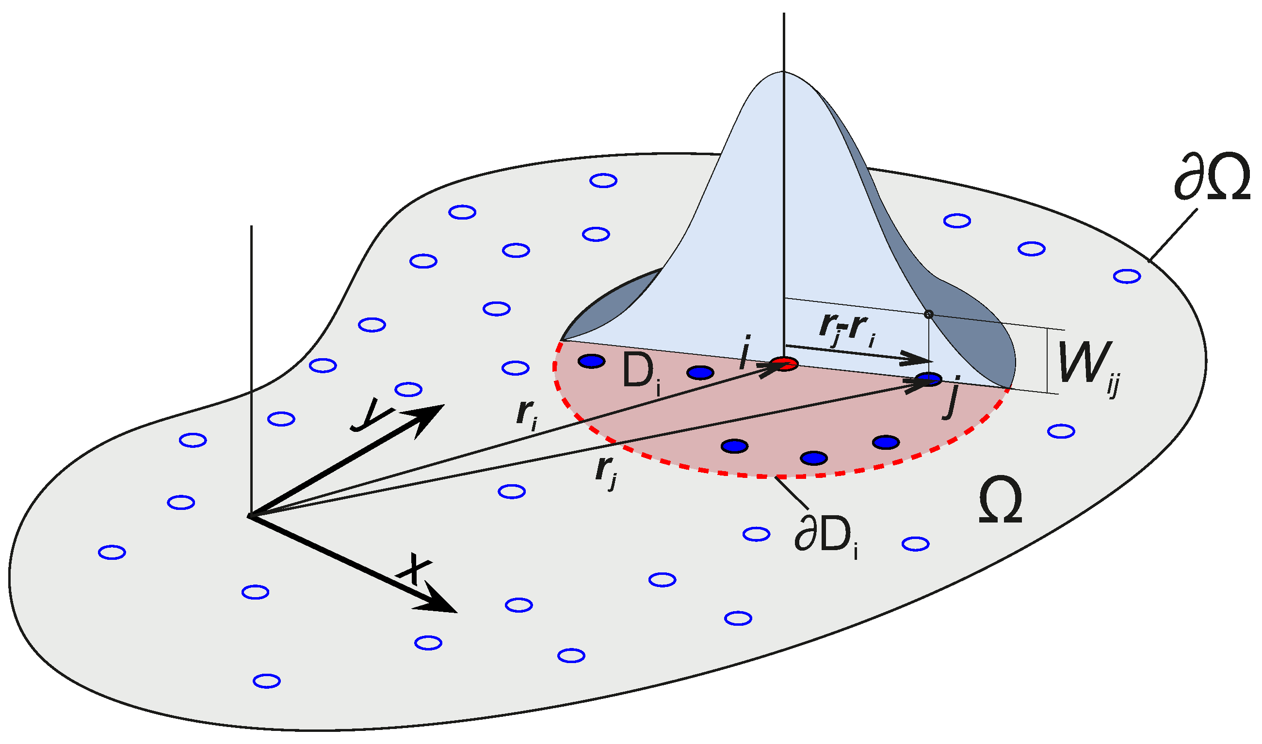
The computational domain $\mathsf{\Omega }$ is discretized by a set of N particles at positions ${\mathit{r}}_i={(x_i,y_i)}^T$. Index i is used to label particles and ranges from 1 to N. Each particle has an effective volume $V_i$. Besides the volume, particles have other properties that we refer with a generic variable ${\varphi }_i$. Moreover, each particle i has $n_i$ neighboring particles inside its compact support domain $D_i$ as schematically represented in Figure 1.

The SPH-ALE formulation was introduced by Vila and Ben Moussa [14,15] to increase the accuracy and stability of SPH methods in nonlinear systems of conservation laws. Vila and Ben Moussa applied this formulation to the Euler equations and presented a system of equations in semidiscrete form that has many similarities with the finite volume formalism. Since then, several developments were made by incorporating consolidated techniques used in mesh based methods like approximate and partial Riemann solvers, MUSCL, MOOD, and WENO [19,22,28].

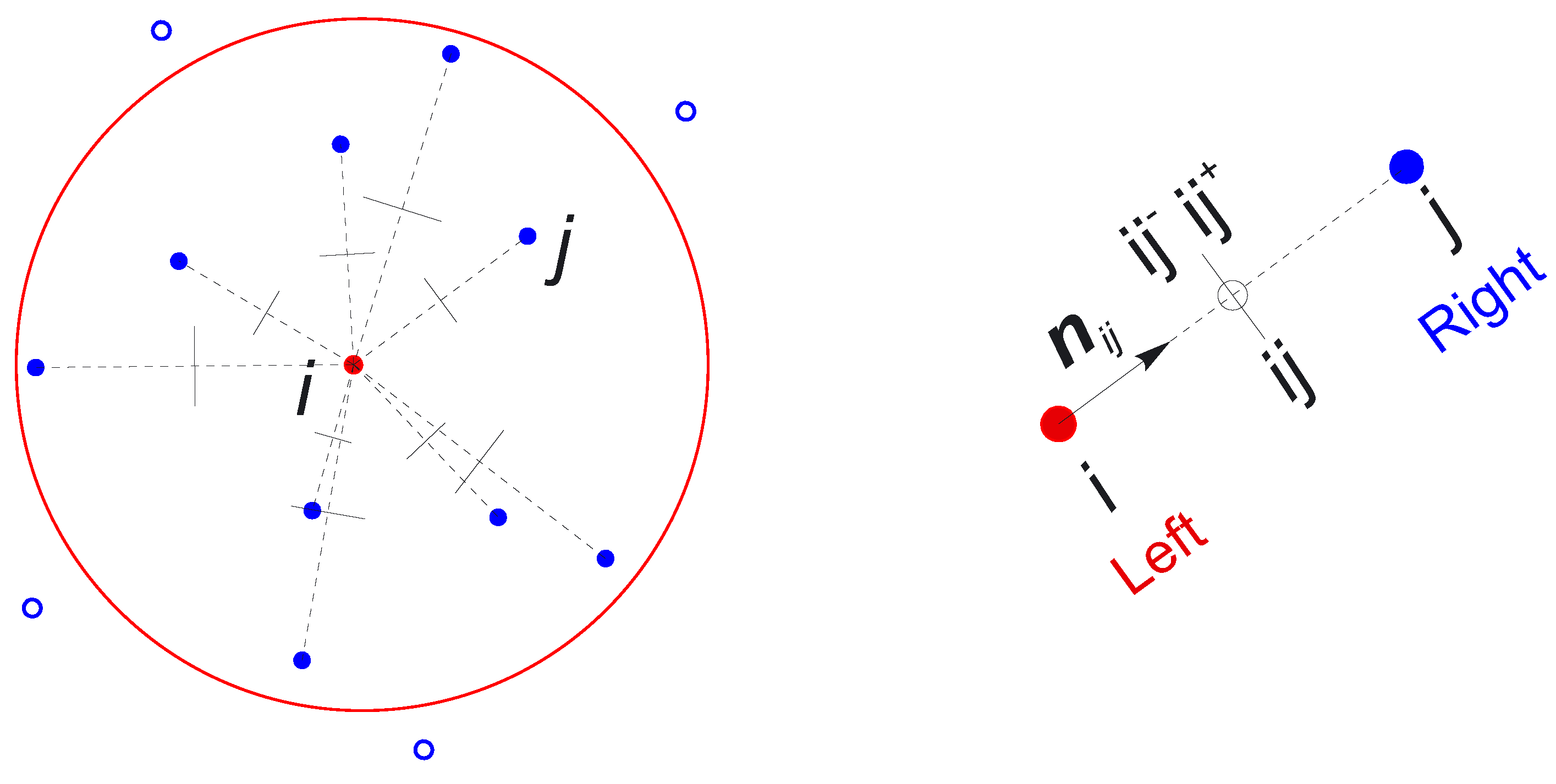
In the SPH-ALE formulation, the interaction of each neighboring particle j with the particle i admits a representation as a flux at the midpoint $ij$ located at ${\mathit{r}}_{ij}=\frac{1}{2}({\mathit{r}}_i+{\mathit{r}}_j)$. Fluxes are computed from solutions to one-dimensional moving Riemann problems. Thus, we can associate the particle i as the left state, particle j as the right state and the moving interface with the midpoint $ij$. Figure 2 shows the definition of one of the moving Riemann problems. Unit vector ${\mathit{n}}_{ij}$ points from particle i to particle j. We use index $i{j}^{-}$ and $i{j}^{+}$ to denote reconstruction values at the interface from the left and from the right. The kernel gradient can be expressed in terms of the unit vector ${\mathit{n}}_{ij}$. Kernel functions which depend only on the distance between particles can be expressed as $W_{ij}=W({\mathit{r}}_i-{\mathit{r}}_j,h_{ij})=W\left(q_{ij}\right)$, where $q_{ij}=\frac{∥{\mathit{r}}_i-{\mathit{r}}_j∥}{h_{ij}}$.

The gradient of the kernel function is given by $\nabla W_{ij}=\left|\frac{\partial W}{\partial q_{ij}}\right|\frac{1}{h_{ij}}{\mathit{n}}_{ij}$ showing that ${\mathit{n}}_{ij}$ and $\nabla W_{ij}$ are vectors with the same direction.

Several authors have proposed the SPH-ALE formulation for the Navier–Stokes equations [23,24,25]. In these works, the viscous term was discretized using an approximation of the Laplacian based on a hybrid SPH gradient by means of a first-order finite difference scheme [29]. In this work, we propose a different discretization for the viscous term of the Navier–Stokes equations. Observation of the Navier–Stokes in ALE form Equations (1)–(4) suggests that the viscous terms can be computed in the form of a diffusive flux, following a similar approach as the one used for the convective terms.

Thus, the proposed resulting semi-discretized form of the Navier–Stokes equations is given by

$$\begin{array}{cc}\hfill \frac{d\left(V_i{\mathit{U}}_i\right)}{dt}& {\displaystyle =-\sum _{j=1}^{n_i}{V}_i{V}_{j}2\left({\mathit{G}}_{ij}-{\mathit{H}}_i\right)·\nabla W_{ij}}\hfill \\ \hfill & {\displaystyle +\sum _{j=1}^{n_i}{V}_i{V}_{j}2\left({\mathit{F}}_{ij}^v-{\mathit{F}}_i^v\right)·\nabla W_{ij}+{\mathit{S}}_T{V}_i}\hfill \end{array}$$

(5)

$${\displaystyle \frac{d{V}_i}{dt}=\sum _{j=1}^{n_i}{V}_i{V}_{j}2\left({\mathit{w}}_{ij}-{\mathit{w}}_i\right)·\nabla W_{ij}}$$

(6)

where Equation (5) expresses the evolution of the conservative variables and Equation (6) describes the evolution of the effective volume associated to particle i. In the above equations, $W_{ij}=W({\mathit{r}}_i-{\mathit{r}}_j,h_{ij})$ is a kernel function and $h_{ij}=\frac{1}{2}(h_i+h_j)$ is the smoothing length. The length $h_i$ is linked to the particle volume via equation $h_i=\beta {V_i}^{\frac{1}{D}}$, where $\beta$ is a constant and D is the dimension of the computational domain. Throughout this work, we have set $\beta =2$. Note that, as the interparticle distance $dx$ can be estimated as $dx=V_i^{\frac{1}{D}}$, we adopt the practical consideration of linking the smoothing kernel length by a constant factor $\beta$ to the interparticle distance $dx$.

Moreover, we choose the cubic spline kernel proposed by Monaghan and Lattanzio [30] as kernel function. The support radius for cubic spline kernel is given by $R=2h_i=2\beta V_i^{\frac{1}{D}}=4V_i^{\frac{1}{D}}$. This implies that, for an initial uniform distribution of particles, $R=4dx$, resulting in 9 neighbors for 1D tests and 49 neighbors for 2D problems.

Tensors ${\mathit{G}}_{ij}$ and ${\mathit{F}}_{ij}^v$ in Equation (5) account for the Euler and viscous fluxes in the interface $ij$, respectively. The terms appearing with minus sign inside the parenthesis (${\mathit{H}}_i$ and ${\mathit{F}}_i^v$) are tensors evaluated at the position of particle i that assure at least zero order consistency at discrete level [19].

3.1. Discretization of the Convective Terms

The numerical flux tensor ${\mathit{G}}_{ij}$ is computed using the Rusanov flux in the co-moving frame according to

$${\mathit{G}}_{ij}=\frac{1}{2}({\mathit{H}}_{ij}^{+}+{\mathit{H}}_{ij}^{-})-\frac{1}{2}{S}_{ij}^{+}\mathsf{\Delta }{\mathit{U}}_{ij}·{\mathit{n}}^T$$

where ${\mathit{H}}_{ij}^{-}=\mathit{H}({\mathit{U}}_{ij}^{-},{\mathit{w}}_{ij})$ and ${\mathit{H}}_{ij}^{+}=\mathit{H}({\mathit{U}}_{ij}^{+},{\mathit{w}}_{ij})$ denote the approximations of the Lagrangian flux tensor $\mathit{H}=\mathbf{𝓕}\left(\mathit{U}\right)-\mathit{w}\otimes \mathit{U}$ on the left and right sides of the interface $ij$.

The term $S_{ij}^{+}$ is the maximum eigenvalue of the Jacobian matrix which in the Arbitrarian Lagrangian–Eulerian (ALE) framework reads

$$S_{ij}^{+}=max(({\mathit{u}}_{ij}^{+}-{\mathit{w}}_{ij})·{\mathit{n}}_{ij}+c_{ij}^{+},({\mathit{u}}_{ij}^{-}-{\mathit{w}}_{ij})·{\mathit{n}}_{ij}-c_{ij}^{-})$$

where $\mathsf{\Delta }{\mathit{U}}_{ij}={\mathit{U}}_{ij}^{+}-{\mathit{U}}_{ij}^{-}$ is the jump of the reconstructed conservative variables. Moreover, the term ${\mathit{w}}_{ij}$ is the velocity of the reference frame at the interface $ij$. On an Eulerian frame, ${\mathit{w}}_{ij}=0$, whereas on a Lagrangian frame ${\mathit{w}}_{ij}={\mathit{u}}_{ij}=({\mathit{u}}_{ij}^{+}+{\mathit{u}}_{ij}^{-})/2$.

We note that, despite the known diffusive behavior [31] of the Rusanov flux, it can be easily used with different EOS, so it is a convenient choice for the problems addressed here.

Tensor ${\mathit{H}}_i=\mathit{H}({\mathit{U}}_i,{\mathit{w}}_i)$ is the Lagrangian flux computed as a function of the state of the i-th particle ${\mathit{H}}_i=\mathbf{𝓕}\left({\mathit{U}}_i\right)-{\mathit{w}}_i\otimes {\mathit{U}}_i$.

In the SPH-ALE formulation, each particle i is associated with a velocity frame ${\mathit{w}}_i$ and a material velocity ${\mathit{u}}_i$. The velocity frame ${\mathit{w}}_i$ can be freely chosen and determines the evolution of particle positions. For the Eulerian approach of the method we set ${\mathit{w}}_i=0$ and particles are fixed in space. For the Lagrangian version, we set ${\mathit{w}}_i={\mathit{u}}_i$ and perform a weighted average interpolation of the velocity [32] to update particle positions. Therefore, the evolution of the particle position must satisfy for Eulerian/Lagrangian frame Equation (7).

$${\displaystyle \frac{d{\mathit{r}}_i}{dt}=0or\frac{d{\mathit{r}}_i}{dt}=\frac{{\displaystyle \sum _{j=1}^{n_i}{V}_j{\mathit{w}}_j{W}_{ij}}}{{\displaystyle \sum _{j=1}^{n_i}{V}_j{W}_{ij}}}}$$

(7)

3.2. High-Order Reconstruction and Moving Least Squares Approximations

One way to increase the accuracy of the resulting scheme is to compute the reconstruction of the variables at each integration point $ij$ using a high-order approximation. For a given variable $\varphi$, which is known on each particle, we can compute the reconstructed variable at integration point, ${\varphi }_{ij}$, by means of Taylor series as

$${\varphi }_{ij}^{+}={\varphi }_i+\nabla {\varphi }_i·\left({\mathit{r}}_{ij}-{\mathit{r}}_i\right)+\frac{1}{2}{\left({\mathit{r}}_{ij}-{\mathit{r}}_i\right)}^T{\nabla }^2{\varphi }_i\left({\mathit{r}}_{ij}-{\mathit{r}}_i\right),$$

(8)

where the first and successive derivatives are computed, following our previous work [22], using MLS approximations.

3.3. Viscous Terms Discretization

In this work, we propose to extend the same discretization that is typically performed in the Finite Volume method to SPH-ALE discretizations. Tensor ${\mathit{F}}_i^v={\mathit{F}}^v({\mathit{U}}_i,\nabla {\widehat{\mathit{U}}}_{\mathit{i}})$ is the viscous tensor computed as a function of the state of the i-th particle and the gradients obtained at integration point $ij$ as

$${\mathit{F}}_{ij}^v=\frac{1}{2}\left({\mathit{F}}_i^v+{\mathit{F}}_j^v\right)$$

(9)

where the derivatives required to evaluate the viscous tensor are computed with MLS reconstruction. Note that since the MLS reconstruction is performed for the convective terms, it does not require any additional reconstruction procedure to obtain a highly accurate discretization of the fluxes.

4. The Multi-Dimensional Optimal Order Detection (MOOD) Method

The a posteriori MOOD paradigm, introduced by Clain et al. [21], is used in this work to determine the optimal order of the polynomial reconstruction iteratively by building a candidate solution ${\mathbf{U}}^{*}$ for time $t^{n+1}$ based on the $t^n$ solution. The candidate solution is then run by a series of detectors that check if the solution has a certain set of desirable properties. If any of the particles is flagged as invalid, the candidate solution at that particle is discarded and recomputed from the original solution at $t^n$ but using a more dissipative scheme by lowering the polynomial reconstruction degree.

4.1. Mood Loop

The MOOD approach is composed of a Particle Polynomial Degree (PPD) and a chain of detectors. The PPD refers to the actual polynomial degree used to compute the candidate solution ${\mathbf{U}}^{*}$. We evaluate the flux at the midpoint $ij$ between particles i and j, taking the minimum of the respective PPDs for the polynomial reconstruction as $\mathrm{P}\mathrm{P}{\mathrm{D}}_{ij}=min\left(\mathrm{PPD}\left(i\right),\mathrm{PPD}\left(j\right)\right)$. The chain of detectors controls the validity of the resulting solution and the particle’s PPD is decremented where any of the detectors flag the solution as invalid.

The MOOD loop iterates through the PPD map, initialized with maximal order $d_{max}=3$, decreasing the order of the particles that present a non-physical or invalid solution. In this work only orders 3 and 1 are used, being the order 1 called the parachute scheme that, by definition, fulfills all the detectors requirements.

If the PPD map is modified, the candidate solution is declared not valid and therefore must be recomputed. Note that only the particles where the PPD map is modified are recomputed.

4.2. Chain Detectors

In order to obtain a stable solution within the SPH formulation, a chain of detectors is used to assess whether the solution is admissible or not. In this work, we employ two detectors:

• Physical Admissibility Detector (PAD): it checks that all the particles in the solution have positive density and pressure at all times. It also accounts for NaN (Not a Number) values that arise in the candidate solution.
• Numerical Admissible Detector (NAD) [33]: relaxed version of the Discrete Maximum Principle (DMP) [21]. It checks that the solution is monotonic and thus, no new extrema are created. It compares the candidate solution with the solution obtained in the previous Runge–Kutta step.

$$\underset{\mathbf{y}\in {\mathcal{V}}_i}{min}\left({\mathbf{U}}^{\mathrm{RK}}\left(\mathbf{y}\right)\right)-\delta ⩽{\mathbf{U}}^{*}\left(\mathbf{x}\right)⩽\underset{\mathbf{y}\in {\mathcal{V}}_i}{max}\left({\mathbf{U}}^{\mathrm{RK}}\left(\mathbf{y}\right)\right)+\delta$$

(10)

where ${\mathcal{V}}_i$ is the set of closest particles and the tolerance $\delta$ is defined following [33] as

$$\delta =max\left({10}^{-4},{10}^{-3}·\left(\underset{\mathbf{y}\in {\mathcal{V}}_i}{max}\left({\mathbf{U}}^{\mathrm{RK}}\left(\mathbf{y}\right)\right)-\underset{\mathbf{y}\in {\mathcal{V}}_i}{min}\left({\mathbf{U}}^{\mathrm{RK}}\left(\mathbf{y}\right)\right)\right)\right)$$

(11)

5. Numerical Tests

We present the numerical tests selected to assess the ability of the SPH-ALE-MOOD scheme to produce accurate and robust approximations. All the numerical examples have been computed using a third-order Runge–Kutta scheme for time integration.

5.1. 1d Riemann Problems

The first test cases are devoted to assess the stability and diffusive properties of the SPH-ALE-MOOD scheme. Here, we consider several one-dimensional tests.

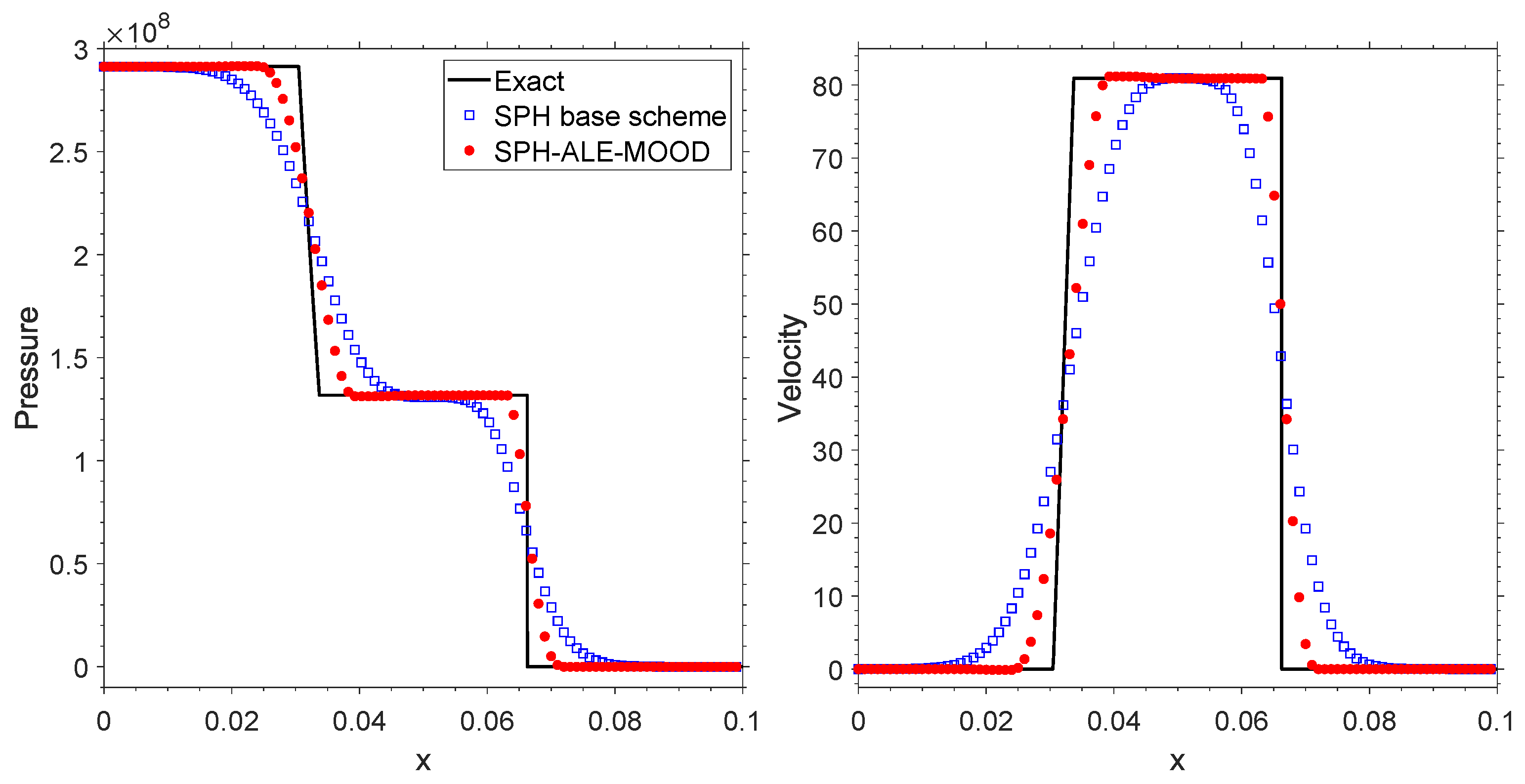
The first test case is the 1D Riemann problem (R1) which is one of the four proposed by Marongiu in [34]. In the context of SPH, the works presented in [11,18] also simulate this 1D Riemann problems with Tait EOS. The fluid is water modeled with Tait EOS (${\rho }_0=1000$ kg/m³, $c_0=1466.0$ m/s, $\gamma =7$ and $p_0=0$ Pa). The domain is $[0,0.1]$ m and the initial condition is defined as

$$\left(\mathrm{R}1\right)(\rho ,u)=\left\{\begin{array}{cc}(1100{\mathrm{kg}/\mathrm{m}}^3,0\mathrm{m}/\mathrm{s}),\hfill & \hfill \mathrm{if}x\le 0.05\mathrm{m}\\ (1000{\mathrm{kg}/\mathrm{m}}^3,0\mathrm{m}/\mathrm{s}),\hfill & \hfill \mathrm{otherwise}\end{array}\right.$$

A discretization of 100 particles is used and the solution is advanced up to $t_{final}={10}^{-5}$ s. The exact solution consists of a rarefaction wave traveling to the left and a shock wave traveling to the right. As a reference solution, we use the exact solution obtained with the algorithm given in [35] applied to the Tait EOS as indicated in [36].

Figure 3 plots the pressure and velocity profiles obtained with the base scheme (first-order SPH-ALE scheme) [15] and with the SPH-ALE-MOOD model. The SPH-ALE base scheme smears the solution in the shock and rarefaction wave. As expected, for the same number of particles the SPH-ALE-MOOD provides a better representation of the shock front. The front and tail of the rarefaction wave provided for the SPH-ALE-MOOD are also accurately captured and are free of overshoots near discontinuities. Both Eulerian and Lagrangian versions of the scheme produce very similar results, so we only plot here the results obtained with the Lagrangian description.

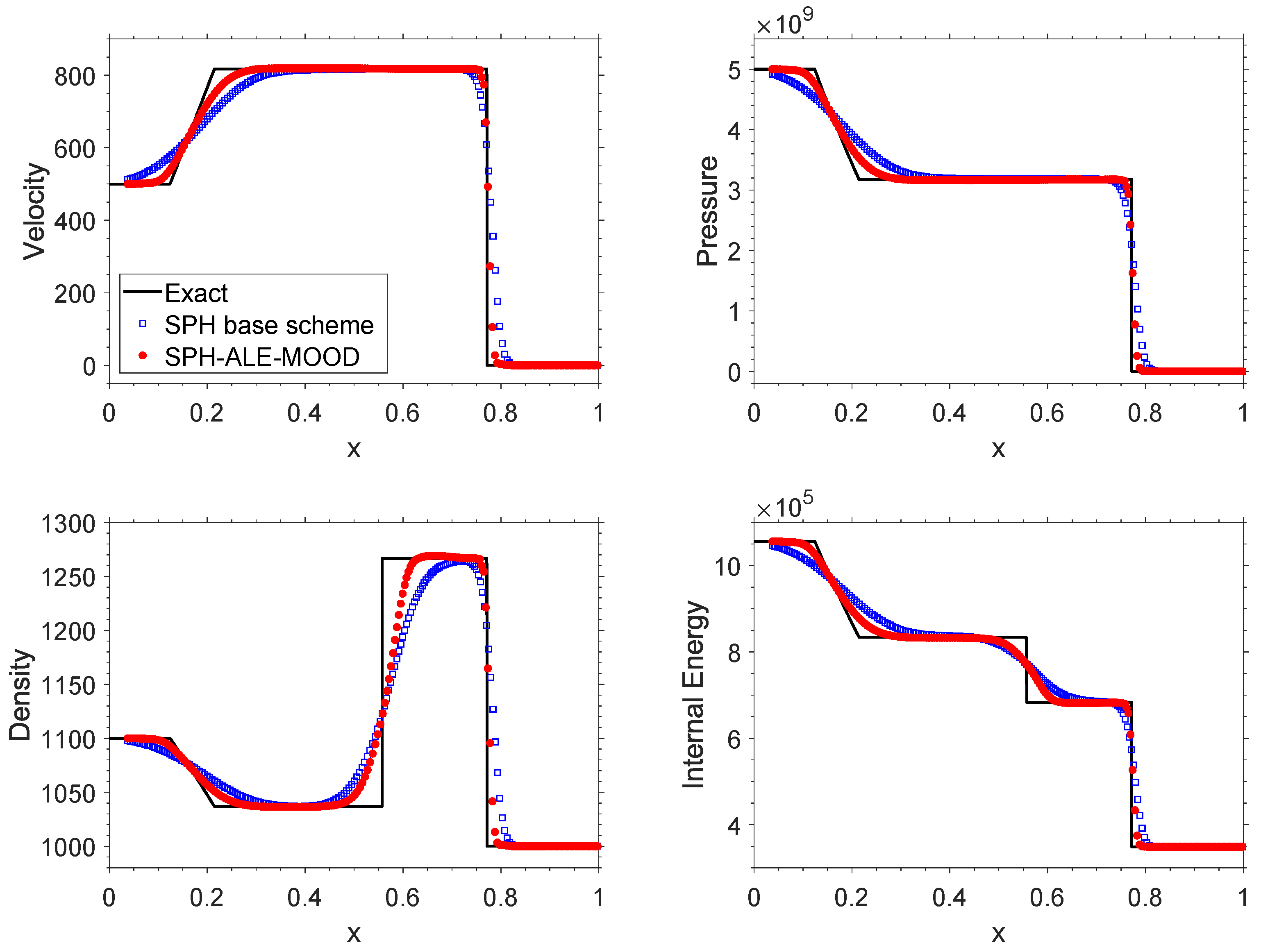
We consider a second one-dimensional Riemann problem (R2). In this case, the liquid is assumed to follow the Tamman EOS ($\gamma =7.15$ and $p_c=3\times {10}^8$ Pa). This test was proposed by Ivings and Toro in [36] and has been also presented in [37] with a SPH-ALE code with MUSCL reconstruction using a minmod limiter and a finer particle resolution. The initial conditions for this problem are

$$\left(\mathrm{R}2\right)(\rho ,u,p)=\left\{\begin{array}{cc}(1100{\mathrm{kg}/\mathrm{m}}^3,500\mathrm{m}/\mathrm{s},5\times {10}^9\mathrm{Pa}),\hfill & \hfill \mathrm{if}x\le 0.5\mathrm{m}\\ (1000{\mathrm{kg}/\mathrm{m}}^3,0,1\times {10}^5\mathrm{Pa}),\hfill & \hfill \mathrm{otherwise}\end{array}\right.$$

The exact solution to this problem comprises a left-going rarefaction wave, a contact discontinuity and a right-going shock wave. The computational domain $[0,1]$ is discretized with 200 particles.

In Figure 4 we plot the results for pressure, velocity, density, and internal energy at the final time $t_{final}=7\times {10}^{-5}$ s obtained with the SPH base scheme and the SPH-ALE-MOOD using a Lagrangian description. The SPH-ALE-MOOD improves the results of the SPH base scheme in all the salient features present in the flow. In the density and internal energy plots, it is observed that the resolution of the contact discontinuity is not as sharp as the one obtained for the shock front. We note that the smearing in the contact discontinuity is inherent to the approximations made in the derivation of the Rusanov flux as reported in previous works [19,22].

5.2. 2d Blast Explosion

The first two-dimensional test considered here is an extension of the one-dimensional shock tube R1 assuming cylindrical symmetry. The fluid is water modeled with Tait EOS (${\rho }_0=1000{\mathrm{kg}/\mathrm{m}}^3$, $c_0=1466.0\mathrm{m}/\mathrm{s}$, $\gamma =7$ and $p_0=0\mathrm{Pa}$). The computational domain is a circle of radius $R=0.1\mathrm{m}$ centered at the origin and the initial conditions are given by

$$(\rho ,u,v)=\left\{\begin{array}{cc}(1100{\mathrm{kg}/\mathrm{m}}^3,0\mathrm{m}/\mathrm{s},0\mathrm{m}/\mathrm{s}),\hfill & \hfill \mathrm{if}r\le 0.05\mathrm{m}\\ (1000{\mathrm{kg}/\mathrm{m}}^3,0\mathrm{m}/\mathrm{s},0\mathrm{m}/\mathrm{s}),\hfill & \hfill \mathrm{otherwise}\end{array}\right.$$

The configuration mimics an explosion with a shockwave traveling outwards and a rarefaction moving towards the origin. The reference solution is obtained by using a one dimensional finite volume code with a very fine mesh as explained in [35].

The evolution of the flow is simulated until $t_{final}={10}^{-5}$ s with the SPH-ALE-MOOD scheme.

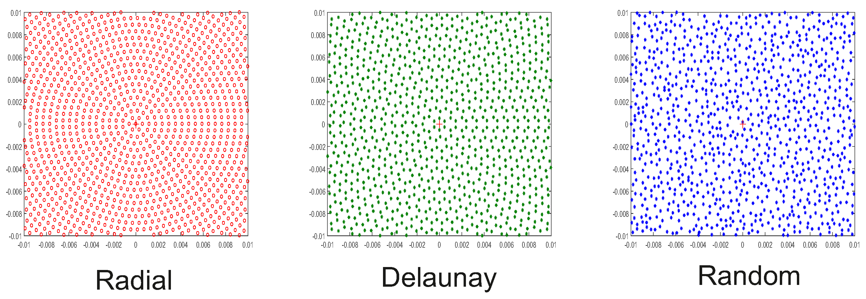
We consider three different particle initializations to evaluate the effects of the initial positions of the particles on the quality of the numerical results. A radial distribution disposing particles in rings, a Delaunay distribution, which places particles in barycenters of triangles and finally, the third initial layout of particles is the result of applying a random displacement to the Delaunay distribution. The number of particles of the radial distribution (∼90,000) is slightly higher than the one of the Delaunay and Random distribution (∼75,000). Figure 5 shows the initial distributions considered.

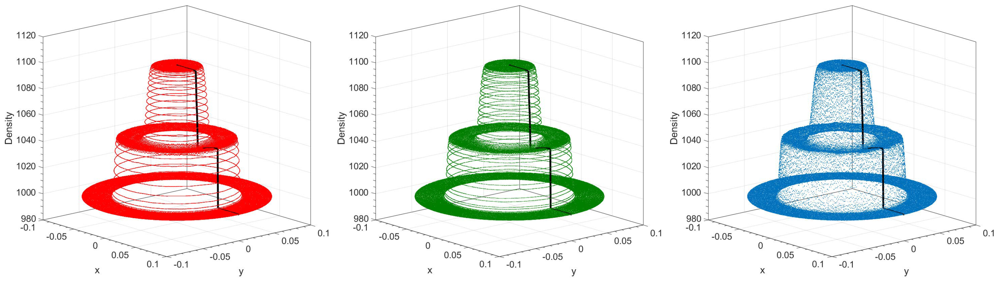
Figure 6 shows the density at final time for the three initial particle layouts. The reference solution is represented with a black solid line. It is observed that the results preserve the radial symmetry of the physical problem.

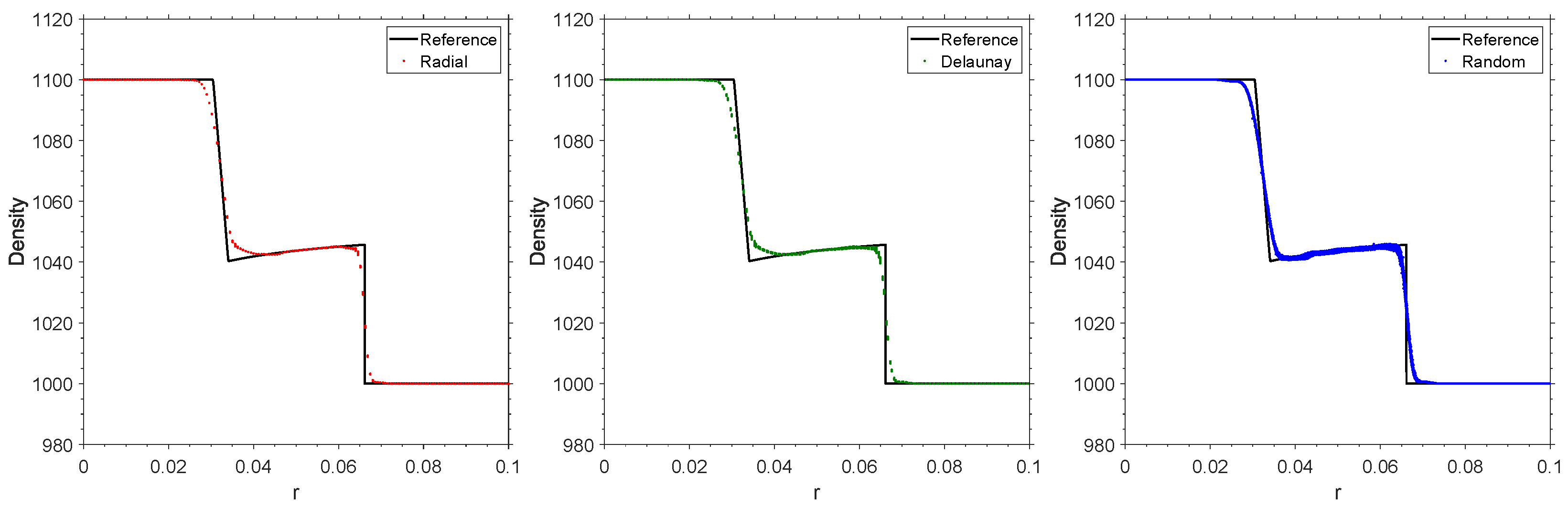
Figure 7 plots the density profiles along the radial coordinate. All the particles of the computational domain are represented and it can be noticed more clearly the ability of the model to preserve the radial symmetry. We note that the dispersion of the particles is really small for all particle distributions.

5.3. Taylor–Green Flow

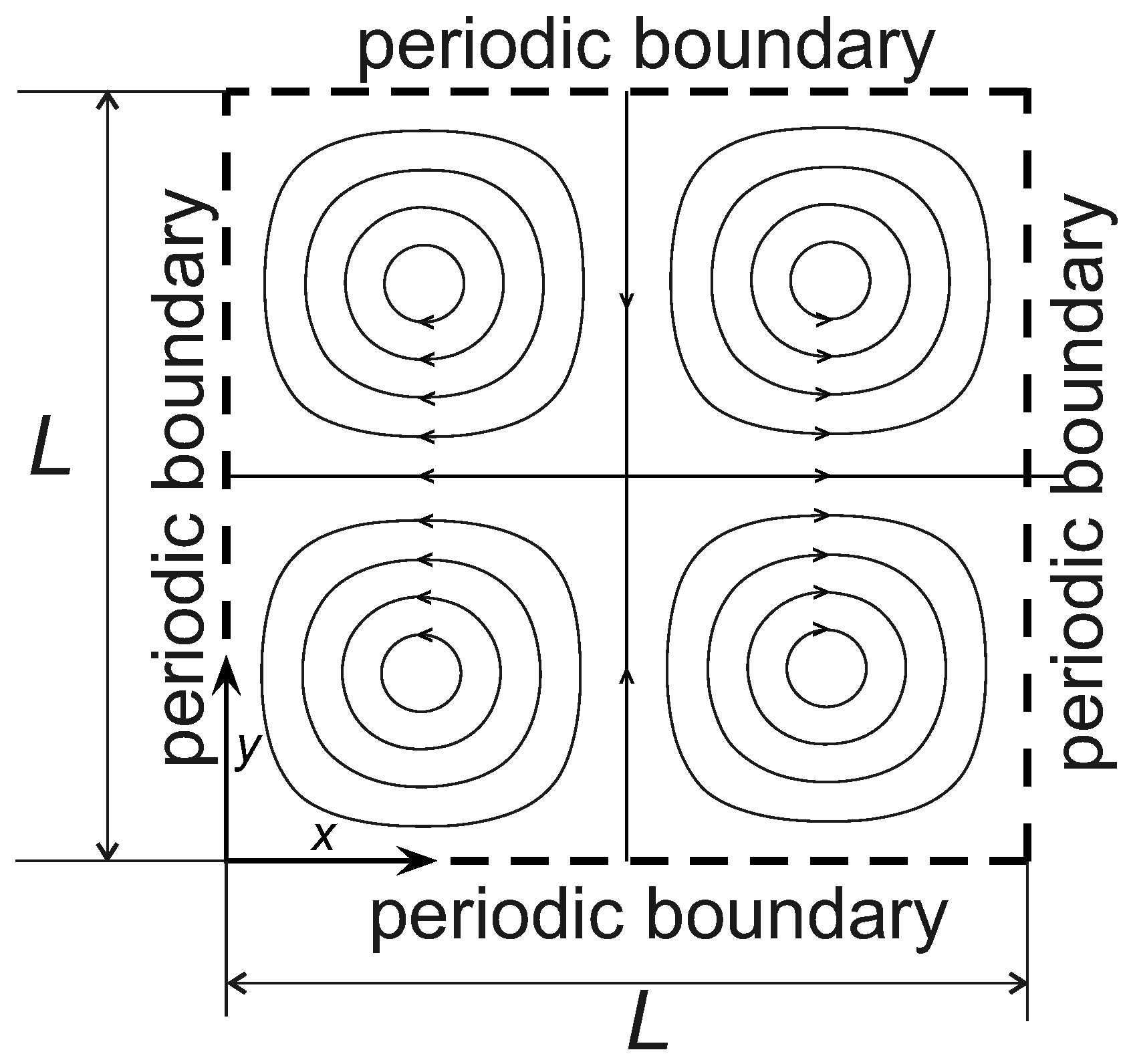
The Taylor–Green flow is a classical test for numerical methods for the simulation of viscous flows. It provides an exact solution of the incompressible Navier–Stokes equations in a periodic domain [38,39]. The flow involves the decay of four counter-rotating vortices within the periodic region of size $L\times L$ as shown in Figure 8

The exact solution is given in [40] and reads

$${\displaystyle \frac{u}{U_0}}=sin\left(\frac{2\pi x}{L}\right)cos\left(\frac{2\pi y}{L}\right)exp\left(-\frac{8{\pi }^2}{Re}\frac{U_0}{L}t\right)$$

(12)

$${\displaystyle \frac{v}{U_0}}=-cos\left(\frac{2\pi x}{L}\right)sin\left(\frac{2\pi y}{L}\right)exp\left(-\frac{8{\pi }^2}{Re}\frac{U_0}{L}t\right)$$

(13)

$${\displaystyle \frac{p}{\frac{1}{2}{\rho }_0{U}_0^2}}={\displaystyle \frac{1}{2}}\left[cos\left(\frac{4\pi x}{L}\right)+cos\left(\frac{4\pi y}{L}\right)\right]exp\left(-\frac{16{\pi }^2}{Re}\frac{U_0}{L}t\right)$$

(14)

where $Re$ is the Reynolds number of the flow, defined as $Re=\frac{{\rho }_0{U}_{0}L}{{\mu }_0}$. $U_0$ is a reference velocity magnitude, and ${\rho }_0$ and $\mu$ are constant values for the density and viscosity of the fluid, respectively.

A global decay kinetic energy factor, denoted by $r\left(t\right)$, is defined as the ratio of the overall kinetic energy at time t ($E_k$) and the corresponding one to initial time $E_{k0}$

$$r\left(t\right)=\frac{E_k}{E_{k0}}=\frac{{\int \int }_D\frac{1}{2}[u^2(x,y,t)+v^2(x,y,t)]dxdy}{{\int \int }_D\frac{1}{2}[u^2(x,y,0)+v^2(x,y,0)]dxdy}$$

(15)

Evaluation of (15) with the velocity field given by Equations (12) and (13) results in an exponential decay according to

$$r\left(t\right)=\frac{E_k}{E_{k0}}=exp\left(-\frac{16{\pi }^2}{Re}\frac{U_0}{L}t\right)$$

(16)

and by integration in the domain results $E_{k0}=\frac{1}{4}{U}_0^2{L}^2$.

For the simulations presented in this test, we consider a Taylor–Green flow with $L=1$ m, $U_0=1$ m/s and ${\rho }_0=$1 kg/m³. According to the weakly compressible approach, we assume that the fluid obeys the Tait equation with parameters ${\rho }_0=1$ kg/m³, $c_0=10$ m/s, $\gamma =7$ and $p_0=0$ Pa. The case is simulated for $Re=10$, $Re=100$ and $Re=1000$ with the Eulerian version of the SPH-ALE-MOOD scheme. Fluid particles are disposed inside the square domain on a Cartesian arrangement with $dx=dy=1/100$ as shown in Figure 9.

The initial conditions are computed using Equations (12)–(14) with the value of the density obtained from the Tait EOS for the analytical pressure.

Figure 10 shows the velocity components and pressure at non-dimensional time $t^{*}=t{U}_0/L=1$. Velocity and pressure are smooth, similar to the analytical solution and no degradation of the vortical pattern is observed.

Figure 11 shows the time evolution of global decay of the kinetic energy, $r\left(t\right)$, and the maximum velocity modulus obtained using the SPH-ALE-MOOD method and the corresponding reference incompressible solution for three different Reynolds numbers: $Re=10$, $Re=100$, and $Re=1000$. The numerical results are in close agreement with the analytical solution, showing that the high-order reconstruction of the proposed scheme allows achieving a low dissipation scheme which is accurate for a wide range of $Re$ numbers.

Following the work in [41], we have measured the time evolution of the pressure at the center of the domain for $Re=100$ and $Re=1000$ cases. The results are compared in Figure 12 with the theoretical solution and the solutions obtained with the $\delta$-SPH and ${\delta }^{+}$-SPH presented by Sun et al. [41,42]. We note that the proposed scheme shows better agreement with the reference solution for all particle resolutions. Moreover, it is remarkable the reduced amount of pressure oscillations, even for coarse discretizations.

In Figure 13, the pressure field along $y=0.5L$ is shown at $t^{*}=6$ for $Re=1000$. The results closely follows the theoretical solution even for the coarser discretization.

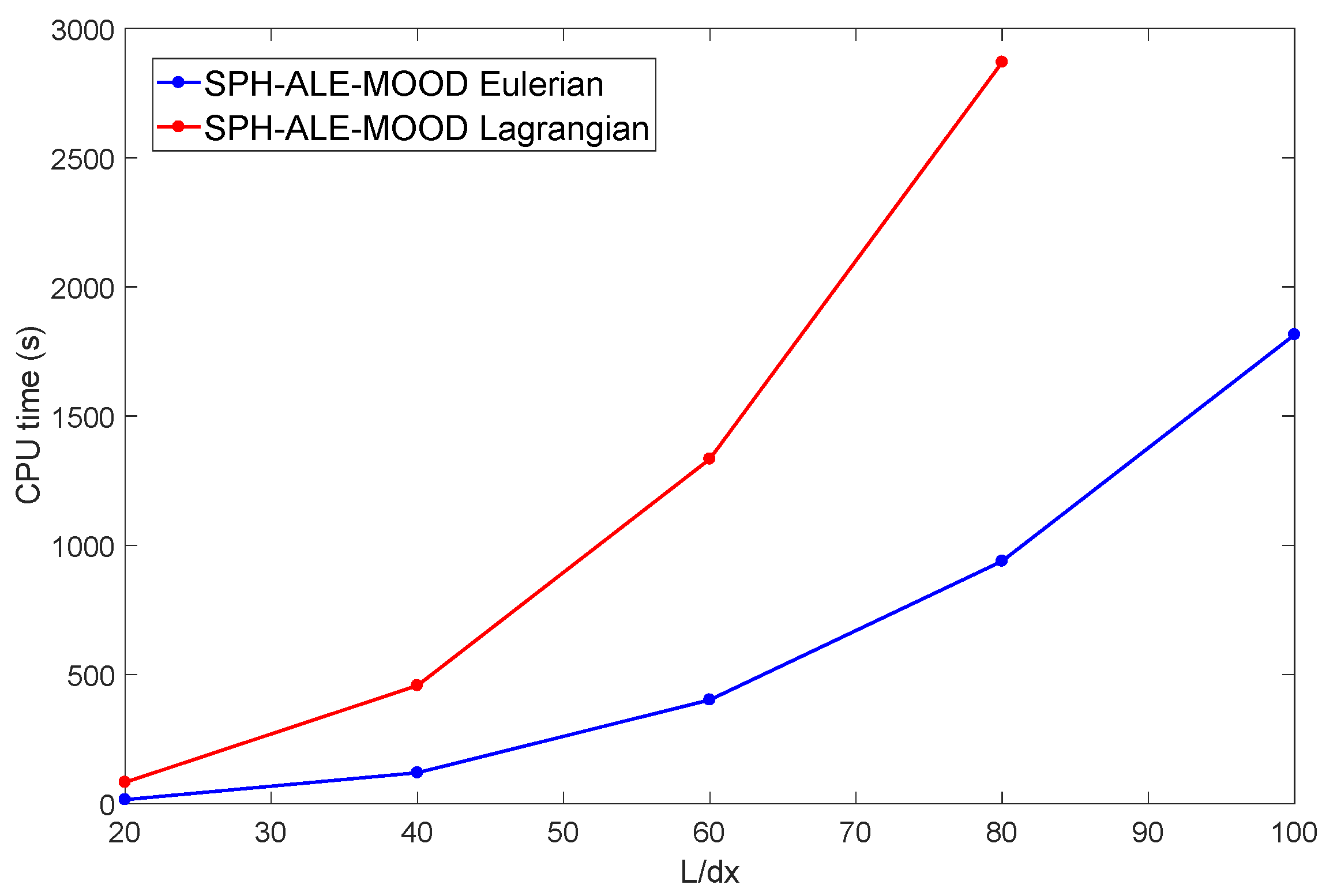
Concerning the computational cost of the proposed scheme, Figure 14 plots the CPU time consumed for different particle discretizations for a simulation until a final time of $t^{*}=2$ for $Re=100$. As expected, the Eulerian scheme is faster than the Lagrangian method. Then, a possible way for improving the efficiency of the proposed method is to combine Eulerian and Lagrangian particles. This idea has been explored previously in the context of ISPH [43] and fits very naturally in the proposed formulation.

5.4. Couette and Poiseuille Flows

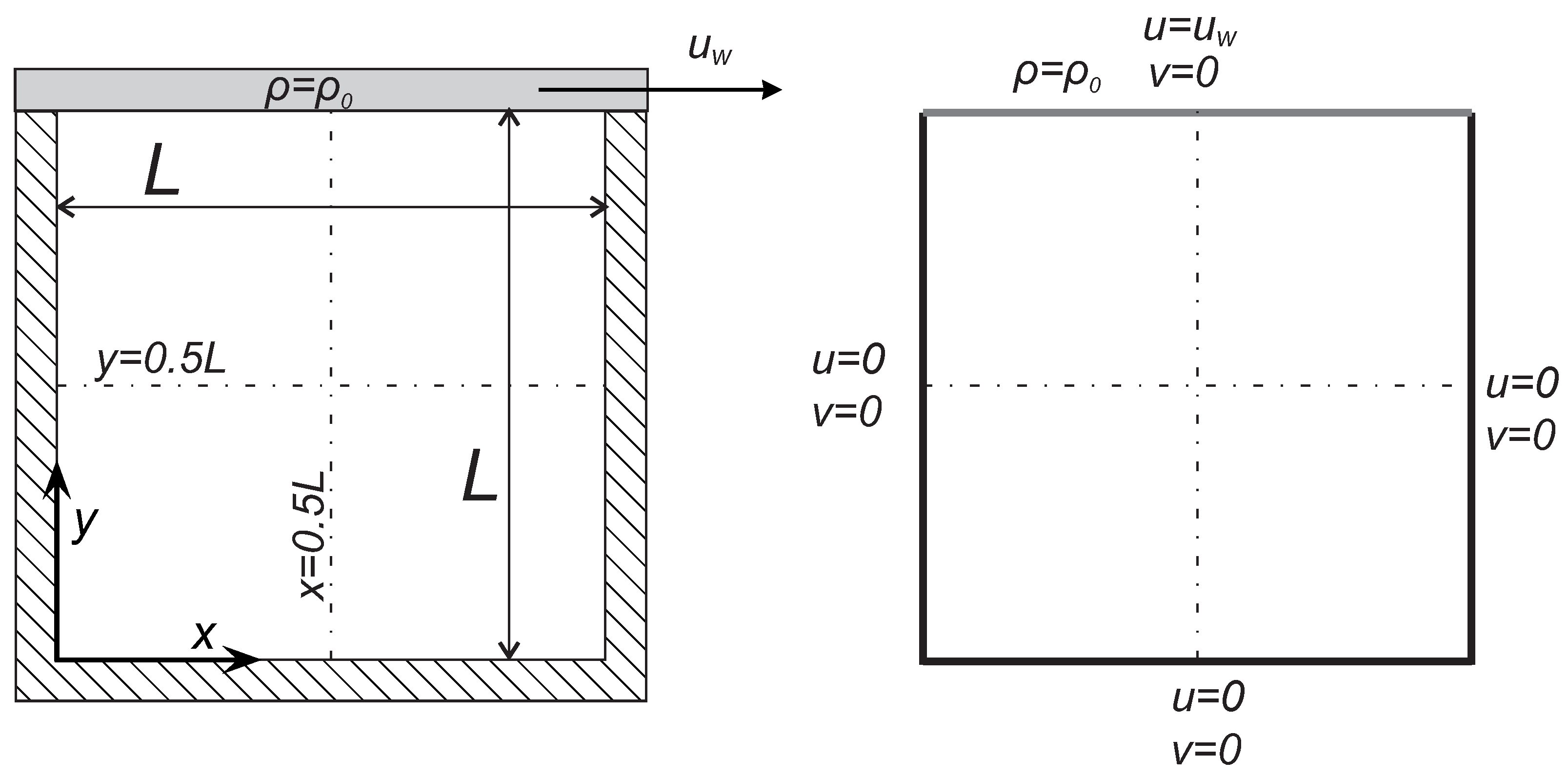
Couette and Poiseuille flows are special configurations of the incompressible Navier–Stokes equations that have analytical solution [44]. In both cases, a Newtonian fluid moves between two infinite parallel plates. The Couette flow is driven by the movement of one of the plates whereas the Poiseuille flow is driven by a pressure gradient. As velocity does not vary along the flow direction, a finite length of the plates is considered with periodic boundary condition in left and right sides. Figure 15 shows the geometry model and boundary conditions considered for the simulations. In both configurations the fluid is initially at rest.

In the Couette flow, the time-dependent exact solution for the fluid velocity in the x-direction can be expressed as [44,45]

$$u(y,t)=\frac{u_p}{L}y+\sum _{n=1}^{\infty }\frac{2u_p}{n\pi }{(-1)}^{n}sin\left(\frac{n\pi }{L}y\right)exp\left(-\nu \frac{n^2{\pi }^2}{L^2}t\right)$$

(17)

where $u_p$ is the horizontal velocity of the upper plate and $\nu$ is the kinematic viscosity of the fluid.

Similarly, for the Poiseuille flow the transient exact solution is given by [44,45]

$$u(y,t)=\frac{f_x}{2\nu }y(y-L)+\sum _{n=0}^{\infty }\frac{4f_x{L}^2}{\nu {\pi }^3{(2n+1)}^3}sin\left(\frac{\pi y}{L}(2n+1)\right)exp\left(-\frac{{(2n+1)}^2{\pi }^2\nu }{L^2}t\right)$$

(18)

where $f_x$ denotes a force source term in the x-momentum equation and, as such, it must be included in the source term ${\mathit{S}}_T$ of the system of equations defined in (4). The force source term $f_x$ and the steady peak velocity in the midplane of the channel $u_{peak}$ are related by expression $u_{peak}=\frac{1}{8\nu }{f}_x{L}^2$.

For both problems, the Reynolds number is defined as $Re=\frac{u_{max}L}{\nu }$ considering the distance between plates L and the maximum velocity $u_{max}$ as the reference length and velocity scales.

In this work, we conduct Couette and Poiseuille simulations for $Re=10$. The same value was adopted in the works of Chiron [23], Ferrand [46], and Fourtakas [47]. The fluid is modeled using the Tait equation with ${\rho }_0=1{\mathrm{kg}/\mathrm{m}}^3$, $\gamma =7$, $c_0=10\mathrm{m}/\mathrm{s}$, and $p_0=0\mathrm{Pa}$. The kinematic viscosity considered for the fluid is $\nu =0.1{\mathrm{m}}^2/\mathrm{s}$. The distance between plates is set to $L=1\mathrm{m}$ and half of this distance is considered for the periodic length in the flow direction.

In the Couette flow, $u_p$ is set to $1\mathrm{m}/\mathrm{s}$, which leads to $Re=10$. For the Poiseuille flow, we impose the force source term as $f_x=0.8{\mathrm{m}/\mathrm{s}}^2$ to produce the same $Re$ number.

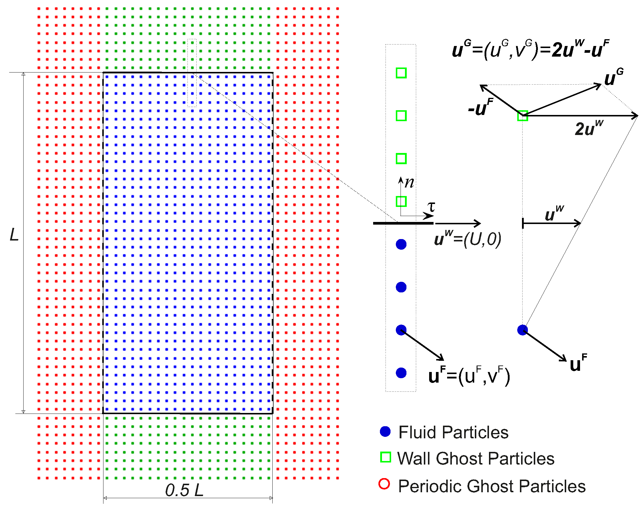
Figure 16 shows the arrangement of the particles employed for both the Couette and Poiseuille tests. The number of fluid particles between walls and periodic zones is 40 and 20, respectively, resulting in a squared arrangement with distance between particles $dx=L/40$.

In addition to the fluid particles, we need to incorporate ghost particles for implementing the periodic and wall boundary conditions. For the wall ghost particles we follow the technique used in [13]. A schematic representation of this technique is shown on the right of Figure 16. Dirichlet boundary conditions for velocity on the wall require that ghost particles update their velocity ${\mathit{u}}^G={(u^G,v^G)}^T$ following the vector equation.

$${\mathit{u}}^G=2{\mathit{u}}^W-{\mathit{u}}^F$$

(19)

where ${\mathit{u}}^F={(u^F,v^F)}^T$ is the velocity of the mirroring fluid particle and ${\mathit{u}}^W={(u^W,v^W)}^T$ is the velocity vector of the wall. In case of fixed walls ${\mathit{u}}^W={(0,0)}^T$ and for the top moving wall in Couette flow ${\mathit{u}}^W={(u_p,0)}^T$.

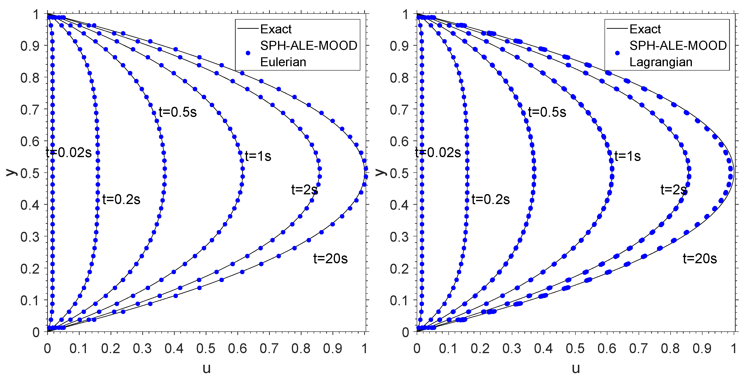
As we already have commented, one of the main advantages of the SPH-ALE method is the ability to use either Eulerian or Lagrangian description, and both configurations are able to obtain accurate solutions for this test case. Figure 17 shows the velocity profiles obtained with the SPH-ALE-MOOD scheme for Poiseuille flow at $Re=10$ for the Eulerian and Lagrangian description. The exact solution is computed using Equation (18). For $t=20$ s the flow is practically in the steady state condition and the obtained numerical solutions agree almost perfectly with the exact solution.

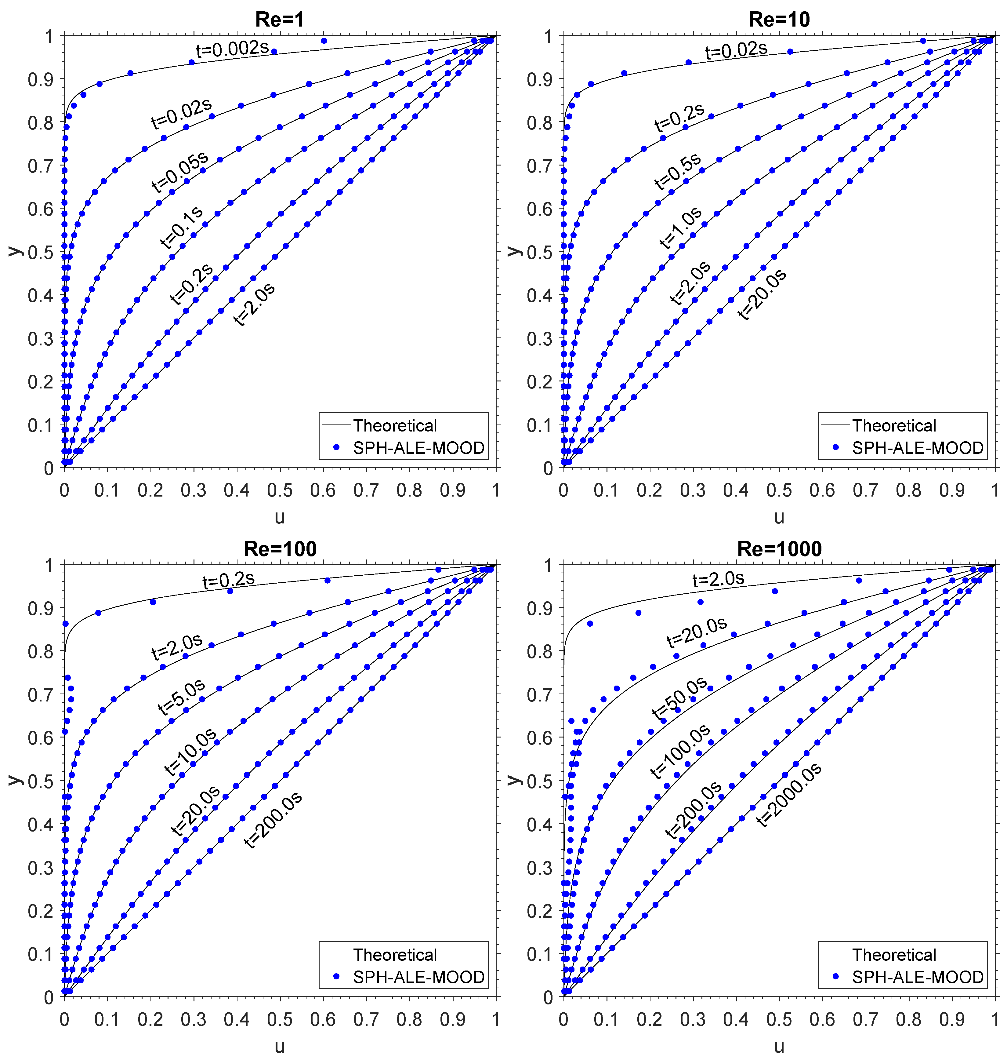
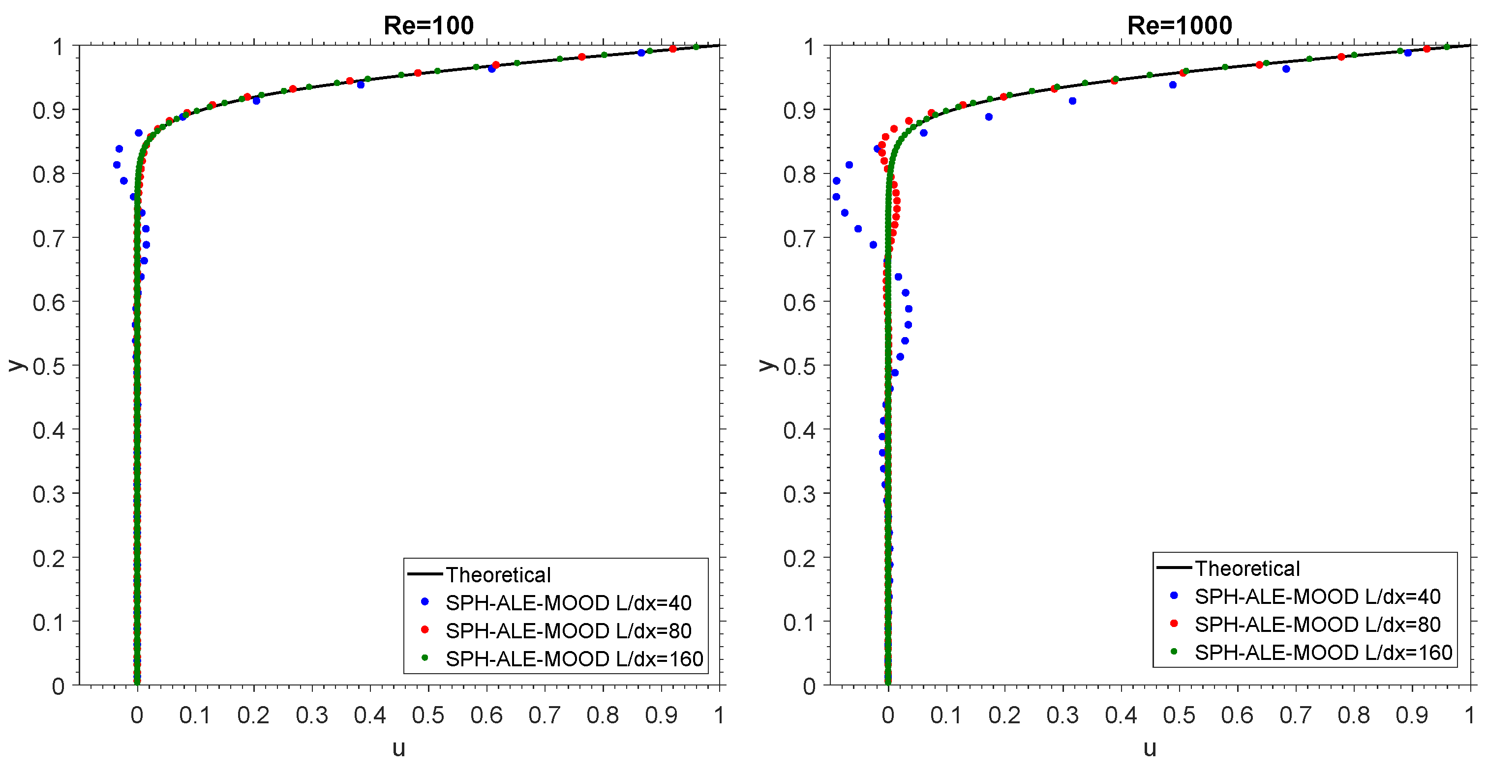
Figure 18 shows the velocity profiles obtained with the SPH-ALE-MOOD scheme for the Couette flow at $Re=1,10,100,1000$. The exact solution is computed using Equation (17). At $t=0$, the velocity of the moving plate changes abruptly from rest to an horizontal velocity $u_p$ forming a sharp discontinuity in the velocity field. A short time after that event, the obtained numerical results slightly deviates over the exact solution. This effect increases with the Reynolds number. For the last time instant, displayed for each Reynolds in Figure 18, the flow has practically reached the steady state, and the velocity profile is linear. The obtained results in the steady state are in close agreement with the exact solution for all the Reynolds numbers computed in this test case.

In Figure 18, the deviation from the reference solution observed in the first time instants of the simulations for $Re=100$ and $Re=1000$, are due to a lack of particles. For these Reynolds numbers, the spatial discretization is not able to capture the abrupt change in the velocity. To verify this, we plot in Figure 19 the results obtained for $Re=100$ at $t=0.2$ (left) and $Re=1000$ at $t=2$ (right) for different particle resolutions. It is seen that as the particle resolution increases the deviation is reduced, as expected.

5.5. 2d Lid-Driven Cavity Flow

The final test presented to assess the behavior of the proposed method is the 2D flow inside a square lid-driven cavity of length L. A schematic setup of the geometry is shown in Figure 20. The lateral and bottom walls are stationary, while the top wall moves horizontally to the right at speed $u_w$.

Different Reynolds numbers, namely, $Re=100$, $Re=400$, and $Re=1000$, are studied and results are compared to Ghia [48]. As in the previous case, the velocity of the frame is set to zero adopting the Eulerian version of the SPH-ALE-MOOD scheme.

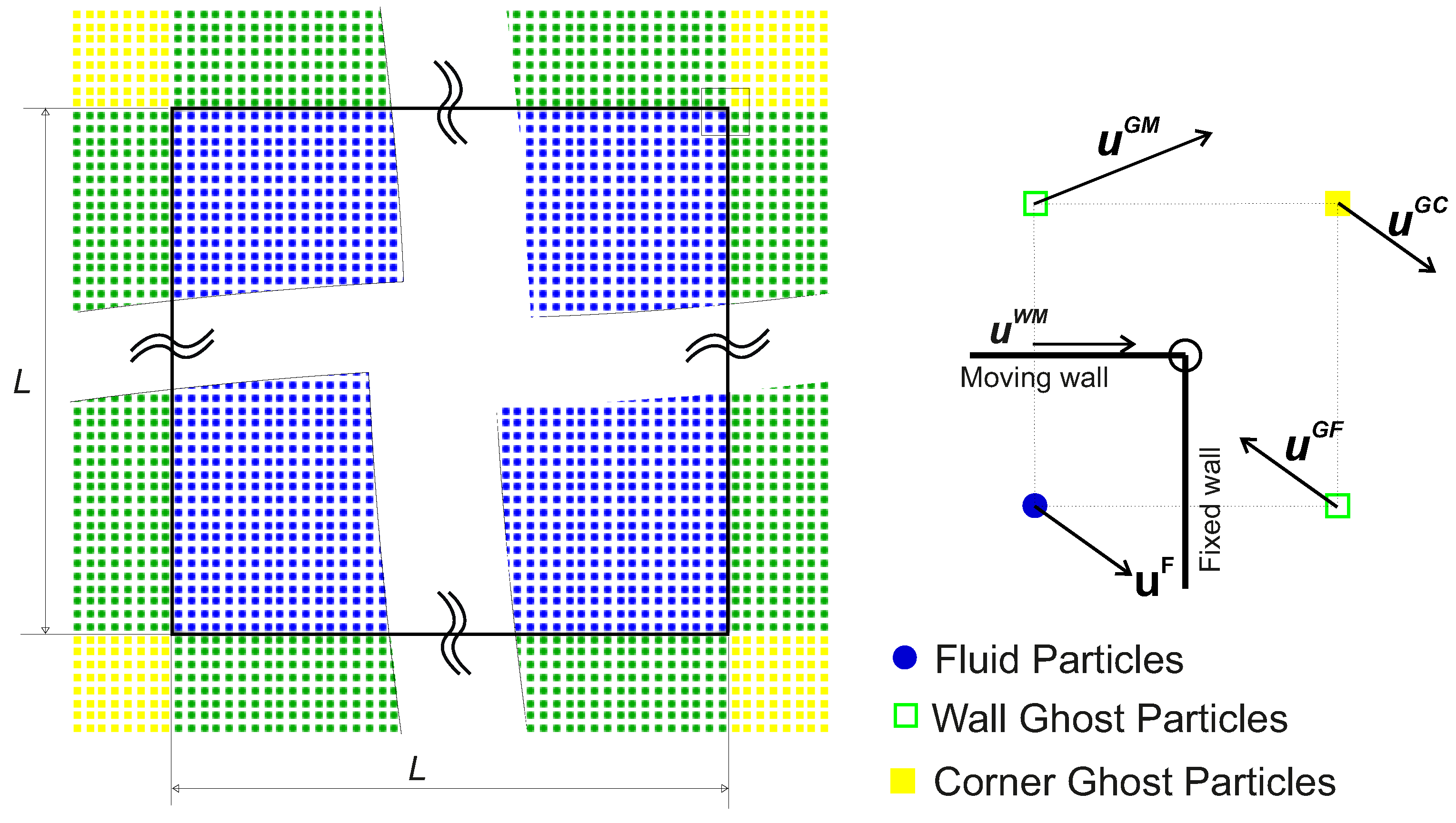
Figure 21 shows the layout and the type of particles. A Cartesian layout is adopted using a discretization of 100 particles on each side. Lid-driven cavity does not introduce any new type of boundary conditions, but the wall corners need to be taken into account to properly update ghost particle information, as schematically presented in Figure 21 on the top right corner.

In order to set the velocity for the corner particle ${\mathit{u}}^{GC}$, we use a similar technique to the one proposed by Szewc [49]. Focusing on the top-right wall corner and considering the nearest four particles. We have one fluid particle with velocity ${\mathit{u}}^F$, a ghost particle attached to the moving wall with velocity ${\mathit{u}}^{GM}$, a ghost particle attached to the fixed wall with velocity ${\mathit{u}}^{GF}$, and a ghost particle in the corner with velocity ${\mathit{u}}^{GC}$. ${\mathit{u}}^F$ evolves with the governing equations, and that ${\mathit{u}}^{GM}$ and ${\mathit{u}}^{GF}$ are updated according to Equation (19). In order to set the velocity for the corner ghost particle ${\mathit{u}}^{GC}$ we impose the velocity in the vertex of the corner as the average of the four particles.

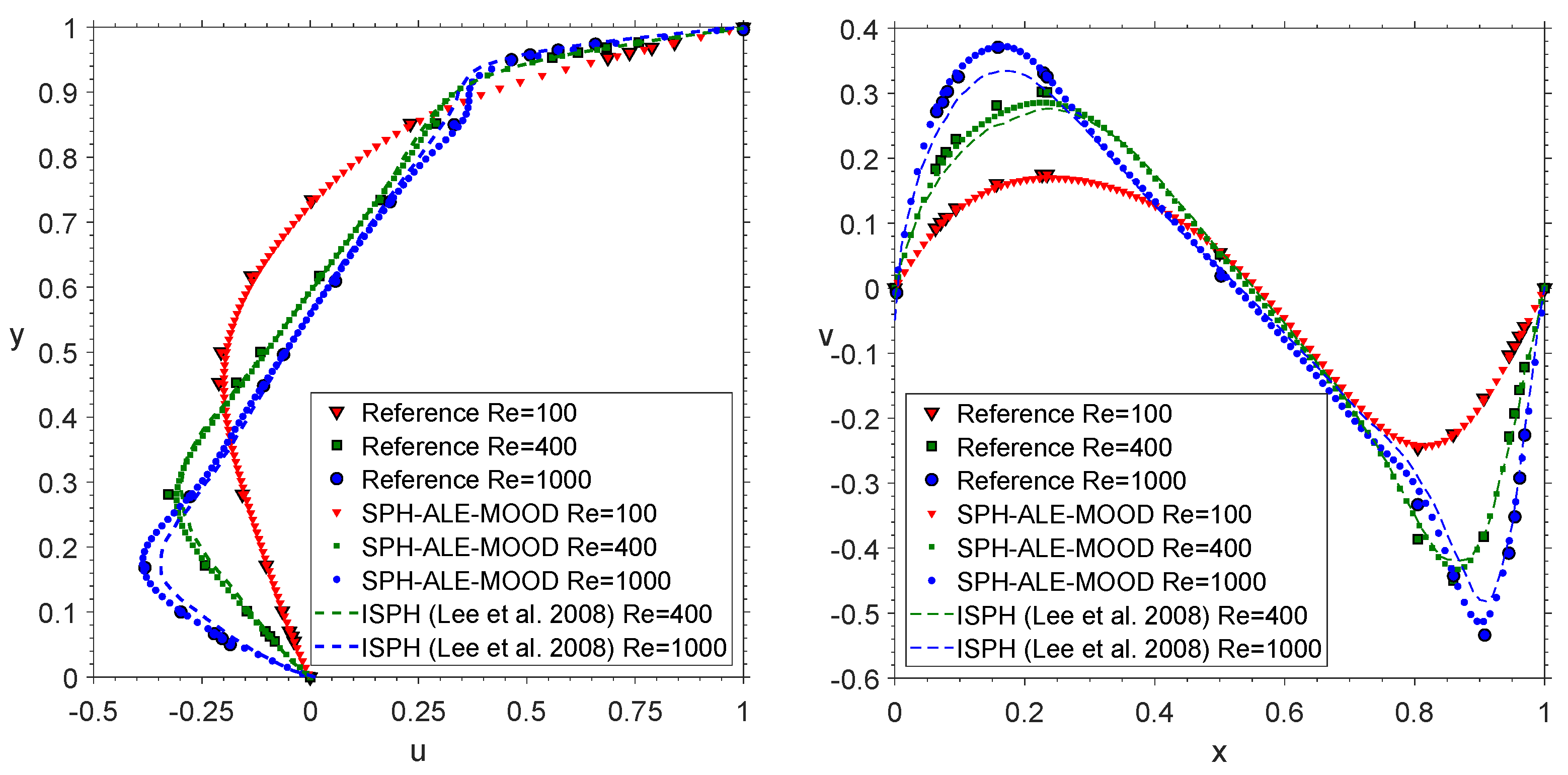
Figure 22 shows the horizontal and vertical velocity profiles along the vertical and horizontal center line for $Re=100$, $Re=400$, and $Re=1000$. Simulations were run for a $t_{final}=500$ s, clearly a time much longer than the one needed to reach the steady-state condition. Results are in good agreement with the reference solution [48] for all the Reynolds number considered. Moreover, the obtained solutions are compared with the ones obtained by Lee et al. [50]. We note that the two schemes use the same number of particles for $Re=400$. For $Re=1000$, the ISPH scheme from [50] uses a finer discretization (${160}^2$ particles).

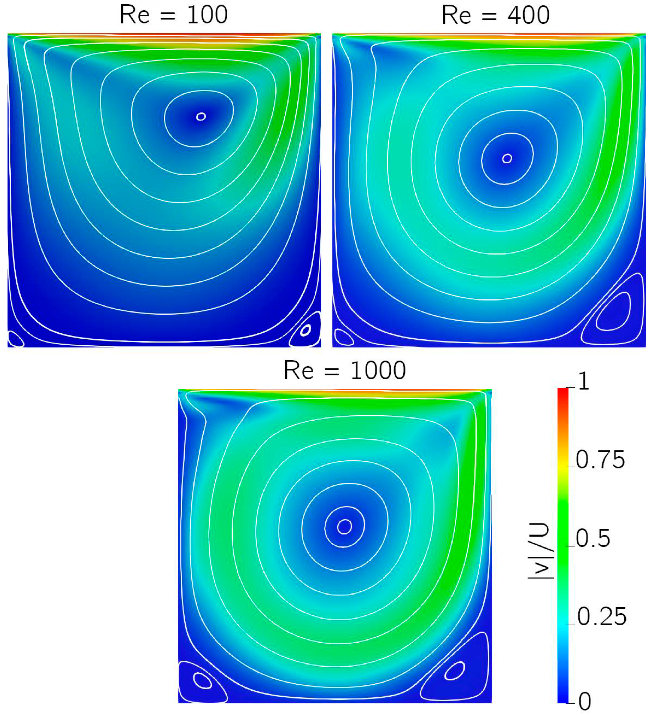
The contours of the velocity magnitude superposed with the streamlines after 500 s are shown in Figure 23. It is seen that the scheme is able to reproduce the primary and secondary vortices of the flow.

6. Conclusions

In this work, we have presented a new high-accurate SPH-ALE method for weakly compressible flow, which can deal with discontinuities. A new approach to compute the viscous flows terms is presented, where Moving Least Squares approximations are used to increase the accuracy and compute the derivatives needed for viscous fluxes. The performance of the proposed scheme is validated with a series of 1D and 2D benchmark problems, and compared with other WCSPH and ISPH schemes from the literature. The proposed method alleviates some of the known drawbacks of weakly compressible schemes. Thus, pressure oscillations are reduced compared with the δ-SPH scheme, and there is no need for an special initialization of the particles. The proposed scheme obtains accurate solutions for any initial distribution of the particles. Moreover, the proposed formulation simplifies the possible combination of the proposed method with grid-based methods (such as the finite volume method, which is closely related to the proposed scheme) or the combination of Eulerian and Lagrangian particles. Even though this issue is not addressed here, it is a very interesting research that will be pursued in forthcoming works.

References

- Violeau, D.; Rogers, B.D. Smoothed Particle Hydrodynamics (SPH) for free-surface flows: Past, present and future. J. Hydraul. Res. 2016, 54, 1–26. [Google Scholar] [CrossRef]
- Ye, T.; Pan, D.; Huang, C.; Liu, M. Smoothed particle hydro-dynamics (SPH) for complex fluid flows: Recent developments in methodology and applications. Phys. Fluids 2019, 31, 011301. [Google Scholar]
- Pu, J.H.; Shao, S. Smoothed Particle Hydrodynamics Simulation of Wave Overtopping Characteristics for Different Coastal Structures. Sci. World J. 2012, 163613, 1–10. [Google Scholar] [CrossRef] [PubMed] [Green Version]
- Vacondio, R.; Altomare, C.; De Leffe, M.; Hu, X.; Le Touzé, D.; Lind, S.; Marongiu, J.-C.; Marrone, S.; Rogers, B.D.; Souto-Iglesias, A. Grand challenges for Smoothed Particle Hydrodynamics numerical schemes. Comput. Part. Mech. 2020. [Google Scholar] [CrossRef]
- Ramirez, L.; Nogueira, X.; Khelladi, S.; Chassaing, J.C.; Colominas, I. A new higher-order finite volume method based on Moving Least Squares for the resolution of the incompressible Navier–Stokes equations on unstructured grids. Comput. Methods Appl. Mech. Eng. 2014, 278, 883–901. [Google Scholar] [CrossRef]
- Nogueira, X.; Ramirez, L.; Khelladi, S.; Chassaing, J.C.; Colominas, I. A high-order density-based finite volume method for the computation of all-speed flows. Comput. Methods Appl. Mech. Eng. 2016, 298, 229–251. [Google Scholar] [CrossRef] [Green Version]
- Cummins, S.J.; Rudman, M. An SPH projection method. J. Comput. Phys. 1999, 152, 584–607. [Google Scholar] [CrossRef]
- Garoosi, F.; Shakibaeinia, A. An SPH projection method. Powder Technol. 2020, 376, 668–696. [Google Scholar] [CrossRef]
- Lind, S.J.; Stansby, P.K. High-order Eulerian incompressible smoothed particle hydrodynamics with transition to Lagrangian free-surface motion. J. Comput. Phys. 2016, 326, 290–311. [Google Scholar] [CrossRef]
- Monaghan, J.J. Simulating free surface flows with SPH. J. Comput. Phys. 1994, 110, 399–406. [Google Scholar] [CrossRef]
- Collé, A.; Limido, J.; Vila, J.P. An accurate multi-regime SPH scheme for barotropic flows. J. Comput. Phys. 2019, 388, 561–600. [Google Scholar] [CrossRef]
- Colagrossi, A.; Bouscasse, B.; Antuono, M.; Marrone, S. Particle packing algorithm for SPH schemes. Comput. Phys. Commun. 2012, 183, 1641–1653. [Google Scholar] [CrossRef] [Green Version]
- Marrone, S.; Antuono, M.; Colagrossi, A.; Colicchio, G.; LeTouzé, D.; Graziani, G. δ-SPH model for simulating violent impact flows. Comput. Methods Appl. Mech. Eng. 2011, 200, 1526–1542. [Google Scholar] [CrossRef]
- BenMoussa, B.; Vila, J.P. Convergence of SPH method for scalar nonlinear conservation laws. Siam J. Numer. Anal. 2000, 37, 863–887. [Google Scholar] [CrossRef]
- Vila, J.P. On particle weighted methods and smooth particle hydrodynamics. Math. Model. Methods Appl. Sci. 1999, 9, 161–209. [Google Scholar] [CrossRef]
- Antuono, M.; Colagrossi, A.; Marrone, S.; Molteni, D. Free-surface flows solved by means of SPH schemes with numerical diffusive terms. Comput. Phys. Commun. 2010, 181, 532–549. [Google Scholar] [CrossRef]
- Krimi, A.; Ramírez, L.; Khelladi, S.; Navarrina, F.; Deligant, M.; Nogueira, X. Improved δ-SPH Scheme with Automatic and Adaptive Numerical Dissipation. Water 2020, 12, 2858. [Google Scholar] [CrossRef]
- Koukouvinis, P.K.; Anagnostopoulos, J.S.; Papantonis, D.E. An improved MUSCL treatment for the SPH-ALE method: Comparison with the standard SPH method for the jet impingement case. Int. J. Numer. Methods Fluids 2013, 71, 1152–1177. [Google Scholar] [CrossRef]
- Avesani, D.; Dumbser, M.; Bellin, A. A new class of Moving-Least-Squares WENO–SPH schemes. J. Comput. Phys. 2014, 270, 278–299. [Google Scholar] [CrossRef]
- Avesani, D.; Herrera, P.; Chiogna, G.; Bellin, A.; Dumbser, M. Smooth Particle Hydrodynamics with nonlinear Moving-Least-Squares WENO reconstruction to model anisotropic dispersion in porous media. Adv. Water Resour. 2015, 80, 43–59. [Google Scholar] [CrossRef]
- Clain, S.; Diot, S.; Loubère, R. A high-order finite volume method for systems of conservation laws Multi-dimensional Optimal Order Detection (MOOD). J. Comput. Phys. 2011, 230, 4028–4050. [Google Scholar] [CrossRef] [Green Version]
- Nogueira, X.; Ramírez, L.; Clain, S.; Loubère, R.; Cueto-Felgueroso, L.; Colominas, I. High-accurate SPH method with Multidimensional Optimal Order Detection limiting. Comput. Methods Appl. Mech. Eng. 2016, 310, 134–155. [Google Scholar] [CrossRef] [Green Version]
- Chiron, L. Couplage et AméLiorations de la Méthode SPH Pour Traiter des éCoulements à Multi-échelles Temporelles et Spatiales. Ph.D. Thesis, Ecole Centrale de Nantes, Nantes, France, 2017. [Google Scholar]
- Oger, G. Aspects Théoriques de la Méthode SPH et Applications à L’hydrodynamique à Surface Libre. Ph.D. Thesis, Université de Nantes and Ecole Centrale de Nantes, Nantes, France, 2006. [Google Scholar]
- Sjah, J. Couplage SPH DEM Pour L’étude de L’érosion Dans les Ouvrages Hydrauliques. Ph.D. Thesis, Ecole Centrale de Lyon, Écully, France, 2013. [Google Scholar]
- Saurel, R.; Cocchi, J.P.; Butler, P.B. Numerical Study of Cavitation in the Wake of a Hypervelocity Underwater Projectile. J. Propuls. Power 1999, 15, 513–522. [Google Scholar] [CrossRef]
- Paillère, H.; Corre, C.; Cascales, J.R.G. On the extension of the AUSM scheme to compressible two-fluid models. Comput. Fluids 2003, 32, 891–916. [Google Scholar] [CrossRef]
- Magoules, F. Computational Fluid Dynamics. In Chapman & Hall/CRC Numerical Analysis & Scientific Computing; CRC Press: Boca Raton, FL, USA, 2011. [Google Scholar]
- Morris, J.P. A study of the stability properties of smooth particle hydrodynamics. Publ. Astron. Soc. Aust. 1996, 13, 97–105. [Google Scholar] [CrossRef] [Green Version]
- Monaghan, J.J.; Lattanzio, J.C. A refined particle method for astrophysical problems. Astonomics Astrophys. 1985, 149, 135–143. [Google Scholar]
- Gallouet, T.; Hérard, J.M.; Seguin, N. Some recent finite volume schemes to compute Euler equations using real gas EOS. Int. J. Numer. Methods Fluids 2002, 39, 1073–1138. [Google Scholar] [CrossRef]
- Bonet, J.; Lok, T.S.L. Variational and momentum preservation aspects of Smooth Particle Hydrodynamic formulations. Comput. Methods Appl. Mech. Eng. 1999, 180, 97–115. [Google Scholar] [CrossRef]
- Dumbser, M.; Zanotti, O.; Loubère, R.; Diot, S. A posteriori subcell limiting of the discontinuous Galerkin finite element method for hyperbolic conservation laws. J. Comput. Phys. 2014, 278, 47–75. [Google Scholar] [CrossRef] [Green Version]
- Marongiu, J.C. Méthode Numérique Lagrangienne Pour la Simulation D’écoulements à Surface Libre-Application Aux Turbines Pelton. Ph.D. Thesis, Ecole Centrale de Lyon, Écully, France, 2007. [Google Scholar]
- Toro, E.F. Riemann Solvers and Numerical Methods for Fluid Dynamics, 3rd ed.; Springer: Berlin/Heidelberg, Germany, 2009. [Google Scholar]
- Ivings, M.J.; Causon, D.M.; Toro, E.F. On Riemann solvers for compressible liquids. Int. J. Numer. Methods Fluids 1998, 28, 395–418. [Google Scholar] [CrossRef]
- Pineda, S.; Marongiu, J.C.; Aubert, S.; Lance, M. Simulation of a gas bubble compression in water near a wall using the SPH-ALE method. Comput. Fluids 2019, 179, 459–475. [Google Scholar] [CrossRef]
- Kundu, P.K.; Cohen, I.; Dowling, D.R. Fluid Mechanics; Elsevier LTD: Oxford, UK, 2015. [Google Scholar]
- Taylor, G.I.; Green, A.E. Mechanism of the production of small eddies from large ones. Proc. R. Soc. Lond. Ser. A Math. Phys. Sci. 1937, 158, 499–521. [Google Scholar]
- Vittoz, L.; Oger, G.; deLeffe, M.; Touzé, D.L. Comparisons of weakly-compressible and truly incompressible approaches for viscous flow into a high-order Cartesian-grid finite volume framework. J. Comput. Phys. X 2019, 1, 100015. [Google Scholar] [CrossRef]
- Sun, P.N.; Colagrossi, A.; Marrone, S.; Antuono, M.; Zhang, A.M. A consistent approach to particle shifting in the δ-Plus-SPH model. Comput. Methods Appl. Mech. Eng. 2019, 348, 912–934. [Google Scholar] [CrossRef]
- Sun, P.N.; Colagrossi, A.; Marrone, S.; Zhang, A.M. The δ-Plus-SPH model: Simple procedures for a further improvement of the SPH scheme. Comput. Methods Appl. Mech. Eng. 2017, 315, 25–49. [Google Scholar] [CrossRef]
- Fourtakas, G.; Stansby, P.K.; Rogers, B.D.; Lind, S.J. An Eulerian–Lagrangian incompressible SPH formulation (ELI-SPH) connected with a sharp interface. Comput. Methods Appl. Mech. Eng. 2018, 329, 532–552. [Google Scholar] [CrossRef]
- Buresti, G. Elements of Fluid Dynamics; Imperial College Press: London, UK, 2012. [Google Scholar]
- Morris, J.P.; Fox, P.J.; Zhu, Y. Modeling low Reynolds number incompressible flows using SPH. J. Comput. Phys. 1997, 136, 214–226. [Google Scholar] [CrossRef]
- Ferrand, M.; Laurence, D.R.; Rogers, B.D.; Violeau, D.; Kassiotis, C. Unified semi-analytical wall boundary conditions for inviscid, laminar or turbulent flows in the meshless SPH method. Int. J. Numer. Methods Fluids 2013, 71, 446–472. [Google Scholar] [CrossRef] [Green Version]
- Fourtakas, G.; Dominguez, J.M.; Vacondio, R.; Rogers, B.D. Local uniform stencil (LUST) boundary condition for arbitrary 3-D boundaries in parallel smoothed particle hydrodynamics (SPH) models. Comput. Fluids 2018, 190, 346–361. [Google Scholar] [CrossRef]
- Ghia, U.; Ghia, K.N.; Shin, C.T. High-Re solutions for incompressible flow using the Navier-Stokes equations and a multigrid method. J. Comput. Phys. 1982, 48, 387–411. [Google Scholar] [CrossRef]
- Szewc, K.; Pozorski, J.; Minier, J.P. Analysis of the incompressibility constraint in the smoothed particle hydrodynamics method. Int. J. Numer. Methods Eng. 2012, 92, 343–369. [Google Scholar] [CrossRef] [Green Version]
- Lee, E.S.; Moulinec, C.; Xu, R.; Violeau, D.; Laurence, D.; Stansby, P. Comparisons of weakly compressible and truly incompressible algorithms for the SPH mesh free particle method. J. Comput. Phys. 2008, 227, 8417–8436. [Google Scholar] [CrossRef]
Figure 1.
Computational domain and kernel support of particle i.
Figure 2.
Stencil for particle i. Interaction between particles i and j represented as a flux in the midpoint interface and one-dimensional moving Riemann problem at the midpoint.
Figure 3.
1D shock tube problem (R1): Pressure and velocity at at time s using 100 particles in the domain m. Results obtained using the SPH base scheme (empty squares) and the SPH-ALE-MOOD method (filled circles).
Figure 4.
1D Sod shock tube problem (T2): Simulations results at s using 200 particles in the domain m. We plot velocity (top-left), pressure (top-right), density (bottom-left), and internal energy (bottom-right). Results obtained using the SPH base scheme (empty squares) and the SPH-ALE-MOOD method (filled circles).
Figure 5.
2D Blast Explosion: Particle initializations. Radial distribution (left), Delaunay distribution (center), Random distribution (right).
Figure 6.
2D Blast Explosion: Density plot in xy domain at time s. Radial distribution (left), Delaunay distribution (center), Random distribution (right).
Figure 7.
2D Blast Explosion: Density profile along radial coordinate at time s. Radial distribution (top left), Delaunay distribution (top right), Random distribution (bottom).
Figure 8.
Taylor–Green vortex: Schematic representation of the computational domain and streamlines.
Figure 9.
Taylor Green flow: Layout of the particles. Hollow red circles: ghost periodic particles. Solid blue circles: fluid particles.
Figure 10.
Taylor Green flow: Results for at . Left: u-velocity field; center: v-velocity field: right: pressure field.
Figure 11.
Taylor Green flow: Comparison of the numerical and theoretical decay of the kinetic energy factor defined in Equation (15) (left) and the maximum velocity (right) for , and .
Figure 12.
Taylor Green flow: Comparison of the time evolution of the pressure at the center of the domain for (left) and (right).
Figure 13.
Taylor Green flow: Comparison of the pressure field along for .
Figure 14.
Taylor Green flow: Computational costs for different particle discretization.
Figure 15.
Couette and Poiseuille Flows: Schematic representation of the problems.
Figure 16.
Couette and Poiseuille Flows: Particle layout (left). Schematic representation of the antisymmetric technique for wall ghost particles (right).
Figure 17.
Time evolution of the velocity profile for the Poiseuille flow with Eulerian (left) and Lagrangian description (right). The numerical solution is compared with the exact solution presented in (18).
Figure 18.
Time evolution of the velocity profile for the Couette flow (top left), (top right), (bottom left), and (bottom right). The numerical solution is compared with the exact solution presented in Equation (17).
Figure 19.
Convergence analysis for the Couette flow at (left) and at (right).
Figure 20.
2D Lid-driven cavity flow: Schematic representation of the geometry and boundary conditions.
Figure 21.
2D Lid-driven cavity flow: Layout of the particles and treatment of ghost particles in corners.
Figure 22.
2D Lid-driven cavity flow: On the left, horizontal velocity component u along L for , , and . On the right, vertical velocity component v along L for , , and .
Figure 23.
Contours of velocity and streamlines for lid driven cavity at different numbers. (top left), (top right), and (bottom).
Publisher’s Note: MDPI stays neutral with regard to jurisdictional claims in published maps and institutional affiliations. |
© 2021 by the authors. Licensee MDPI, Basel, Switzerland. This article is an open access article distributed under the terms and conditions of the Creative Commons Attribution (CC BY) license (http://creativecommons.org/licenses/by/4.0/).
Share and Cite
MDPI and ACS Style
Eirís, A.; Ramírez, L.; Fernández-Fidalgo, J.; Couceiro, I.; Nogueira, X. SPH-ALE Scheme for Weakly Compressible Viscous Flow with a Posteriori Stabilization. Water 2021, 13, 245. https://doi.org/10.3390/w13030245
AMA Style
Eirís A, Ramírez L, Fernández-Fidalgo J, Couceiro I, Nogueira X. SPH-ALE Scheme for Weakly Compressible Viscous Flow with a Posteriori Stabilization. Water. 2021; 13(3):245. https://doi.org/10.3390/w13030245
Chicago/Turabian StyleEirís, Antonio, Luis Ramírez, Javier Fernández-Fidalgo, Iván Couceiro, and Xesús Nogueira. 2021. "SPH-ALE Scheme for Weakly Compressible Viscous Flow with a Posteriori Stabilization" Water 13, no. 3: 245. https://doi.org/10.3390/w13030245
Note that from the first issue of 2016, this journal uses article numbers instead of page numbers. See further details here.