
Optical Methods for River Monitoring: A Simulation-Based Approach to Explore Optimal Experimental Setup for LSPIV


Dipartimento di Ingegneria, Università degli Studi di Palermo, Viale delle Scienze, Ed. 8, 90128 Palermo, Italy
*
Author to whom correspondence should be addressed.
Water 2021, 13(3), 247; https://doi.org/10.3390/w13030247
Submission received: 22 December 2020
/
Revised: 15 January 2021
/
Accepted: 17 January 2021
/
Published: 20 January 2021
(This article belongs to the Section Hydrology)
Abstract
:Recent advances in image-based methods for environmental monitoring are opening new frontiers for remote streamflow measurements in natural environments. Such techniques offer numerous advantages compared to traditional approaches. Despite the wide availability of cost-effective devices and software for image processing, these techniques are still rarely systematically implemented in practical applications, probably due to the lack of consistent operational protocols for both phases of images acquisition and processing. In this work, the optimal experimental setup for LSPIV based flow velocity measurements under different conditions is explored using the software PIVlab, investigating performance and sensitivity to some key factors. Different synthetic image sequences, reproducing a river flow with a realistic velocity profile and uniformly distributed floating tracers, are generated under controlled conditions. Different parametric scenarios are created considering diverse combinations of flow velocity, tracer size, seeding density, and environmental conditions. Multiple replications per scenario are processed, using descriptive statistics to characterize errors in PIVlab estimates. Simulations highlight the crucial role of some parameters (e.g., seeding density) and demonstrate how appropriate video duration, frame-rate and parameters setting in relation to the hydraulic conditions can efficiently counterbalance many of the typical operative issues (i.e., scarce tracer concentration) and improve algorithms performance.

1. Introduction
River discharge data availability is of crucial interest for a variety of practical hydrological applications, such as the implementation, calibration and validation of hydrological models for water resources assessment and management [1,2], the monitoring of climate change impacts on water resources and runoff extremes [3], the identification of the best criteria for the hydraulic infrastructures design and evaluation, the strategic planning and policies developing for both civil protection and water management activities.
In many practical applications, discharge estimation in natural rivers is conducted through a velocity-area method, based on: (i) the discrete point sampling of flow velocity along transects in a specific cross section of interest; (ii) the derivation of both average flow velocity and associated wetted area [4,5,6]. This approach traditionally involves the use of current meters, requires a large employment of highly specialized personnel, and it is extremely expensive and time-consuming. Multiple field campaigns are often conducted on the same cross-section of a river with the ultimate objective of deriving the flow rating curve, which requires a consistent dataset of paired measures of discharge and river stage, with a consequent need of field campaigns conducted in different periods of the year in order to ensure a good flow regime representativeness. Moreover, cross sections may vary over time due to vegetation growth and river-bed movements [7], and this implies the need for frequent replications of the field campaigns and periodic flow rating curve recalibrations.
Errors in river stage and velocity measurements during surveys have been regarded as considerable sources of uncertainties in discharge measurements using rating curves [8,9]. Moreover, these last are rarely adequate to evaluate discharge under severe flood conditions [10] when extrapolation is often necessary. This last aspect is related to the difficulties in sampling discharge-stage couples under high flow conditions with traditional approaches and instruments, especially due to the increased safety risks for operators.
Although different and valid options are often considered, from the use of Doppler instrumentation [11] to radar [12,13] and remote sensing observations [14], these rarely reduce the problems related to both expensive equipment and need for prolonged and laborious field campaigns through expert personnel. There is an increased awareness that advances in flow monitoring towards easier and more accessible methods, allowing for higher spatial and temporal resolution, are still urgently needed.
Optical based techniques offer a great potential for river monitoring [15], allowing for massive, easy and low-cost acquisitions of a wide range of measures in real time, at any flow conditions and at high spatial resolution. Such techniques are rapidly evolving also in consideration of the increasing availability of a new generation of optical sensors, digital cameras and methodologies. Recent years have been witnessing in fact a significant development of monitoring methods based on the elaboration of sequences of images captured by digital permanent gauge-cams installed close to the river, mobile-devices with operators standing on the banks and on bridges, or even cams installed on unmanned aerial vehicles (e.g., [16,17]).
Among the various image-based methods (e.g., [18,19,20,21,22]), two different approaches have gained wide consensus for natural rivers monitoring: the large-scale particle image velocimetry (LSPIV) and particle tracking velocimetry (LSPTV) techniques. Both techniques, based on the analysis of floating tracers, were originally developed for laboratory experiments under controlled conditions and essentially enlarge the basic technique principles of the particle image velocimetry (PIV) and particle tracking velocimetry (PTV) technique to the large-scale cases; LSPIV adopts a Eulerian point of view, while LSPTV uses a Lagrangian point of view. The two techniques have several common characteristics, described for instance in [23,24], while the main differences lay in the adopted procedures for the evaluation of the recordings: LSPIV estimates the velocity at image sub-regions, while LSPTV reconstructs the trajectory of individual particles transiting in the field of view [15].
The surface velocity field is indirectly obtained by measuring the velocity of floating tracer particles, naturally present or artificially introduced to the flow, which is assumed to move with the local flow velocity. The dynamics of the liquid surface are recorded by cameras, through a sequence of consecutive frames, reconstructing the local flow velocity starting from the identification of the tracer particles displacements between pairs of subsequent frames. Differently from the LSPTV, the here used LSPIV subdivides all frames into small regular sub-regions, called interrogation areas (IAs); local distribution patterns and the displacements are usually determined by cross-correlating the IAs of consecutive frames.
Measurements with LSPIV technique typically include the following four main phases:
- “seeding”, i.e., introduction of tracer with adequate geometry and density in a well-lit area of the river, using particles that accurately describe the motion of the river, not interfering significantly with it; this is needed only if the characteristics of naturally occurring flow tracer are not appropriate for the scope (e.g., scarce concentration with non-uniform dispersion, inadequate dimensions, etc.);
- “recording”, i.e., recording of images with an adequate temporal resolution;
- “processing”, i.e., elaboration of recorded images, also including pre-processing procedures (e.g., images stabilization, orthorectification and manipulation to increase tracer brightness and the contrast between tracers and water) if needed, and estimation of the tracer displacements between pairs of consecutive images;
- “evaluation”, i.e., velocity data post-processing to characterize the velocity field over the entire area of interest.
The estimation of the discharge is also possible by combining the bathymetry of a river cross section with the calculated surface velocity field and adopting simplified hypotheses on vertical velocity profiles [25].
Monitoring approaches based on LSPIV pattern recognition technique show several advantages with respect to traditional methodologies. First of all, the simplicity: field campaigns are easier, faster and do not require personnel with specific skills; instruments are not submerged in the stream, limiting flow disturbance and, during floods, possible damages and risks for operators. Secondarily, the affordability: recent technological advancements have allowed commercially-available and inexpensive cameras for high resolution capabilities and equipment for extensive image storage and processing. Many software programs, based on LSPIV and LSPTV, are also widely available, user-friendly and freely available, such as FlowManager [26], RIVeR [27], FUDAA-LSPIV [28,29]. Despite the numerous and important advantages, image-based river flow monitoring is still rarely adopted in practical applications. The lack of consistent image acquisition and processing protocols feeds the urgent need for in-depth analyses that could offer, in the near future, the possibility of systematically implementing such methods in practical applications according to appropriate operational standards.
This work moves exactly along this direction, and it is aimed to analyze performance and sensitivity of a free and popular software based on PIV to the main factors, which typically influence the technique. In particular, an Image Sequence Generator (ISG) has been implemented ad-hoc with the aim to create, under fixed parametric scenarios, several replications of synthetic sequences of images with known and uniformly distributed tracers moving according to a known and stationary surface velocity profile simulating two possible flow velocity conditions (slow and fast).
The selected software for the analysis is PIVlab [30], an open-source tool of MATLAB, which recently gained considerable attention for natural river flow monitoring (e.g., [15,31]). All the sequences generated by the ISG for each scenario are then processed in PIVlab, statistically analyzing the results, with particular emphasis on the error in the estimation of the surface velocity field characteristics.
The work is structured in two parts. The first considers a set of simulations dedicated to the analysis, for fixed number of processed frames, of the impact of different tracer characteristics under various flow velocity and environmental conditions. With regard to this last aspect, two alternative hypotheses are considered with the aim to investigate the influence of possible disturbances typical of environmental conditions. Some of the aspects investigated in the first set of simulations have been recently explored by [32] with regard to the LSPTV technique (i.e., using PTVlab software [33]). Differently from other existing synthetic studies on optical methods (e.g., [32,34,35]), here, a realistic distribution of the flow velocity along the cross-section is considered.
The second part is constituted by simulations entirely focused on the role of the selected number of frames which depends on the selected duration of the video sequences and the frame elaboration frequency (frame-rate).
In real applications, the video duration should depend on different factors (e.g., tracer visibility and seeding density/dispersion characteristics in time, flow and illumination conditions and variability, etc.) and it is rather usual to acquire an overabundant sequence of images from which only a limited and representative subset is extracted and processed. The frame-rate of acquisition depends on the adopted device for recording. For instance, Charge-Coupled Devices, used in laboratory PIV experiments, can acquire video with frame-rate over 1000 fps. Commercial cameras, often used for LSPIV applications, typically record with frame-rate around 24–30 fps, while recent high-speed cameras acquisition frequency can reach up to about 250 fps. Many software for PIV analysis allow for modifying the processing frame-rate with respect to the frame-rate of acquisition. A high frame-rate could imply an excessively low frame-by-frame tracer displacement, especially under slow flow conditions, while the adoption of low frame-rate, especially under fast flow conditions, could imply excessive displacements, greater than the IA, with consequent loss of correlation due to in-plane motion [36]. Both situations have to be avoided, since they negatively affect optical matching algorithms. The second set of simulations in this study is thus aimed to provide some indications about the choice of the frame-rate and the processed video sequence duration depending on the local flow velocity.
A general drawback in the full evaluation of the performances offered by software programs based on optical techniques is the absence of benchmarks, since current meter or Doppler measurements are not appropriate for massive comparing observations; for this reason, a synthetic image-based approach represents the only way to fully characterize a specific algorithm. This paper critically explores strengths and weakness of PIVlab capabilities and capitalizes our best present knowledge on this technique. Results of this work may be useful, on the one hand, in identifying possible source of errors in flow velocity estimations by LSPIV based methods and, on the other hand, in identifying the optimal experimental setup under different environmental circumstances. The numerical approach proposed could be used, for example, to preliminarily verify the operability of LSPIV on a given site. Information arising from our analyses could be useful in defining criteria and guidelines for practical applications.
2. Materials and Methods
2.1. PIVlab Software
PIVlab software, developed by the Energy and Sustainability Research Institute of Groningen, the Netherland [30], is a free, open-source tool for performing digital PIV flow analysis in MATLAB environment. Apart from a very user-friendly graphical user interface, the program is accessible from the command line of MATLAB and this offers the possibility to easily automate the whole process, to include it in other applications and, in general, to benefit from all the MATLABs extensive plotting and data handling features.
PIVlab allows for importing image sequences and to choose the processing style between two available modes: type 1 (i.e., 1-2, 2-3, 3-4, etc.), so that the second image of each analyzed pair of images is also the first of the successive one; type 2 (i.e., 1-2, 3-4, 5-6, etc.), so that the cross-correlation analysis is applied only once per each image.
The typical PIVlab workflow consists of three main steps: (1) pre-processing; (2) image evaluation; (3) post-processing. The tool offers, in fact, various pre-processing techniques to enhance images quality and help tracers’ recognition (i.e., histogram equalization, intensity high-pass and intensity capping).
With regards to the images evaluation step, PIVlab provides the possibility to choose between two different correlation algorithms: D-CC (Direct Cross-Correlation) and FFT-CC (Fast Fourier Transform Cross-Correlation). Both are based on a cross correlation of small sub-images (interrogation areas, IAs) of an image pair. The former computes the correlation matrix between corresponding IAs in the spatial domain. The location of the intensity peak in the correlation matrix provides the most probable displacement of the particle from the first to the second IAs. With this approach the corresponding IAs in the two paired images can have different sizes. With the FFT-CC approach, which conversely uses IAs of identical size, the correlation matrix is computed in the frequency domain using FFT. Although the second approach has been demonstrated to create less accurate results than the D-CC [37], especially when flow motion is not unidirectional, it reduces significantly the computational cost, especially when large IAs are considered, which actually is a very relevant drawback of D-CC. Moreover, the accuracy of the FFT can be offset by running several passes on the same dataset [38] according to a methodology described in [30] and based on a window deformation interpolator, using either a linear interpolation (faster) or a spline interpolation (higher precision, but slower).
The location of the intensity peak of the correlation matrix, which determines the displacement of IAs, can be refined with sub-pixel precision by using one of the two peak finding algorithms implemented in PIVlab: (i) 2·3-point fit and (ii) 9-point fit. The first consists in fitting two times a one-dimensional Gaussian (3-point fit) to the integer intensity distribution of the correlation matrix for both x and y axes independently, while with the second, a two-dimensional Gaussian function (9-point fit) is used.
Finally, the post-processing phase includes three steps: (i) filtering velocities and removing possible outliers; (ii) replacing missing vectors through a data interpolation technique based on a boundary value solver for interpolation; and, finally, (iii) removing measurements noise by applying a data smoothing technique based on a penalized least squared method [39]. For further details on PIVlab, interested readers may refer to the original paper [30].
Modelling Framework and PIVlab Setup
In order to allow for a statistical characterization of the results, several sequences for each considered scenario were created and processed; different scenarios were analyzed, leading to a wide number (i.e., 5200) of image sequences to be processed. This highlights the need for exploiting a not computational expensive automatic procedure.
For this reason, despite PIVlab presents a very user-friendly GUI, in this work it was used through MATLAB command lines; the image processing by PIVlab was used as the core of an opportunely implemented modeling chain, schematically reported in Figure 1, that also contains a code for the preliminary creation of the image sequences to be processed with the Image Sequence Generator—ISG (see Section 2.2) and a code for the subsequent post-processing of PIVlab estimates to automatically achieve the desired indicators (Results Analysis and Visualization—RAV see Section 2.3). Such modules have been separately developed in MATLAB and then fully integrated with PIVlab script.
PIVlab is forced with the output of the ISG. Since each sequence is formed by synthetically generated images, no pre-processing procedure is required by PIVlab. The adopted mode for the sequence processing style is type 1 (i.e., 1-2, 2-3, etc.) which, although more time consuming, is more performing than the alternative type 2 (i.e., 1-2, 3-4, etc.) for cases of sequences with a low frame-rate.
In order to reduce the calculation times, the FFT-CC algorithm was preferred to the D-CC, adopting the needed precautions to maintain an adequate accuracy of the results. In particular, three passes were set, using linear interpolation option as window deformation interpolator.
The width of the 1st pass IAs was selected by imposing three criteria suggested by PIVlab developers: (i) not lower than 50% of the minimum frame dimension; (ii) lower than the minimum frame dimension; (iii) higher than two times the maximum presumable frame-by-frame particle displacement. It is, in fact, desirable that the displacement of the particles remains within both the corresponding IAs of the image pair. The width of the 1st pass IAs was then set equal to 400 px (pixel) in consideration of the following aspects, which will be deepened in the following paragraphs: (i) squared frames of 600 × 600 px were generated; (ii) a maximum frame-by-frame displacement of 161 px was considered, i.e., the tracer displacement corresponding to the maximum velocity in the midstream for the fast velocity case and for frame-rate of 4 fps (frame per second).
The width of IAs for the following passes was obtained by halving the width relative to the previous pass, i.e., 200 and 100 px for the 2nd and 3rd pass, respectively. This setup allows the processing algorithm to create a grid of 11 × 11 computational nodes over the frame, with a total of 121 equidistant nodes placed at a distance of 50 px with each other and from the edges of the frame.
The results obtained by the cross-correlation algorithm application to each replication of a given scenario are point velocity vectors, computed node by node in the entire computational grid. Such data are then passed to the post-processor RAV by which: (i) all the results of interest at the level of single sequence per scenario are computed and stored; and (ii) a statistical analysis is carried out on the entire set of sequences per scenario, computing the main descriptive statistics and creating corresponding box-plots and tables.
2.2. Image Sequence Generator
An Image Sequence Generator (ISG) has been coded in MATLAB and implemented ad hoc for the scopes of this work. The code, after an opportune setup, is able to generate a desired number of synthetic image sequences, simulating a floating tracer moving under controlled conditions according to two different and alternative operational modalities: (1) ideal environmental condition (ID), by which the model reproduces a tracer moving on a black background; (2) semi-real environmental condition (SR), by which the tracer moves on a real background. In this last case, an actual image from a real river, representative of clear water conditions, is used as further input to the ISG.
Floater is simulated with disks of regular geometry having a uniform white color that, in the case of SR, is altered with white noise. The ISG creates tracers under two different modalities: CON (constant size) and VAR (variable size). In the CON case the particles have a uniform circular shape with a fixed diameter, while in the VAR case the disks have been generated with a diameter variable according to a Gaussian distribution with fixed parameters. Tracer is randomly distributed with a uniform concentration, according to a Poisson distribution with parameter λ (seeding density), on the grid lattice representing the background.
Once the grid lattice with the floating tracers is generated, a unidirectional motion is imposed to the floaters according to a realistic cross-section velocity profile that accounts for flow velocity reduction near the banks due to frictional forces. In particular, the model requires to impose a normalized velocity cross profile, which have to be multiplied by the desired mean flow velocity. A specific part of the code was implemented in order to exclude the possibility of particles’ overlap. Each particle keeps constant properties (i.e., shape and size) along its motion and results simply shifted from a frame to the next one.
The ISG setup includes the setting of different parameters (Figure 2). Considering the purposes of this work, it has been decided to keep some of these as constants over the different scenario, such as the frame dimension, the spatial resolution, the normalized cross-section flow velocity profile and the number of replications generated for each scenario. Then, the sensitivity of PIVlab to the remaining parameters has been explored by varying them according to a wide range of combinations.
In particular, four different schemes have been created combining the two environmental conditions (i.e., ID and SR) with the two alternative hypotheses for the tracer size (CON and VAR): ID-CON, ID-VAR, SR-CON, SR-VAR.
A first set of simulations has been carried out for all the aforementioned schemes, creating scenarios with sequences of fixed time duration and frame-rate under six different configurations, obtained by combining two flow velocity profiles (S = slow; F = fast) and three different seeding densities per frame (LD = low; MD = medium; HD = high). A second set of simulations has been carried on scenarios obtained by varying alternatively the frame-rate first (with fixed sequence duration) and, then, the sequence duration (with fixed frame-rate). These scenarios have been created considering only the ID-CON scheme and two seeding density-velocity configurations (MD-S and MD-F).
The different combinations of schemes and configurations for each set of simulations have generated a total of 52 different scenarios, as schematically represented in Table 1. Some demonstrative synthetic image sequences are provided in the Supplementary Materials.
ISG Setup
For the setting of the parameters under the different scenarios we referred to other works already present in literature and field observations (e.g., [24,29,33,35,40,41,42,43]). The parameters used in this work are synthesized in Table 1.
In particular, a wide frame dimension (i.e., 600 × 600 px) was set since, as it will be discussed later, only a limited portion, centered in the middle of the image, will be used for avoiding possible disturbances in the contour region, i.e., border effects [32].
For the generation of the grid lattice under the SR schemes, an actual image, which has been acquired and orthorectified (no other pre-processing procedures have been applied) during a past streamflow monitoring field campaign at the Oreto river (Italy) in 2018, has been used. This image was considered ideal for the scope since it was acquired in a perfect vertical condition by drone, hovering in stable position at 10 m above the river surface, under optimal daylight and clear water conditions. However, it is worth noting that the use of static background for the dynamic generation of a video sequence does not allow to include in the analysis some possible sources of error, neglected in this study, which usually occur in field conditions, such as the effects of glare and shadows or light intensity variation associated with free-surface deformations. The same spatial resolution of the image (i.e., 0.003 m/px), which is also similar to that adopted in [35], was set in the ISG for the generation of all the synthetic sequences. For each scenario it has been decided to perform various replications, generating 100 independent sequences with the same parameter set, in order to allow for a statistical characterization of the results.
A unidirectional and stationary motion was imposed to the particles according to a synthetic and symmetric cross-section flow profile (Figure 3). A reference profile was first derived starting from the results of field campaign in a real river [44], retrieving experimental points for half section, formed by pairs of distance from the bank (normalized with respect to the total length of the cross-section) and the corresponding surface velocity, measured by the ADCP technique. Different functions were fitted to the experimental points, and the best fitting curve was found by a logarithmic function (R2 = 0.985), which actually is one of the most widely used to characterize the horizontal velocity profile with the distance from the bank [45], even if it does not account for possible effects of turbulence which could strongly influence real profiles.
The final normalized profile for the entire section, whose equation is reported in Figure 3, was obtained by: (i) reflecting the obtained fitting function across the central axis of symmetry and (ii) rescaling the function so to obtain a unit average velocity. The obtained profile, characterizing the velocity (normalized with respect to the average velocity uavg) distribution as a function of the normalized distance from the right bank (drb/drb,max), was finally used to generate the slow (S) and the fast (F) transverse velocity profiles, setting the average velocity uavg equal to 0.5 m/s and 1.5 m/s for the velocity conditions S and F, respectively. The corresponding average frame-by-frame particle displacements, assuming a frame-rate of 4 fps, are equal to 42 px (S) and 126 px (F), with values ranging from about 32 px (S case close to the banks) to about 161 px (F case in the midstream).
In the CON case all the particles are characterized by a fixed diameter of 10 px, while in the VAR case the disks have different size, with diameters randomly ranging from 2 to 20 px, generated from a Gaussian distribution with mean and standard deviation equal to 10 and 3 px, respectively. The selected mean diameter of 10 px is rather common for both laboratory and field scales experiments [32,35,42], since it is sufficiently large to avoid peak locking effects [40,41] and, at the same time, consistent with typical dimensions of tracers used in real applications [22]. Under the ID schemes, the disks have a uniform white color, while, under the SR, the color was altered, frame by frame, by a white noise with standard deviation of 0.05 in order to simulate environmental signal noises, following the same approach used in [32]. Figure 4a shows an example of tracers for four possible schemes ID-CON, ID-VAR, SR-CON and SR-VAR.
Moreover, for the choice of the seeding density, we referred to other works in literature (e.g., [32,43]) creating images with Poissonian distributed tracers, with parameter λ (corresponding to the mean seeding density for frame) equal to 6.4 × 10⁻⁵ ppp (particles per pixel) for the case LD, 2.5 × 10⁻⁵ ppp for the MD and 1.3E-03 ppp for the high density case (HD). Considering the selected size of the frame and mean diameter of the particles, the imposed seeding densities imply an average percentage of pixels with tracer over the entire frame of 0.5%, 2% and 10% of the frame, with a mean occurrence of 23, 91 and 459 disks per frame, for the LD, MD and HD cases, respectively. The explored seeding density range takes into account two limit cases: (i) the LD case could be considered as a lower limit, below which the matching algorithm could have problems related to frame regions with scarce or null presence of tracer; (ii) the HD case could be representative of an upper limit seeding density condition, over which individual particles could start forming clusters, causing a possible increment of the measuring uncertainties [46]. In Figure 4b an example for each case under the ID-CON scheme is reported.
For the first set of simulations, we have set a constant frame-rate of 4 fps, and sequence duration equal to 30 s. Such settings provide a suitable displacement of particles between image pairs for both S and F velocity cases and ensure a number of processed frames (nFR) equal to 121 frames for each sequence and sufficient for a consistent characterization of the surface velocity field, limiting at the same time the associated computational times. Nevertheless, the second set of simulations was addressed to investigate the importance of the number of analyzed frames. With this aim, first the sequence duration was fixed equal to 30 s, altering the frame-rate (considering 2, 3, 4, 6, 8, 12 and 16 fps), and then, the frame-rate was fixed equal to 4 fps, considering different sequence durations (d = 5, 15, 30, 45, 60, 90 and 120 s), i.e., processing then a total number of frames ranging from nFR = 21 (for d = 5 s) to 481 frames (for d = 120 s).
2.3. Results Analysis and Visualization (RAV) Module
Although PIVlab offers a full suite of tools for results analysis and visualization, since in this work a considerable number of synthetic image sequences have to be managed, it has been preferred to create a specific MATLAB script, named Results Analysis and Visualization (RAV), dedicated to the analysis and the statistical characterization of the results relative to each parametric scenario.
For each sequence, the estimated field of surface velocity is simply represented in a matrix form by a colored “heat map”, reporting the point velocity at any grid node.
A matrix, reporting the Absolute Percentage Error, APEi (where i refers to the generic i-th node), has been associated to each sequence. The APEi values arises from the comparison at each computational grid node between the surface velocity estimated by PIVlab () and the velocity imposed in the ISG (), and are computed as:
Once the actual analysis area is selected, the script associates to each sequence an index, named MAPE (Mean Absolute Percentage Error), that is the mean of all the APEi over the analyzed area:
where n refers to the total number of computational nodes within the analyzed area.
For each scenario, the script creates box-plots of all the MAPE values for the 100 corresponding realizations, with indications about the median, the interquartile range (IQR), the most extreme data points not considered outliers (whiskers) and the outliers (red marks). Moreover, it also generates maps reporting, again as colored heat map, the node-by-node mean values of the APEi over the 100 replications (<APEi>). Finally, for a reference cross-section transect within the analysis area (i.e., the central one), and for a given scenario, the script creates a comparison graph between the cross-section velocity profiles imposed by the ISG and that estimated by PIVlab; this last is displayed in the form of box-plots of the 100 surface velocity values estimated at each node of the transect for each replication of given scenario.
3. Results
3.1. Simulations with Equal Number of Processed Frames
The first set of simulations refers to 24 scenarios obtained differently combining the six possible density-velocity configurations (i.e., the LD, MD and HD density with the S- and the F-velocity cases) and the four environmental condition-tracer size schemes (i.e., ID-CON, ID-VAR, SR-CON and SR-VAR). All the synthetic sequences generated for this phase of analysis simulate a video sequence with fixed duration of 30 s and frame-rate of 4 fps.
3.1.1. Border Region and Selection of the Actual Area of Analysis
The frame was initially entirely selected as area of analysis, thus considering a computational grid consisting of a total of 121 computational nodes arranged on 11 horizontal rows (along the flow direction) and 11 vertical columns (here referred as transects and representative of cross-sections orthogonal to the flow direction); the aim of this type of analysis is to investigate possible frame-border effects and to identify the region of the frame not significantly affected by frame-border effects.
The results in terms of <APEi> maps are reported, only for scenarios under the ID-CON scheme, in Figure 5 for the S (top panels) and F (bottom panels) cases and the LD (left panels), MD (middle panels) and HD (right panels) scenarios. From the figure, it can be noticed how border effects for the S cases are less evident than for the F cases. High displacements and low seeding density concur in the reduction of the number of paired particle images that appear in both IAs of an image pair, especially in the input (left edge of the frame) and output (right edge of the frame) zones, generating loss of correlation with higher uncertainties in the reconstruction of surface velocity field.
Significantly high values of <APEi> (up to 34%) were found for the LD-F cases, while, in general, the values of <APEi> decrease with decreasing velocity and with increasing seeding density (Figure 5). For the best case, which corresponds to HD-S (lowest <APEi>), the borders with the highest errors are only at the top and the bottom of the frame, where <APEi> are always below 15%; in this case, the dominant source of error is the presence of out-of-plane velocity gradients, which are higher approaching the banks and could cause errors in the measured in-plane velocity components due to the finite number of particles within a IA and their random positions.
Figure 5 shows how, except for the two LD cases (LD-S and LD-F), errors are mainly concentrated in the border region, especially in the tracer output zone (right border) and at the corners of the frame, which suffer loss of correlation due to both in-plane motion and out-of-plane velocity gradients. For all the configurations with MD and HD, it is possible to identify a wide zone in a central part of the frame (see the areas delimited by the red contour in Figure 5) where the values of <APEi> are never above 2% and 3% for the cases S and F, respectively. This region, selected as area of investigation, will be used as region of interest for all the successive analyses; it includes the 5 central transects (progressively named along the flow direction, from T1 to T5), with 7 nodes along each transect (progressively named from the top, R1, to the bottom of the frame, R7), covering a total of 35 computational nodes within an area of 250 × 350 px. The dashed black vertical line in the graphs of Figure 5, corresponding to the central transect T3, is selected as the reference transect to compare estimated and imposed cross-section velocity profiles. It is worth emphasizing that the consideration of a reduced central portion of the frame as area of investigation, implies that the imposed velocity profile for the region of interest is characterized by a mean velocity slightly higher than that imposed in the ISG module, which refers to the entire frame (0.59 vs. 0.5 m/s for S case and 1.76 vs. 1.5 m/s).
The low seeding density cases (LD-S and LD-F) in Figure 5 show a behavior rather different from the other cases due to an insufficient number of tracers, which frequently leads to many empty IAs, reducing the probability for detective valid displacements and producing loss-of-pairs [47]. The effect of loss-of-pairs in the tracers output zone (right border) enlarges to the entire map for the LD-F case, with consistent <APEi> in all the computational grid and errors in the central parts of the frame even higher than those at the top and bottom edges of the frame. The analysis of the correlation levels shows that the correlation peaks in the output tracer zone are broadened and with a strongly reduced intensity; this loss of correlation is probably due to the fact that some particles leave the IAs because, for the F velocity, in-plane displacements are large with respect to the selected IA size. However, for both LD-S and LD-F cases, the values of <APEi> within the actual area of analysis, although consistently higher than for the other two seeding density cases, remain in a range significantly lower than the <APEi> in the excluded border region; for instance, for the LD-S, the mean value and the standard deviation of the <APEi> in the area of analysis are equal to 4.1% and 1.8%, respectively, while the corresponding values for the excluded border region are 8.6% and 7%, respectively.
3.1.2. Evaluation of the Surface Velocity Field
For almost all the processed sequences, PIVlab revealed a satisfying accuracy in reproducing the imposed surface velocity field, also demonstrating an acceptable stability (low uncertainty) of results among the different realizations for given scenario. Actually, the software failed only for the LD-F configuration, when the estimated error for many sequences was, on average, one order of magnitude higher than for the other cases with higher seeding density.
The best case in Figure 6 (top panels) refers to the HD-S case which has a MAPE value below 0.6% and it is strongly consistent with all the values obtained for the other sequences under this configuration. The surface velocity field is well reconstructed within the entire area of analysis, with similar velocity profiles for the different transects. The map of APEi shows homogeneous distribution of the errors, with slightly higher values (up to 1.9%) concentrated at the nodes along the midstream row (i.e., R4). For all the other nodes of the actual area of analysis, APEi are below 0.9%.
PIVlab sensitivity to the seeding density in relation to the flow velocity conditions is shown in Figure 7, through a comparison between maps of APEi for representative cases of the opposite configurations LD and HD, under the ID-CON scheme and for both S and F cases. Similarly, the role of the investigated environmental condition (ID vs. SR) and tracer size (CON vs. VAR) parameter set is highlighted in Figure 8 for representative cases with equal seeding density (i.e., the MD). For each scenario reported in Figure 7 and Figure 8, the replication with the median MAPE has been selected as representative case.
Figure 7 confirms that errors for the LD cases are significantly higher than those of the HD cases, especially when the fast velocity profile is considered; the MAPE is equal to 4% and 22% for the LD-S and LD-F case, respectively, while it is of the order of about 1% for all the other cases. Under the same other conditions, the errors decrease with decreasing particles velocity and with increasing seeding density; in particular, median MAPE for the LD-F is about five times that for the LD-S, while for the HD-F is increased of about 40% with respect to that for the HD-S, demonstrating how high seeding densities are able to tolerate large displacements.
It is worth emphasizing that while the MAPE values for the LD cases, especially for the fast velocity profile, are much higher than for the MD cases, no significant differences can be noticed passing from the MD (Figure 8) to the HD cases, thus indicating the possibility to reach a reduced results sensitivity to seeding density variations when a sufficiently high number of uniformly distributed particles is considered. As for the cases in Figure 6, the spatial distribution of the errors within the frame for the cases of Figure 7 highlights higher values of APEi along R4 where the imposed tracer displacement is higher.
The use of variable disk sizes (VAR) instead of the CON condition and, in a lower measure, of the SR instead of the ID condition, slightly increases the error in the velocity estimation, especially for the F case, due to the introduction of further possible source of errors such as peak locking effects for the smallest particle diameters and the effects of background noise. Figure 8, especially the bottom graphs relative to the scenarios under the F case, shows how, despite the negligible worsening of the error in terms of APEi, the SR environmental condition (rather than the ID condition) does not alter significantly the overall spatial distribution of the errors within the frame. On the contrary, the VAR case induces evident modifications to the spatial patterns of the APEi, with a pronounced performance reduction probably due to the presence of particles with small diameter which produce an increment of the error, since the displacements become biased towards integer values.
A comprehensive view of the impact of each analyzed factor on the software performance, can be obtained by the statistical characterization of the MAPE of all the replications per scenario, whose results are synthesized, in the form of box-plots, in Figure 9. The results confirm many of the evidence deriving from previous analyses and shown in Figure 7 and Figure 8; for instance, with the adopted frame-rate, the reproduction of the surface velocity field for the S case is more accurate than for the F case and it improves with seeding density. Moreover, the analysis of the HD sequences (bottom graphs in Figure 9), under same conditions, resulted scarcely sensitive to the adopted environmental condition (ID vs. SR), while it is rather sensitive to the considered tracer size option (CON vs. VAR).
The velocity assessments of the various sequences under the LD-F configuration for the four different schemes (top-right graph of Figure 9) are characterized by a rather high error (IQRs of the order of 6%), with high MAPE values (median MAPE values over 16%) ranging from about 7% to 35%. This is due to the fact that, with the low frame-rate considered in the first set of simulations, the imposed frame-by-frame tracer displacements for the F profile are extremely high with respect to the selected IA size; in this case, significant improvements of the performance can be obtained enlarging the IA size or reducing the frame-rate, as it will be shown with the second set of simulations.
The analysis of LD sequences shows a significant increment of the performance for the S case with respect to the F case; median MAPE for the LD-F is from 3 (under the SR-CON scheme) to 5 (under the ID-VAR scheme) times that for the LD-S (top-left graph, Figure 9). Nevertheless, the MAPE values for the LD-S sequences are still consistently higher than those relative to the corresponding MD and HD sequences, remarking the key role of seeding density. Considering the parameterizations adopted in the first set of simulations (in particular, the tracer size-frame size ratio, the frame-rate and the sequence duration), the mean seeding density corresponding to LD could serve to provide a rough assessment of the velocity field for the slow velocity profile, while can be considered as insufficient to characterize the surface velocity field for the F case.
Once an adequate seeding density is reached, the analysis of the results provides lower IQR values and then performances much more stable over the different replications. At the same time, the simulations are less sensitive to further seeding density increments, as it can be derived from the weak differences, especially for the ID scenarios, between MAPE values for the MD and the HD cases. From Figure 9, it can be observed how, except for the F-VAR cases, for both MD and HD configurations the upper whiskers of box-plots are always lower than 2.5%, and the medium MAPE under 1.8%, with maximum IQR of 0.45% (i.e., the MD-F configuration under the SR-CON scheme).
The analysis of MAPE summarized in Figure 9 confirms again how, considering the settings used for the first set of simulations: (i) in general, the software sensitivity to the seeding density is higher than that to the other analyzed factors; (ii) the consideration of the semi-real environmental condition and, in a greater measure, of the tracer with particles of different size leads to an increment of the MAPE, which is more evident in the case of fast velocity. For example, for the MD-F scenario (middle-right graph in Figure 9), the mean MAPE increment with respect to the value relative to the ID-CON was of about +2.2% and +0.4% for the ID-VAR and SR-CON scheme, respectively; while, when both factors are simultaneously applied (i.e., SR-VAR scheme) there is a total increment of +2.4%. Under the slow velocity profile (i.e., MD-S, middle-left graph in Figure 9), the analogous mean MAPE increments are slightly lower especially for the VAR cases and equal to +0.1% and +0.8% for the ID-VAR and the SR-VAR respectively. A similar, even if sensibly smoothed, behavior can be observed for the HD-F cases (bottom right graph in Figure 9), while no significant variations over the different schemes can be noticed for the HD-S cases (bottom left graph). As it will be demonstrated by the successive analyses in Section 3.2, the settings adopted for the first set of simulations could be considered almost optimal for characterizing the velocities under the S velocity case, minimizing the influence of other disturbance factors on PIV estimates, such as those induced by the consideration of particles with different diameters (i.e., VAR). It is worth emphasizing the overall excellent performance of the software in reproducing the imposed velocity profile for all the tested sequences for the HD-S cases; the median MAPE values are between 0.7% (SR-CON) and 0.8% (ID-VAR), with IQRs between 0.07% and 0.11%. On the contrary, the rather low considered frame-rate, equal to 4 fps, could produce excessive frame-by-frame particle displacements in the F velocity cases, emphasizing potential disturbances induced by the use of tracers with different size (i.e., VAR cases), as highlighted from Figure 8 and Figure 9.
3.1.3. Reproduction of the Cross-Section Velocity Profile
Figure 10 provides, for all the scenarios under the ID hypothesis, a point-comparison carried out at all the nodes of the central transect (T3), between the ISG imposed velocity (dashed lines, blue for the S-profile and red for the F-profile) and the corresponding velocity estimated by PIVlab through the various replications (box plots).
The results for the ID-CON scheme (top panels of Figure 10), in fact, confirm and emphasize the low performances of LD-F case (left graph), with an evident underestimation of the velocity, especially in the midstream, also due to a scarce number of tracer particles for LD which implies a low frame coverage with tracers; nevertheless, also in this case, PIVlab was able to roughly capture the overall distribution of velocity along the transect. The percentage error in the estimation of the mean velocity along the transect for the 100 LD-F sequences ranges from −9.1% to −36.6% (mean −21.8%). The velocity profile reproduction, under same conditions, becomes satisfying when the slow velocity is considered (LD-S under the ID-CON), where the underestimation along the cross-section reduces significantly (i.e., mean percentage error in the estimation of the mean velocity along the transect equal to −4%) and the different replications produce similar results (i.e., low IQRs for all the box-plots).
The accuracy in velocity estimations for the first set of simulations becomes extremely high when seeding density increases due to a better spatial coverage with tracer particles; moreover, results for the MD cases (top-middle panel of Figure 10) are rather similar to those for the HD (top-right panel), even if velocity estimates for the HD, especially under the F case, are more stable than for the MD, with more compact box-plots that indicate a lower uncertainty. The highest performance corresponds to a sequence under the HD-S configuration, with an underestimation of the mean velocity along the transect with respect to the imposed value of only 0.42%.
The consideration of tracers with variable diameter (ID-VAR schemes reported in the bottom panels of Figure 10) does not produce significant variations in the results with respect to the constant tracer size case (ID-CON) for the slow velocity profile, when PIVlab capability of reproducing the imposed velocity remains prominent for all the tested synthetic sequences. When F case is considered, the consideration of the VAR option slightly reduces PIVlab performance, especially in terms of IQRs over the various replications, although the overall reproduction of the velocity along the entire transect still remains appreciable for both MD-F and HD-F cases.
3.2. The role of the Number of Processed Frames
The second set of simulations is aimed to test PIVlab sensitivity to the number of elaborated frames (nFR), which is equal to the product of the frame-rate (fps) by the entire video sequence duration (s). With this purpose, 14 new scenarios have been generated, under the ID-CON scheme, considering only the MD scheme with particles moving according to both S and F cases.
Two different types of analysis have been carried out: i) sequences simulating video with fixed duration equal to 30 s and different frame-rate; ii) sequences simulating video with fixed frame-rate equal to 4 fps and different duration. The various scenarios are described in Figure 2 and Table 2. From this last, it can be noticed how the mean frame-by-frame tracer displacement reduces for increasing frame-rate, while for the second type of analysis with fixed frame-rate, the frame-by-frame tracer displacement is constant over the different scenarios with variable durations.
As for the first set of simulations, 100 independent replications for each scenario have been generated and analyzed also for the second set. The results of the two analyses in terms of box-plots of MAPE as a function of nFR are synthesized in Figure 11; left panels for the first type and right panels for the second type. Top graphs refer to the S cases, while bottom to the F cases.
Considering the explored cases, with the only exception of the S case with variable frame-rate (top-left graph), the increase of nFR, obtained with an increment of frame-rate either of duration, produces an improvement of PIVlab performance, with lower MAPE values and their variability (lower IQR).
In percentage terms, the higher performance increments can be obtained increasing the durations in the S case and increasing the frame-rate in the F case. In this last case, an increment of the frame-rate implies a reduction of the frame-by-frame tracer displacement and the processed sequence basically corresponds to a case with a slower velocity and a lower number of frames; for example, the sequences of the F case scenario, frame-rate = 12 fps and d = 30 s (constituted by nFR = 360 frames) are essentially equivalent (same imposed frame-by-frame tracer displacement and nFR) to the sequences of the S case with frame-rate of 4 fps and d = 90 s (see Table 2).
For the S cases (top-left graph), PIVlab performance improves with increasing frame-rate up to 4 fps, while, for further frame-rate increments, it reduces consistently. For instance, for the case with frame-rate of 16 fps the median MAPE increases of +1.36% with respect to the case with 4 fps. For the F case scenarios (bottom-left graph), the lowest frame-rates (2 and 3 fps) implies maximum frame-by-frame tracer displacements extremely high (322 and 215 px, respectively) with respect to the selected 1st pass IA, and PIVlab is not able to produce results without modifying the IA size. For frame-rates from 4 fps to 16 fps, the capability of PIVlab in reproducing the imposed F profile increases with decreasing frame-by-frame displacements.
Our results confirm that the choice of an inappropriate frame-rate could cause relevant difficulties in the application of PIV matching algorithm between pairs of consecutive frames. For instance, when frame-by-frame displacements are on the same order of magnitude as the particle dimensions (in our study, this is the case of frame-rate = 16 fps for the slow velocity, Table 2), PIV, similarly to PTV, could produce incorrect velocity estimates, with a high degree of variability [15,33,48]. On the contrary, excessive frame-by-frame displacements (in our study, this is the case of frame-rate=2 fps for the fast velocity, Table 2) could generate frequent unpaired particle images due to displacements outside the search area, with consequent loss-of-pairs, and PIV could become even inapplicable [15,49]. It is worth emphasizing that, in real conditions, particles deformation and aggregation often produce errors in velocity estimations which increase with longer frame-by-frame displacements, and, thus, with lower frame-rates [50].
A further analysis has been conducted to investigate potential improvements on PIVLab performances deriving from a different setting of frame-rate and sequence duration for the configuration which showed the worst performances in the first set of simulations (ID-CON with LD-F configuration). With this purpose, image sequences of different durations (from 30 to 120 s) have been processed with frame-rate equal to 4 and 12 fps. The results, reported in Table 3, show how, under the LD case, the PIVLab capability in reproducing the F-velocity case with FR = 4 fps does not improve significantly increasing the number of elaborated frames, while much more significant improvements can be obtained by setting FR = 12 fps. In this case, the performances, in terms of both median MAPE and IQR over 100 replications, progressively improve with increasing sequence durations and number of elaborated frames; these performances are basically corresponding to that previously obtained for the LD-S case with FR = 4 fps (i.e., median MAPE = 3.97% with 121 elaborated frames, see Sect. 3.1.2), since the imposed frame-by-frame particles displacements are the same. Nevertheless, the MAPE values, also after processing a high number of frames, remain still rather high when is compared to those obtained with the higher seeding densities (MD and HD).
4. Discussion
The proposed work contributes to increase knowledge on optical methods for river monitoring and provides some useful indications towards the consolidation of operative protocols for the use of LSPIV technique in practical applications. Some of the evidences arising from this work, especially with regards to the ID-CON scheme, can be linked and compared to the results obtained by [32], who carried out a similar study on the LSPTV technique considering a tracer with similar characteristics (i.e., shape, size and color). Our analyses, consistently with [32], have shown an overall underestimation of the imposed velocity (see Figure 10), with an error equal to about 0.5%, for the simulation with the best performance among all scenarios. Accuracy of field measurements may be affected by several factors neglected in our analysis, such as poor free-surface illumination, particles deformations and agglomeration processes, flow turbulence or adverse conditions acting on the free surface (e.g., strong winds), which might drastically reduce measurement accuracy; however, experimental field campaigns conducted with appropriate selections of parameters reveal mean velocity errors typically in the order of 3.5% [51,52], confirming how optical methods can reproduce flow velocity fields with accuracy comparable to conventional methods such as current meters and ADCP (e.g., [22,53]).
Our analyses on synthetic cases have identified the choice of an inappropriate seeding density as the main possible source of error and results uncertainty, consistently with what observed in field conditions in other works [54]. More specifically, errors for the lowest seeding density cases (i.e., LD) are rather high also considering a high number of processed frames, while, for seeding density over 2.5 × 10⁻⁴ ppp (i.e., MD), errors, in terms of magnitude and absolute variability over the various replications, reduce and stabilize, with no significant variations between the MD and the HD cases. Moreover, this result is strongly consistent with the quantitative estimate of the critical density value for errors stabilization given in [32]. The first operative indication arising from this outcome is that, for the cases of artificial introduction of tracers, we should ensure a frame coverage with tracers of 2% at least, that implies the presence of about 30 floating particles per m2 of liquid surface considering particles of area similar to that here considered (i.e., 7 × 10⁻⁴ m2).
In the contour regions of the frames, especially in the tracer input and output zones, the border effect is known to produce important errors with loss of correlation, mainly due to in-plane motion and out-of-plane velocity gradients; our analysis in Figure 5 represents the first attempt to quantitatively evaluate such errors for PIV technique.
The correct choice of the number of elaborated frames could be extremely important in real applications, where the tracer is often variable in concentration and not uniformly dispersed within the frames over the entire video sequence. The need of a number of frames sufficient to be processed is always contrasting with the needs for containing the computational time and the effects of possible disturbances related to seeding density, tracer distribution, illumination, flow conditions, etc. [55]; for this reason, “compromise solutions” are often adopted. Our analysis demonstrates how key parameters that have to be taken into account in the choice of this trade-off solution are the frame-by-frame tracer displacement and density. In particular, such parameters should drive the choice of the selected frame-rate and video duration. Optimal setting for these two parameters should strictly depend on the local velocity conditions and the considered seeding density, together with its capacity to characterize the surface velocity field.
In real applications frame-by-frame displacement could be controlled by modifying the frame-rate during the processing phase with respect to the image acquisition frame-rate. An optimal frame-rate should be selected in relation to the sampling conditions; for instance, the use of high frame-rate with high velocities flow could avoid possible loss of detected particle and reduce possible errors due to particle deformation induced by the particle movement and camera settings [32]. Several authors have suggested setting a frame-rate proportional to the flow velocity [50]. According to [56], for LSPIV measurements the maximum frame-by-frame particle displacement should be less than 50% of the IA. Considering the frame-rate here adopted for the first set of simulations (frame-rate = 4 fps), the maximum particles displacement for the F case reached, in the midstream, values up to 2/3 of the selected width for the first pass interrogation area, and this has produced frequent lack of image pairs with a sensible reduction of the performance and with higher results uncertainty with respect to the cases under the S case. Figure 11 shows how, for high flow velocity, this issue can be easily overcome by increasing the frame-rate, with the consequent reduction of tracer displacements (see Table 2). In particular, our analysis (Figure 11) suggests that satisfying performance of PIVlab can be obtained when the frame-by-frame tracer displacements are lower than approximately 15% of the selected IA dimension along the flow direction; with our settings, this corresponds to a frame-by-frame displacement of about 50 px. It is worth emphasizing that, on the contrary, when the flow is characterized by a low velocity, a high frame-rate could drastically reduce frame-by-frame particles displacement, negatively affecting the matching algorithm between image pairs. This is here confirmed by the lowering of the performance under the scenario with fixed duration and maximum frame-rate (i.e., 16 fps) for the slow profile (top-left panel, Figure 11).
The increment in the number of elaborated frames for longer video durations increases the number of velocity samples in space and this always produces a better characterization of the velocity field in numerical simulations, with consequent improvement in PIV based software performance (right graphs, Figure 11). In real applications, especially when a natural tracer is used (e.g., boils, foam, free-surface waviness, leaves, etc.), seeding density could be rather low compared to the aforementioned critical value. In such cases, the use of longer sequence durations could become fundamental and strategical, allowing for counterbalancing the scarce presence of tracer within each frame and improving PIV capability to homogenously estimate the surface velocity field within the entire region of interest. Our analysis (top-left panel of Figure 11) shows how, at same conditions of seeding density and frame-rate, PIVlab performances significantly improve passing from the elaboration of sequence duration of 5 s to that of 120 s, with a halving of MAPE values. In real applications, where the tracer (naturally present or artificially introduced) could be not uniformly distributed and/or with not constant concentration over the entire duration of the analyzed video, an aspect that deserves particular attention is the selection of the most informative sequence of frames within the available video, which might lead to a significant error reduction in PIV estimates [57]. With this regard, increasing the length of the video can be useful for searching the best seeding conditions.
5. Conclusions
Optical methods for river monitoring are recently gaining considerable attention, since they represent unexpansive and practical techniques that permit to overcome many of the difficulties related to traditional methods. For example, the use of optical sensors is crucial for monitoring surface velocity during floods, since alternative remote approaches, e.g., based on radar sensors, are still rather expensive and the field of view is limited. The synthetic approach presented in this study has demonstrated how accurate estimations of the surface velocity field can be obtained only paying particular attentions to the adopted experimental setup.
Many factors that determinates actual river flow conditions in real cases, such as the hydrodynamic effects of turbulence on tracers, are here explicitly neglected and, thus, the generated scenarios (also for the most realistic SR-VAR cases) could be rather far from real scenarios. Nevertheless, the creation of controlled conditions by a numerical approach has the advantage that allows one to conduct sensitivity analyses on specific factors of interest, minimizing the effects of external disturbances.
In this study, coherently with other works similarly conducted on alternative optical techniques (i.e., LSPTV), we have focused our attention on some factors which we can easily control during field surveys. Then, the numerical approach here discussed could be seen as a sort of preparatory activity that could drive experimental setup in real cases, providing useful suggestions for an appropriate parameterization in terms of seeding density, frame-rate and duration of the video-sequence depending on the presumable local flow and environmental conditions. With respect to synthetic approaches used in other works e.g., [32,35], here there is an attempt to make the numeric experiments closer to real conditions, considering a not uniform cross-section velocity profiles and adopting some schemes with tracers of different size (VAR). The robustness of our results has been tested by performing a high number of replications for each scenario.
Our main outcomes can be briefly synthesized in following points:
- particular attention should be paid to the choice of an appropriate tracer concentration: low seeding densities produce larger errors in numerical simulations, while a sufficiently high seeding density of particles (i.e., percentage of pixels with tracers higher than 2% of the total number of pixels in the frame) ensures satisfying performance of LSPIV matching algorithms for a good range of typical flow velocities (lower than 1.5 m/s), reducing the errors in velocity estimation and, at the same time, results uncertainty. This suggests an operative criterion for choosing the proper seeding density in field campaigns, in which additional seeding particles could be artificially introduced to improve accuracy of LSPIV measurements in the case of low presence of natural tracers;
- an important performance increment can be obtained increasing the duration of the processed video sequence. This is, in fact, a well-known strategy to compensate problems related to low seeding density, especially when flow velocity is rather low e.g., [58,59]. Nevertheless, it should be pointed out that longer durations also imply an increase of computational costs, and, in real cases, the occurrences of possible environmental disturbances over the video sequence;
- the choice of the frame-rate for the processed sequence should be made with extreme care and according to the local flow conditions; in particular, the selected frame-rate should optimize the frame-by-frame tracer displacements. Our analyses suggest an optimal value for the frame-by-frame displacements in the order of about 15% of the selected interrogation area (IA) dimension along the flow direction. The frame-rate with respect to the typical image acquisition frame-rate (i.e., 24 fps) should be considerably reduced for very slow flows in order to avoid excessively small displacements, while, for very fast flows, it should be increased to limit the frame-by-frame displacements and the in-plain pairs loss. Considering our settings, an optimal value for the frame-rate (Figure 11) could be around 12 fps for a river characterized by average velocities in the range between 0.5 and 1.5 m/s (i.e., expected average frame-by-frame particle displacements from 13 to 42 px, Table 2);
- the introduction of further disturbance elements in our simulations (i.e., SR-VAR scenarios) has slightly increased the errors in the velocity estimation with respect to the ideal conditions. Nevertheless, our analysis demonstrates that, when a tracer with different shaped particles of different size is used (for instance woodchips tracer, which is the most common and cheaper choice for practical applications, e.g., [22]) and a more realistic background is considered, the expected software performance reduction with respect to an ideal case could be partially compensated again by increasing the seeding density and/or the number of processed frames. This aspect would deserve further investigations to take into account other disturbance factors, here neglected, that might have an important role in real applications, and, at the same time, the potential benefits arising from the adoption of image pre-processing procedures. For example, some pre-processing procedures incorporated in common PIV-based software could significantly reduce possible issues related to the environmental conditions, preliminarily enhancing tracer-background contrast and reducing background noise.
- The numerical approach provides a useful tool also for studying the border effect in optical techniques, which is an aspect scarcely investigated in the past. Our analysis has confirmed the importance in removing the contour region of the frame, where the error is one order of magnitude higher than in the central part.
Our numerical investigation has quantitatively evaluated the importance of the aspect which usually has the highest impact on the resultant accuracy of LSPIV measurements, i.e., the seeding density [54,60], while it misses several important sources of errors. Our results refer to synthetic experiments that, although realistic, are not representative of any field conditions; moreover, the results here presented are unavoidably related to the PIV software selected. Further analyses, with a larger set of idealized circumstances, should be performed in order to generalize the obtained results.
Ref. [60] identified twenty-seven possible sources of error that might affect the LSPIV measurements in field conditions, which are generated in each step of the measurement process: pre-processing (i.e., illumination, seeding, recording, transformation); processing or post-processing. Some of the aspects related to common practical difficulties, neglected in this work, that could deserve attention for future numerical investigations are related to the possible occurrence of: turbulence effects; not uniform distribution and/or inconstant concentration of the tracer within the liquid surface; tracer agglomeration and deformation processes; climate adverse conditions (e.g., scarce natural light conditions, sun-glint, rainfall, wind) that might affect the phase of pre-processing including image orthorectification, image resolution and camera stabilization.
The modeling framework here considered allows easy implementation and future improvements of the ISG that could include some of the aforementioned factors and that could be also extended to other types of sensors (e.g., radars).
Supplementary Materials
The following are available online at https://www.mdpi.com/2073-4441/13/3/247/s1, the SM includes 6 demonstrative synthetic image sequences generated by the ISG for all the combinations of seeding densities (LD, MD and HD) and velocity conditions (S and F) under the ID-CON scheme.
Author Contributions
D.P. is the first and corresponding author, and he prepared the original draft. All the authors (D.P., F.A., G.C. and L.V.N.) have relevantly contributed to this work, with different and equally important contributions to the conceptualization of the work, the analysis and the interpretation of data, the writing and the revising of the work. All authors have read and agreed to the published version of the manuscript.
Funding
This research has been developed within the MONITORPORT project (CUP B67I19000160002), financed by the Autorità di Bacino del Distretto Idrografico della Sicilia.
Institutional Review Board Statement
The study does not require ethical approval.
Informed Consent Statement
Informed consent was obtained from all subjects involved in the study.
Data Availability Statement
The data presented in this study are contained within the article and are available on request from the corresponding author.
Acknowledgments
Thanks to the numerous scientists who provided additional information from their studies. The authors also thank anonymous reviewers, editor-in-chief and associate editor for their suggestions on the quality improvement of the present paper.
Conflicts of Interest
The authors declare no conflict of interest.
References
- Pumo, D.; Noto, L.V.; Viola, F. Ecohydrological modelling of flow duration curve in Mediterranean river basins. Adv. Water Resour. 2013, 52, 314–327. [Google Scholar] [CrossRef]
- Pumo, D.; Lo Conti, F.; Viola, F.; Noto, L.V. An automatic tool for reconstructing monthly time-series of hydro-climatic variables at ungauged basins. Environ. Model. Softw. 2017, 95, 381–400. [Google Scholar] [CrossRef]
- Gusarov, A.V. The impact of contemporary changes in climate and land use/cover on tendencies in water flow, suspended sediment yield and erosion intensity in the northeastern part of the Don River basin, SW European Russia. Environ. Res. 2019, 175, 468–488. [Google Scholar] [CrossRef] [PubMed]
- International Organization for Standardization. ISO 1088:2007. Hydrometry—Velocity-Area Methods Using Current-Meters—Collection and Processing of Data for Determination of Uncertainties in Flow Measurement. 2007. Available online: https://www.iso.org/standard/37096.html (accessed on 18 January 2021).
- International Organization for Standardization. ISO 748:2007. Hydrometry—Measurement of Liquid Flow in Open Channels Using Current-Meters or Floats. 2007. Available online: https://www.iso.org/standard/37573.html (accessed on 18 January 2021).
- Le Coz, J.; Camenen, B.; Peyrard, X.; Dramais, G. Uncertainty in open-channel discharges measured with the velocity-area method. Flow Meas. Instrum. 2012, 26, 18–29. [Google Scholar] [CrossRef] [Green Version]
- Westerberg, I.; Guerrero, J.L.; Seibert, J.; Beven, K.J.; Halldin, S. Stage-discharge uncertainty derived with a non-stationary rating curve in the Choluteca River, Honduras. Hydrol. Process. 2011, 25, 603–613. [Google Scholar] [CrossRef]
- Manfreda, S. On the derivation of flow rating-curves in data-scarce environments. J. Hydrol. 2018, 562, 151–154. [Google Scholar] [CrossRef]
- McMillan, H.; Freer, J.; Pappenberger, F.; Krueger, T.; Clark, M. Impacts of uncertain river flow data on rainfall-runoff model calibration and discharge predictions. Hydrol. Process. 2010, 24, 1270–1284. [Google Scholar] [CrossRef]
- Di Baldassarre, G.; Montanari, A. Uncertainty in river discharge observations: A quantitative analysis. Hydrol. Earth Syst. Sci. 2009, 13, 913–921. [Google Scholar] [CrossRef] [Green Version]
- Mueller, D.S.; Wagner, C.R.; Rehmel, M.S.; Oberg, K.A.; Rainville, F. Measuring Discharge with Acoustic Doppler Current Profilers from a Moving Boat (ver. 2.0, December 2013); U.S. Geological Survey Techniques and Methods; US Department of the Interior, US Geological Survey: Reston, VA, USA, 2013; 95p.
- Fulton, J.; Ostrowski, J. Measuring real-time streamflow using emerging technologies: Radar, hydroacoustics, and the probability concept. J. Hydrol. 2008, 357, 1–10. [Google Scholar] [CrossRef]
- Welber, M.; Le Coz, J.; Laronne, J.; Zolezzi, G.; Zamler, D.; Dramais, G.; Hauet, A.; Salvaro, M. Field assessment of noncontactstream gauging using portable surface velocity radars (SVR). Water Resour. Res. Am. Geophys. Union 2016, 52, 1108–1126. [Google Scholar] [CrossRef] [Green Version]
- Gleason, C.J.; Smith, L.C. Toward global mapping of river discharge using satellite images and at-many-stations hydraulic geometry. Proc. Natl. Acad. Sci. USA 2014, 111, 4788–4791. [Google Scholar] [CrossRef] [PubMed] [Green Version]
- Tauro, F.; Piscopia, R.; Grimaldi, S. Streamflow observations from cameras: Large-scale particle image velocimetry or particle tracking velocimetry? Water Resour. Res. 2017, 53, 10374–10394. [Google Scholar] [CrossRef] [Green Version]
- Eltner, A.; Elias, M.; Sardemann, H.; Spieler, D. Automatic image-based water stage measurement for long-term observations in ungauged catchments. Water Resour. Res. 2018, 54, 10362–10371. [Google Scholar] [CrossRef]
- Manfreda, S.; McCabe, M.F.; Miller, P.E.; Lucas, R.; Pajuelo Madrigal, V.; Mallinis, G.; Ben Dor, E.; Helman, D.; Estes, L.; Ciraolo, G.; et al. On the Use of Unmanned Aerial Systems for Environmental Monitoring. Remote Sens. 2018, 10, 641. [Google Scholar] [CrossRef] [Green Version]
- Fujita, I.; Muste, M.; Kruger, A. Large-scale particle image velocimetry for flow analysis in hydraulic engineering applications. J. Hydraul. Res. 1998, 36, 397–414. [Google Scholar] [CrossRef]
- Fujita, I.; Watanabe, H.; Tsubaki, R. Development of a non-intrusive and efficient flow monitoring technique: The space-time image velocimetry (STIV). Int. J. River Basin Manag. 2007, 5, 105–114. [Google Scholar] [CrossRef] [Green Version]
- Tauro, F.; Grimaldi, S.; Porfiri, M. Unraveling flow patterns through nonlinear manifold learning. PLoS ONE 2014, 9, e91131. [Google Scholar] [CrossRef]
- Perks, M.T.; Fortunato Dal Sasso, S.; Hauet, A.; Jamieson, E.; Le Coz, J.; Pearce, S.; Peña-Haro, S.; Pizarro, A.; Strelnikova, D.; Tauro, F.; et al. Towards harmonisation of image velocimetry techniques for river surface velocity observations. Earth Syst. Sci. Data 2020, 12, 1545–1559. [Google Scholar] [CrossRef]
- Pearce, S.; Ljubičić, R.; Peña-Haro, S.; Perks, M.; Tauro, F.; Pizarro, A.; Dal Sasso, S.F.; Strelnikova, D.; Grimaldi, S.; Maddock, I.; et al. An Evaluation of Image Velocimetry Techniques under Low Flow Conditions and High Seeding Densities Using Unmanned Aerial Systems. Remote Sens. 2020, 12, 232. [Google Scholar] [CrossRef] [Green Version]
- Raffel, M.; Willert, C.E.; Scarano, F.; Kähler, C.; Wereley, S.; Kompenhans, J. Particle Image Velocimetry: A Practical Guide; Springer International Publishing: Cham, Switzerland, 2018. [Google Scholar] [CrossRef]
- Gollin, D.; Brevis, W.; Bowman, E.T.; Shepley, P. Performance of PIV and PTV for granular flow measurements. Granul. Matter. 2017, 19, 42. [Google Scholar] [CrossRef]
- Hauet, A.; Kruger, A.; Krajewski, W.; Bradley, A.; Muste, M.; Creutin, J.; Wilson, M. Experimental system for real-time discharge estimation using an image-based method. J. Hydrol. Eng. 2008, 13, 105–110. [Google Scholar] [CrossRef]
- Podliński, J.; Kocik, M.; Dors, M.; Metel, E.; Mizeraczyk, J. Flow patterns measurements with PIV laser method. In Proceedings of the SPIE 6604, 14th International School on Quantum Electronics: Laser Physics and Applications, 660414 (5 March 2007); Society of Photo-optical Instrumentation Engineers: Bellingham, DC, USA, 2007. [Google Scholar] [CrossRef]
- Patalano, A.; García, C.M.; Rodríguez, A. Rectification of image velocity results (RIVeR): A simple and user-friendly toolbox for large scale water surface particle image velocimetry (PIV) and particle tracking velocimetry (PTV). Comput. Geosci. 2017, 109, 323–330. [Google Scholar] [CrossRef]
- Hauet, A.; Jodeau, M.; Le Coz, J.; Marchand, B.; Die Moran, A.; Le Boursicaud, R.; Dramais, G. Application of the LSPIV Method for the Measurement of Velocity Fields and Flood Discharges in Reduced Scale Model and in Rivers [Application de la Méthode LSPIV Pour la Mesure de Champs de Vitesse et de Débits de Crue sur Modèle Réduit et en Rivière]; La Houille Blanche—Revue international de l’eau; EDP Sciences: Ulysse, France, 2014; pp. 16–22. [Google Scholar] [CrossRef] [Green Version]
- Le Coz, J.; Jodeau, M.; Hauet, A.; Marchand, B.; Le Boursicaud, R. Image-based velocity and discharge measurements in field and laboratory river engineering studies using the free fudaa-LSPIV software. In Proceedings of the International Conference on Fluvial Hydraulics, RIVER FLOW 2014: 1961–1967, Lausanne, Switzerland, 3–5 September 2014; CRC Press: Lausanne, Switzerland, 2014. [Google Scholar]
- Thielicke, W.; Stamhuis, E.J. PIVlab—Towards user-friendly, affordable and accurate digital particle image velocimetry in MATLAB. J. Open Res. Softw. 2014, 2, e30. [Google Scholar] [CrossRef] [Green Version]
- Lewis, Q.W.; Rhoads, B.L. LSPIV measurements of two-dimensional flow structure in streams using small unmanned aerial systems: 1. Accuracy assessment based on comparison with stationary camera platforms and in-stream velocity measurements. Water Resour. Res. 2018, 54, 8000–8018. [Google Scholar] [CrossRef]
- Dal Sasso, S.F.; Pizarro, A.; Samela, C.; Mita, L.; Manfreda, S. Exploring the optimal experimental setup for surface flow velocity measurements using PTV. Environ. Monit. Assess. 2018, 190, 460. [Google Scholar] [CrossRef]
- Brevis, W.; Niño, Y.; Jirka, G.H. Integrating cross-correlation and relaxation algorithms for particle tracking velocimetry. Exp. Fluids 2011, 50, 135–147. [Google Scholar] [CrossRef]
- Hauet, A.; Creutin, J.D.; Belleudy, P. Sensitivity study of large-scale particle image velocimetry measurement of river discharge using numerical simulation. J. Hydrol. 2008, 349, 178–190. [Google Scholar] [CrossRef]
- Pizarro, A.; Dal Sasso, S.F.; Perks, M.T.; Manfreda, S. Identifying the optimal spatial distribution of tracers for optical sensing of stream surface flow. Hydrol. Earth Syst. Sci. 2020, 24, 5173–5185. [Google Scholar] [CrossRef]
- Keane, R.D.; Adrian, R.J. Optimization of particle image velocimeters. Part I: Double pulsed systems. Meas. Sci. Technol. 1990, 1, 1202–1215. [Google Scholar] [CrossRef]
- Huang, H.; Dabiri, D.; Gharib, M. On errors of digital particle image velocimetry. Meas. Sci. Technol. 1997, 8, 1427–1440. [Google Scholar] [CrossRef] [Green Version]
- Westerweel, J.; Dabiri, D.; Gharib, M. The effect of a discrete window offset on the accuracy of cross-correlation analysis of digital piv recordings. Exp. Fluids 1997, 23, 20–28. [Google Scholar] [CrossRef]
- Garcia, D. Robust smoothing of gridded data in one and higher dimensions with missing values. Comput. Stat. Data Anal. 2010, 54, 1167–1178. [Google Scholar] [CrossRef] [PubMed] [Green Version]
- Cardwell, N.D.; Vlachos, P.P.; Thole, K.A. A multiparametric particle-pairing algorithm for particle tracking in single and multiphase flows. Meas. Sci. Technol. 2011, 22, 105406. [Google Scholar] [CrossRef]
- Nobach, H.; Damaschke, N.; Tropea, C. High-precision sub-pixel interpolation in particle image velocimetry image processing. Exp. Fluids 2005, 39, 299–304. [Google Scholar] [CrossRef]
- Tauro, F.; Petroselli, A.; Porfiri, M.; Giandomenico, L.; Bernardi, G.; Mele, F.; Spina, D.; Grimaldi, S. A novel permanent gauge-cam station for surface-flow observations on the Tiber River. Geosci. Instrum. Methods Data Syst. 2016, 5, 241–251. [Google Scholar] [CrossRef] [Green Version]
- Tauro, F.; Grimaldi, S. Ice dices for monitoring stream surface velocity. J. Hydro Environ. Resour. 2017, 14, 143–149. [Google Scholar] [CrossRef]
- Le Coz, J. Challenges in Hydrometry: Some Examples from France; Experiences and Advancements in Hydrometry: Seoul, Korea, 2008; 8p. [Google Scholar]
- Radecki-Pawlik, A.; Pagliara, S.; Hradecky, J. Open Channel Hydraulics, River Hydraulic Structures and Fluvial Geomorphology: For Engineers, Geomorphologists and Physical Geographers, 1st ed.; CRC Press, Taylor & Francis Group, LLC.: Boca Raton, FL, USA, 2017. [Google Scholar] [CrossRef]
- Cierpka, C.; Lütke, B.; Kähler, C.J. Higher order multiframe particle tracking velocimetry. Exp. Fluids 2013, 54. [Google Scholar] [CrossRef] [Green Version]
- Rowinski, P. Experimental Methods in Hydraulic Research, State-Of-The-Art on Experimental Methods in Hydraulic Research; Springer: Berlin/Heidelberg, Germany, 2011. [Google Scholar] [CrossRef]
- Dal Sasso, S.F.; Pizarro, A.; Manfreda, S. Metrics for the quantification of seeding characteristics to enhance image velocimetry performance in rivers. Remote Sens. 2020, 12, 1789. [Google Scholar] [CrossRef]
- Keane, R.D.; Adrian, R.J. Theory of cross-correlation analysis of PIV images. Appl. Sci. Res. 1992, 49, 191–215. [Google Scholar] [CrossRef]
- Manfreda, S.; Sasso, S.F.D.; Pizarro, A.; Tauro, F. New Insights Offered by UAS for River Monitoring. In Applications of Small Unmanned Aircraft Systems; Sharma, J.B., Ed.; CRC Press: Boca Raton, FL, USA, 2019; Volume 211. [Google Scholar]
- Muste, M.; Fujita, I.; Hauet, A. Large-scale particle image velocimetry for measurements in riverine environments. Water Resour. Res. 2008, 44, W00D19. [Google Scholar] [CrossRef] [Green Version]
- Le Coz, J.; Hauet, A.; Dramais, G.; Pierrefeu, G. Performance of image-based velocimetry (LSPIV) applied to flash-flood discharge measurements in Mediterranean rivers. J. Hydrol. 2010, 394, 42–52. [Google Scholar] [CrossRef] [Green Version]
- Creutin, J.D.; Muste, M.; Bradley, A.A.; Kim, S.C.; Kruger, A. River gauging using PIV techniques: A proof of concept experiment on the Iowa River. J. Hydrol. 2003, 277, 182–194. [Google Scholar] [CrossRef]
- Kim, Y. Uncertainty Analysis for Non-Intrusive Measurement of River Discharge Using Image Velocimetry. Ph.D. Thesis, University of Iowa, Iowa City, IA, USA, 2006. [Google Scholar]
- Le Boursicaud, R.; Pénard, L.; Hauet, A.; Thollet, F.; Le Coz, J. Gauging extreme floods on YouTube: Application of LSPIV to home movies for the post-event determination of stream discharges. Hydrol. Process. 2016, 30, 90–105. [Google Scholar] [CrossRef] [Green Version]
- Weitbrecht, V.; Kühn, G.; Jirka, G.H. Large scale PIV-measurements at the surface of shallow water flows. Flow Meas. Instrum. 2002, 13, 237–245. [Google Scholar] [CrossRef] [Green Version]
- Pizarro, A.; Dal Sasso, S.F.; Manfreda, S. Refining image-velocimetry performances for streamflow monitoring: Seeding metrics to errors minimisation. Hydrol. Process. 2020, 34, 5167–5175. [Google Scholar] [CrossRef]
- Dramais, G.; Le Coz, J.; Camenen, B.; Hauet, A. Advantages of a mobile LSPIV method for measuring flood discharges and improving stage–discharge curves. J. Hydro Environ. Res. 2011, 5, 301–312. [Google Scholar] [CrossRef] [Green Version]
- Šulc, R.; Ditl, P.; Jašíkova, D.; Kotek, M.; Kopecký, V.; Kysela, B. Effect of Particle Image Velocimetry Setting Parameters on Local Velocity Measurements in an Agitated Vessel. Chem. Eng. Technol. 2019, 42, 827–834. [Google Scholar] [CrossRef] [Green Version]
- Kim, J.; Muste, M.; Hauet, A.; Krajewski, W.F.; Kruger, A.; Bradley, A. Stream discharge using mobile large-scale particle image velocimetry: A proof of concept. Water Resour. Res. 2008, 44, W09502. [Google Scholar] [CrossRef]
Figure 1.
Schematic representation of the modeling chain implemented in MATLAB, including the following modules: (i) Image Sequence Generator (ISG); (ii) Image Sequence Processor (PIVlab); (iii) Results Analysis and Visualization (RAV). Settings and output of each module are specified.
Figure 1.
Schematic representation of the modeling chain implemented in MATLAB, including the following modules: (i) Image Sequence Generator (ISG); (ii) Image Sequence Processor (PIVlab); (iii) Results Analysis and Visualization (RAV). Settings and output of each module are specified.

Figure 2.
Settings, input and output for the Image Sequence Generator (ISG). Parameters used for the generation of the various scenarios for the first and the second set of simulations are reported in the ISG setting box, distinguishing between constant and variable parameters and highlighting the corresponding symbols in red.

Figure 3.
On the left panel, the normalized cross-section velocity profile, with indication about the experimental points from [42], the curve fitting equation for half section with parameters (a = 1.521 and b = 0.736) and the axis of symmetry. On the right panel, slow (S) and fast (F) velocity profiles, obtained multiplying the normalized profile by the average velocity uavg of 0.5 m/s and 1.5 m/s for the S- and the F-profile, respectively.

Figure 4.
(a) Schematic representation of the 4 possible schemes (ID-CON, ID-VAR, SR-CON, S-VAR), obtained by combining the two different options for the tracer size (constant size CON or variable size VAR) and the two environmental conditions (ideal ID or semi-real SR). (b) A representative frame for the low (LD), medium (MD and high (HD) seeding density for the scheme ID-CON.

Figure 5.
Map of <APEi> for all the scenarios under the ID-CON scheme (first set of simulations: frame-rate = 4 fps, d = 30 s). The six scenarios are characterized by different configurations, given by the combination of the three densities (LD, MD and HD) with the two surface velocity profiles (S- and F-profile). <APEi> is the mean APEi (Absolute Percentage Error) over the 100 replications per scenario at the generic node i. The central area of investigation (250 × 350 px) is highlighted by red contour, while the vertical black dashed line identifies the reference transect T3. R1, R2, …, R7 refer to the rows of the computational grid within the area of investigation, while T1, T2, …, T5 refer to the columns (cross section transects).

Figure 6.
The best (lowest MAPE) and the worst (highest MAPE) cases under the ID-CON scheme (first set of simulations: frame-rate = 4 fps, d = 30 s). Top graphs refer to the best case (HD-S configuration, MAPE = 0.59%), while bottom graphs refer to the worst one (LD-F configuration, MAPE = 35.58%). The indicator MAPE (Mean Absolute Percentage Error) is the mean APEi over the entire area of investigation. For each case, the surface velocity field estimated by PIVlab (left panel), the cross-section velocity profile imposed in the ISG (middle panel) and the map of APEi (right panel), derived by RAV module after comparison between estimated and imposed velocities at each node, are reported.

Figure 7.
Maps of APEi for 4 representative cases (median case in terms of MAPE) of the scenarios under the ID-CON scheme, with low (LD—left graphs) and high (HD—right graphs) seeding density and slow (S–top graphs) and fast (F-bottom graphs) velocity profile (first set of simulations: frame-rate = 4 fps, d = 30 s).

Figure 8.
Maps of APEi for 8 representative cases (median case in terms of MAPE) of the scenarios (first set of simulations: frame-rate = 4 fps, d = 30 s) with the MD seeding density for both slow (S–top graphs) and fast (F–bottom graphs) velocity profile, under all the 4 possible environmental condition-tracer size schemes, i.e., from the left to the right: ID-CON (ideal and constant size), ID-VAR (ideal and variable size), SR-CON (semi-real and constant size), SR-VAR (semi-real and constant size).

Figure 9.
Boxplot of MAPE for all the scenarios of the first set of simulations (frame-rate = 4 fps, d = 30 s). Left graphs refer to the slow velocity case (S), while the right graphs to the fast (F) case. The low (LD), medium (MD), and high (HD) density scenarios are reported on the top, middle and bottom graph, respectively. In each graph, all the 4 possible environmental condition-tracer size schemes are reported: ID-CON (ideal and constant size), ID-VAR (ideal and variable size), SR-CON (semi-real and constant size), SR-VAR (semi-real and constant size).

Figure 10.
Comparison between imposed (in the ISG) surface velocity profiles for the reference transect (cross-section T3) and the corresponding velocities estimated by PIVlab at each node of the same transect (from R1 to R7). The imposed profiles are reported by blue dashed curves for the slow (S) velocity cases and red dashed curves for the fast (F) velocity cases. The estimated velocities are reported in the form of boxplot of MAPE including the results of all the 100 replications per scenario. The three top graphs refer to the scheme ID-CON, while the bottom graphs to the scheme ID-VAR. For each scheme, the low (LD), medium (MD), and high (HD) density scenarios are reported on the left, middle and right graph, respectively (first set of simulations: frame-rate = 4 fps, d = 30 s).

Figure 11.
Left panels refer to the analysis with fixed duration (d = 30 s) and variable frame-rate (whose values are reported as ticks above each box), while right panels refer to the analysis with fixed frame-rate (= 4 fps) and variable d (indicated by ticks above each box). See Table 2 for the corresponding mean frame-by-frame displacements. Top panels refer to the S–velocity cases, while bottom panels to the F–cases.


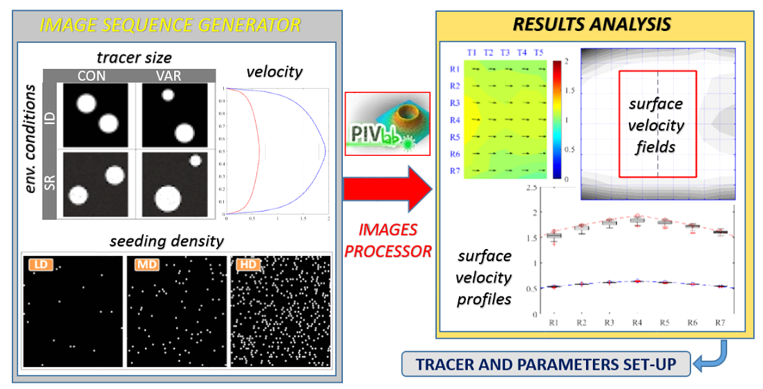
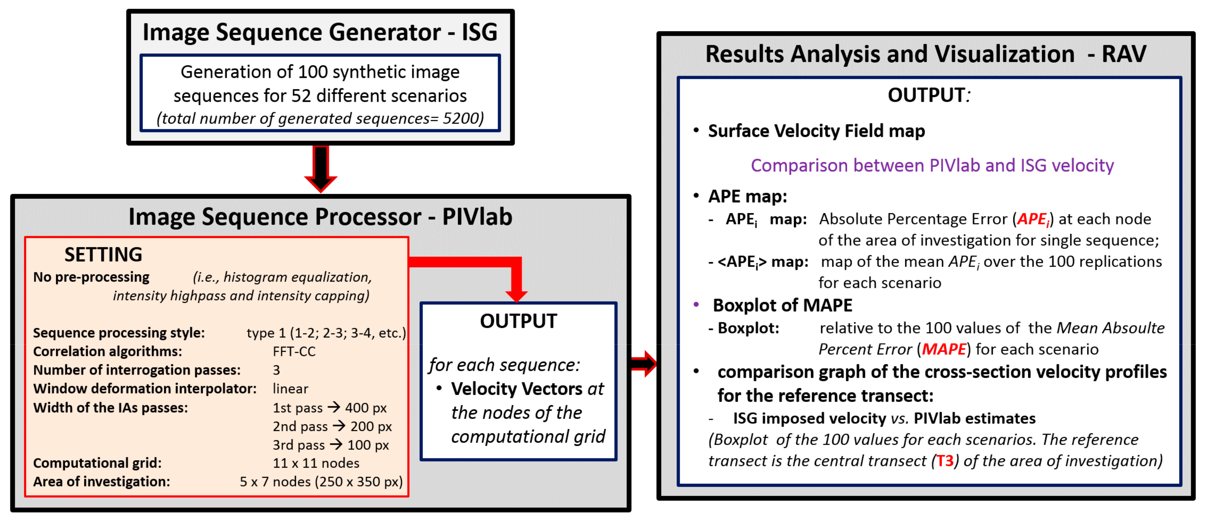
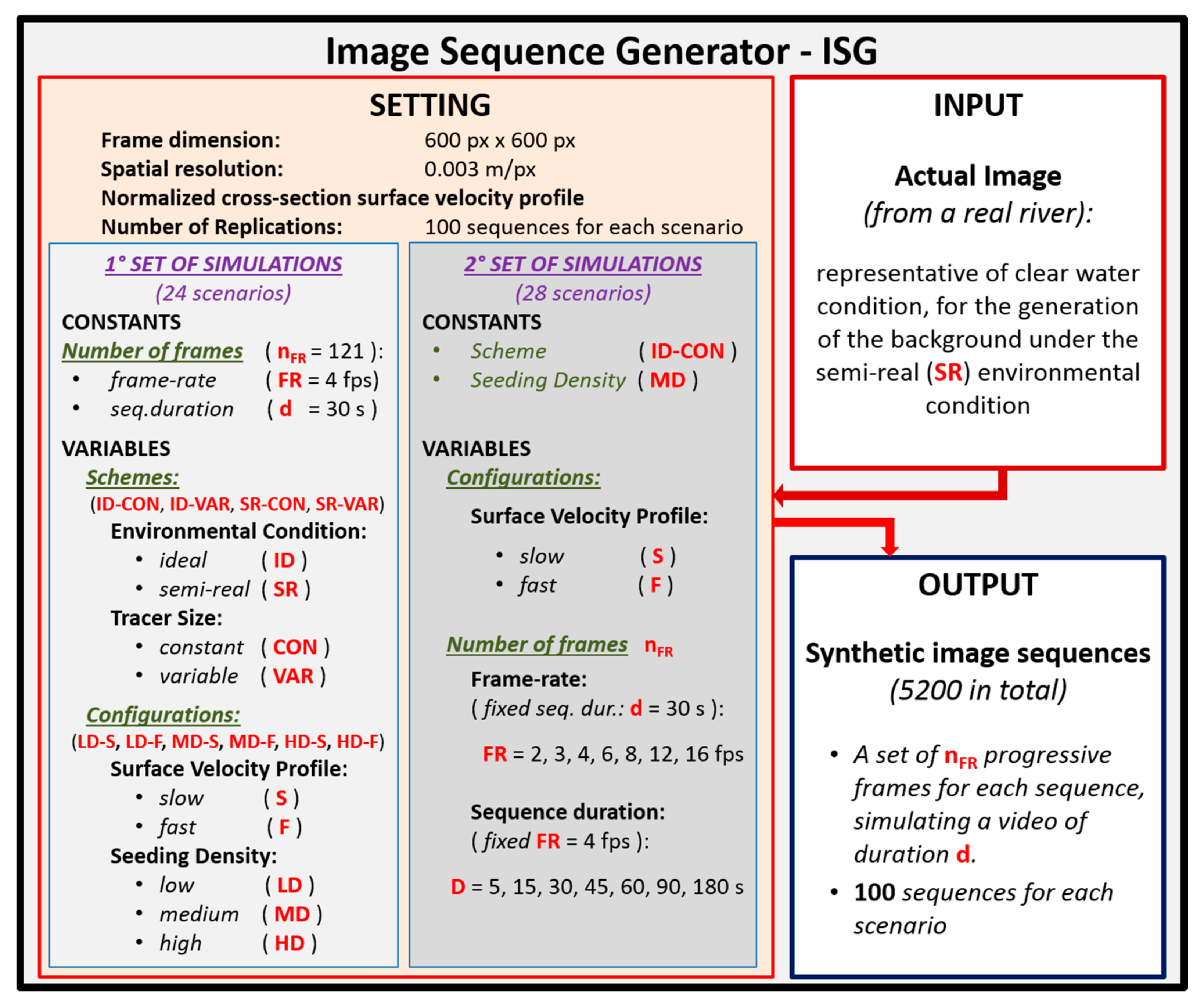
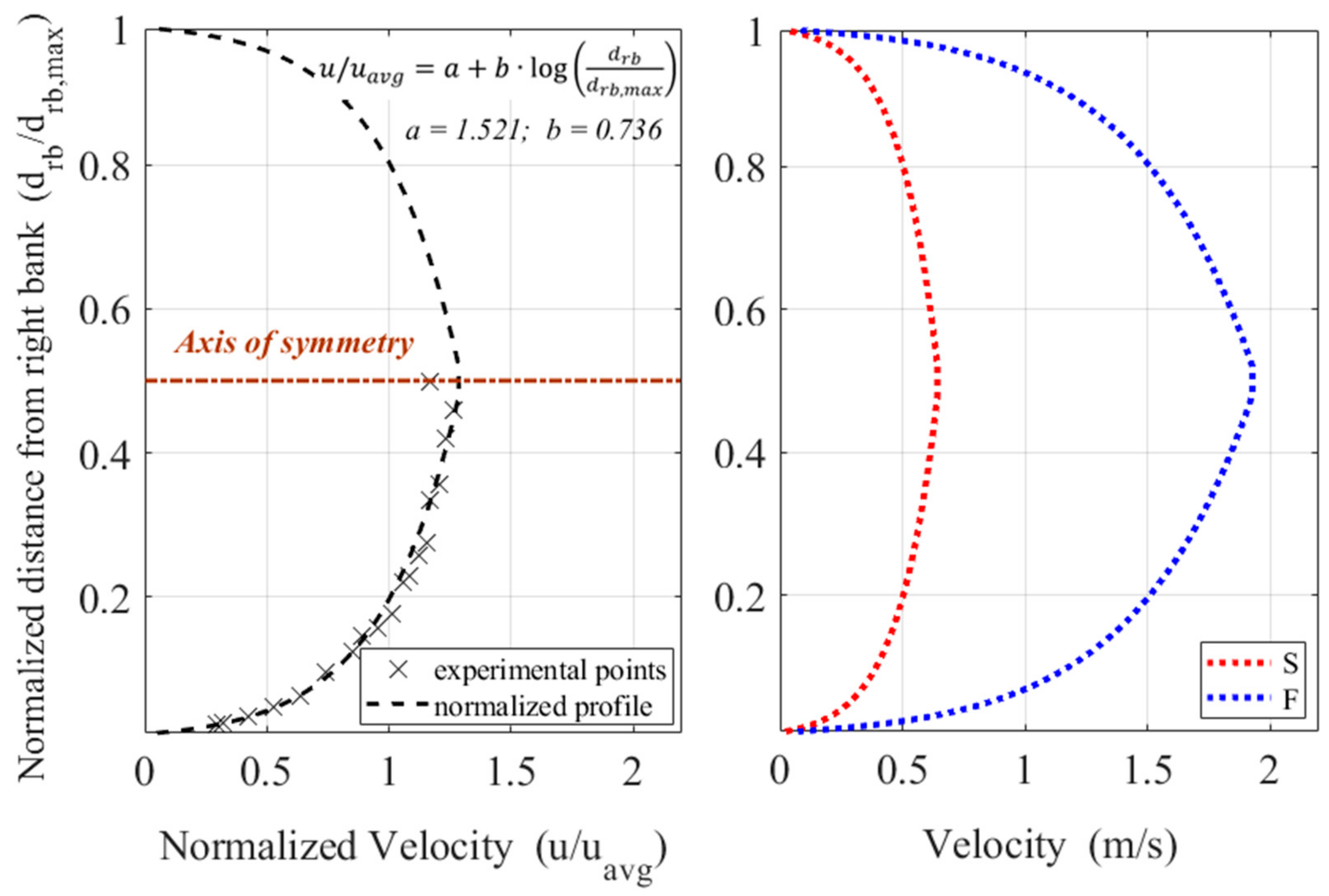
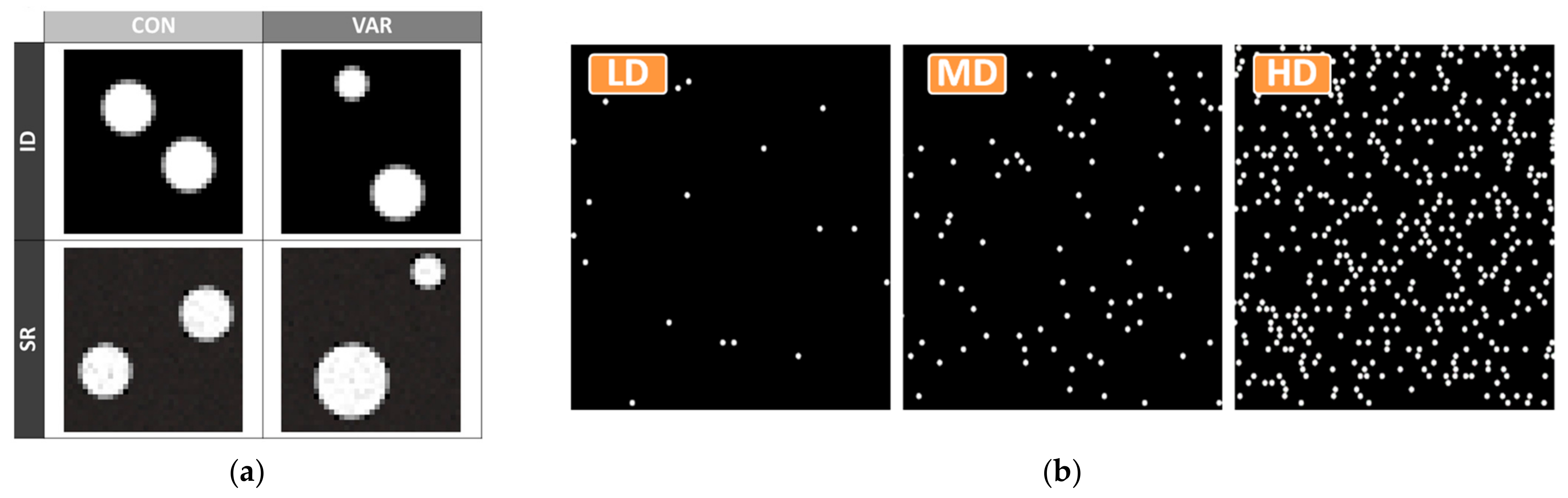
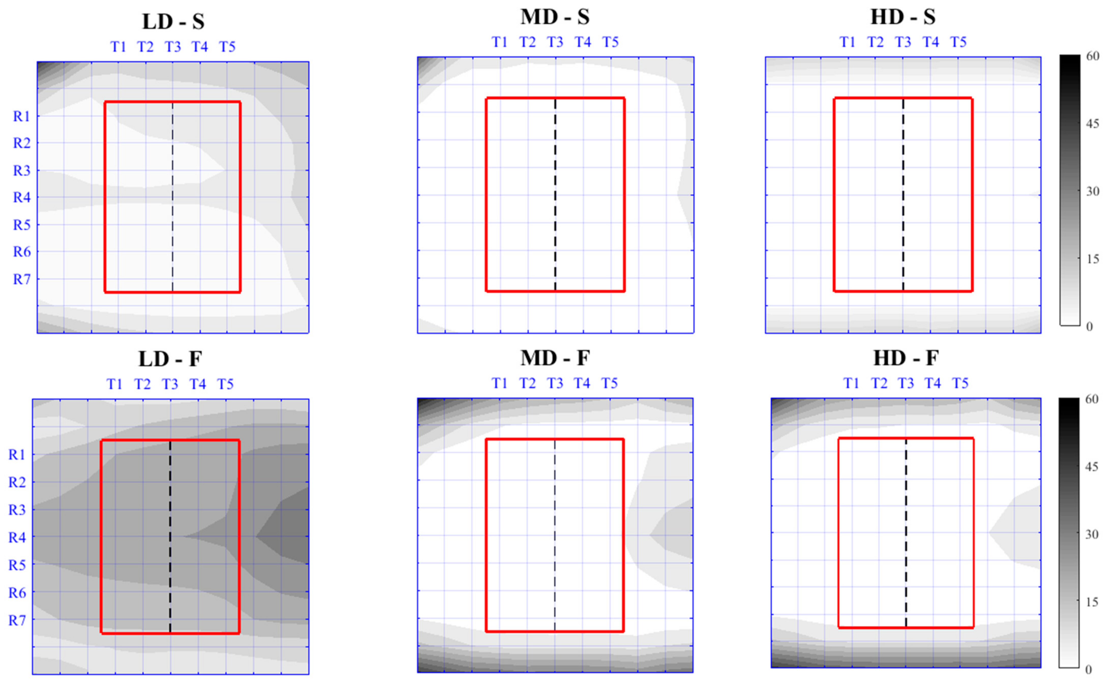
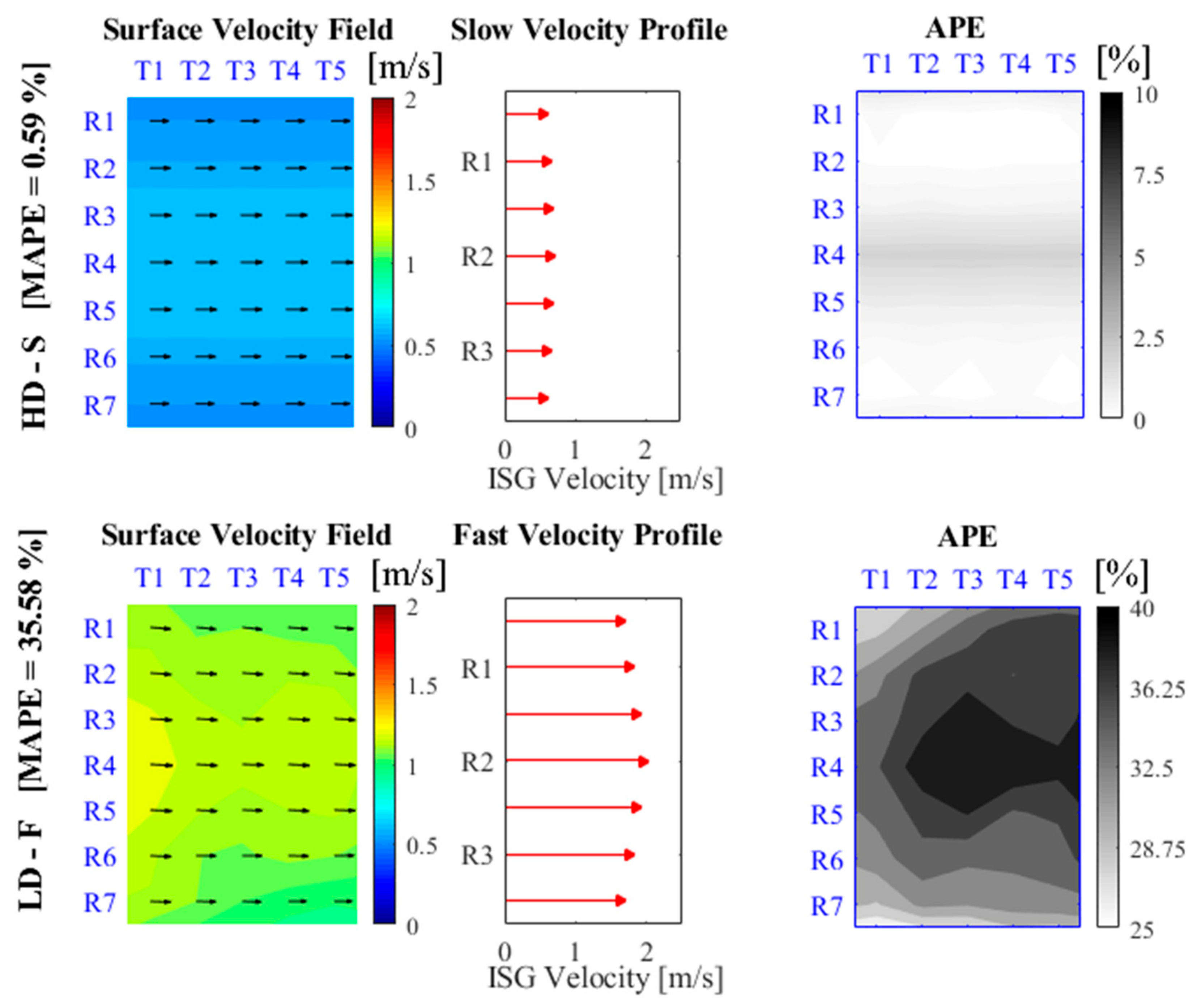
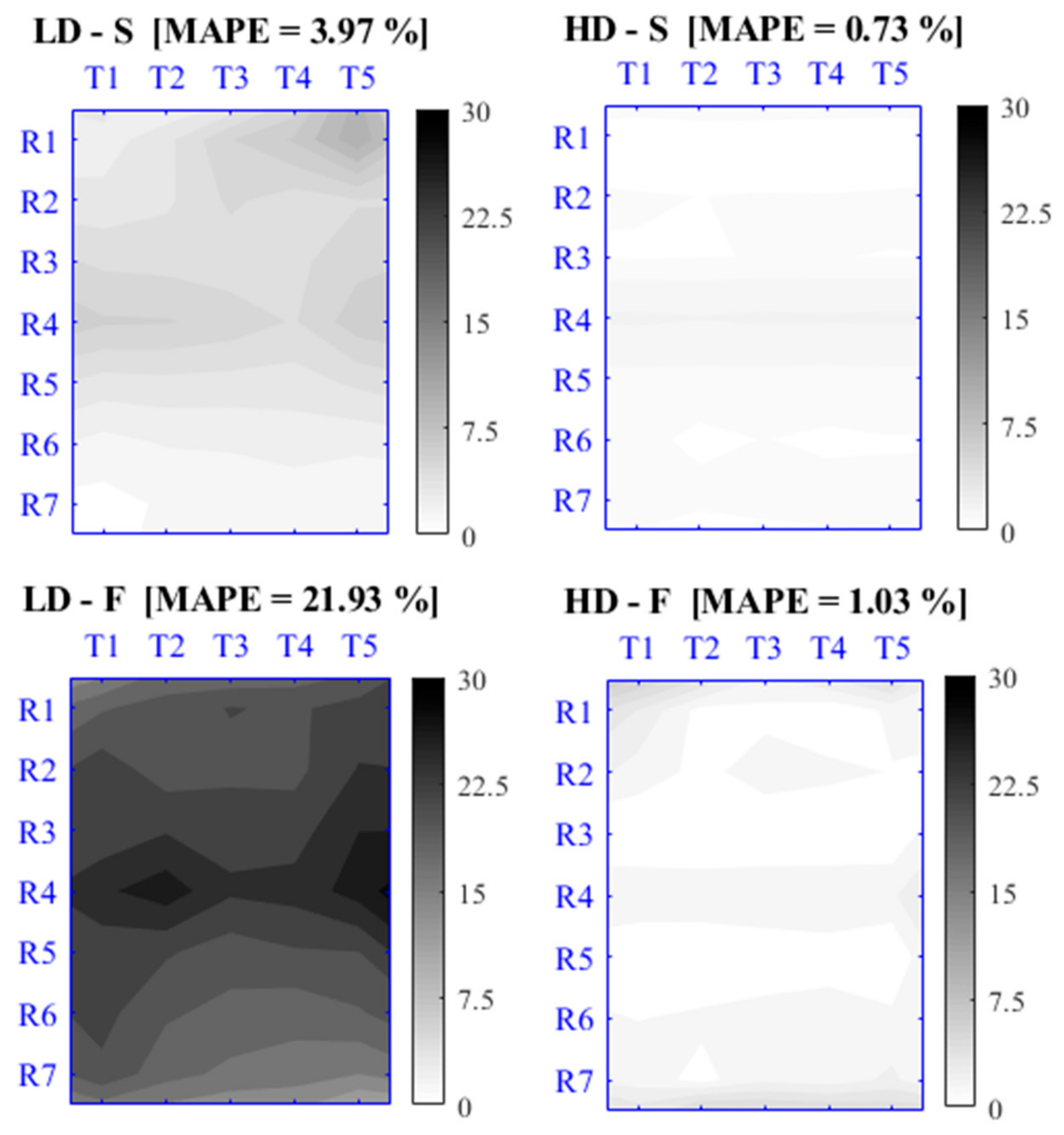
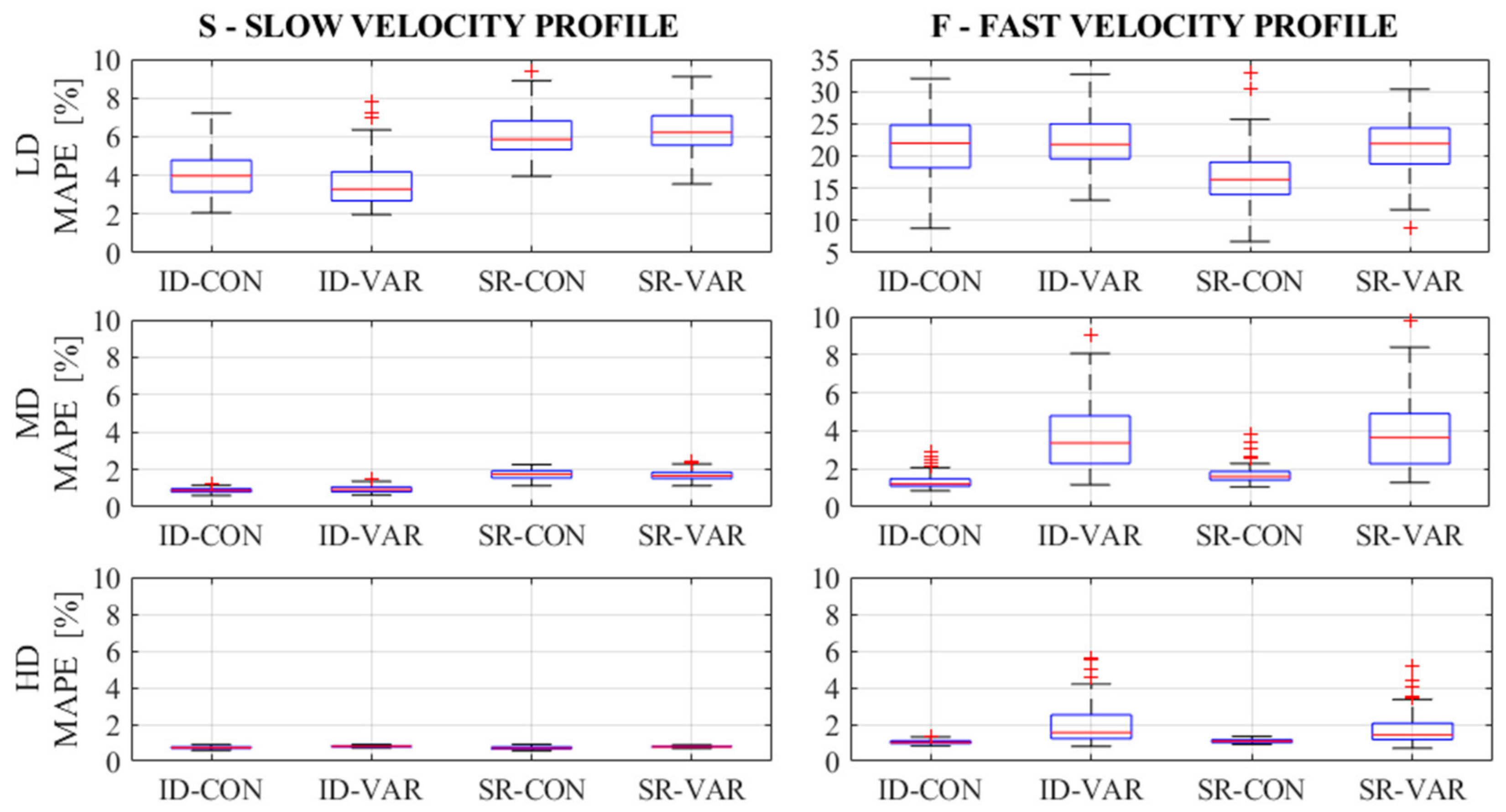
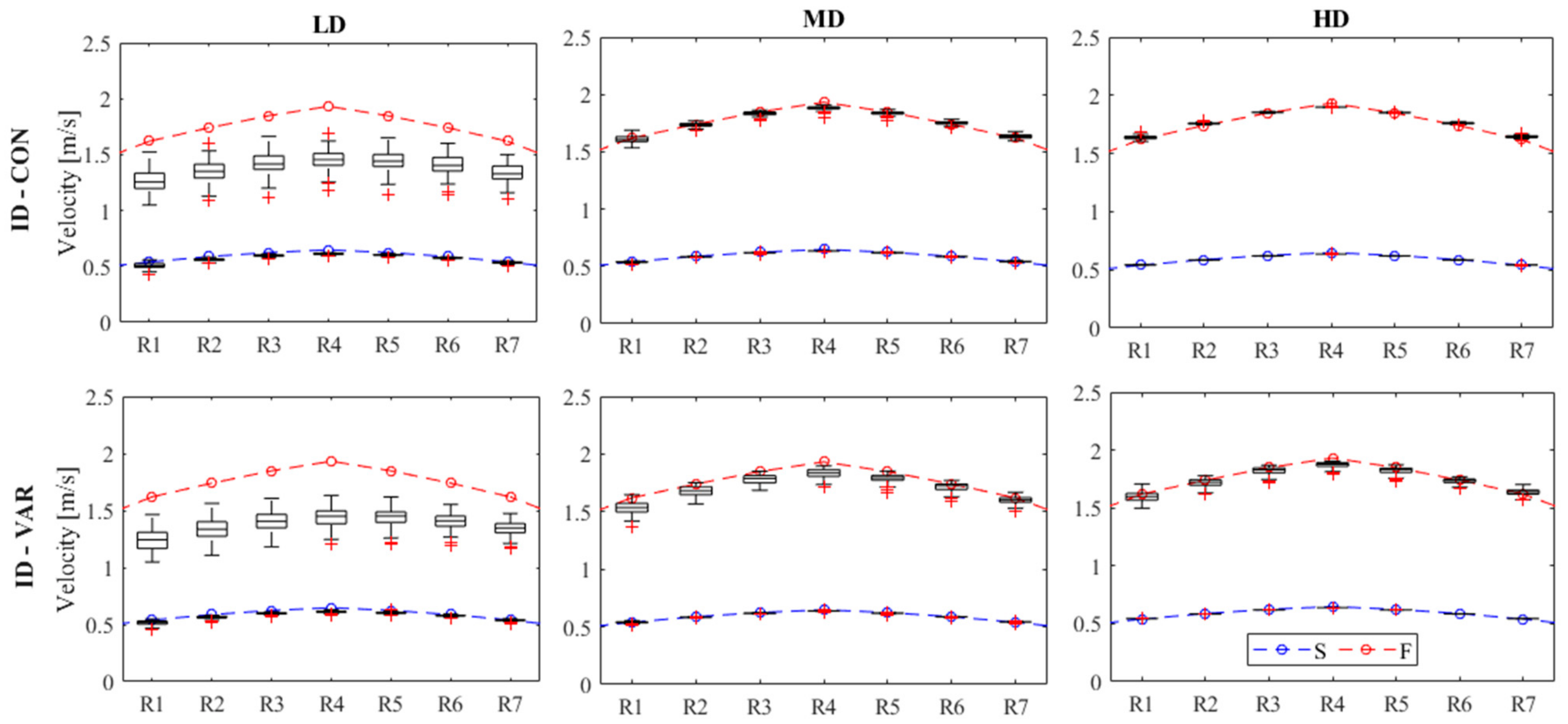
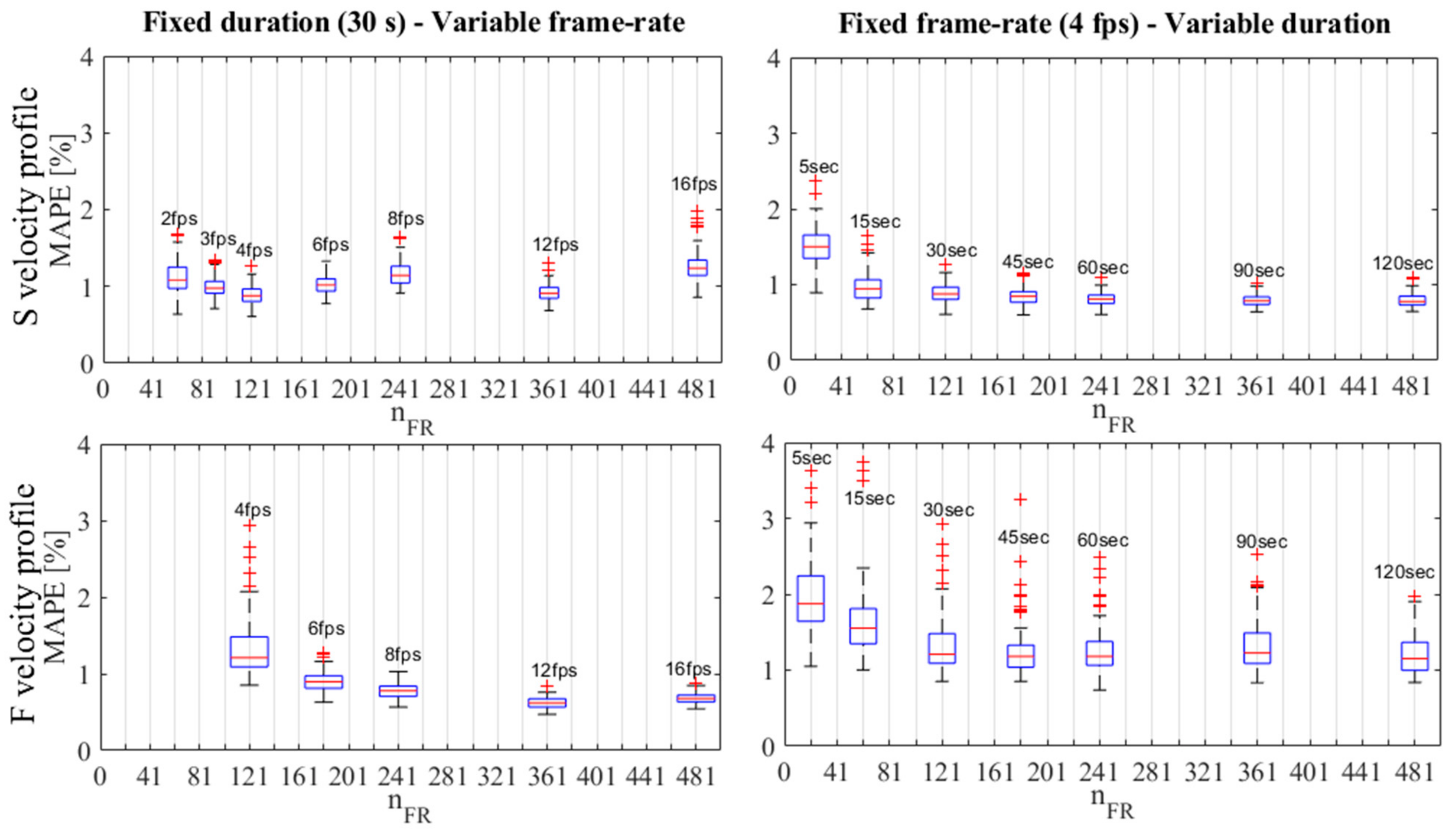
Table 1.
Parameters and configurations considered for generating the 52 different scenarios. The schematic representation in the bottom refers to the different scenarios considered in the first (1) and the second (2) set of simulations. The scenarios are obtained combining schemes (combination of environmental and tracer size conditions) and configurations (combination of seeding density and surface velocity profile). WN = white noise; px = pixel; ppp = particles per pixel; fps = frame per second.
| ENVIRONMENTAL CONDITION | Ideal | ID | Particles Color | white uniform | |||
| Background Color | black uniform | ||||||
| Semi-Real | SR | Particles Color | white unif. + WN | ||||
| Background Color | real clear water | ||||||
| FLOW VELOCITY PROFILE | Slow | S | Average Cross-Section Velocity | uavg | (m/s) | 0.5 | |
| Fast | F | Average Cross-Section Velocity | uavg | (m/s) | 1.5 | ||
| TRACER SIZE | Constant Size | CON | Diameter | D | (px) | 10 | |
| Variable Size | VAR | Mean Diameter | D | (px) | 10 | ||
| St.Dev. Diameter | SD | (px) | 3 | ||||
| SEEDING DENSITY | Low Density | LD | Average Density | λ | (ppp) | 6.4 × 10⁻⁵ | |
| Medium Density | MD | Average Density | λ | (ppp) | 2.5 × 10⁻⁴ | ||
| High Density | HD | Average Density | λ | (ppp) | 1.3 × 10⁻³ | ||
| NUMBER OF PROCESSED FRAMES | Frist set of simulations | Frame-Rate | FR | (fps) | 4 | ||
| Duration | d | (s) | 30 | ||||
| Second set of simulations | Fixed Sequence Duration (30 s) | Frame-Rate Range | FR | (fps) | 2–16 | ||
| Fixed Frame Rate (4 fps) | Duration Range | d | (s) | 5–180 | |||
| PARAMETRIC SCENARIOS | SCHEME | CONFIGURATION | |||||
| LD-S | LD-F | MD-S | MD-F | HD-S | HD-F | ||
| ID-CON | 1 | 1 | 1, 2 | 1, 2 | 1 | 1 | |
| ID-VAR | 1 | 1 | 1 | 1 | 1 | 1 | |
| SR-CON | 1 | 1 | 1 | 1 | 1 | 1 | |
| SR-VAR | 1 | 1 | 1 | 1 | 1 | 1 | |
Table 2.
Frame-rate (FR), sequence duration (d) and total number of processed frames (nFR) for each scenario of the second set of simulations. The corresponding mean frame-by-frame tracer displacement (fr-by-fr displacement) with the imposed velocity profile for both slow (S) and fast (F) velocity case is also reported. The configuration with FR = 4 fps and d = 30 s (highlighted in grey) is common for both first analysis, with fixed duration and variable frame-rate, and second, with fixed frame-rate and variable duration, and it also that considered for the first set of simulations.
| FR | d | nFR | Fr-By-Fr Displacement | |
|---|---|---|---|---|
| slow | fast | |||
| fps | s | frames | px | px |
| 2 | 30 | 61 | 83.3 | 250.0 |
| 3 | 30 | 91 | 55.6 | 166.7 |
| 6 | 30 | 181 | 27.8 | 83.3 |
| 8 | 30 | 241 | 20.8 | 62.5 |
| 12 | 30 | 361 | 13.9 | 41.7 |
| 16 | 30 | 481 | 10.4 | 31.3 |
| 4 | 30 | 121 | 41.7 | 125.0 |
| 4 | 5 | 21 | 41.7 | 125.0 |
| 4 | 15 | 61 | 41.7 | 125.0 |
| 4 | 45 | 181 | 41.7 | 125.0 |
| 4 | 60 | 241 | 41.7 | 125.0 |
| 4 | 90 | 361 | 41.7 | 125.0 |
| 4 | 120 | 481 | 41.7 | 125.0 |
Table 3.
Analysis with fixed frame-rate FR (4 and 12 fps) and variable sequence duration d (30, 45, 60, 90 and 120 s) for the ID-CON (ideal and constant size) scheme and the LD-F (low density and fast velocity case) configuration. For each case, the number of elaborated frames (nFR), the median MAPE and the IQR (in italic) are reported.
| Duration | Frame-Rate (FR) | |||||
|---|---|---|---|---|---|---|
| s | 4 fps | 12 fps | ||||
| d | nFR | Median | IQR | nFR | Median | IQR |
| 30 | 121 | 21.9% | 1.89% | 361 | 3.85% | 1.13% |
| 45 | 181 | 22.0% | 1.58% | 541 | 3.63% | 0.69% |
| 60 | 241 | 21.5% | 1.72% | 721 | 3.51% | 0.64% |
| 90 | 361 | 21.2% | 0.78% | 1081 | 3.50% | 0.29% |
| 120 | 481 | 21.2% | 0.97% | 1441 | 3.48% | 0.19% |
Publisher’s Note: MDPI stays neutral with regard to jurisdictional claims in published maps and institutional affiliations. |
© 2021 by the authors. Licensee MDPI, Basel, Switzerland. This article is an open access article distributed under the terms and conditions of the Creative Commons Attribution (CC BY) license (http://creativecommons.org/licenses/by/4.0/).
Share and Cite
MDPI and ACS Style
Pumo, D.; Alongi, F.; Ciraolo, G.; Noto, L.V. Optical Methods for River Monitoring: A Simulation-Based Approach to Explore Optimal Experimental Setup for LSPIV. Water 2021, 13, 247. https://doi.org/10.3390/w13030247
AMA Style
Pumo D, Alongi F, Ciraolo G, Noto LV. Optical Methods for River Monitoring: A Simulation-Based Approach to Explore Optimal Experimental Setup for LSPIV. Water. 2021; 13(3):247. https://doi.org/10.3390/w13030247
Chicago/Turabian StylePumo, Dario, Francesco Alongi, Giuseppe Ciraolo, and Leonardo V. Noto. 2021. "Optical Methods for River Monitoring: A Simulation-Based Approach to Explore Optimal Experimental Setup for LSPIV" Water 13, no. 3: 247. https://doi.org/10.3390/w13030247
Note that from the first issue of 2016, this journal uses article numbers instead of page numbers. See further details here.