Relationships of Hydrological Seasons in Rivers and Groundwaters in Selected Catchments in Poland


1
Department of Hydrology and Water Management, Institute of Climatology and Hydrology, Faculty of Geographical Sciences, University of Łódź, 88 Narutowicza Str., 90-139 Łódź, Poland
2
Department of Hydrology and Water Management, Faculty of Geographical and Geological Sciences, Adam Mickiewicz University, 10 Krygowskiego Str., 61-680 Poznań, Poland
*
Author to whom correspondence should be addressed.
Water 2021, 13(3), 250; https://doi.org/10.3390/w13030250
Submission received: 17 December 2020
/
Revised: 14 January 2021
/
Accepted: 18 January 2021
/
Published: 20 January 2021
(This article belongs to the Special Issue Climate Change and Human Impact on Freshwater Water Resources: Rivers and Lakes)
Abstract
:The study applied the method of hydrological season identification in a time series of river total and base flows and in groundwater levels. The analysis covered a series of daily measurements from the period 2008–2017 in nine catchments located in different geographical regions of Poland. The basis of the classification of hydrological seasons, previously applied for river discharges only, was the transformation of the original variables into a series reflecting three statistical features estimated for single-name days of a year from a multiyear: average value, variation coefficient, and autocorrelation coefficient. New variables were standardized and after hierarchical clustering, every day of a year had a defined type, valorizing three features which refer to quantity, variability, and the stochastic nature of total and base river flow as well as groundwater stage. Finally, sequences of days were grouped into basic (homogenous) seasons of different types and transitional seasons including mixed types of days. Analysis indicated determinants of types, length, and frequency of identified hydrological seasons especially related to river regime, hydrogeological and hydrometeorological conditions as well as physiographical background were directly influenced by geographical location. Analysis of the co-occurrence of the same types of hydrological seasons allowed, in some catchments, periods of synchronic alimentation (groundwater and base flow, mainly in the cold half-year) and water shortages (all three components, mainly in the warm half-year) to be identified.
1. Introduction
River discharge and groundwater stage are characterized by seasonal variability which is determined by the cyclic changeability of precipitation and evapotranspiration during a year. The multiannual and seasonal variability of flow determinants results in wet or dry years (very often sequences of years) as well as wet or dry summers, etc. [1,2,3]. As a result, during a year, more predictable periods of particular flow phases occurrence appear (e.g., summer floods, autumn low-flows, spring snowmelt). Identification of such periods in a catchment allows hydrological seasons to be defined.
Progress in terms of methodology, quality, and availability of hydrometrical data produces a huge set of measures and procedures used to describe the seasonality of river flows. This set is constantly enriched with new proposals. Very common parameters, widely applied to various components of the hydrological cycle, refer to seasonality index and seasonal time of concentration [4], seasonality coefficient [5], or central of mass data [6]. However, it is rare to find an attempt of numerical identification of sequences of days with similar features of river flow. Only a few analyses have already been made, e.g., [7,8].
They differ in their approaches to flow characteristic estimation. If we make an assumption that river discharge is a stationary, stochastic process, further investigation may be realized in two ways. The first assumes that there is one realization of the flow process only, where a pentad unit in a time structure is applied [9,10]. In the second approach it is assumed that there are many such realizations, for example 365 single-name days from the multiyear [11]. This second approach is relatively new and will be used in the study. In this method, the obtained results are promising because currently the seasonal structure of river flows and groundwater stages is significantly modified by anthropogenic impact, especially water management. Application of statistical methods might help to identify systematic components in time series which indicate some determinants of seasonal structure of water circulation as well as possible level of anthropogenic impact [12]. Therefore, a procedure for the delimitation of specific periods should help to delineate such changes in the hydrological regime. It is worth nothing that for the first time this procedure will be applied to delimitate such periods in groundwater stages.
The aim of this study is to apply the procedure of hydrological seasons identification in relation to total and base river flow as well as the groundwater stage in selected catchments in Poland. No information on the delimitation of seasons concerning base flow and groundwater stages is found in the literature, and the authors believe that it has not yet been attempted. Therefore, analysis of the co-occurrence of the same types of hydrological seasons in all three components and its determinants is the second main aim of this work.
2. Materials and Methods
2.1. Study Area
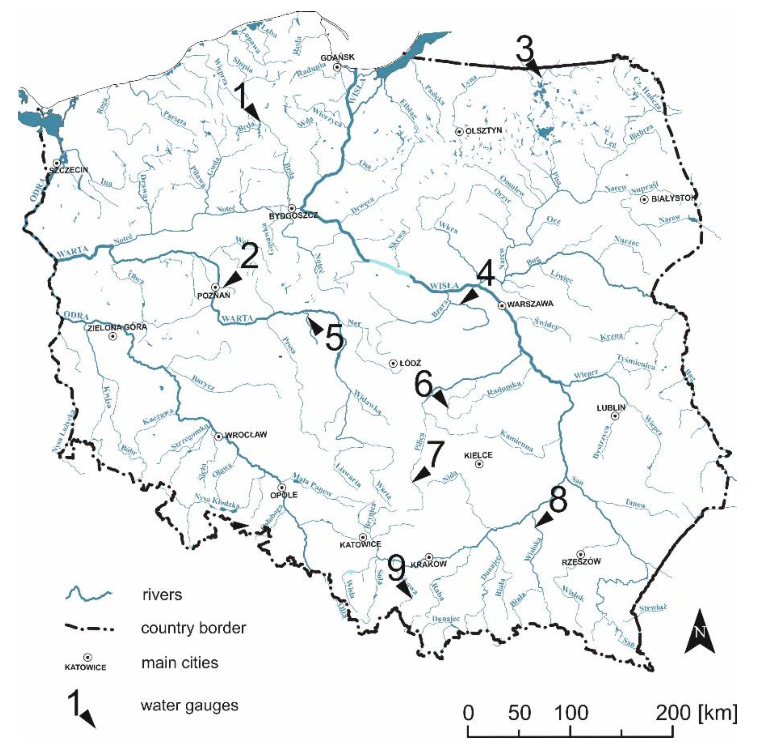
The basic hydrometrical material used for this research was derived from nine water-gauge stations serviced by the Polish Institute of Meteorology and Water Management—National Research Institute. Catchment areas closed by these water gauges were not significantly differentiated; from 140 up to 1200 km2 (Table 1). When choosing the catchments for the study, the authors endeavored to make a selection that would represent various climatic and physiographic conditions, above all, one in which the rivers would reflect different types of hydrological regime. Among the analyzed gauges, three cross-sections were located on lake district rivers, two on lowland, two on upland, and two on mountainous streams (Figure 1). Such selection allows to analyze different river regime behaviors, especially in matter of flow dynamics and retention determinants. For example, in a mountainous catchment, high flow variability and significant precipitation alimentation are expected, in a lake catchment flow smoothing and the lake basin retention capacity plays important role in hydrological regime whereas a lowland catchment will be prone to development of severe hydrological droughts. As a result, the chosen sample of catchments reflects a wide spectrum of types of hydrological seasons which are possible to be identified. The presented catchments are small or medium in size which guarantees relative homogeneity of water circulation determinants. It should be also noted that they are placed far from big urban and industry zones, and water management objects and activities within them do not have a significant impact on surface and groundwaters.
Within each catchment one groundwater station, serviced by the Polish Geological Institute—National Research Institute, sampling groundwater level at daily intervals was selected. The chosen stations were located as closely as possible to a river water gauge station, and where the measured groundwater table was drained by river channels (Table 1). All investigated aquifers are unconfined. The main alimentation process is infiltration of precipitation which shapes water table placed on average between 0.6 and 7.8 m below surface. In most cases aquifers are of the Quaternary origin and are made of sands and gravels which guarantee good filtration. Only upland aquifers originate from the Triassic and Cretaceous periods. They have good retention conditions as well because they collect groundwaters in well fissured marls and sandstones. All sampled groundwater reservoirs are drained by river channels with good hydraulic contact. The phreatic and topographic watershed divides run one above the other. As a result, groundwater alimentation is restricted to surface catchment area only. Therefore, they are not large and reflect processes taking place within the river basin, especially the time of reaction of groundwater table to rainfall alimentation in relation to the base flow behavior. The local range of aquifers as well as lack of urban and industrial zones make them free of hydro-political issues or significant degradation problems which are characteristic of large, transboundary groundwater reservoirs [13,14].
2.2. Data Set
The input data consisted of a daily series of river discharge and groundwater levels from the observation period of 2008–2017. The analyzed multiyear period guarantees the occurrence of seasons with various moisture conditions and various structures of the water balance, and thus the appearance of such hydrological extremes as droughts and floods of various severity, extent, and duration. The obtained results were presented in the convention of a hydrological year, which in Poland and some other countries starts on 1st of November and terminates on 31st of October.
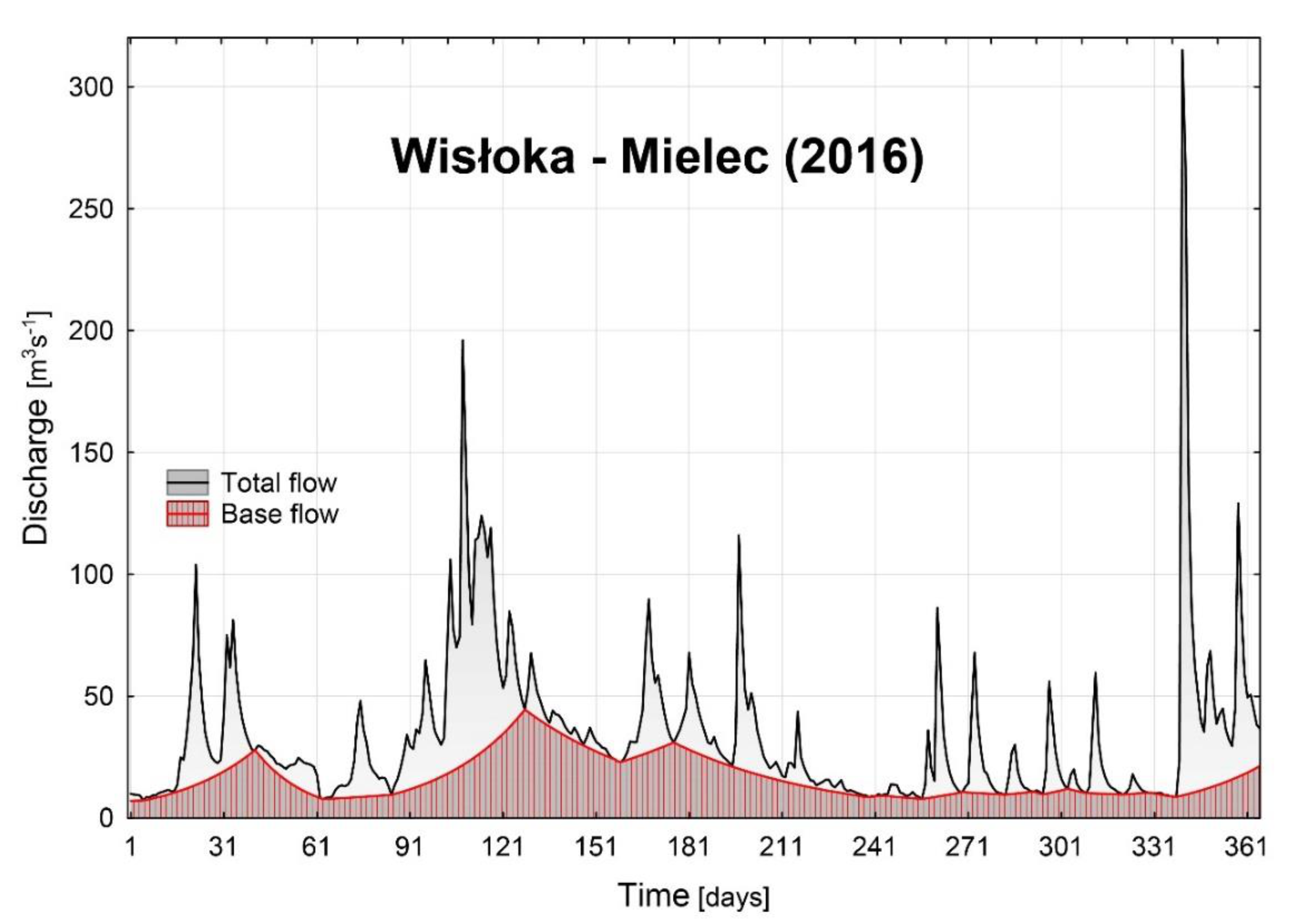
During river flow regime analysis, the base flow component was separated. It reflects the quantity and intensity of river channel alimentation by groundwaters. Its analysis allows an assessment to be made of the dynamics of aquifers which are in hydraulic connection with river channels. Estimation of the base flow component was based on an automatic separation algorithm proposed by Tomaszewski [15]. This idea develops the simple numerical methods which date from at the early 1990s [16,17] and is based on daily discharge values only. Thanks to an analysis of recession curves transformed into a natural logarithmic scale and an assumption that the daily groundwater flow rise gradient cannot be higher than the modulus of mean daily discharge recession gradient, effective smooth exponential curves dividing the total river discharge into base and quick flow components on the flow hydrograph were drawn (Figure 2). As a result, a daily series of total flow and an estimated series of base flows were taken for further research.
2.3. Statistical Analysis
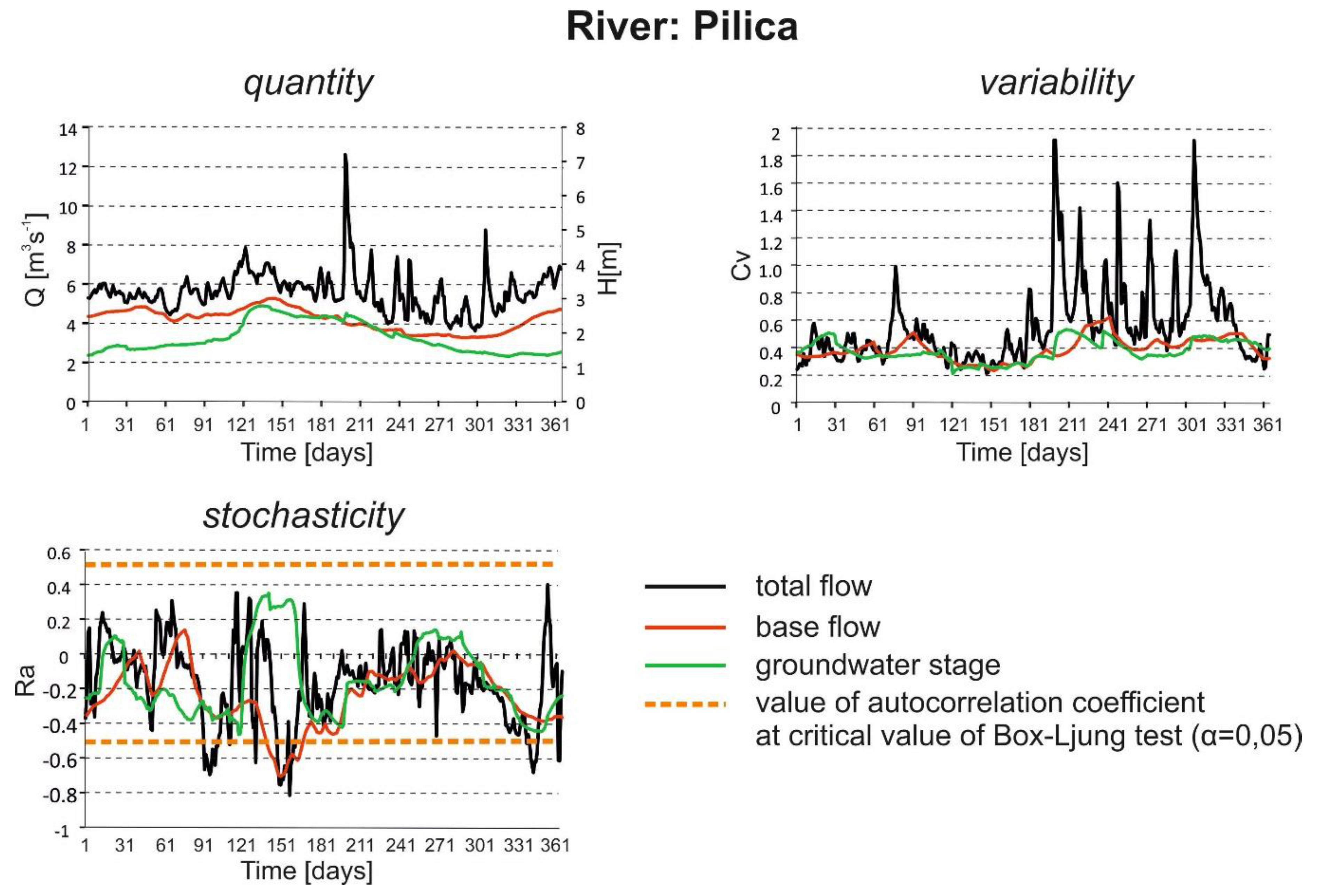
The assessment of the seasonal nature of the hydrological regime in was based on three main statistical characteristics which refer to such features of the investigated processes as quantity, variability, and stochasticity. For this purpose, a series of daily total flows, base flows, and groundwater levels for each set of components were used in further transformations. Based on these characteristics for each catchment new time series were created with 365 elements of mean multiannual total and base flows for each single-name day of a year (TF, BF) as well as for groundwater stages (GS). The next step of the procedure was to calculate a multiannual variation coefficient for each day of a year for all three parameters: CvTF, CvBF, CvGS. The final transformation was a calculation of an autocorrelation coefficient with a lag equal to 1 (which is equal to 1 year in this case, for example: 1.XI.2008-1.XI.2009-1.XI.2010 etc.) for each single-name day all of the three variables: RaTF, RaBF, RaGS. Statistical significance of the estimated coefficients was verified on the level α = 0.05 on the basis of the Box-Ljung test [18]. Thus, for each catchment nine new 365-day series of quantity, variability, and autocorrelation in a multiyear for total flow, base flow, and groundwater stage were estimated (Figure 3). The variables that were calculated can easily be interpreted physically—the average multiyear TF, BS, or GS on a given single-name day is an estimator of the temporary water quantity in the catchment on that day. The variation coefficient (CvTS, CvBS, CvGS) reflects the long-term variability (or stability) of the catchment’s water resources. An insignificant autocorrelation coefficient (RaTS, RaBS, RaGS) informs about the stochastic distribution of time series, and a significant one—about the existence of long-term inertia or periodicity in total flows, base flow as well as groundwater stages.
2.4. Cluster Analysis
The new variables differed in variances and distributions. Therefore, to satisfy further statistical procedures, they had to be standardized. For this purpose, a simple and very well-known procedure was used [19]:
where xs is standardized variable; xi is original variable; xs is arithmetic average; δ is standard deviation.
Such a transformation ensures that all the variables have a distribution with a mean equal to 0 and a standard deviation equal to 1. This makes it possible to compare them with each other and makes the conducted analysis independent of the units in which the variables were measured [20].
Standardized time series of quantity, variability, and autocorrelation in multiyear for total flow, base flow, and groundwater level were used for definition of types of day. After this procedure, every single-name day of a year was assigned to type of day, described by the three above-mentioned parameters. To define types of days, hierarchical clustering in three-dimensional space (quantity, variability, and autocorrelation coefficient) was carried out separately for TF, BF, and GS characteristics in every catchment. For clustering, the most frequently used Ward’s method was chosen [21,22]. This is a well-known and described procedure, used in hydrological research, including assessment of changes in river regimes [23,24,25,26,27,28]. It should be highlighted that the procedure is very sensitive to differences in the variance of agglomerated data, and the time series with the highest variance have the greatest impact on the identified clusters. To avoid this influence, it is recommended to carry out hierarchical clustering of data with similar variances [21,22]. For this purpose, the standardization procedure on the input data was performed (Equation (1)).
In the hierarchical clustering analysis, accumulation of objects (in this case 365 days) is managed until the creation of one cluster. Therefore, the next step was to choose the correct number of clusters appearing in this procedure. A correct number of clusters guarantees that the delimitated ones are as homogeneous as possible (quantity, variability, and autocorrelation for days collected inside the cluster from a very similar range) and maximally different from other clusters. There are various methods for estimating the correct number of clusters [29,30]. One of them is to evaluate a stopping criterion which indicates at which step further clustering should be stopped (number of clusters in a selected step is optimal and next clustering should be avoided). In the present study, the stopping criterion known as the “Moyena rule” was used [31]. This is one of many stopping criterions characterized by simplicity of calculation and its relative acceptability by researchers in the matter of number of clusters [32]. It is calculated according to the formula:
where Rm is Moyena’s rule; dh is average distance between connecting clusters; δ is standard deviation of distances between connecting clusters; b is equation constant (2.75–3.50).
For samples containing hundreds of elements (in this case 365 days), the maximum possible equation constant value is preferred (which is 3.5), and this parameter was chosen for further analysis. As a result, the procedure of hierarchical clustering should be stopped when the next distance between the accumulating clusters is higher than the calculated value of Rm.
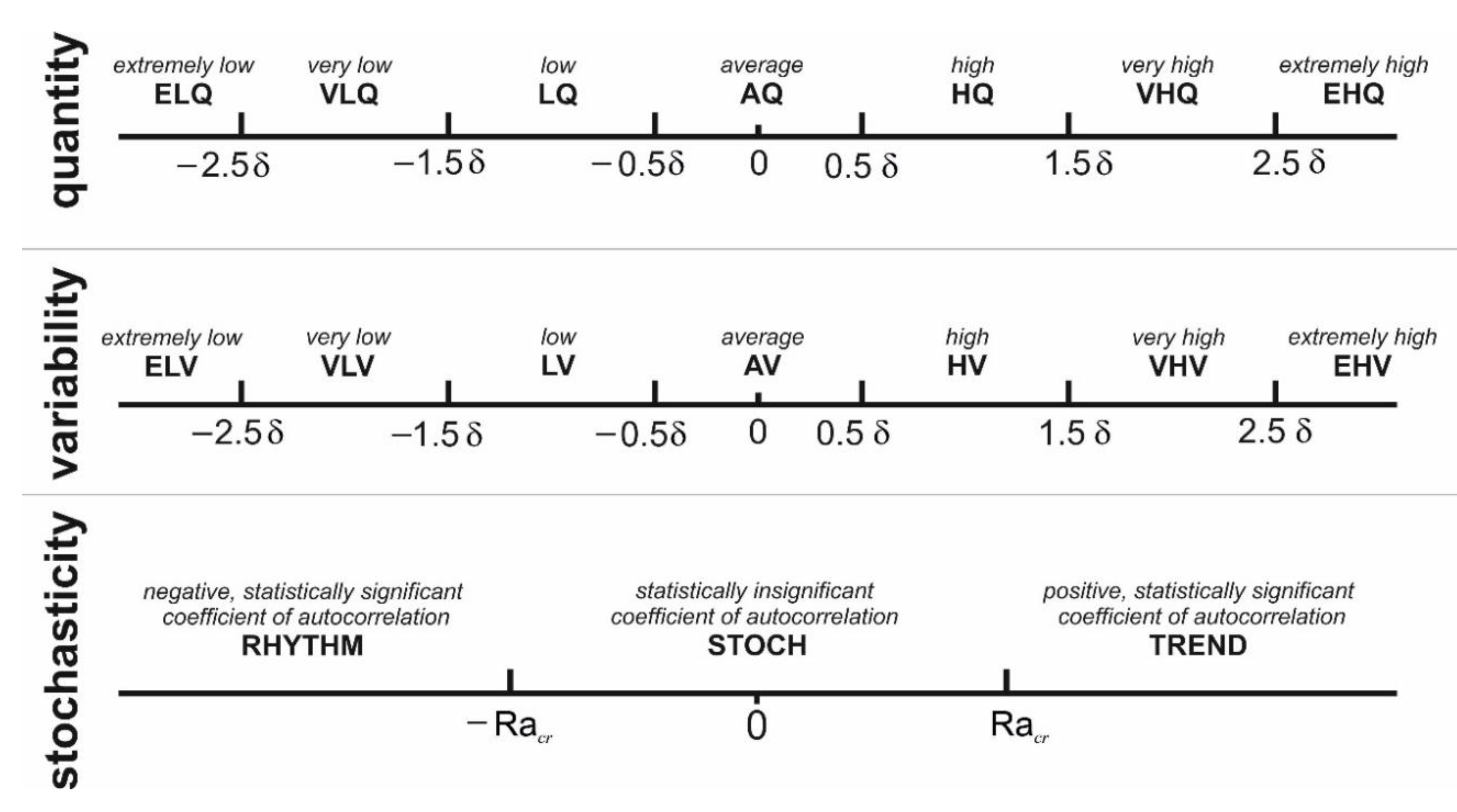
The results of hierarchical clustering allow the types of day in the investigated time series to be identified according to the scheme presented in Figure 4. For vectors describing quantity and variability, the average and standard deviations were calculated. It was then verified whether days with a statistically significant autocorrelation coefficient Ra (separately Ra > 0 and Ra < 0) dominate in each type of day or if this autocorrelation is statistically insignificant. Using calculated averages and standard deviations as well as the significance and sign of autocorrelation coefficients, according to the scheme (Figure 4), hydrologically interpretable names of the identified types of days were proposed.
2.5. Identification of Hydrological Seasons
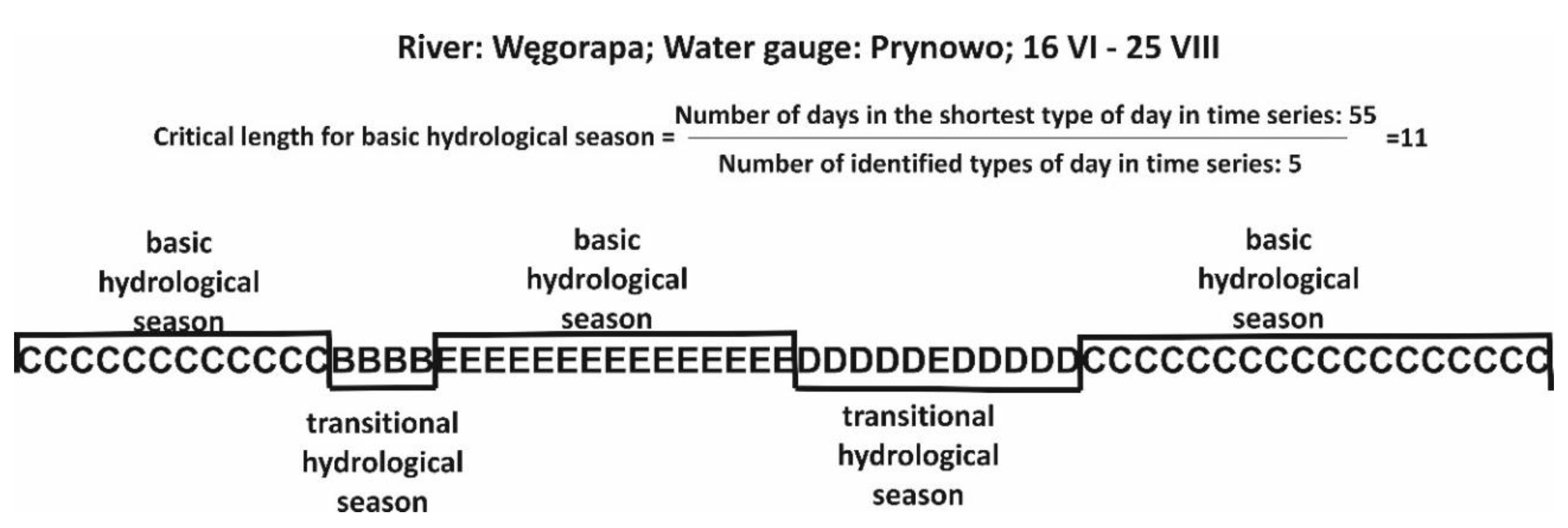
In the last step of the procedure, the delimitation of hydrological seasons in a chronologically ordered time series of single-name days of a year was made. An improved method of delimitation of hydrological seasons was applied. Every examined time series consisted of some sequences representing the same type of day and sequences where types of days were mixed day by day. A sequence of the same type of days might be identified as a basic hydrological season when its length is equal or longer than the critical length. The critical length of sequence, which is a new addition to the procedure with respect to the previous proposition of Jokiel and Tomalski [33], is calculated for every time series separately:
where Crl is critical length for basic hydrological season; Nmin is number of days in the shortest type of day in a time series; N is number of identified types of day in a time series.
Sequences of the same type of days longer or equal to the critical length were identified as basic hydrological seasons. Sequences of the same type of days shorter than the critical length or consisting of a mixed sequence of types of days are defined as transitional hydrological seasons. An example of the delimitation procedure of hydrological seasons is shown in Figure 5. The names of the identified types of basic hydrological seasons are inherited from the types of day existing within them. Transitional seasons do not have names.
3. Results and Discussion
In 27 examined time series (nine catchments and three investigated components) 21 types of day were delimited (Table 2). It is worth noting that in the study published by Jokiel and Tomalski [33], in a group of 25 water gauges located in major Polish rivers (Vistula and Oder), a very similar number of types was identified—22. In the group of investigated catchments there are some types of day which occur very frequently in all three hydrological components—types numbers 8, 12, 16 (Table 2). They are characterized by low or medium variability and a lack of statistically significant autocorrelation in the time series. Types restricted to one catchment and one variable only also appeared (types no. 3, 7, 9, 17, 19, 20, 21).
Two types of day had no representation in basic hydrological seasons (no. 1 and 7 in bold in Table 2). The first was delimited for total flow in two rivers (the Skawica in the mountains and the Pilica in the upland). These types of days represent extremely high flows with extremely high variability without autocorrelation in a time series. Such cases were observed rarely, which verified the low number of days in that group (in both rivers—15 days in total). Moreover, they are associated with high floods, which are typically of short duration in mountain and upland rivers. Therefore, despite the relatively short critical length of the basic hydrological season (Table 3), it was not possible to identify such a season in these rivers.
The second type of day which did not constitute a basic hydrological season was identified in groundwater levels in the aquifer of the Skawica river catchment. This is a shallow aquifer collecting groundwater in quaternary alluvial sands and gravels (Table 1). In such groundwater reservoirs variability of the water table is high, which determines in a chronologically ordered time series significant mixing of types of day. It is difficult to find a long enough period with the same types of days, therefore, transitional hydrological seasons dominate in this case (Table 3).
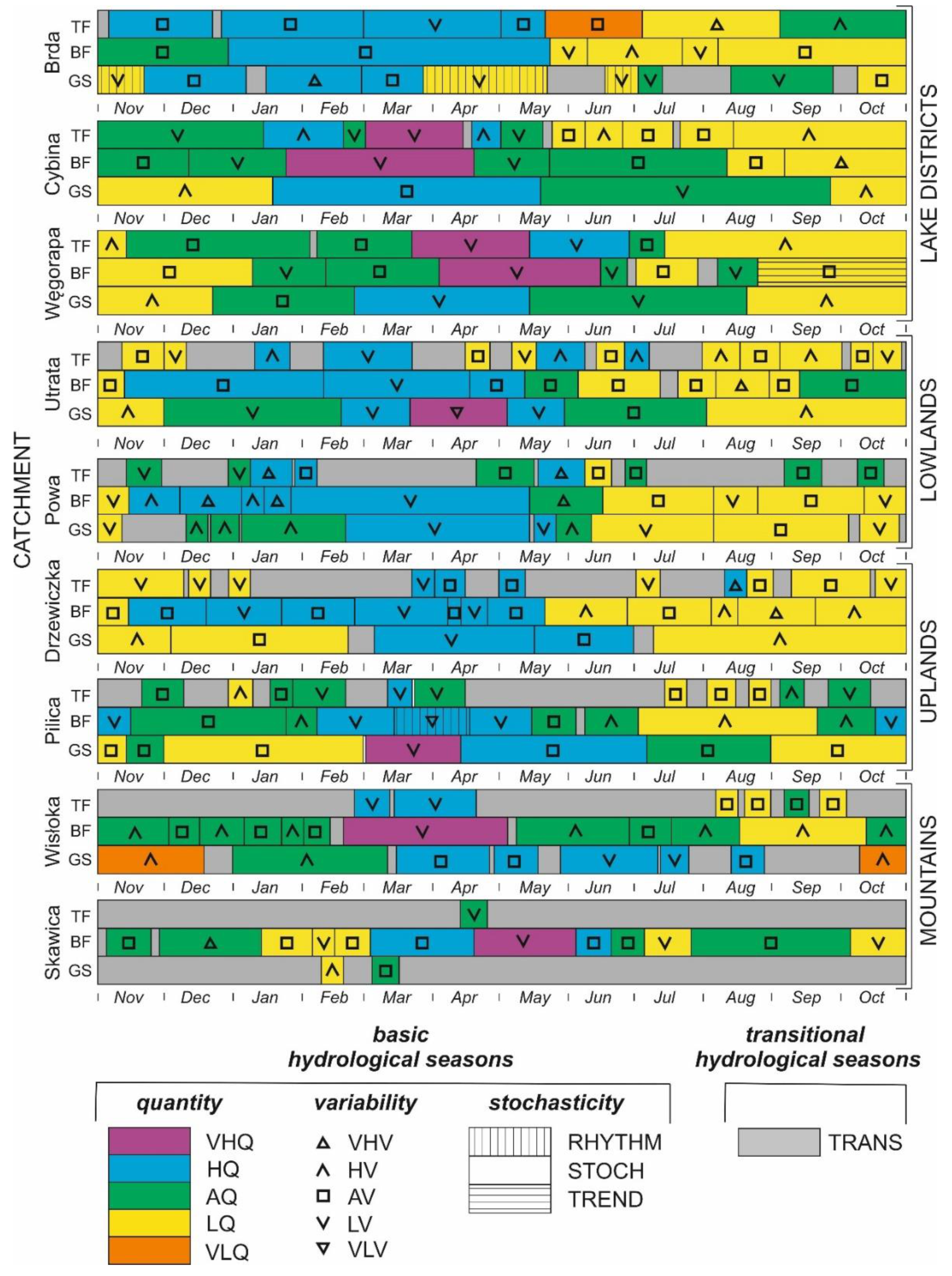
The pattern of identified hydrological seasons for total and base flows as well as groundwater levels during a year in the examined catchments is shown in Figure 6. In some studied time series, one type of basic hydrological season occurred in a selected catchment once, for example basic hydrological season number 6 in the Brda river for base flows (Table 2, Figure 6). In other cases, one type appeared a few times and maximum frequency was observed in the season of type 11 in the Wisłoka river for base flows (six occurrences).
The number of occurrences of hydrological seasons of different types in the selected catchments ranges from three per year (Skawica river for total flows) up to 22 times per year (Utrata and Pilica rivers for total flows). Interestingly, there are no relations between the number of season occurrences and any other characteristics of the studied catchments. Moreover, a large number of occurrences is not reflected in high variability of total flow, base flow, or groundwater stages.
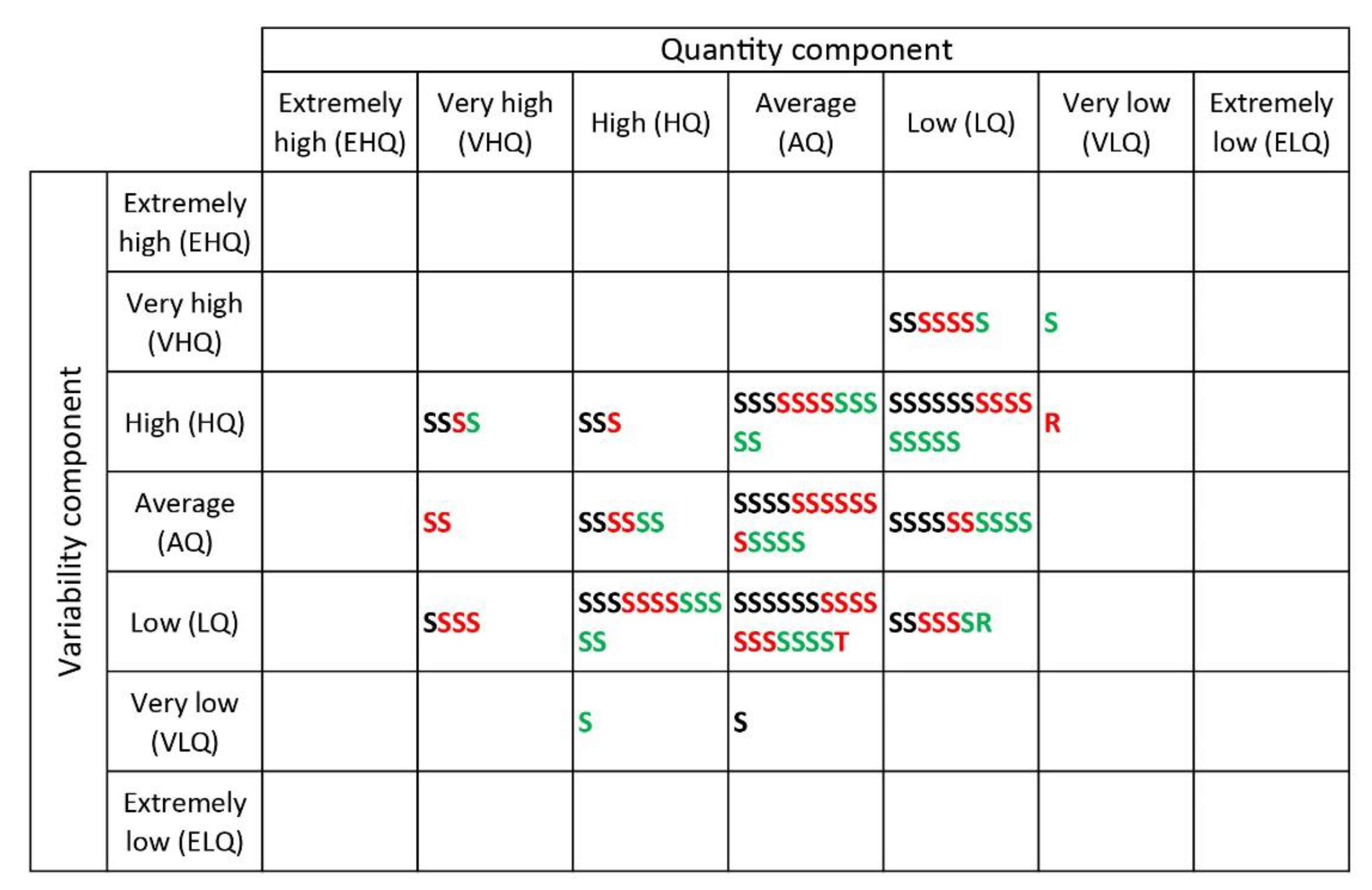
Distribution of the main features of the identified basic hydrological seasons in all three investigated components of water circulation is characterized by a few regularities (Figure 7). Almost all types of season have a stochastic nature in a multiyear scale which means that there were no significant systematic determinants in time series (one case of trend and two cases of rhythm), caused by anthropogenic pressure or serious hydrometeorological fluctuations. As expected, the identified seasons were concentrated near average values of quantity and variability of water resources (Figure 7). There were no seasons with extreme features because there were no sequences of ‘extremal’ days that were long enough. Almost every type of season possessed representatives in all three components. However, very high variability was related mostly to the base flow component, whereas only two cases of very low variability were counted (one base flow and one groundwater stage). A quite similar pattern along the quantity axe was also observed. A very high quantity was dominated by the base flow component while a very low one consisted of two elements only (total flow and groundwater stage).
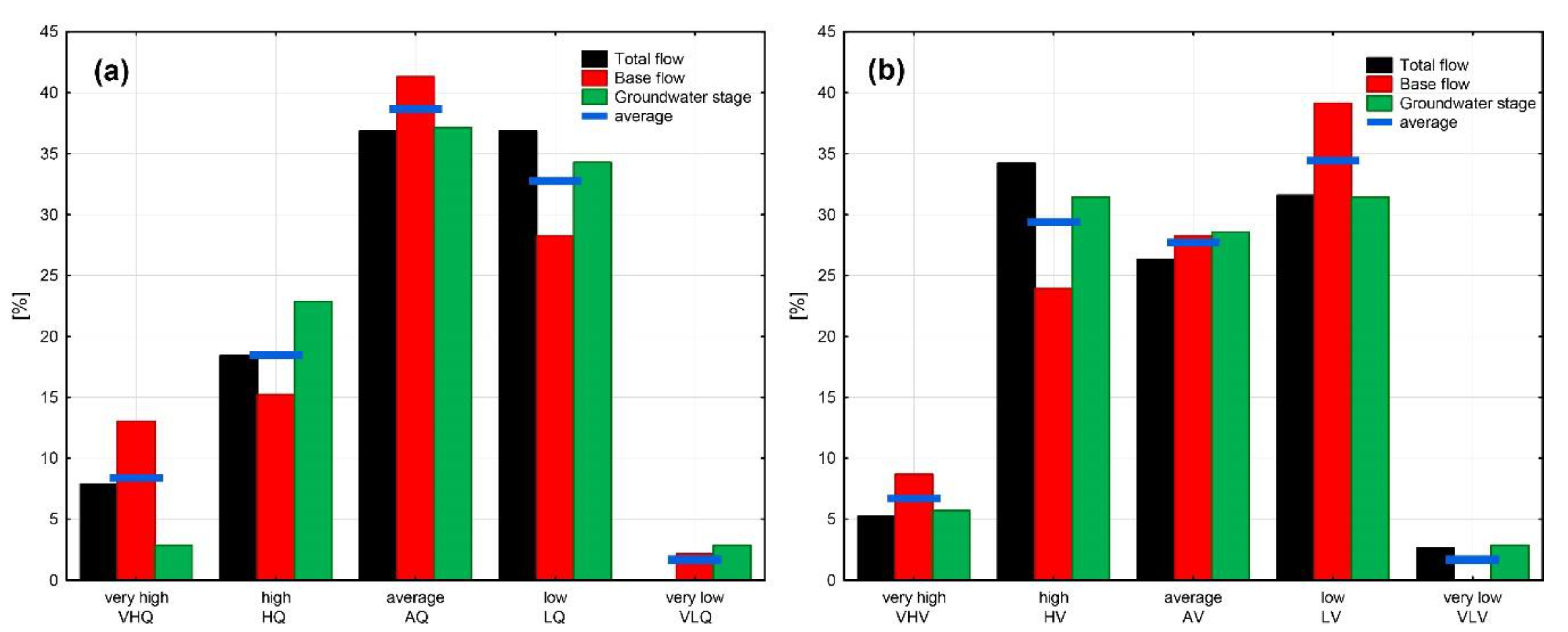
The distribution of identified seasons in quantitative classes was characterized by significant asymmetry (Figure 8a). A clear negative skewness confirmed the question mentioned above where base flow seasons occur above average in very high and mean classes. Total flow is ‘active’ in high and low class, whereas groundwater stage seasons are highly presented in high as well as low and very low classes. Seasonal distribution in variability classes is much more symmetric than the previous one (Figure 8b). Average variability occurs very similarly in all three components. Classes near average do not differ significantly from average, however, the base flow component is more frequent in the low class and less frequent in the high one. Types with higher or lower flow and stage dynamics appear very rarely in hydrological seasons and it is worth noting that there was no base flow season with a very low variability.
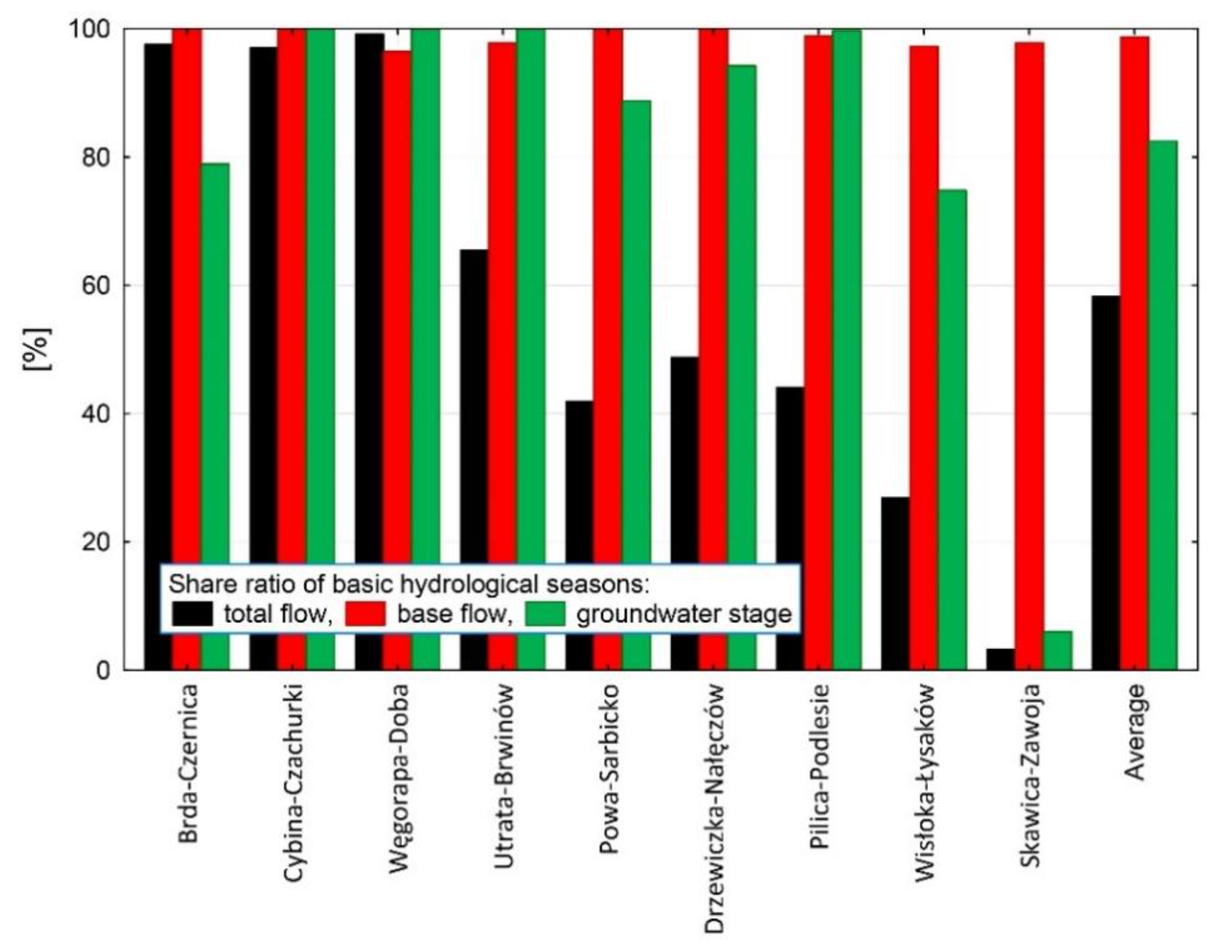
River flow regime, groundwater stage changeability as well as local geographical conditions determine the length and stability of hydrological seasons in the investigated catchments. Quantitative assessment of this problem was made on the basis of the share of the number of days with the basic hydrological season in the number of days in the whole year (Figure 9). On average, basic base flow seasons lasted almost the whole year in every catchment. This is probably determined by very high inertia of groundwater flow drainage by river channels [15,34,35]. It depends on the specific pace of recession and the renewal of groundwater resources and on the level to which reservoirs are filled [36,37]. As a result, chronological base flow changeability is low enough to ensure that all criteria for hydrological season identification are almost always satisfied. Basic seasons of the groundwater stage last more than 80% of a year on average. This is also determined by high inertia of main alimentation process, which is infiltration. It is significantly modified by the geostructural and geofiltrational properties of aquifers as well as the depth of groundwater table occurrence. As a result, the share index of the groundwater stage basic season is slightly lower than the similar index estimated for base flow. The stochastic nature of hydrometeorological conditions, very important in total flow alimentation, makes the basic seasons for this component shorter during a year.
From geographical point of view the longest duration of the basic hydrological season during a year is characteristic of lake district catchments (Brda, Cybina, Węgorapa)—Figure 9. The long duration of the percentage in all three investigated components results from the stabilizing function of the lake basin in the groundwater drainage process and river flow formation. All streams flowing through or out of the lakes have their water resources extended by lake basins. The capacity of the temporarily unfilled volume of lake basins might reduce flood discharges in the catchment. In many cases, such retention will mitigate negative drought effects during water shortage periods. Generally, lakes reduce flow extremes, making the flow more stable in time. Thanks to this, days with similar flow (water stage) properties can be grouped into seasons with long enough duration. Lowland and upland catchments are characterized by significantly shorter basic seasons of total flow. Mountain catchments possess lower share indices because of a very high variability of hydrometeorological conditions which may lead to the absolute domination of transitional seasons (Skawica).
Synchronicity and relationships between hydrological season types of the same features in river flows and groundwater stages were analyzed on the basis of the percentage share of the number of common days with the same type of season in relation to the number of days during a year (Table 4). Correlations between total and base flow appeared in seasons with high flow and average variability. In the lake catchment of the Brda they co-occurred for 22% of a year and in the highland catchment (Drzewiczka) this index reached almost 5%. It is worth noting that a common period falls in spring and in the lake catchment additionally in winter (Figure 6). A very high flow and its low variability in common seasons lasting more than 12% of a year is characteristic of the other lake catchments. They also fall in springtime. It seems that the common parts of the presented seasons are the periods of main groundwater alimentation by the river channel, which is stable in multiyear and determines whole river discharge. Similar processes resulting in strong groundwater alimentation seasons with high or average flow and mean or low variability, appearing in winter–spring time, occurred in four catchments (lowland—Utrata, highland—Pilica and the lake district again—Cybina, Węgorapa but in a different part of winter) and their duration derived from the range 7–15%.
Relationships between the same type of seasons in base flow and groundwater stage might indicate synchronicity between aquifer and flow regime. Seasons described by high flow (stage) and low variability frequently occurred. In the Utrata, Powa, and Drzewiczka catchments their duration was placed in the range of 8–23% (Table 4). All of the co-occurring seasons fell in springtime (Figure 6). This indicates stability in multiyear, the main period of groundwater elevation and its intensive drainage by river channels. Moreover, the sampled aquifers in these catchments are probably the main groundwater resources in alimentation processes which are related to the relatively simple hydrogeological structure of the river basin [38]. Seasons defined by low flow (stage) and average or high variability (11–15%) also occurred in the Powa and Drzewiczka catchments but in summer–autumn time. Their appearance is clearly related to seasonal water resource shortages, and higher multiannual dynamics seem to be determined by precipitation and evapotranspiration, which is very changeable in the multiyear scale. As a result, a typical season of low flows and water stages might be temporarily changed into an extreme dry period because of the proceeding sequence of dry years or it might be evaluated as a mild wet period because of series of wet years. Moreover, in some years with a very wet summer, extreme floods in this season might be observed sporadically. Analogical remarks refer to appearance of warm and cold years. Air temperature determining water temperature as well as progression of vegetation cover are crucial factors of evaporation and evapotranspiration which finally modify availability of water resources. Therefore, the summer–autumn hydrological seasons of low flows and water stages are characterized by relatively high multiannual variability.
In relations between the same type of hydrological seasons in the total flow and groundwater stage, three pairs of high, mean, and low flows (stages) occurred (Table 4). In general, high and mean flows (stages) fell in the winter–spring season whereas low flows (stages) appeared in the late summer–autumn–early winter period (Figure 6). The number of identified co-occurring seasons and their duration indices are lower than in the previously analyzed components, however, their appearance is a result of high or low retention of resources in ground and river waters.
A simultaneous occurrence of three of the same types of hydrological season was the rarest in the group of investigated cases (Table 4). Significant indices of season co-durations are related to high or mean flow (stage) and average or low variability. In most cases they occurred in the winter–spring season (Figure 6). Their appearance indicates a very high homogeneity of conditions determining alimentation processes in the catchment. It should be noted that mountainous catchments are free of such co-occurrences.
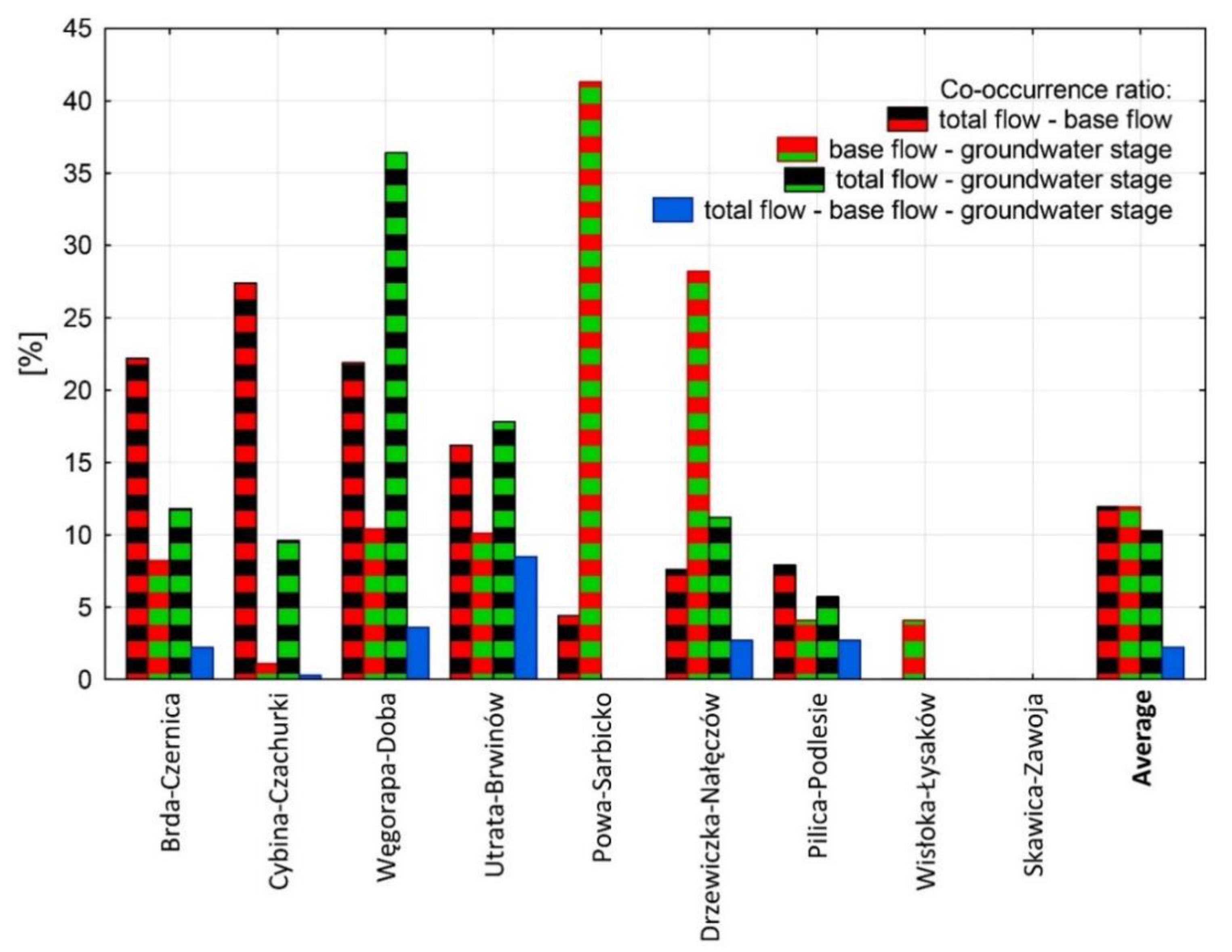
The average co-duration of a pair of the same types of hydrological season in a catchment is similar in all three components 10–12% (Figure 10). The highest sum of share ratios between total and base flow seasons occurred in lake catchments. Base flow and groundwater stage reflected very high synchronicity in the Powa and Drzewiczka catchments, which is determined mainly by a homogeneous hydrogeological structure as well as the small size of catchment areas. Good correlations in the same types of seasons between total flow and groundwater stage appeared in the Węgorapa catchment where co-duration lasted more than 1/3 of a year. A simultaneous appearance of three of the same types of hydrological season is characterized by much lower share index—2.2% on average. The highest ratio occurred in the lowland Utrata catchment (8.5%) where the depth of the groundwater table is very small (0.6 m, Table 1) and physiographic as well as hydrometeorological conditions do not differ very much.
4. Conclusions
The analysis carried out revealed that the taxonomical procedure of hydrological seasons identification, based on the assessment of the quantity, variability, and randomness of daily flows (stages) generates significant differentiation of the appearing types of seasons in a spatial and temporal pattern. Each of the identified hydrological seasons might occur only once or a few times during a year. As a result, a relatively complicated pattern of seasons according to total flow, base flow, and groundwater stage was noticed within every catchment. Analyses leading to the decomposition and identification of the determinants of the length of hydrological seasons, their frequency, and seasonal differentiation could expand knowledge of the hydrological regime, especially in dynamic matter as well as providing effective support for many water management strategies concerning the use of river and groundwater disposable resources.
The applied methodology allowed 19 types of basic hydrological seasons to be identified in the investigated group of catchments. Periods which did not satisfy the established selection criteria were taken as transitional seasons and consisted of days of mixed types. Their share in a year indicates the stability of a hydrological regime and its determinants which are mostly related to physiographical conditions where, in extreme cases, in mountainous catchments it may reach 97%, whereas in lake districts this ratio is equal to 0%.
Synchronicity and relationships between basic hydrological season types of the same features in river flows and groundwater stages analyzed on the basis of the percentage share of the number of common days with the same type of season in relation to the number of days during a year revealed some regularities. Co-occurrence of the same type of total and base flow seasons in winter–spring time in many catchments was caused by main groundwater alimentation by the river channel which is stable in multiyear and determines the whole river discharge. In the case of relation base flow—groundwater stage, co-duration in the same types of season seems to be a result of spring, stable in multiyear, the main period of groundwater elevation and its drainage by river channels in such catchments where the sampled aquifers are the main groundwater resources in alimentation processes which are related to a relatively simple hydrogeological structure of the river basin. Summer–autumn water shortage periods are also reflected in relations of base flow—groundwater stage and total flow—groundwater stage. Co-occurring types of hydrological seasons are highly variable in multiyear. This is determined by the high changeability of precipitation and evapotranspiration on a multiannual scale.
The obtained results do not always give a precise answer with respect to the origin of the observed regularities and changes as well as their directions. However, the attempt to make the procedure of hydrological seasons identification less subjective, and the conclusions concerning the frequency and distribution of seasons during a year indicate that further investigation in this field should be continued.
Author Contributions
Conceptualization, P.T. and E.T.; methodology, P.T. and E.T.; software, P.T., E.T., D.W. and L.S.; validation, P.T. and E.T.; formal analysis, P.T. and E.T.; investigation, P.T. and E.T.; resources, P.T., E.T., D.W. and L.S.; writing—original draft preparation, P.T. and E.T.; writing—review and editing, P.T. and E.T.; visualization, P.T., E.T., D.W. and L.S. All authors have read and agreed to the published version of the manuscript.
Funding
This research received no external funding.
Institutional Review Board Statement
Not applicable.
Informed Consent Statement
Not applicable.
Data Availability Statement
Publicly available datasets were analyzed in this study. This data can be found here: http://danepubliczne.imgw.pl/data/dane_pomiarowo_obserwacyjne/.
Conflicts of Interest
The authors declare no conflict of interest.
References
- Stachý, J. Wet and dry years occurrence in Poland (1951–2008). Gospod. Wodna 2011, 8, 13–321. (In Polish) [Google Scholar]
- Huang, X.R.; Zhao, J.W.; Yang, P.P. Wet-dry runoff correlation in western route of south-to-north water diversion project, China. J. Mt. Sci. 2015, 12, 592–603. [Google Scholar] [CrossRef]
- Hua, W.; She, D.; Xia, J.; He, B.; Hu, C. Dominant patterns of dryness/wetness variability in the Huang-Huai-Hai River Basin and its relationship with multiscale climate oscillations. Atmos. Res. 2021, 247, 1–13. [Google Scholar] [CrossRef]
- Markham, C.G. Seasonality in the Precipitation in The United States. Ann. Assoc. Am. Geogr. 1970, 60, 593–597. [Google Scholar] [CrossRef]
- Oliver, J.E. Monthly precipitation distribution: A comparative index. Prof. Geogr. 1980, 32, 300–309. [Google Scholar] [CrossRef]
- McCabe, G.J.; Clark, M.P. Trend and variability in Snowmelt Runoff in the Western United States. J. Hydrometeorol. 2005, 6, 476–482. [Google Scholar] [CrossRef] [Green Version]
- Haines, A.T.; Finlayson, B.L.; McMahon, T.A. A global classification of river regimes. Appl. Geogr. 1988, 8, 255–272. [Google Scholar]
- Harris, N.M.; Gurnel, A.; Hannah, D.M.; Petts, G.E. Classification of River Regimes: A Context for Hydroecology. Hydrol. Process. 2000, 14, 2831–2848. [Google Scholar] [CrossRef]
- Rotnicka, J. Theoretical foundations for separating hydrological periods and river regime analysis on the example of the Prosna River. Pr. Kom. Geogr. Geol. Ptpn 1977, XVIII, 1–94. (In Polish) [Google Scholar]
- Rotnicka, J. Taxonomic foundations of the classification of river regime. Wyd. Uam Ser. Geogr. 1988, 40, 1–238. (In Polish) [Google Scholar]
- Jokiel, P.; Tomalski, P. Attempt to determine hydrological seasons in annual hydrographs of chosen rivers in central Poland. Monogr. Kom. Gospod. Wodnej Pan 2014, 20, 203–217. (In Polish) [Google Scholar]
- Chiaudani, A.; Di Curzio, D.; Rusi, S. The snow and rainfall impact on the Verde spring behavior: A statistical approach on hydrodynamic and hydrochemical daily time-series. Sci. Total Environ. 2019, 689, 481–493. [Google Scholar] [CrossRef] [PubMed]
- Hussein, H. The Guarani Aquifer System, highly present but not high profile: A hydropolitical analysis of transboundary groundwater governance. Environ. Sci. Policy 2018, 83, 54–62. [Google Scholar] [CrossRef] [Green Version]
- da Silva, L.P.B.; Hussein, H. Production of scale in regional hydropolitics: An analysis of La Plata River Basin and the Guarani Aquifer System in South America. Geoforum 2019, 99, 42–53. [Google Scholar] [CrossRef]
- Tomaszewski, E. Seasonal changes of groundwater flow in Poland in the period 1971–1990. Acta Geogr. Lodz. 2001, 79, 1–149. (In Polish) [Google Scholar]
- White, K.E.; Sloto, R.A. Base-flow-frequency characteristics of selected Pennsylvania streams. In U.S. Geological Survey—Water-Resources Investigations Report 90-4160; USGS: Lemoyne, PA, USA, 1996; pp. 1–67. [Google Scholar]
- Sloto, R.A.; Crouse, M.Y. HYSEP: A computer program for streamflow hydrograph separation and analysis. In U.S. Geological Survey—Water-Resources Investigations Report 96-4040; USGS: Lemoyne, PA, USA, 1996; pp. 1–46. [Google Scholar]
- Ljung, G.M.; Box, G.A.P. On a Measure of a Lack of Fit in Time Series Models. Biometrica 1978, 65, 297–303. [Google Scholar] [CrossRef]
- Glantz, S.A.; Sklinker, B.K.; Neilands, T.B. Primer of Applied Regression & Analysis of Variance, 3rd ed.; McGraw Hill: New York, NY, USA, 2016; pp. 1–1216. [Google Scholar]
- Kreyszig, E. Advanced Engineering Mathematics, 4th ed.; Willey Press: New York, NY, USA, 1979; pp. 1–880. [Google Scholar]
- Ward, J.H. Hierarchical Grouping to optimize an objective function. J. Am. Stat. Assoc. 1963, 58, 236–244. [Google Scholar] [CrossRef]
- Kaufman, L.; Rousseeuw, P.J. Finding Groups in Data: An Introduction to Cluster Analysis, 2nd ed.; Willey Press: New York, NY, USA, 2005; pp. 1–342. [Google Scholar]
- Ramachandra Rao, A.; Srnivas, V.V. Regionalization of watersheds by hybrid-cluster analysis. J. Hydrol. 2006, 318, 37–56. [Google Scholar] [CrossRef]
- Wrzesiński, D. Detection of changes in the hydrological regime of the Warta in the Poznań profile in 1822–2005. In Odpływ Rzeczny i Jego Regionalne Uwarunkowania, 1st ed.; Wrzesiński, D., Ed.; Bogucki Wydawnictwo Naukowe: Poznań, Poland, 2010; pp. 135–152. (In Polish) [Google Scholar]
- Everitt, B.S.; Landau, S.; Leese, M.; Stahl, D. Cluster Analysis, 5th ed.; Willey Press: New York, NY, USA, 2011; pp. 1–346. [Google Scholar]
- Wrzesiński, D.; Sobkowiak, L. Detection of changes in flow regime of rivers in Poland. J. Hydrol. Hydromech. 2018, 66, 55–64. [Google Scholar] [CrossRef] [Green Version]
- Wrzesiński, D.; Sobkowiak, L. Transformation of the Flow Regime of a Large Allochthonous River in Central Europe—An Example of the Vistula River in Poland. Water 2020, 12, 507. [Google Scholar] [CrossRef] [Green Version]
- Graf, R.; Wrzesiński, D. Detecting Patterns of Changes in River Water Temperature in Poland. Water 2020, 12, 1327. [Google Scholar] [CrossRef]
- Rousseeuw, P.J. Silhouettes: A Graphical Aid to the Interpretation and Validation of Cluster Analysis. Comput. Appl. Math. 1987, 20, 53–65. [Google Scholar] [CrossRef] [Green Version]
- Sugar, C.A.; James, G.M. Finding the Number of Clusters in a Dataset: An Information-Theoretic Approach. J. Am. Stat. Assoc. 2003, 98, 750–763. [Google Scholar] [CrossRef]
- Mojena, R. Hierarchical grouping methods and stopping rules: An evaluation. Comput. J. 1977, 20, 359–363. [Google Scholar] [CrossRef] [Green Version]
- Milligan, G.W.; Cooper, M.C. An Examination of Procedures for Determining the Number of Clusters in a Data Set. Psychometrica 1985, 50, 159–179. [Google Scholar] [CrossRef]
- Jokiel, P.; Tomalski, P. Transformations of hydrological seasons configuration along the Vistula and the Oder river. Monogr. Kom. Gospod. Wodnej Pan 2019, 42, 21–33. (In Polish) [Google Scholar]
- Sujono, J.; Shikasho, S.; Hiramatsu, K. A comparison of techniques for hydrograph recession analysis. Hydrol. Process. 2004, 18, 403–413. [Google Scholar] [CrossRef]
- Brandes, D.; Hoffmann, J.G.; Mangarillo, J.T. Base Flow Recession Rates, Low Flows, and Hydrologic Features of Small Watersheds in Pennsylvania, USA. J. Am. Water Resour. Assoc. 2005, 41, 1177–1186. [Google Scholar] [CrossRef]
- Tallaksen, L.M. A review of baseflow recession analysis. J. Hydrol. 1995, 165, 349–370. [Google Scholar] [CrossRef]
- Smakhtin, V.U. Low flow hydrology: A review. J. Hydrol. 2001, 240, 147–186. [Google Scholar] [CrossRef]
- Balek, J. Groundwater Resources Assessment, 1st ed.; Developments in Water Science; Elsevier: Amsterdam, The Netherlands, 1989; Volume 38, pp. 1–249. [Google Scholar]
Figure 1.
Location of studied catchments. Note: numbering of water gauges in accordance with Table 1.
Figure 1.
Location of studied catchments. Note: numbering of water gauges in accordance with Table 1.

Figure 2.
An example of daily flow hydrograph separation.

Figure 3.
An example of annual course of recalculated series of average river flows and groundwater stages, its variability and autocorrelation in single-name day step in the multiyear. Notes: Q—river discharge; H—groundwater stage; Cv—variation coefficient; Ra—autocorrelation coefficient.
Figure 3.
An example of annual course of recalculated series of average river flows and groundwater stages, its variability and autocorrelation in single-name day step in the multiyear. Notes: Q—river discharge; H—groundwater stage; Cv—variation coefficient; Ra—autocorrelation coefficient.

Figure 4.
Scheme of type of day identification. Notes: δ—standard deviation; Racr—autocorrelation coefficient at critical values of Box–Ljung test (α = 0.05).
Figure 4.
Scheme of type of day identification. Notes: δ—standard deviation; Racr—autocorrelation coefficient at critical values of Box–Ljung test (α = 0.05).

Figure 5.
An example of delimitation of hydrological seasons in base flow series.

Figure 6.
Annual course of identified hydrological seasons in studied catchments. Notes: TF—total flow; BF—base flow; GS—groundwater stage; TRANS—transitional hydrological seasons; the other symbols in accordance with Table 2 and Figure 4.

Figure 7.
Table of convergence of identified types of basic hydrological seasons. Time series: in black—total flow; in red—base flow; in green—groundwater stage. Multiannual variable tendency: R—rhythm; T—trend; S—stochastic.
Figure 7.
Table of convergence of identified types of basic hydrological seasons. Time series: in black—total flow; in red—base flow; in green—groundwater stage. Multiannual variable tendency: R—rhythm; T—trend; S—stochastic.

Figure 8.
Distribution of quantity (a) and variability (b) component in identified basic hydrological seasons.
Figure 8.
Distribution of quantity (a) and variability (b) component in identified basic hydrological seasons.

Figure 9.
Share of number of days with basic hydrological season in number of days in the whole year.
Figure 9.
Share of number of days with basic hydrological season in number of days in the whole year.

Figure 10.
Share of number of days with co-occurring basic hydrological seasons of the same type in number of days in the whole year.
Figure 10.
Share of number of days with co-occurring basic hydrological seasons of the same type in number of days in the whole year.


Table 1.
Basic characteristics of selected catchments and aquifers
| No. | Region | River | Water Gauge | A (km2) | Hav (m) | Age of Aquifer |
|---|---|---|---|---|---|---|
| 1 | Lake districts | Brda | Swornegacie | 1200.5 | 3.5 | Q |
| 2 | Lake districts | Cybina | Antoninek | 170.6 | 0.8 | Q |
| 3 | Lake districts | Węgorapa | Prynowo | 647.2 | 0.95 | Q |
| 4 | Lowlands | Utrata | Krubice | 714.7 | 0.6 | Q |
| 5 | Lowlands | Powa | Posoka | 331.5 | 5.37 | Q |
| 6 | Uplands | Drzewiczka | Opoczno | 604.7 | 0.90 | T1 + Q |
| 7 | Uplands | Pilica | Wąsosz | 994.5 | 5.8 | Cr2 |
| 8 | Mountains | Wisłoka | Mielec | 3915.3 | 7.8 | Q |
| 9 | Mountains | Skawica | Skawica Dolna | 139.3 | 1.85 | Q |
A—catchment area, Hav—average depth to groundwater table; Q—quaternary, T1—Lower Triassic; Cr2—Upper Cretaceous.
Table 2.
Types of day in studied group of catchments.
| No. | Characteristic of Types of Day | Name of the Type of Day | L | ||
|---|---|---|---|---|---|
| Quantity | Variability | Statistical Significance of Autocorrelation Coefficient | |||
| 1 | Extremely high | Extremely high | Lack of | EHQ/EHV/STOCH | 2,0,0 |
| 2 | Very high | Low | Lack of | EHQ/LV/STOCH | 2,4,1 |
| 3 | Very high | Very low | Lack of | VHQ/VLV/STOCH | 0,0,1 |
| 4 | High | Very high | Lack of | HQ/VHV/STOCH | 3,1,2 |
| 5 | High | High | Lack of | HQ/HV/STOCH | 3,1,0 |
| 6 | High | Average | Lack of | HQ/AV/STOCH | 3,4,5 |
| 7 | High | Average | Negative | HQ/AV/RHYTHM | 0,0,1 |
| 8 | High | Low | Lack of | HQ/LV/STOCH | 6,4,5 |
| 9 | High | Very low | Negative | HQ/VLV/RHYTHM | 0,1,0 |
| 10 | Average | Very high | Lack of | AQ/VHV/STOCH | 0,2,0 |
| 11 | Average | High | Lack of | AQ/HV/STOCH | 2,2,2 |
| 12 | Average | Average | Lack of | AQ/AV/STOCH | 5,7,4 |
| 13 | Average | Low | Lack of | AQ/LV/STOCH | 5,2,4 |
| 14 | Low | Very high | Lack of | LQ/VHV/STOCH | 1,3,0 |
| 15 | Low | High | Lack of | LQ/HV/STOCH | 3,4,5 |
| 16 | Low | Average | Lack of | LQ/AV/STOCH | 6,7,4 |
| 17 | Low | Average | Positive | LQ/AV/TREND | 0,1,0 |
| 18 | Low | Low | Lack of | LQ/LV/STOCH | 3,3,2 |
| 19 | Low | Low | Negative | LQ/LV/RHYTHM | 0,0,1 |
| 20 | Very low | High | Lack of | VLQ/HV/STOCH | 0,0,1 |
| 21 | Very low | Average | Lack of | VLQ/AV/STOCH | 1,0,0 |
L—number of water gauges (groundwater stations) where particular types of day was identified in times series of total flow, base flow, groundwater stages; names of type of day in bold did not satisfy critical length for basic hydrological season.
Table 3.
Characteristics of established hydrological seasons in examined catchments.
| No. | Catchment | Number of Days of Transitional Hydrological Season During a Year (Percentage) | Critical Length of Basic Hydrological Season (Days) | Number of Identified Basic Hydrological Seasons | ||||||
|---|---|---|---|---|---|---|---|---|---|---|
| TF | BF | GS | TF | BF | GS | TF | BF | GS | ||
| 1 | Brda | 9 (2) | 0 (0) | 77 (21) | 9 | 8 | 9 | 5 | 5 | 5 |
| 2 | Cybina | 11 (3) | 0 (0) | 0 (0) | 9 | 5 | 38 | 5 | 5 | 3 |
| 3 | Węgorapa | 3 (1) | 13 (4) | 0 (0) | 11 | 11 | 10 | 4 | 5 | 4 |
| 4 | Utrata | 126 (35) | 8 (2) | 0 (0) | 9 | 5 | 9 | 5 | 5 | 5 |
| 5 | Powa | 212 (58) | 0 (0) | 41(11) | 10 | 6 | 16 | 5 | 6 | 4 |
| 6 | Drzewiczka | 187 (51) | 0 (0) | 21 (6) | 6 | 7 | 13 | 5 | 5 | 4 |
| 7 | Pilica | 204 (56) | 4 (1) | 1 (0) | 3 | 7 | 11 | 6 | 5 | 4 |
| 8 | Wisłoka | 267 (73) | 10 (3) | 92 (25) | 8 | 14 | 19 | 5 | 4 | 4 |
| 9 | Skawica | 353 (97) | 8 (2) | 343 (94) | 3 | 7 | 10 | 6 | 6 | 5 |
TF—total flow; BF—base flow; GS—groundwater stage.
Table 4.
Share of number of days with co-occurring basic hydrological seasons of the same type in number of days in the whole year (%).
Table 4.
Share of number of days with co-occurring basic hydrological seasons of the same type in number of days in the whole year (%).
| Type | Brda-Czernica | Cybina-Czachurki | Węgorapa-Doba | Utrata-Brwinów | Powa-Sarbicko | Drzewiczka-Nałęczów | Pilica-Podlesie | Wisłoka-Łysaków | Skawica-Zawoja |
|---|---|---|---|---|---|---|---|---|---|
| total flow—base flow | |||||||||
| EHQ/LV/STOCH | 12.1 | 11.2 | |||||||
| HQ/VHV/STOCH | 3.3 | ||||||||
| HQ/AV/STOCH | 22.2 | 4.9 | |||||||
| HQ/LV/STOCH | 11 | 2.7 | 0.8 | ||||||
| AQ/HV/STOCH | 0 | ||||||||
| AQ/AV/STOCH | 10.7 | 7.1 | 0 | ||||||
| AQ/LV/STOCH | 14.5 | ||||||||
| LQ/AV/STOCH | 0.8 | 5.2 | 1.1 | 0 | |||||
| base flow—groundwater stage | |||||||||
| HQ/AV/STOCH | 2.2 | 1.4 | |||||||
| HQ/LV/STOCH | 8.5 | 22.7 | 12.3 | ||||||
| AQ/HV/STOCH | 4.1 | ||||||||
| AQ/AV/STOCH | 3.6 | 1.6 | 4.1 | 0 | |||||
| AQ/LV/STOCH | 1.1 | 6.8 | |||||||
| LQ/HV/STOCH | 14.5 | ||||||||
| LQ/AV/STOCH | 6 | 11.2 | 0 | ||||||
| LQ/LV/STOCH | 7.4 | ||||||||
| total flow—groundwater stage | |||||||||
| HQ/AV/STOCH | 11.8 | 2.2 | |||||||
| HQ/LV/STOCH | 0 | 8.5 | 2.7 | 0 | |||||
| AQ/AV/STOCH | 16.7 | 2.7 | |||||||
| AQ/LV/STOCH | 0.3 | ||||||||
| LQ/HV/STOCH | 9.3 | 19.7 | 9.3 | ||||||
| LQ/AV/STOCH | 0 | 6.3 | 3 | ||||||
| total flow—base flow—groundwater stage | |||||||||
| HQ/AV/LOS | 2.2 | 0 | |||||||
| HQ/LV/LOS | 8.5 | 2.7 | |||||||
| AQ/AV/LOS | 3.6 | 2.7 | |||||||
| AQ/LV/LOS | 0.3 | ||||||||
| LQ/AV/LOS | 0 | 0 | |||||||
Symbols of types in accordance with Table 2. Value of “0” means that seasons of the same type appeared, however, they did not co-occur.
Publisher’s Note: MDPI stays neutral with regard to jurisdictional claims in published maps and institutional affiliations. |
© 2021 by the authors. Licensee MDPI, Basel, Switzerland. This article is an open access article distributed under the terms and conditions of the Creative Commons Attribution (CC BY) license (http://creativecommons.org/licenses/by/4.0/).
Share and Cite
MDPI and ACS Style
Tomalski, P.; Tomaszewski, E.; Wrzesiński, D.; Sobkowiak, L. Relationships of Hydrological Seasons in Rivers and Groundwaters in Selected Catchments in Poland. Water 2021, 13, 250. https://doi.org/10.3390/w13030250
AMA Style
Tomalski P, Tomaszewski E, Wrzesiński D, Sobkowiak L. Relationships of Hydrological Seasons in Rivers and Groundwaters in Selected Catchments in Poland. Water. 2021; 13(3):250. https://doi.org/10.3390/w13030250
Chicago/Turabian StyleTomalski, Przemysław, Edmund Tomaszewski, Dariusz Wrzesiński, and Leszek Sobkowiak. 2021. "Relationships of Hydrological Seasons in Rivers and Groundwaters in Selected Catchments in Poland" Water 13, no. 3: 250. https://doi.org/10.3390/w13030250
Note that from the first issue of 2016, this journal uses article numbers instead of page numbers. See further details here.