
Changing Water Levels in Lake Superior, MI (USA) Impact Periphytic Diatom Assemblages in the Keweenaw Peninsula


1
Department of Biology, Grand Valley State University, Allendale, MI 49401, USA
2
Department of Natural Resource Ecology and Management, Iowa State University, Ames, IA 50011, USA
3
Department of Biology, Waubonsee Community College, Sugar Grove, IL 60554, USA
*
Author to whom correspondence should be addressed.
Water 2021, 13(3), 253; https://doi.org/10.3390/w13030253
Submission received: 23 November 2020
/
Revised: 4 January 2021
/
Accepted: 18 January 2021
/
Published: 20 January 2021
(This article belongs to the Special Issue Climate Change and Water Levels in the Great Lakes)
Abstract
:Predicted climate-induced changes in the Great Lakes include increased variability in water levels, which may shift periphyton habitat. Our goal was to determine the impacts of water level changes in Lake Superior on the periphyton community assemblages in the Keweenaw Peninsula with different surface geology. At three sites, we identified periphyton assemblages as a function of depth, determined surface area of periphyton habitat using high resolution bathymetry, and estimated the impact of water level changes in Lake Superior on periphyton habitat. Our results suggest that substrate geology influences periphyton community assemblages in the Keweenaw Peninsula. Using predicted changes in water levels, we found that a decrease in levels of 0.63 m resulted in a loss of available surface area for periphyton habitat by 600 to 3000 m2 per 100 m of shoreline with slopes ranging 2 to 9°. If water levels rise, the surface area of substrate will increase by 150 to 370 m2 per 100 m of shoreline, as the slopes above the lake levels are steeper (8–20°). Since periphyton communities vary per site, changes in the surface area of the substrate will likely result in a shift in species composition, which could alter the structure of aquatic food webs and ecological processes.
1. Introduction
Since the 1950s, the climate of the Great Lakes continues to change: air temperatures have increased by 1.3 °C, precipitation has increased 14% with less snow and more rain, and summer lake surface temperatures have increased by 2.5 °C [1]. Models predict that climate-induced changes in the Great Lakes include an increased variability in lake levels [2]. For instance, water levels in Lake Michigan and Lake Huron are nearly 1 m higher compared to the long-term average since 1918 [3]. Levels in Lake Superior and Lake Erie are also higher than historical records [3]. Fluctuating water levels fundamentally affect the biophysical and chemical properties of the Great Lakes [4] including lake circulation, aquatic communities, ecosystem productivity, fish and wildlife habitat quality, and the availability and quality of water for human use [5,6,7]. In particular, microbial communities in aquatic ecosystems may quickly change in response to increased air and water temperatures. For instance, warmer water temperatures may change the composition of periphyton communities, which then may disturb ecological processes and function.
Periphyton communities are diverse and include photosynthetic organisms such as diatoms, green algae, and cyanobacteria, which are found attached to benthic substrates in aquatic ecosystems. As primary producers, they form the base of many aquatic food webs, providing fixed carbon to numerous trophic levels both directly and indirectly. Periphyton are often used in bioassessment (see [8] for review) in part because of their role in food webs, their high diversity and species richness in small samples [9], and their variable community structure based on the chemical and physical environment. Nutrient type and concentration influence periphyton community composition, with specific taxa promoted with the additions of nitrogen and phosphorus [10]. Diatoms in particular are commonly used as bioindicators because they are both diverse and sensitive to nutrients [10]. The physical structure of aquatic environments, including size of rocks [11], stone roughness [12] and refuge from disturbance [13] influence periphyton community composition and biomass [14,15]. Previous research investigating periphyton communities has documented distinct changes in relation to geology. For example, in southeast Brazil, researchers [16] found decreases in the relative biovolume of diatoms, with concurrent increases in green algae with increasing surface roughness. More specifically, they found decreases in taxa that adhered to surfaces using pads and stalks, such as Eunotia flexuosa (Brébisson) Kützing and Gomphonema gracile (Ehrenberg), with greater surface roughness. Despite changes in community composition, there were similar values of diversity, richness and evenness in periphyton communities of various surface roughness [16].
The purpose of this study was to determine the impact of water level changes in Lake Superior on periphyton community assemblages in areas of the Keweenaw Peninsula with different subsurface geology. At three locations in the Keweenaw Peninsula, all with variable geology, we had the following objectives: (1) determine periphyton community assemblages as a function of depth, (2) determine surface area of periphyton habitat using high resolution bathymetry, and (3) determine the potential impacts of shifting lake levels on periphyton habitat and community assemblages based on forecasts for Lake Superior [17,18].
2. Materials and Methods
2.1. Site Location
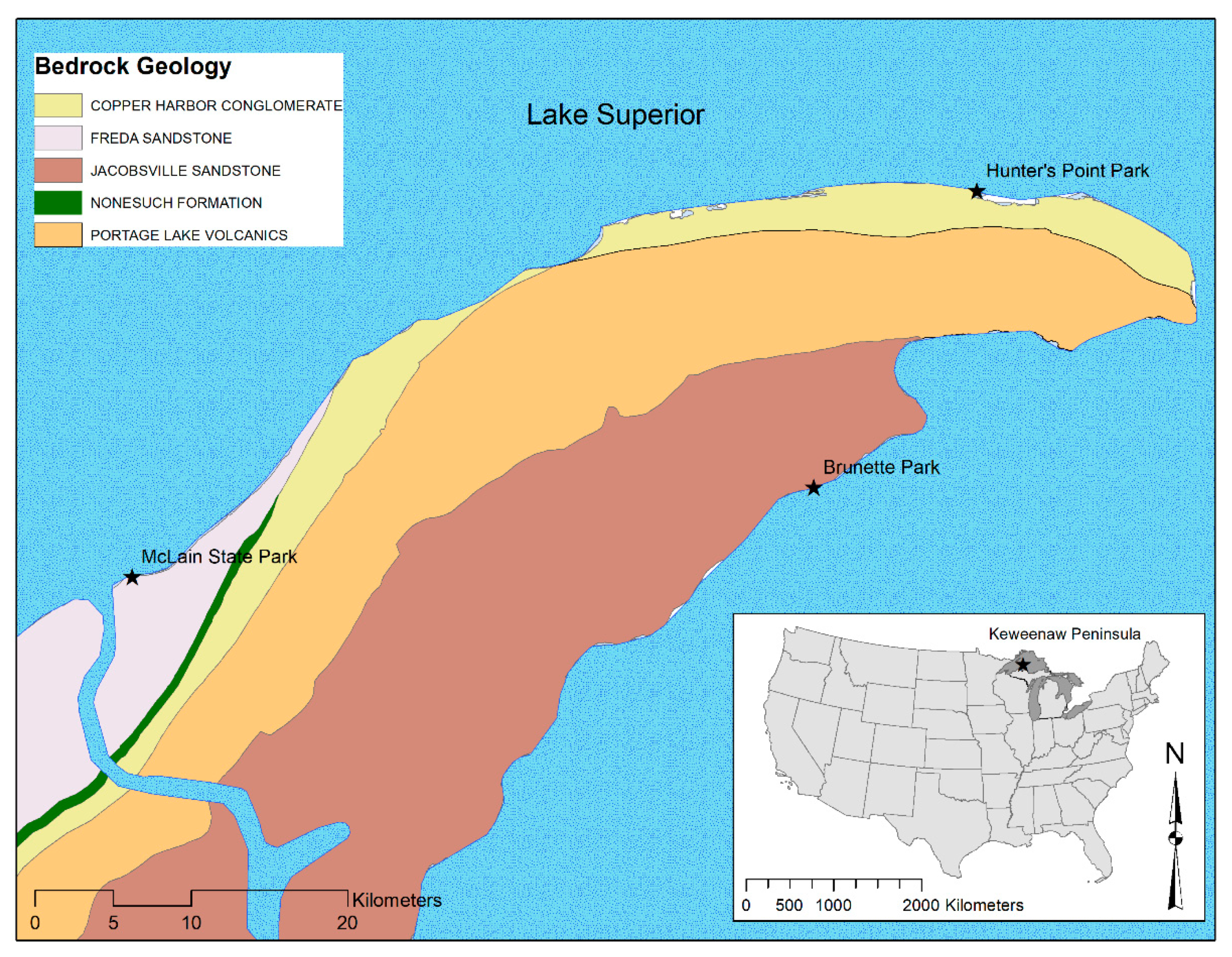
The Keweenaw Peninsula in Lake Superior contains diverse geology in a relatively small geographic area (1455 km2; Figure 1). In the small area we expected similar air and water temperatures and nutrient (phosphorus and nitrogen) concentrations. Because temperature and nutrients influence periphyton growth, this location provided an opportunity to compare periphyton community assemblages as a function of geology and microtopography. We selected three sites in the Keweenaw Peninsula based on nearshore geology and accessibility: McLain State Park (ML) had loose sand and gravel with patches of Freda Sandstone bedrock; Hunter’s Point Park (HP) contained basalt andesite lava flows and Copper Harbor Conglomerate with rhyolitic pebble; and Brunette Park (BP) was Jacobsville Sandstone with some loose sand and gravel [19]. At each site, we delineated three transects for fieldwork, that were approximately 60 m apart. Three sampling locations per transect at three repetitive depths (z = 0, z = 1 m and z = 2 m; 27 total locations), were studied. Each transect began at the shoreline (elevation = 183.5 m) and extended into the water perpendicular to the shore to a maximum depth of 2 m. These depths were all within the euphotic zone of Lake Superior (42 ± 2 m; [20]), as well as the water mixing zone, since nearshore depths are those likely influenced by a change in lake level.
2.2. Sample Collection
At each sampling location, we collected water for nutrients and physical data, along with periphyton samples from directly above or from the lake bottom from 10 to 13 August 2019. Whole water samples (250 mL) were collected for total phosphorus and nitrate using a VanDorn water sampler suspended directly above the lake bottom and placed into acid-washed bottles; nutrient samples were frozen the day collected and delivered to Superior Analytics (Lake Superior State University, Sault Ste Marie, MI, USA) for analyses. We used a calibrated Hydrolab multi-probed instrument to measure pH, temperature, electrolytic conductivity and dissolved oxygen by suspending the probe directly above the lake bottom. Triplicate rocks were gently collected by hand at each sampling location. In depths of 1 and 2 m, we collected rocks opportunistically in an area of approximately 25 m2. Each rock, regardless of depth, was measured (length, width, depth) to approximate surface area. Periphyton were removed from the three rocks using toothbrushes rinsed with distilled water [21] and placed into a centrifuge tube for each sampling location. These samples were placed in coolers and shipped without preservatives for the identification and quantification of diatoms. Field periphyton samples were cleaned in the lab using 5.25% sodium hypochlorite followed by rinsing and decanting with filtered water until being pH neutral [22]. Cleaned diatom frustules were mounted in Naphrax® (Brunel Microscopes, Chippenham, UK) and enumerated at 1000× using an Olympus CX31 (Olympus, Tokyo, Japan). Species identifications of at least 600 diatom valves were made using a variety of references including Krammer and Lange-Bertalot [23], Krammer and Lange-Bertalot [24], Krammer and Lange-Bertalot [25], and Krammer and Lange-Bertalot [26], and Diatoms of North America [27]. With nine sampling locations per site, this sampling effort resulted in 27 water samples for total phosphorus and nitrate, measurements of pH, water temperature, electrolytic conductivity and dissolved oxygen, and composite periphyton samples.
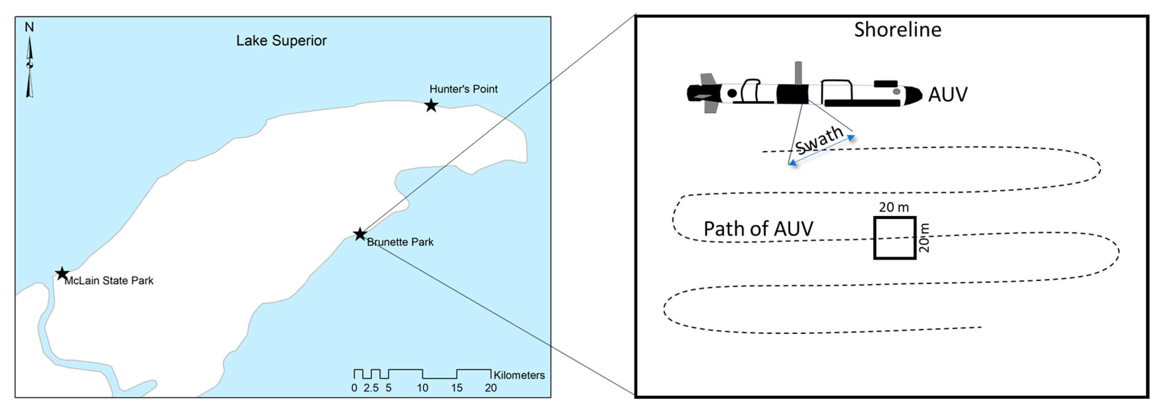
Spatial data were collected and processed by Michigan Technological University (Great Lakes Resource Center, Houghton, MI, USA) using an Iver autonomous underwater vehicle (AUV) to generate a high-resolution map depicting the structure of the lake bottom. The AUV was pre-programmed to travel back and forth within the study area and collect multibeam XYZ point locations at a rate of 1000 per second, resulting in a point cloud of depth data at a resolution of 10 cm along each swath.
2.3. Quantitative and Spatial Analyses
We used a combination of univariate, multivariate and spatial analyses to address study objectives. Total phosphorus and nitrate were compared by site and depth using a two-way ANOVA with interaction following assessment with Shapiro-Wilk and Levene’s Tests for normality and equal variance. Additional abiotic data including pH, temperature, conductivity and dissolved oxygen were compared by site using summary statistics and we used non-metric multidimensional scaling (NMDS) to examine a Bray-Curtis similarity matrix of periphytic diatom assemblages across depths and sites. The similarity of sites, depths and their interaction, as well as multiple comparisons, were compared using post hoc Adonis. All quantitative analyses were conducted using R Version 3.4.0 [28] with the packages car [29], MASS [30], and vegan [31].
To analyze the structure of the lake bottom, we implemented a hierarchical three-dimensional spatial analysis using ArcScene v 10.4.1 software [32], where the first step was to characterize each of the three study sites using 4 m topo bathymetry [33], and the second step was to characterize microtopography and surface irregularities for periphyton habitat within each of the three study sites using high-resolution data from the AUV (Figure 2). At each sample location, we used Spatial Analyst Tools to calculate slope and analyze depth from the topo bathymetry data. We calculated slope from the change in depth along three 100 m transects starting from the shoreline. Using the AUV data, we converted the XYZ files to a raster surface grid with a resolution of 30 cm to account for error in measurements between points and create a contiguous depth surface in order to quantify substrate structure and surface area. We randomly selected three 400 m2 plots within the study area in which we calculated surface area and plotted the change in depth on the surface of the substrate along a transect within the center of each plot. We modeled the amount of surface area of substrate that would be exposed in each study site location based on future projections (−0.63 m to 0.52 m; Table 1) in water levels in Lake Superior [17].
3. Results
3.1. Physical and Chemical Data
Water temperature, dissolved oxygen and conductivity were similar at all sites (Table 2). Nitrate was not significantly different by site (p = 0.1773, F2,18 = 1.9077) nor depth (p = 0.9405, F2,18 = 0.0615), nor interaction (p = 0.1063, F4,18 = 2.2308; Figure 3). In addition, total phosphorus was not significantly different by site (p = 0.5177, F2,18 = 0.6830) nor depth (p = 0.6617, F2,18 = 0.4226), nor interaction (p = 0.7017, F4,18 = 0.5497; Figure 2).
3.2. Periphytic Diatom Assemblages
Composite samples were collected for periphyton determination from three rocks at each sampling location. Mean rock surface areas, with standard errors, were similar (BP: 842.3 ± 149.7 cm2; HP: 752.4 ± 137.8 cm2; ML: 1136 ± 184.7 cm2) and up to 600 valves were identified and counted per sample. Not all samples contained periphyton, including those collected in the active wave zone at HP and ML.
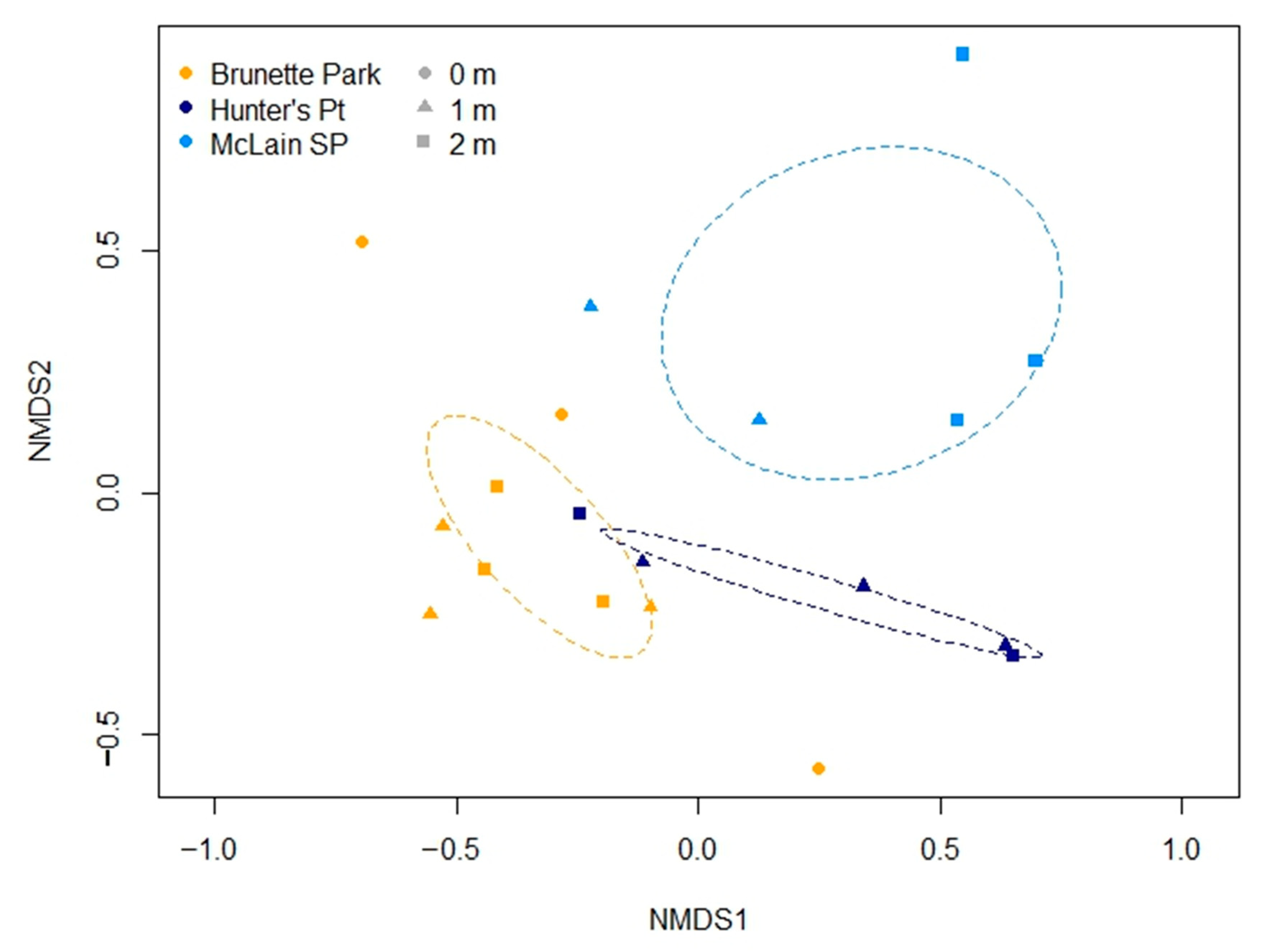
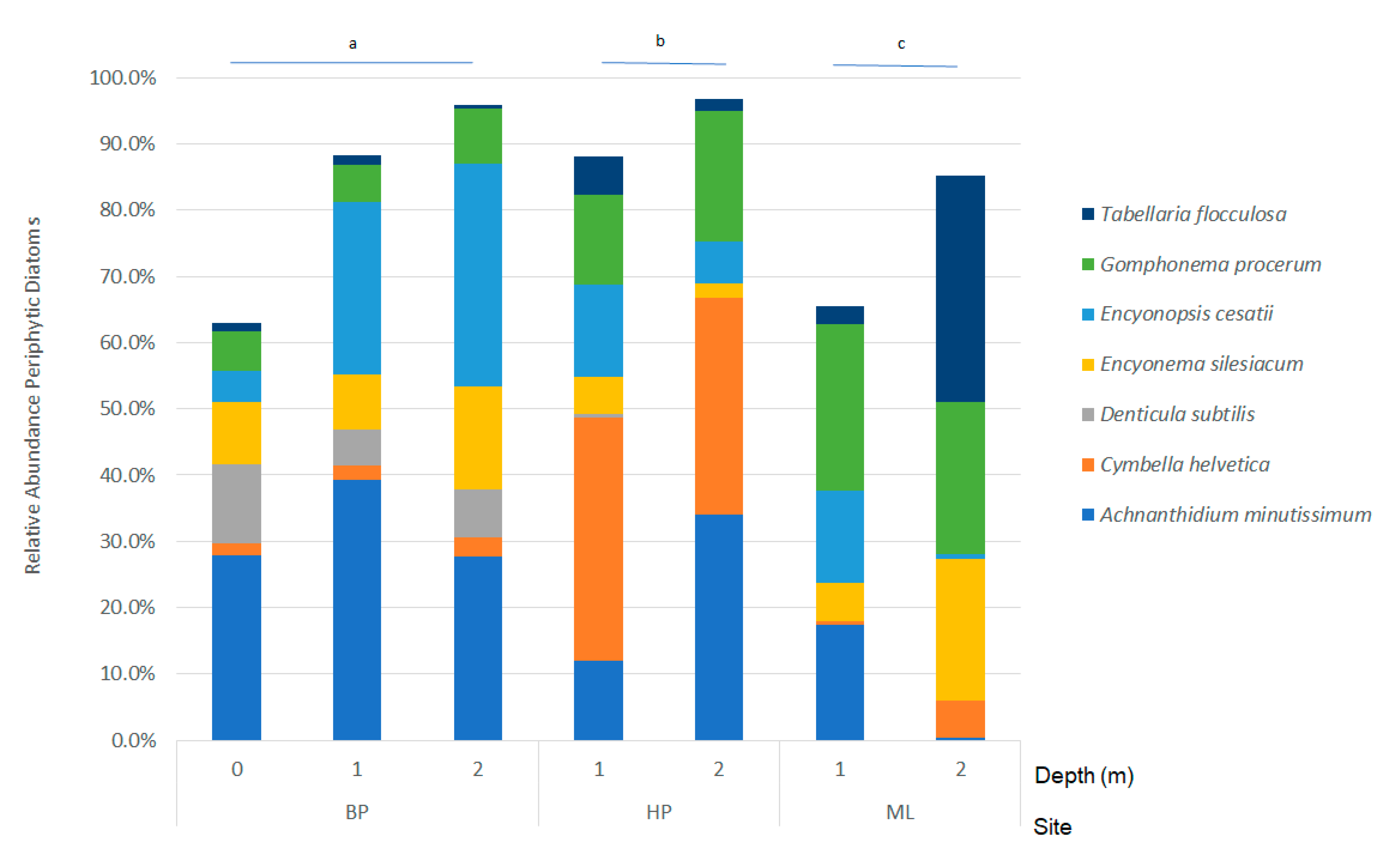
Periphyton communities were compared using non-metric multidimensional scaling of a Hellinger transformed Bray-Curtis similarity matrix (Figure 3). The lowest stress (12.84%) was achieved using the metaMDS function in vegan [31]. Post hoc Adonis indicated that communities were different based on site (p = 0.001), but neither depth (p = 0.160) nor their interaction (p = 0.187). Further, pairwise comparisons with a Holm’s adjustment revealed that all sites had significantly different periphyton communities (BP:HP, p = 0.046; BP:ML, p = 0.006; HP:ML, p = 0.046). We used similarity percentages (SIMPER) and determined the species that contributed up to 50% of the cumulative differences in sites (Figure 4). Sites at BP were characterized by high abundances of Achnanthidium minutissimum (Kützing) Czarnecki and Encyonopsis cesatii (Rabenhorst) Krammer, whereas HP contained greater Cymbella helvetica Kützing and ML was characterized by high amounts of Gomphonema procerum Reichardt and Lange-Bertalot and Tabellaria flocculosa (Roth) Kützing.
3.3. Spatial Modeling and Habitat Structure
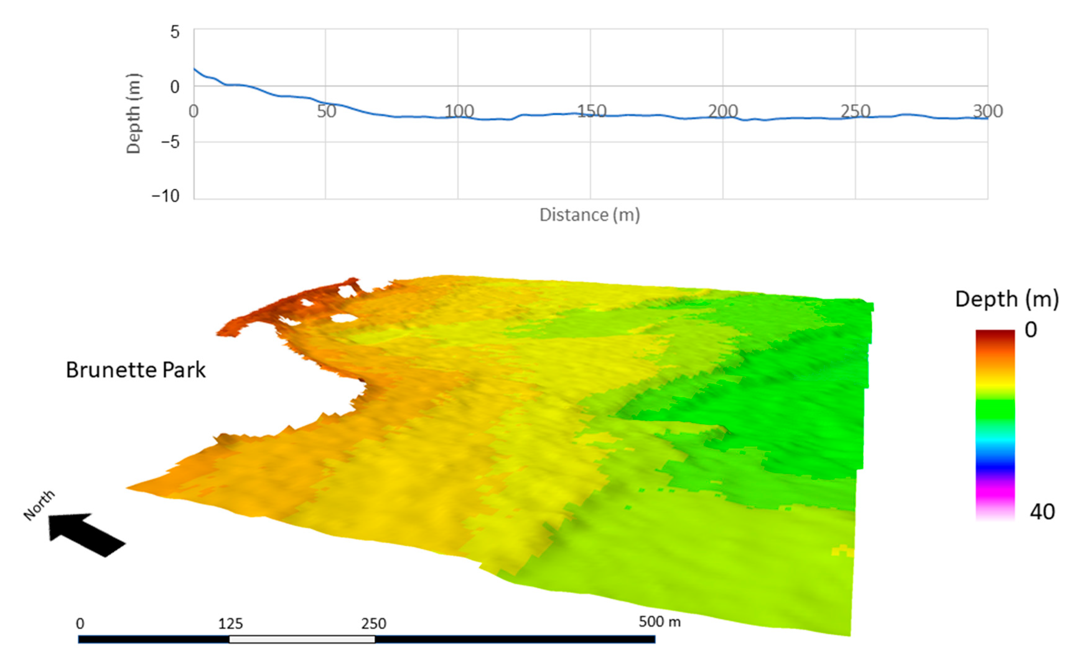
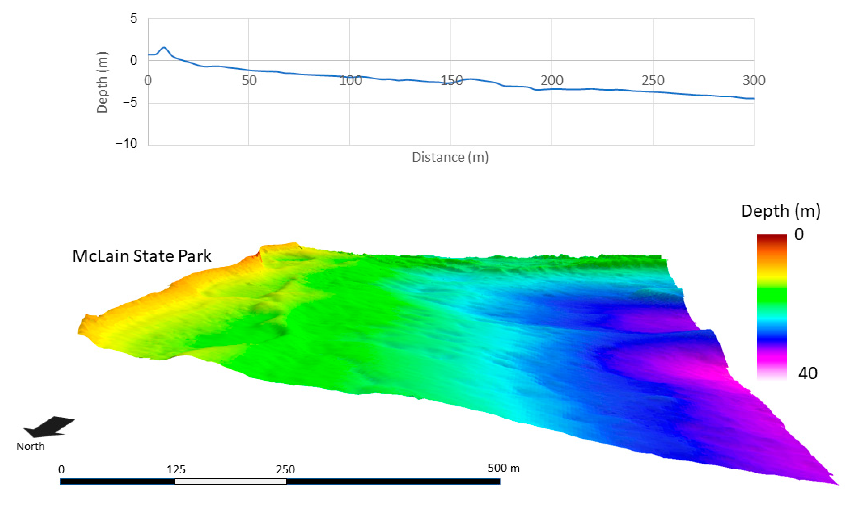
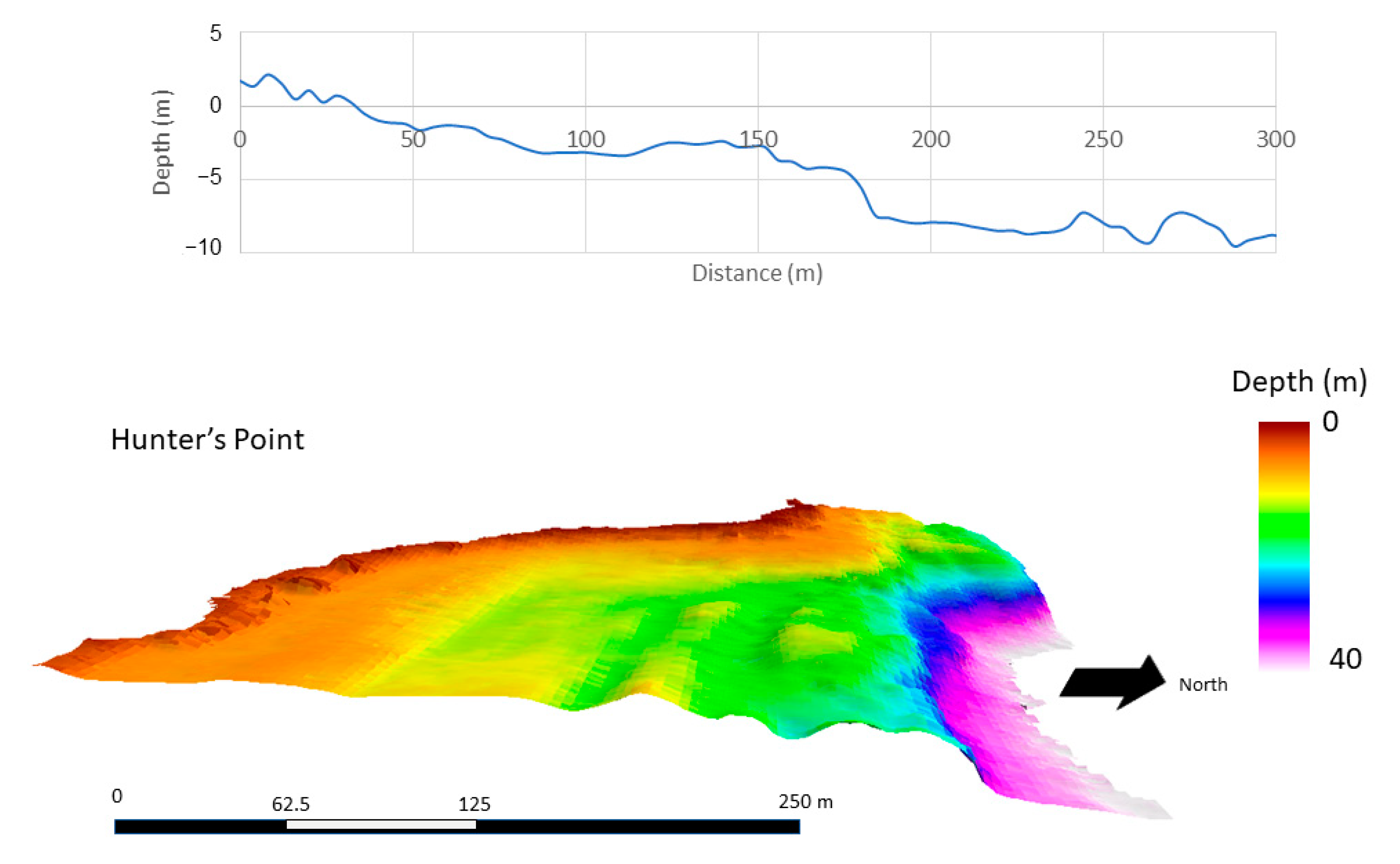
At a resolution of 4 m, substrate structure and surface area differed among the study areas. This resolution characterized the physical structure of the substrate at a broad scale. ML and BP were similar in slope and bathymetric structure (Figure 5 and Figure 6). Within the first 100 m extending from the shoreline, both ML and BP had slopes of <3° and maximum depths of <2.7 m, whereas HP had steeper and more variable slopes ranging 2 to 9° and maximum depths of <3.5 m within the first 100 m (Figure 7). Beyond 100 m, slopes increased at HP, but were not as steep at ML and BP.
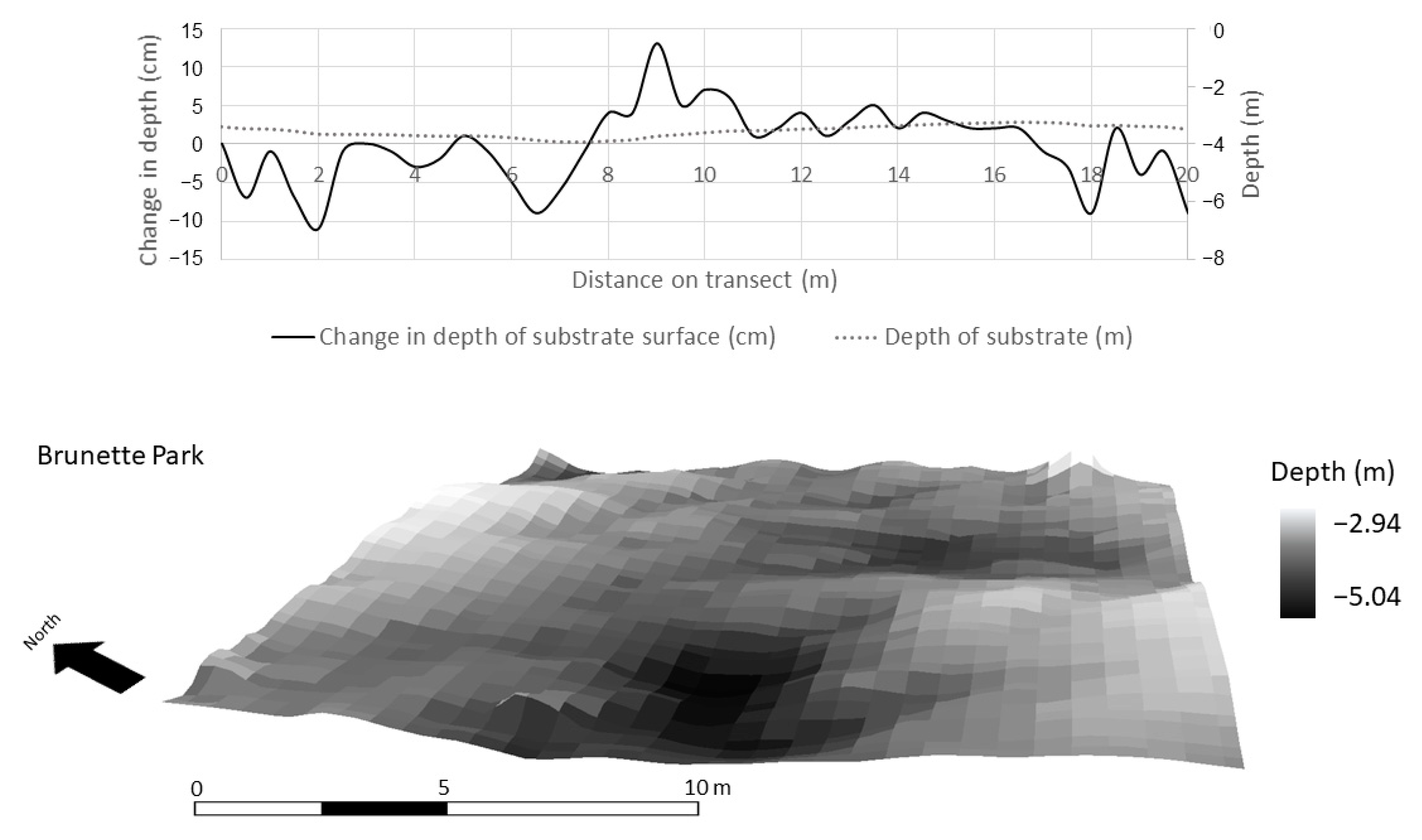
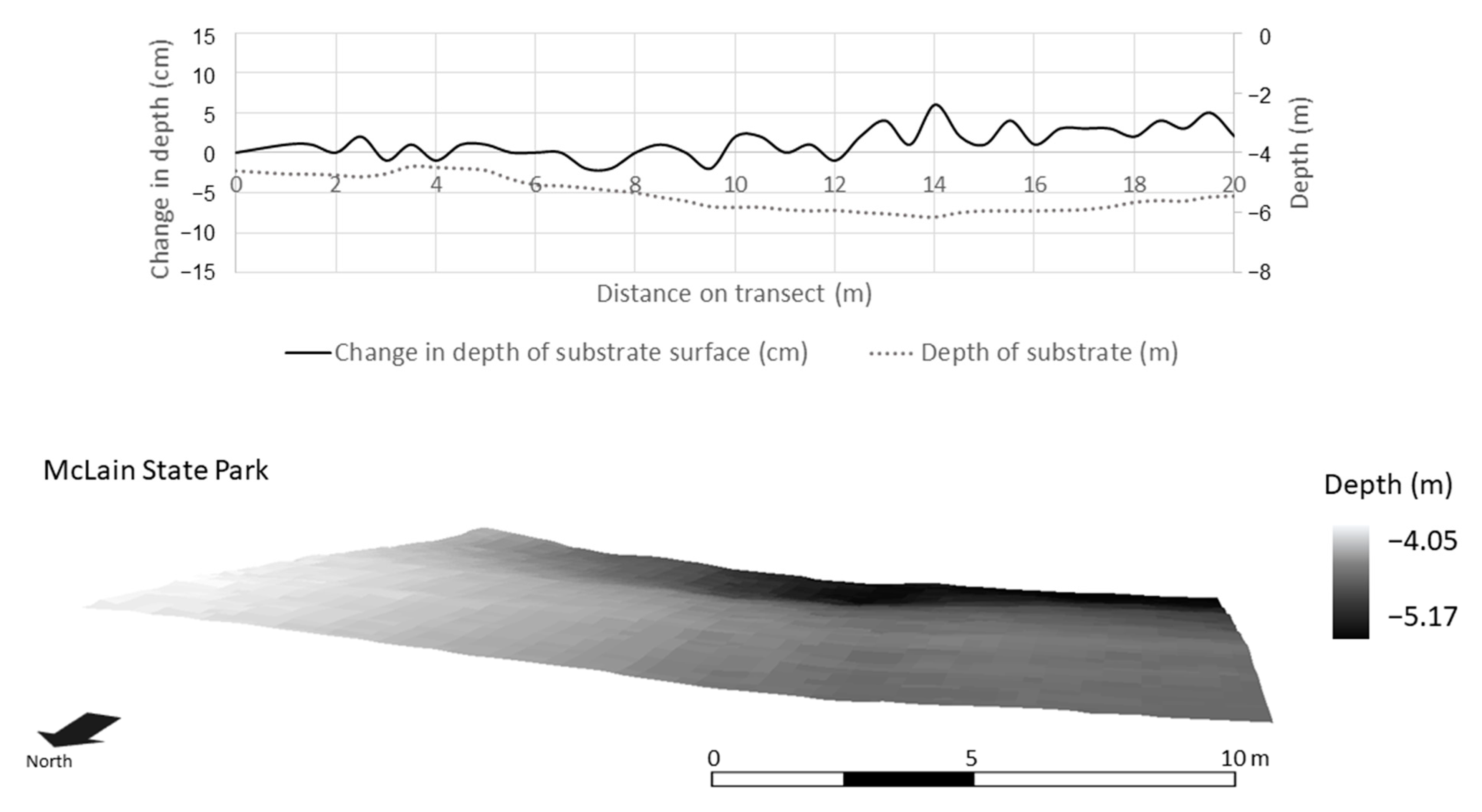
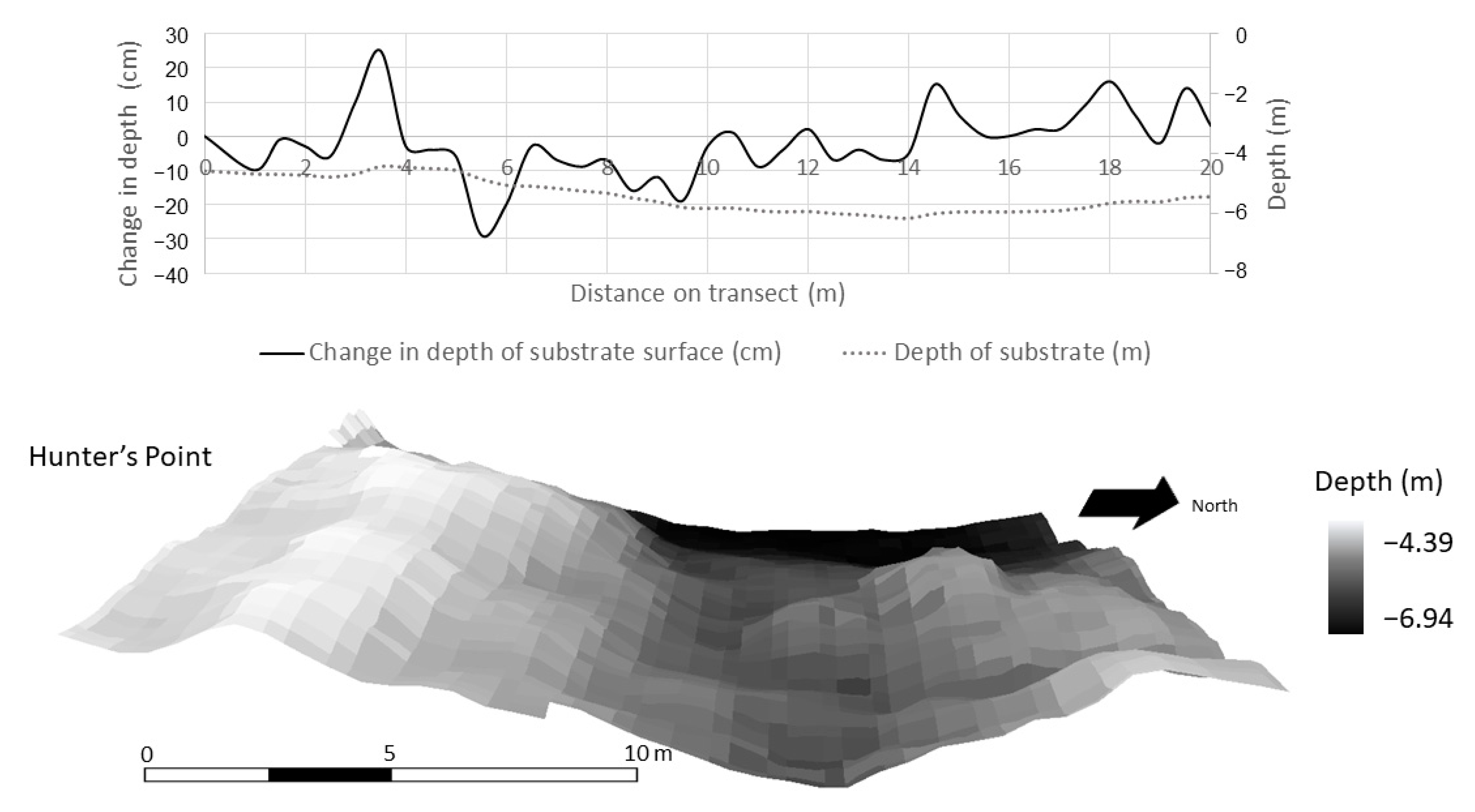
Within a 400 m2 subset at each study site, high-resolution (0.3 m) bathymetry data from the AUV revealed that substrate surface structure was more variable at BP and HP than ML (Figure 8, Figure 9 and Figure 10). This resolution was necessary in the context of the periphyton habitat, where communities respond at a much finer scale than the 4-m resolution bathymetry data. This scale depicts the variability in the texture of the lake bottom as it relates to habitat structure. The change in depth of substrate over a 0.3 m distance averaged 3.88 ± 0.50 cm at BP. At HP, the substrate structure was more than two times more variable and averaged at 7.87 ± 1.10 cm over a 0.3-m distance. The substrate at ML was smooth and did not provide much structure or surface area for periphyton. The average change in the depth of substrate over 0.3 m at ML was 1.76 ± 0.22 cm. Over a 400 m2 area and at a resolution of 0.3 m, substrate surface area averaged 400.74 ± 6.67 m2 at ML, 404.30 ± 2.29 m2 at BP, and 426.2 ± 6.7 m2 at HP (Figure 8, Figure 9 and Figure 10, respectively).
With predicted lake level changes ranging between −0.63 and 0.52 m, the amount of available habitat will change. Based on the bathymetric structure of each site, a 0.63-m drop in lake levels will substantially expand the amount of exposed substrate by as much as 36 m in areas with shallow slopes (<3°) at ML and BP. This exposure equates to a reduction in the available surface area for periphyton habitat by 600 to 3000 m2 per 100 m of shoreline. At HP, with slopes ranging 2 to 9°, a 0.63 m drop in lake levels will expose 426 to 1917 m2 of substrate per 100 m of shoreline. If water levels rise, the surface area of substrate will increase by 150 to 370 m2 per 100 m of shoreline, as the slopes above the lake levels are steeper, and range 8–20°.
4. Discussion
Periphytic diatom community assemblages were different at Brunette Park (BP), Hunter’s Point (HP), and McLain SP (ML). Since physio-chemical parameters were similar at these sites, our study provides evidence that subsurface geology influences periphyton community assemblages in the Keweenaw Peninsula.
Microtopography including substrate size, orientation, and surface irregularities can influence algal biomass and species composition [11,13,15,36,37], because it creates microhabitats that have different resource availability (e.g., colonization area, light), sedimentation efficiency [38], cell adhesion [39], water flow [40], and protection from disturbances such as grazing or scouring [13,36]. Greater surface irregularities are likely to protect small adnate species [13], whereas large, loosely attached species make use of light and nutrients [41]. The orientation of the substrate can alter the water flow (e.g., laminar vs. turbulent), light intensity, and predation of periphyton [15,37,42]. Murdock and Dodds [15] discovered that rougher, more horizontal surfaces collected more algal biomass in a single Kansas stream, and Glasby and Connell [42] found that epibiotic community assemblages differed between horizontal and vertical surfaces in Australian rocky reefs. The physical size of substrata can also influence periphyton communities. Ledger and Hildrew [11] found that total chlorophyll biomass, dry-mass, and density of algal units increased with substrate particle size in an acidic stream in southern England.
Differences in substrate and microtopography at our study sites likely contributed to periphyton community differences. At a fine scale (less than 2 mm), the sand grains of Jacobsville (BP) and Freda sandstone (ML) have greater surface roughness than Copper Harbor Conglomerate (HP) [19]. Souza and Ferragut [16] determined that increasing the surface roughness resulted in decreases in periphyton using stalks and pads, and increases in periphyton using mucilaginous matrices. Our results were not as definitive. BP and ML were characterized by both greater roughness of the substrate particles, but smoother bathymetric structure. At these sites, there were greater amounts of the stalked diatoms, Achnanthidium minutissimum and Gomphonema procerum, whereas the substrate particles at HP were less rough, but the bathymetric structure was more variable. However, HP was characterized by another stalked diatom, Cymbella helvetica. Part of this confusion could be explained by A. minutissimum, which adheres to the substrate using shorter mucilaginous stalks than other stalked diatoms. In addition, Souza and Ferragut [16] determined that an increasing biofilm over the course of their study may have minimized the effect of roughness. Bergey [36] found that small crevices were dominated by A. minutissimum and smooth services by adnate diatoms. Substratum roughness can provide relief from grazing [13] and brushing [15]. Since subsurface geology at HP was less rough and thus provided little refuge, it is not surprising that these microhabitats would facilitate taxa capable of rapid colonization, such as C. helvetica [43]. Variable surface roughness based on geology provided at our three sites in the Keweenaw, could provide the microhabitats required by periphyton with different attachment strategies.
Substrate roughness can be difficult to separate from geology, as they are often correlated. Rock type and geologic formation can cause dissolved minerals to influence periphyton habitat [12]. Conductivity can be influenced by mineral components of the pore fluid [19]. Although Bergey [13] found no difference of algal growth with substratum chemistry, we can only speculate as our measurements for parameters such as electrolytic conductivity, were in the water directly above the benthos. As a result, our study cannot assess the potential chemical influence of geology on periphyton habitat.
All sampling depths included in the current study were from the active wave zone. As a result, in addition to substrate roughness, it is also possible that physical disturbance from wave action is shaping these periphyton communities. Unfortunately, physical disturbance from wave action in lentic habitats remains understudied, as the focus of past research on physical disturbance has been conducted in lotic environments. In a small, geographically proximate, inland lake natural and artificial physical disturbance was investigated [44]. The results of this study from the natural physical disturbance of wave action showed that tightly adhered taxa such as Achnanthidium were present at the highest abundances near shore in the higher disturbance zone, while longer stalked taxa (e.g., Gomphonema) and species that form filaments loosely attached to substrates (e.g., Tabellaria, some Encyonema) increased in presence as disturbance decreased. Similar trends can be seen in the shifting abundances of the species within different study areas (Figure 3). In the present study, the increase in Tabellaria abundance with increasing depth is consistent with Thomas [44] as it is likely washed away from shoreline communities due to wave action, but present in higher abundances at depth as it is able to settle to the bottom undisturbed. The decrease in Achnanthidium minutissimum at ML is also consistent with past results, which showed that adnate attached taxa are outcompeted in low disturbance, deeper sites and are most abundant near shore. The response of Encyonema silesiacum, which lives in tubes of mucilage forming long thin “colonies”, at ML and BP, increasing at depth/lower disturbance fits with this model, but at HP runs counter to this thinking. Gomphonema procerum abundance does not change much at any one site, but is different between sites, so despite its attachment to surfaces with mucilage stalks, it does not seem to be responding to differing levels of disturbance in these systems.
With predicted lake level changes ranging from a −0.63 m drop to an increase in lake levels by +0.52 m [17], the amount of surface area of periphyton habitat will change at each site. Since periphyton assemblages were different at BP, HP and ML, changes in lake levels will likely result in increases in some taxa and decreases in others. For instance, in areas such as ML and BP with shallow slopes ranging <3°, the amount of periphyton habitat will decrease drastically with lake level drops exposing more substrate, but the relative abundance of stalked species such as A. minutissimum will increase and replace species such as Enoyonopsis cesatii, which were more abundant at deeper depths. In areas of Lake Superior with more variable bathymetry, species such as T. flocculosa and E. cesatii will likely increase in relative abundance, whereas A. minutissimum will decrease. Due to steeper bathymetric slopes at HP, the changes in relative abundance of periphyton species will not be as drastic as those at ML and BP, because water level drops will not expose as much substrate at HP. In some areas, a predicted drop in lake levels of 0.63 m may expose 10x as much substrate in shallow sites (ML and BP) than in sites such as HP with steeper bathymetric slopes. Although the relative abundance of species at each site will change with changes in water levels, the composition of communities will likely remain relatively similar, as periphyton diatom assemblages did not substantially differ as a function of depth. More specifically, since the geology of the substratum was similar within the range of depths analyzed in this study, the periphyton at a macro-scale will likely change, but the overall similarity across depths will remain high.
5. Conclusions
If Lake Superior water levels change, the surface area of periphyton habitat will change in the Keweenaw Peninsula to varying degrees based on bathymetry. Although our study does not test the cause-and-effect relationship between subsurface geology and periphytic diatom assemblages, our results provide evidence that differences in microtopography provided by geologic formations in the Keweenaw contribute to differences in periphytic diatom assemblages. As such, if the surface area of geologic formations changes with water levels, periphyton community assemblages will likely change. Since periphyton represent the base of the aquatic food web in Keweenaw, this shift in species composition could have implications for additional species.
Author Contributions
All authors contributed in multiple ways throughout the completion of this project, more specifically: conceptualization, M.M.W.-S., A.L. and E.W.T.; methodology, M.M.W.-S., A.L. and E.W.T.; software and formal analyses, A.L. (spatial analyses and validation), M.M.W.-S. (univariate and multivariate analyses); Investigation, M.M.W.-S. and E.A.; resources, M.M.W.-S., A.L. and E.W.T.; writing—original draft preparation, A.L., M.M.W.-S., E.W.T., E.A.; writing—review and editing, M.M.W.-S., A.L., E.W.T., E.A.; project administration, M.M.W.-S., A.L.; funding acquisition, A.L., M.M.W.-S. All authors have read and agreed to the published version of the manuscript.
Funding
This research received no external funding.
Institutional Review Board Statement
Not applicable.
Informed Consent Statement
Not applicable.
Data Availability Statement
Data presented in this study are available on request from the corresponding author.
Acknowledgments
We wish to thank Grand Valley State University’s Center for Scholarly and Creative Excellence for funding this project. In addition, we thank Jim DeGraff from Michigan Technological University for sharing his geology expertise. His insight greatly improved our manuscript.
Conflicts of Interest
The authors declare no conflict of interest.
References
- Great Lakes Integrated Sciences and Assessments (GLISA). Annual Climate Trends and Impacts Summary for the Great Lakes Basin. Available online: http://glisa.umich.edu/resources/annual-climate-summary (accessed on 23 November 2020).
- Gronewald, A.D.; Hunter, T.S.; Allison, J.; Fry, L.M.; Kompoltowicz, K.A.; Bolinger, R.A.; Pei, L. Project Documentation Report for Great Lakes Seasonal and Inter-Annual Water Supply Forecasting Improvements Project Phase I: Research and Development; NOAA Great Lakes Environmental Research Laboratory, U.S. Army Corps of Engineers Detroit District and the University Corporation for Atmospheric Research: Ann Arbor, MI, USA, 2017.
- United States Army Corps of Engineers. Great Lakes Water Level Data. Available online: https://www.lre.usace.army.mil/Missions/Great-Lakes-Information/Great-Lakes-Information-2/Water-Level-Data/ (accessed on 21 November 2020).
- Nicholls, K.H. Effects of temperature and other factors on summer phosphorus in the inner Bay of Quinte, Lake Ontario: Implications for climate warming. J. Great Lakes Res. 1999, 25, 250–262. [Google Scholar] [CrossRef]
- Smith, A.L.; Hewitt, N.; Klenk, N.; Bazely, D.R.; Yan, N.; Wood, S.; Henriques, I.; MacLellan, J.I.; Lipsig-Mummé, C. Effects of climate change on the distribution of invasive alien species in Canada: A knowledge synthesis of range change projections in a warming world. Environ. Rev. 2012, 20, 1–16. [Google Scholar] [CrossRef]
- Kraemer, B.M.; Anneville, O.; Chandra, S.; Dix, M.; Kuusisto, E.; Livingstone, D.M.; Rimmer, A.; Schladow, S.G.; Silow, E.; Sitoki, L.M.; et al. Morphometry and average temperature affect lake stratification responses to climate change. Geophys. Res. Lett. 2015, 42, 4981–4988. [Google Scholar] [CrossRef] [Green Version]
- Mason, L.A.; Riseng, C.M.; Gronewold, A.D.; Rutherford, E.S.; Wang, J.; Clites, A.; Smith, S.D.P.; McIntyre, P.B. Fine-scale spatial variation in ice cover and surface temperature trends across the surface of the Laurentian Great Lakes. Clim. Chang. 2016, 138, 71–83. [Google Scholar] [CrossRef]
- Lowe, R.L.; Pan, Y. Benthic Algal Communities and Biological Monitors. In Algal Ecology: Freshwater Benthic Ecosystems; Stevenson, R.J., Bothwell, M.L., Lowe, R.L., Eds.; Academic Press: San Diego, CA, USA, 1996; pp. 705–739. [Google Scholar]
- Kingston, J.C.; Lowe, R.L.; Stoermer, E.; Ladewski, T.B. Spatial and temporal distribution of benthic diatoms in northern Lake Michigan. Ecology 1983, 64, 1566. [Google Scholar] [CrossRef]
- Hagy, J.D., III; Houthon, K.A.; Beddick, D.L., Jr.; James, J.B. Quantifying stream periphyton assemblage responses to nutrient amendments with a molecular approach. Freshw. Sci. 2020, 39, 292–308. [Google Scholar] [CrossRef]
- Ledger, M.E.; Hildrew, A.G. Temporal and spatial variation in the epilithic biofilm of an acid stream. Freshw. Biol. 1998, 40, 655–670. [Google Scholar] [CrossRef]
- Sanson, G.; Stolk, R.; Downes, B. A New Method for Characterizing Surface Roughness and Available Space in Biological Systems. Funct. Ecol. 1995, 9, 127–135. [Google Scholar] [CrossRef]
- Bergey, E.A. How protective are refuges? Quantifying algal protection in rock crevices. Freshw. Biol. 2005, 50, 1163–1177. [Google Scholar] [CrossRef]
- Burkholder, J.M. Interactions of benthic algae with their substrata. In Algal Ecology: Freshwater Benthic Ecosystems; Stevenson, R.J., Bothwell, M.L., Lowe, R.L., Eds.; Academic Press: London, UK, 1996; pp. 253–298. [Google Scholar]
- Murdock, J.N.; Dodds, W.K. Linking benthic algal biomass to stream substratum topography 1. J. Phycol. 2007, 43, 449–460. [Google Scholar] [CrossRef]
- Souza, M.L.D.; Ferragut, C. Influence of substratum surface roughness on periphytic algal community structure in a shallow tropical reservoir. Acta Limnologica Brasiliensia 2012, 24, 397–407. [Google Scholar] [CrossRef] [Green Version]
- Great Lakes Environmental Research Lab: Great Lakes Dashboard. Available online: https://www.glerl.noaa.gov/data/dashboard/GLD_HTML5.html (accessed on 21 November 2020).
- Lofgren, B.M.; Hunter, T.S.; Wilbarger, J. Effects of using air temperature as a proxy for potential evapotranspiration in climate change scenarios of Great Lakes basin hydrology. JGLR 2011, 37, 744–752. [Google Scholar] [CrossRef]
- DeGraff, J.; Department of Geological and Mining Engineering Sciences, Michigan Technological Institute, Houghton, MI, USA. Personal communication, 2020.
- Yousef, F.; Shuchman, R.; Sayers, M.; Fahnenstiel, G.; Henareh, A. Water clarity of the Upper Great Lakes: Tracking changes between 1998–2012. J. Great Lakes Res. 2017, 43, 239–247. [Google Scholar] [CrossRef]
- Stevenson, R.J.; Bahls, L.L. Periphyton Protocols. In Rapid Bioassessment Protocols for Use in Wadeable Streams and Rivers: Periphyton, Benthic Macroinvertebrates, and Fish, 2nd ed.; Barbour, M.T., Gerritsen, J., Snyder, B.D., Stribling, J.B., Eds.; U.S. Environmental Protection Agency: Washington, DC, USA, 1999. [Google Scholar]
- Carr, J.M.; Hergenrader, G.L.; Troelstrup, N.H., Jr. A simple, inexpensive method for cleaning diatoms. Trans. Am. Microsc. Soc. 1986, 105, 152–157. [Google Scholar] [CrossRef]
- Krammer, K.; Lange-Bertalot, H. Bacillariophyceae. 1 Teil: Naviculaceae. In Süsswasserflora von Mitteleuropa 1986, Band 2/1; Ettl, H., Gerloff, J., Heynig, H., Mollenhauer, D., Eds.; Gustav Fisher Verlag: Jena, Germany, 1986; p. 876. [Google Scholar]
- Krammer, K.; Lange-Bertalot, H. Bacillariophyceae, 2 Teil: Bacillariaceae. Epithemiaceae, Surirellaceae. In Süsswasserflora von Mitteleuropa; IEttl, H., Gerloff, J., Heynig, H., Mollenhauer, D., Eds.; Gustav Fisher Verlag: Jena, Germany, 1988; Volume 2, pp. 1–596. [Google Scholar]
- Krammer, K.; Lange-Bertalot, H. Bacillariophyceae, 3 Teil: Centrales, Fragilariaceae, Eunotiaceae. In Süsswasserflora von Mitteleuropa; Ettl, H., Gerloff, J., Heynig, H., Mollenhauer, D., Eds.; Gustav Fisher Verlag: Jena, Germany, 1991; Volume 2, pp. 1–576. [Google Scholar]
- Krammer, K.; Lange-Bertalot, H. Bacillariophyceae, 4 Teil: Achnanthaceae, Kritische Erganzungen zu Navicula (Lineolatae) und Gomphonema, Gesamtliteraturverzeichnis Teil 1–4. In Süsswasserflora von Mitteleuropa; Ettl, H., Gerloff, J., Heynig, H., Mollenhauer, D., Eds.; Gustav Fisher Verlag: Jena, Germany, 1991; Volume 2, pp. 1–437. [Google Scholar]
- Diatoms of North America. Available online: https://diatoms.org/ (accessed on 20 December 2020).
- R Core Team. R: A Language and Environment for Statistical Computing; R Foundation for Statistical Computing: Vienna, Austria, 2017; Available online: https://www.R-project.org/ (accessed on 21 November 2020).
- Fox, J.; Weisberg, S. An {R} Companion to Applied Regression, 2nd ed.; Sage: Thousand Oaks, CA, USA, 2011; Available online: http://socserv.socsci.mcmaster.ca/jfox/Books/Companion (accessed on 21 November 2020).
- Venables, W.N.; Ripley, B.D. Modern Applied Statistics with S, 4th ed.; Springer: New York, NY, USA, 2002. [Google Scholar]
- Oksanen, J.; Blanchet, F.G.; Friendly, M.; Kindt, R.; Legendre, P.; McGlinn, D.; Minchin, P.R.; O’Hara, R.B.; Simpson, G.L.; Solymos, P.; et al. Vegan: Community Ecology Package. R Package 2017, Version 2.4-3. Available online: https://CRAN.R-project.org/package=vegan (accessed on 21 November 2020).
- Environmental Systems Research Institute (ESRI). ArcGIS v 10.4.1; Redlands, CA, USA, 2016. Available online: https://www.esri.com/en-us/home (accessed on 21 November 2020).
- National Oceanic and Atmospheric Association (NOAA). 2019 USACE NCMP Topobathy Lidar DEM: Lake Superior (MI). Available online: https://coast.noaa.gov/dataviewer/#/lidar/search/-9867867.477559684,5977452.048929067,-9755046.423810763,6024384.384296166/details/9185 (accessed on 21 November 2020).
- Angel, J.R.; Kunkel, K.E. The response of Great Lakes water levels to future climate scenarios with an emphasis on Lake Michigan-Huron. J. Great Lakes Res. 2010, 36, 51–58. [Google Scholar] [CrossRef]
- Hayhoe, K.; VanDorn, J.; Croley II, T.; Schlegel, N.; Wuebbles, D. Regional climate change projections for Chicao and the US Great Lakes. J. Great Lakes Res. 2010, 36, 7–21. [Google Scholar] [CrossRef]
- Bergey, E.A. Crevices as refugia for stream diatoms: Effect of crevice size on abraded substrates. Limnol. Oceanogr. 1999, 44, 1522–1529. [Google Scholar] [CrossRef]
- Kralj, K.; Plenković-Moraj, A.; Gligora, M.; Primc-Habdija, B.; Šipoš, L. Structure of periphytic community on artificial substrata: Influence of depth, slide orientation and colonization time in karstic Lake Visovačko, Croatia. Hydrobiologia 2006, 560, 249–258. [Google Scholar] [CrossRef]
- Johnson, L.E. Enhanced settlement on microtopographical high points by the intertidal red alga Halosaccion glandiforme. Limnol. Oceanogr. 1994, 39, 1893–1902. [Google Scholar] [CrossRef]
- Sekar, R.; Venugopalan, V.P.; Satpathy, K.K.; Nair, K.V.K.; Rao, V.N.R. Laboratory Studies on Adhesion of Microalgae to Hard Substrates. In Asian Pacific Phycology in the 21st Century: Prospects and Challenges; Springer: Dordrecht, The Netherlands, 2004; pp. 109–116. [Google Scholar]
- DeNicola, D.M.; McIntire, C.D. Effects of substrate relief on the distribution of periphyton in laboratory streams, i. hydrology 1. J. Phycol. 1990, 26, 624–633. [Google Scholar] [CrossRef]
- Biggs, B.J.F.; Thomsen, H.A. Disturbance of stream periphyton by perturbations in shear stress: Time to structural failure and differences in community resistance. J. Phycol. 1995, 31, 233–241. [Google Scholar] [CrossRef]
- Glasby, T.M.; Connell, S.D. Orientation and position of substrata have large effects on epibiotic assemblages. Mar. Ecol. Prog. Series 2001, 214, 127–135. [Google Scholar] [CrossRef]
- Steinman, A.D. Effects of Grazers on Freshwater Benthic Algae. In Algal Ecology: Freshwater Benthic Ecosystems; Stevenson, R.J., Bothwell, M.L., Lowe, R.L., Eds.; Academic Press: San Diego, CA, USA, 1996; pp. 341–373. [Google Scholar]
- Thomas, E.W. The Role of Wave Disturbance on Lentic, Benthic Algal Community Structure and Diversity. Master’ Thesis, Bowling Green State University, Bowling Green, OH, USA, August 2007. [Google Scholar]
Figure 1.
Geology of the Keweenaw Peninsula (Keweenaw Co., MI, USA) and project sample sites: McLain State Park, Hunter’s Point Park and Brunette Park.
Figure 1.
Geology of the Keweenaw Peninsula (Keweenaw Co., MI, USA) and project sample sites: McLain State Park, Hunter’s Point Park and Brunette Park.

Figure 2.
Process of bathymetric analysis of Lake Superior at three study sites in the Keweenaw Peninsula, Michigan. Topo bathymetry data (4 m) was used to characterize the general structure of the lake bottom at each study site, Brunette Park, Hunter’s Point and McLain State Park (left). At each study site, an autonomous underwater vehicle (AUV) was pre-programmed to collect multibeam XYZ data, which was used to create high-resolution (0.3 m) maps of microtopography at each study site. Three 400 m2 plots were established to quantify the structure of surface irregularities of the substrate for periphyton habitat (right).

Figure 3.
Ordination following non-metric multidimensional scaling of Bray-Curtis similarities of periphytic diatom communities determined at various depths (0–2 m) at Brunette Park (n = 9), Hunter’s Point (n = 5) and McLain State Park (n = 5). Note that although nine samples were analyzed at each site, not all samples contained periphyton, especially in the active wave zone, z = 0 m. Stress = 12.84; ellipses per site represent the 95% confidence interval of the site centroid. Post-hoc Adonis revealed that periphyton communities were significantly different among sites (p < 0.05).

Figure 4.
Relative abundances of periphytic diatoms identified using similarity of percentages (SIMPER) as contributing greater than 50% of differences between sites (BP—Brunette Park, HP—Hunter’s Point, ML—McLain State Park). Letters above site bars indicate significance (p < 0.05) following post-hoc, pairwise Adonis with Holm’s adjustment.

Figure 5.
Average bathymetric profile of three 300-m transects (top), and area bathymetry (4-m resolution) of Lake Superior (bottom) at Brunette Park.
Figure 5.
Average bathymetric profile of three 300-m transects (top), and area bathymetry (4-m resolution) of Lake Superior (bottom) at Brunette Park.

Figure 6.
Average bathymetric profile of three 300-m transects (top), and area bathymetry (4-m resolution) of Lake Superior (bottom) at McLain State Park.
Figure 6.
Average bathymetric profile of three 300-m transects (top), and area bathymetry (4-m resolution) of Lake Superior (bottom) at McLain State Park.

Figure 7.
Average bathymetric profile of three 300-m transects (top), and area bathymetry (4-m resolution) of Lake Superior (bottom) at Hunter’s Point park.
Figure 7.
Average bathymetric profile of three 300-m transects (top), and area bathymetry (4-m resolution) of Lake Superior (bottom) at Hunter’s Point park.

Figure 8.
High resolution bathymetry (0.3 m) collected by an autonomous underwater vehicle in Lake Superior in a randomly selected 20 m × 20 m plot at Brunette Park. Depth profile (top) and area (bottom) documenting the microtopography of periphyton habitat.
Figure 8.
High resolution bathymetry (0.3 m) collected by an autonomous underwater vehicle in Lake Superior in a randomly selected 20 m × 20 m plot at Brunette Park. Depth profile (top) and area (bottom) documenting the microtopography of periphyton habitat.

Figure 9.
High resolution bathymetry (0.3 m) collected by an autonomous underwater vehicle in Lake Superior in a randomly selected 20 m × 20 m plot at McLain State Park. Depth profile (top) and area (bottom) documenting microtopography of periphyton habitat.
Figure 9.
High resolution bathymetry (0.3 m) collected by an autonomous underwater vehicle in Lake Superior in a randomly selected 20 m × 20 m plot at McLain State Park. Depth profile (top) and area (bottom) documenting microtopography of periphyton habitat.

Figure 10.
High resolution bathymetry (0.3 m) collected by an autonomous underwater vehicle in Lake Superior in a randomly selected 20 m × 20 m plot at Hunter’s Point. Depth profile (top) and area (bottom) documenting microtopography of periphyton habitat.
Figure 10.
High resolution bathymetry (0.3 m) collected by an autonomous underwater vehicle in Lake Superior in a randomly selected 20 m × 20 m plot at Hunter’s Point. Depth profile (top) and area (bottom) documenting microtopography of periphyton habitat.


Table 1.
Historic and future Lake Superior water levels (m) along with the water level of the current study (sample collection at z = 0) [17] for comparison.
Table 1.
Historic and future Lake Superior water levels (m) along with the water level of the current study (sample collection at z = 0) [17] for comparison.
| Minimum (m) | Maximum (m) | Reference | |
|---|---|---|---|
| Historic Data (1918–2020) | 182.72 | 183.91 | Great Lakes Dashboard [17] |
| Current Study (2019) | 183.86 | ||
| Future Projections (2068–2105) | 182.42 | 183.74 | Lofgren et al. [18] |
| 183.22 | 183.47 | Angel et al. [34] | |
| 183.24 | 183.27 | Hayhoe et al. [35] |
Table 2.
Mean nitrate, total phosphorus, temperature, dissolved oxygen, and conductivity with standard error and number of observations in parentheses by site (BP—Brunette Park, HP—Hunter’s Point, ML—McLain State Park) and depth (0–2 m).
Table 2.
Mean nitrate, total phosphorus, temperature, dissolved oxygen, and conductivity with standard error and number of observations in parentheses by site (BP—Brunette Park, HP—Hunter’s Point, ML—McLain State Park) and depth (0–2 m).
| Site/ Depth (m) | Nitrate (mg L−1) | Total Phosphorus (ug L−1) | Temperature (C) | Dissolved Oxygen (mg L−1) | Conductivity (μs cm−1) |
|---|---|---|---|---|---|
| BP | 0.33 ± 0.00 (9) | 52.89 ± 3.94 (9) | 19.78 ± 0.27 (9) | 11.59 ± 0.40 (9) | 88.02 ± 0.38 (9) |
| 0 | 0.32 ± 0.01 (3) | 50.67 ± 2.60 (3) | 20.57 ± 0.18 (3) | 10.50 ± 0.14 (3) | 88.67 ± 0.78 (3) |
| 1 | 0.33 ± 0.01 (3) | 57.33 ± 6.89 (3) | 19.30 ± 0.61 (3) | 11.72 ± 0.56 (3) | 87.97 ± 0.80 (3) |
| 2 | 0.33 ± 0.00 (3) | 50.67 ± 10.84 (3) | 19.47 ± 0.09 (3) | 12.54 ± 0.70 (3) | 87.43 ± 0.32 (3) |
| HP | 0.33 ± 0.01 (9) | 50.67 ± 3.84 (9) | 21.30 ± 0.14 (9) | 10.17 ± 0.25 (9) | 91.51 ± 0.22 (3) |
| 0 | 0.35 ± 0.01 (3) | 55.00 ± 7.55 (3) | 21.63 ± 0.30 (3) | 9.22 ± 0.14 (3) | 90.97 ± 0.29 (3) |
| 1 | 0.31 ± 0.02 (3) | 46.00 ± 8.89 (3) | 21.30 ± 0.15 (3) | 10.83 ± 0.26 (3) | 92.23 ± 0.23 (3) |
| 2 | 0.32 ± 0.00 (3) | 51.00 ± 4.58 (3) | 20.97 ± 0.09 (3) | 10.47 ± 0.09 (3) | 91.33 ± 0.15 (3) |
| ML | 0.32 ± 0.00 (9) | 58.11 ± 5.09 (9) | 20.88 ± 0.61 (9) | 9.88 ± 0.13 (9) | 93.42 ± 1.73 (3) |
| 0 | 0.31 ± 0.00 (3) | 65.33 ± 8.35 (3) | 23.30 ± 0.11 (3) | 9.61 ± 0.06 (3) | 97.03 ± 4.60 (3) |
| 1 | 0.32 ± 0.00 (3) | 49.67 ± 3.48 (3) | 19.90 ± 0.11 (3) | 9.77 ± 0.06 (3) | 93.07 ± 0.98 (3) |
| 2 | 0.32 ± 0.01 (3) | 59.33 ± 12.91 (3) | 19.43 ± 0.12 (3) | 10.25 ± 0.28 (3) | 89.90 ± 0.23 (3) |
Publisher’s Note: MDPI stays neutral with regard to jurisdictional claims in published maps and institutional affiliations. |
© 2021 by the authors. Licensee MDPI, Basel, Switzerland. This article is an open access article distributed under the terms and conditions of the Creative Commons Attribution (CC BY) license (http://creativecommons.org/licenses/by/4.0/).
Share and Cite
MDPI and ACS Style
Woller-Skar, M.M.; Locher, A.; Audia, E.; Thomas, E.W. Changing Water Levels in Lake Superior, MI (USA) Impact Periphytic Diatom Assemblages in the Keweenaw Peninsula. Water 2021, 13, 253. https://doi.org/10.3390/w13030253
AMA Style
Woller-Skar MM, Locher A, Audia E, Thomas EW. Changing Water Levels in Lake Superior, MI (USA) Impact Periphytic Diatom Assemblages in the Keweenaw Peninsula. Water. 2021; 13(3):253. https://doi.org/10.3390/w13030253
Chicago/Turabian StyleWoller-Skar, M. Megan, Alexandra Locher, Ellen Audia, and Evan W. Thomas. 2021. "Changing Water Levels in Lake Superior, MI (USA) Impact Periphytic Diatom Assemblages in the Keweenaw Peninsula" Water 13, no. 3: 253. https://doi.org/10.3390/w13030253
Note that from the first issue of 2016, this journal uses article numbers instead of page numbers. See further details here.