
Multi-Scale Target-Specified Sub-Model Approach for Fast Large-Scale High-Resolution 2D Urban Flood Modelling


1
Department of Geoscience and Natural Resource Management, University of Copenhagen, Rolighedsvej 23, 1958 Frederiksberg C, Denmark
2
Krüger A/S, Søborg, 2860 Hovedstaden, Denmark
*
Author to whom correspondence should be addressed.
Water 2021, 13(3), 259; https://doi.org/10.3390/w13030259
Submission received: 25 November 2020
/
Revised: 16 January 2021
/
Accepted: 18 January 2021
/
Published: 21 January 2021
(This article belongs to the Special Issue Urban Water Management and Urban Flooding)
Abstract
:The accuracy of two-dimensional hydrodynamic models (2D models) is improved when high-resolution Digital Elevation Models (DEMs) are used. However, the entailed high spatial discretisation results in excessive computational expenses, thus prohibiting their implementation in real-time forecasting especially at a large scale. This paper presents a sub-model approach that adapts 1D static models to tailor high-resolution 2D model grids relevant to specified targets, such that the tailor-made 2D hydrodynamic sub-models yield fast processing without significant loss of accuracy via a GIS-based multi-scale simulation framework. To validate the proposed approach, model experiments were first designed to separately test the impact of two outcomes (i.e., the reduced computational domains and the optimised boundary conditions) towards final 2D prediction results. Then, the robustness of the sub-model approach was evaluated by selecting four focus areas with distinct catchment terrain morphologies as well as distinct rainfall return periods of 1–100 years. The sub-model approach resulted in a 45–553 times faster processing with a 99% reduction in the number of computational cells for all four cases; the goodness of fit regarding predicted flood extents was above 0.88 of F2, flood depths yield Root Mean Square Errors (RMSE) below 1.5 cm and the discrepancies of u- and v-directional velocities at selected points were less than 0.015 ms−1. As such, this approach reduces the 2D models’ computing expenses significantly, thus paving the way for large-scale high-resolution 2D real-time forecasting.
1. Introduction
Urban floods pose escalating threats to human settlements in times of continued urbanisation and climate change [1]. To mitigate the flood risks and the related consequences, a flood forecasting system that complies with two criteria: (i) accurate spatial and temporal flood predictions and (ii) sufficient lead time between rainfall predictions and flood predictions, is considered as a prerequisite to provide precise early warnings for decision-makers. Therefore, to identify an accurate and timely urban flood model to configure such a system, we review two types of models: (i) 2D hydrodynamic models (Section 1.1) and (ii) 1D static models (Section 1.2). After summarising the strengths and potentials for the two models, the scientific innovation of the proposed approach is outlined by identifying a 1D/2D complementary solution maximising the potentials of two models while minimizing their limitations (Section 1.3).
1.1. 2D Hydrodynamic Models (2D Models)
By enabling more realistic 2D dynamic flows across regular grids, 2D models are advocated as a preferential approach for urban flood simulations [2,3,4,5,6]. However, 2D models tend to be computationally expensive. When numerical solvers (implicit/explicit solvers) are executed in a high spatial discretisation based on a fine grid, to stabilise the models, the optimum time steps must be decreased accordingly, which boost processing time considerably. Although applying a coarse grid is considered a straightforward way to reduce computing time, it turns out that the extra details inherent in high-resolution DEMs can benefit simulation accuracy substantially [7,8,9]. Particularly when micro-topography dominates the direction of flood propagation, grid coarsening may smear critical elevation information resulting in imprecise inundation distributions [10,11]. Recently, the occurrence of decimetric DEMs allows for the inclusion of more detailed micro-topographies in urban flood models, which initiates a new high-resolution simulation era. However, due to the prohibitive processing time, high-resolution applications have been limited to small scale modelling only [10,12]. For the same reason, the use of high-resolution grids in real-time forecasts (nowcasting) is impractical. Consequently, applying high-resolution DEMs to large-scale modelling and real-time forecasts remains challenging.
To improve the 2D models’ computational efficiency, four speed-up approaches may be employed: (i) parallelization technology taking advantage of Graphics Processing Units (GPUs), multi-core Central Processing Units (MCs), remotely distributed computers and cloud computing such as JFLOW-GPU [13], OpenMP [14], MPI libraries [15], FloodMap-Paraller model [16] and CityCAT [17]; (ii) a simplified hydrodynamic model approach that solves simplified governing equations, whereby reasonable flood extents and depths can be yielded quickly although the momentum conservation is less emphasized, e.g., inertial LISFLOOD-FP [18] and Quasi 2D [19]; (iii) a coarse-grid approach, where computational time is reduced by increasing the grid size [8]; to compensate for loss of accuracy due to smearing of details, especially around buildings, various improvements have been introduced, including sub-grid treatment [20,21,22], the multi-cell approach [23], the multi-layered approach [24] and the porosity parameter approach [25,26,27,28]; and (iv) the Cellular Automata (CA) approach, where a universal transition rule is coded for spatial discretization in the simulation, thus achieving a reduced-complexity procedure in 2D models [29,30,31,32]. Whereas these technologies may reduce computational costs to some extent, new fast-approaching remote sensing technologies delivering enhanced data accuracy in tremendous volumes are even more difficult for them to handle [10,12,33,34,35,36,37,38,39,40,41,42]. Especially, the use of a high-resolution modelling grid is the precondition to explicitly include all detailed spatial representations of datasets into 2D simulations. Thus, the computational efficiency of 2D models remains a challenge in the high-resolution data context.
1.2. 1D Static Models (Fast-Inundation Models)
Due to the fast processing speed, 1D models have been widely implemented in engineering practices for decades [43,44,45,46,47,48]. With the simulation time in seconds, 1D fast-inundation models have been drawn increasing attention. Noteworthy examples include RFIM [49,50,51], RFSM [52,53,54], ISIS-FAST [55], FCDC [56], GUFIM [57], SCALGO [58], USISM [59] and Arc-Malstrøm [60], CA-ffé [61] and Safer_RAIN [62]. A conception of “hydrostatic condition” [52], also known as the “flat water assumption” [63] is commonly embedded as the underlying algorithm in these models. With mass conservation as the only governing law and disregarding temporal evolution, the fast-inundation models present a filling/spilling process within the predefined flow patterns thus resulting in rapid predictions. In this piece of research, we name the process “1D static flow”. This type of model is divided into two types [59]: one is used for point-source triggered floodings caused by dam breaching and riverbank overflow (RFIM, RFSM, ISIS-FAST, FCDC, CA-ffé); the other (non-point source models) is more directly relevant to stormwater-inundations in urban areas (GUFIM, USISM, Arc-Malstrøm, Safer_RAIN). By using 1D static flows instead of 2D hydrodynamic flows the fast inundation models gain computational efficiency substantially, and thus a fast-processing speed is obtained particularly when dealing with large-scale high-resolution DEMs. However, there are two notable drawbacks: Firstly, due to their intrinsic neglect of time evolution, they cannot reproduce flow dynamics (i.e., hydrographs), and peaks may be miss-captured in such static simulations; Secondly, they do not account for the conservation of momentum and, therefore, cannot provide flow velocities, which is essential to flood risk assessments.
1.3. Hypothesis and Research Objectives
In combination with Geographic Information System (GIS), 1D models can be a powerful tool for the large-scale urban flood modelling [3]. So, the idea is to use 1D models to rapidly identify a coarse 1D flow condition at a large scale, and then based on the 1D results, those high-resolution 2D model grids that do not pose a flood risk to specified targets, i.e., irrelevant grids, are to be eliminated. Ultimately, detailed 2D hydrodynamic models using the tailored model girds can be executed cost-efficiently at a local catchment scale. In addition, given the specific modelling task, the selected models should be tailored by deliberately ignoring the incidental modelling complexities [64]. Here, to pursue the fastest processing speed, a 1D static model (i.e., Arc-Malstrøm) using the simplest “filling/spilling routine” was selected and thus the other 1D hydrodynamic models reflecting the temporal evolution were omitted deliberately. Meanwhile, to pursue the highest accuracy in flow dynamics, a full 2D model (i.e., MIKE FLOOD) was selected, and thus the other fast 2D models using numeric approximations were omitted deliberately. In this way, the combination would avoid the prohibitive processing time in full 2D models while compensating for the deficiencies in 1D static models, therefore achieving a 1D/2D complementary approach [65]. To authors’ literature knowledge, this is the first time that 1D and 2D models are utilised together via a GIS-based multi-scale simulation framework.
This paper presents a sub-model approach that adapts the 1D static model for tailoring the 2D model grids based on specified targets, thus achieving fast large-scale high-resolution 2D hydrodynamic modelling without significant loss of the accuracies. To investigate the influence of the domain reductions, the MIKE FLOOD predictions based on the sub-model domain were benchmarked against the ones for the full domain, and further compared to the one defined from municipality borders. Meanwhile, to investigate the validity of the suggested boundary conditions, the discrepancies of optimal boundary condition were compared to the ones of uniform closed-/open-boundary conditions. Finally, to prove robustness, performances of four sub-models in the context of different terrain morphologies as well as different rainfall return periods were benchmarked and compared.
2. Methodology
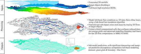
The sub-model approach consists of three modules (Modules I–III, as illustrated in Figure 1 and Appendix A). Module I extracts the 1D network from the DEMs and enables a fast-inundation simulation considering the spatial-varying rainfall. Modules II performs the upstream tracing operation and identifies the sub-impact zones relevant to specified targets. Module III extracts the critical computational cells based on identified sub-impact zones and configures the reduced domain and the optimised boundary condition for the full 2D hydrodynamic modelling. The general procedure is programmed and wrapped up within the ArcGIS Desktop ver. 10.6’s Python programming interface (ArcPy).
2.1. 1D Network Generation and Fast-Inundation Modelling (Module I)
To extract the 1D surface network from the large-scale high-resolution DEMs, we used the GIS-based method developed by [60]. The 1D network includes four hydro-objects: blue spots (sinks), their sub-impact zones (catchments), their pour points, and stream links. “Blue spots” refers to all surface depressions [66]. “Sub-impact zones” describes the blue spots’ upstream catchments based on so-called “8N approach” [67,68,69]. “Pour points” denotes the overflow positions along the blue spots’ rims. “Stream links” describes the topological connectivity between blue spots, i.e., flow paths. For the detailed GIS workflow, please refer to [60]. In addition, to quickly estimate a coarse flood volume distribution (i.e., Boolean flow conditions, spill-over/non-spill-over) across the basin-wise 1D network, we developed a link-based fast-inundation algorithm (Figure 2a).
The suggested algorithm uses stream links as computational objects. Therefore, all information related to sink features (points), i.e., Csink, Vrunoff, Vreceived, Vspilled and Vremaining, is joined onto their intersected stream links (edges). This allows for the subsequent fast-inundation calculation to be exclusively based on one stream link feature class’ attribute table (see Figure 3c). The Shreve stream order [70] is used to determine the correct computational order of stream links and the convergence order of excess flows. By governing the conservation of mass balance within each stream link, flood volumes are computed according to two flow conditions:
If , then Flow condition I is computed as below:
Else , then Flow condition II is computed as below:
Notably, to account for the spatial-varying rainfall, Vrunoff is computed as below:
where Csink is the sink’s capacity, and Vrunoff is runoff volume generated from the sink’s catchment. Rcellsize is the cell size of the 2D rainfall (distributed dynamic rainfall) that has the commensurate cell size of DEMs; Ai is the total rainfall depth contained by cell i in the total rainfall raster (distributed static rainfall) that is aggregated from the 2D rainfall, and n is the total number of rainfall cells within each sink’s catchment. Vspilled represents excess volumes once the spill-over level is reached, Vremaining is the actual volume retained locally, and Vreceived represents the converged flow volumes received from upstream connecting links. Notably, the hydrological losses (i.e., evaporation and infiltration) and the presence of underground drainage systems can be estimated as subtracted volumes either from the corresponding sink capacity (i.e., Csink) or the total rainfall.
After enabling this algorithm, a stream link feature class incorporating geometric features and their associated attribute table is produced (Figure 3a,c). In addition to the computed results of Vspilled and Vremaining, topological connectivity identifying the next downstream stream link is also self-established in the same table (upstream & downstream sink ID, see Figure 3c), which is now ready for the upstream tracing operation as illustrated in Figure 3b. In contrast to the method reported by [60], this new algorithm self-establishes a data structure configuring all information within one table for the flooding computation as well as the upstream tracing operation, thus leaving off the previous ArcGIS’s geometric network environment. In addition, the use of Shreve stream order has effectively issued the challenge of the computing order confusions due to the occurrence of infinite flow loops in the 1D network. Both factors facilitate the automation and wrap-up of all modules in the Python programming environment.
2.2. Targets-Based Upstream Tracing Operation (Module II)
To identify the relevant sub-impact zones, an algorithm is programmed to perform an upstream tracing operation based on the stream link feature class. As illustrated in Figure 2b, when introducing the target objects among urban infrastructures (e.g., buildings, parks and roads) as input variables, the intersecting stream link features are first selected (i.e., S8 as it intersects with Sink I) representing local inundations as well as their associated inflow paths. Here, although spill-overs—due to the possible high-momentum flows—may impact all the neighbourhood flow conditions, their significant volumes would follow the preferential paths indicated by stream links, thus affecting the downstream flow conditions primarily. Meanwhile, a sink could receive multiple inflows. To fully expose multiple inflow paths, the procedure continuously matches all stream links by indexing the current upstream sink ID until all the upstream stream links being identical downstream sink ID were included (Figure 3c). More importantly, to reflect the actual flow continuity beyond flow paths (simply indicating flow directions), flood volumes along the stream links are considered by conserving the mass balance during the whole tracing procedure. Here, based on Vspilled, we introduce a Boolean flow condition property (spill-over/non-spill-over, see Figure 3c) as a search termination criterion. So, stream links associated with non-spilt-over sinks (i.e., tracing-brake features) are excluded from the search list, which results in optimal stream links (i.e., S8-S6-S3-S1 or S8-S6-S4). In case of heavy rainfall, the tracing distance would increase with more involved stream links due to the more densified spilling configurations and vice versa (Figure 4). This thereby avoids a substantial risk of tracing all connected flow paths basin-wise, such as Arc-Malstrøm’s upstream tracing function and ArcGIS’ Watershed tool. Finally, since these identified stream links represent all main flows related to specified inundation modelling, their intersected sub-impact zones would suggest suitable modelling areas (domains) covering relevant runoff generations (sheet-flow) as well as flood propagations (channel-flow).
2.3. Tailor-Made 2D Sub-Model Tailoring and Modelling (Module III)
Urban flow is usually characterised by numerous transitions of supercritical flows and numerical shocks [71]. Full 2D models are considered as best candidates to expose the complicated flow dynamics. Thus, MIKE FLOOD’s rectangular cell solver, which solves alternating direction implicit schemes on inertia wave equations (ADI), is used in this module to obtain hydrodynamic 2D flow predictions [72]. More importantly, by accounting for identified sub-impact zones, critical computational grid-cells (dark orange cells) intersecting them are extracted from the high-resolution DEM’s grid. Thus, a reduced modelling grid extent is identified simultaneously, resulting in efficient computational costs for MIKE FLOOD’s 2D simulations, see Figure 5a,b. Besides, the suggested 1D flow patterns (blue edges) define that runoffs generated within the identified sub-impact zones must exit at downstream terminal pour points (i.e., Sink I’s pour point), only. To be consistent with these described 1D flow conditions, the irrelevant grid-cells (light orange cells) within the reduced modelling grid extent should be assigned the Nodata value to prevent outwards 2D flow leakages along upstream edges. 2D weirs should be established by pulling up the terminal pour point’s surrounding elevation values (marked ↓ in Figure 5b) to the spilling level, while sufficient retention volumes >Vspilled should be accommodated to the downstream side of the 2D weirs by decreasing the associated grid-cell elevations (marked × in Figure 5b). With establishing the closed boundary conditions along the upstream edges and the open-boundary conditions at all the terminal pour point positions, we define such a boundary condition set-up as the optimised boundary conditions (the red outline). Notably, for the grid-cells intersecting the internal subtracted areas or buildings, their elevation values should be substituted by a specified value (e.g., 100). As such, the computational domain excluding Nodata value as well as the specified value defines the final computational domain for 2D models thus configuring the reduced domains (dark orange cells) for the sub-model approach. Based on the reduced domain and the optimised boundary conditions determined above, additional complexities (e.g., hydrological losses, distributed roughness surface values, impervious surface types, subsurface flows and hydraulic behaviours concerning rooftops) may be involved subsequently at the local catchment scale. Thus, this GIS-based method ultimately produces tailor-made sub-models providing fast 2D flow predictions.
2.4. Model Experiments
The sub-model approach suggests two outcomes: (i) reduced computational domains and (ii) optimised boundary conditions. To clarify the individual effect, their validities were investigated separately as two-folds: On one hand, the suggested domains can lead to fast 2D predictions in MIKE FLOOD. Yet, their prediction accuracy may be affected as well. To quantify the influence of domain reductions, tests using consistent boundary conditions were conducted to validate this method against benchmark results, and the other domain reduction approach (Municipality domain approach, Section 2.4.1) was used for comparison purposes. On the other hand, optimised boundary conditions may lead to prediction discrepancies along the boundary areas. To evaluate the influence of the various boundary conditions adopted, tests (Section 2.4.2) using the consistent domain were conducted to compare benchmarking discrepancies in different boundary conditions. Furthermore, according to [73], different terrain morphology may impact overland flow patterns significantly, tests (Section 2.4.3) were carried out on different catchments (within the Greve basin described in Section 3.1) under different associated regional rainfalls (Section 3.3) to validate the robustness of the sub-model approach.
2.4.1. Domain Reduction Tests (Sub-Model Approach vs. Municipality Domain Approach)
We identified the full-basin domain approach, where the entire drainage basin area has flow directions pointing towards the outlet (i.e., ArcGIS’ Basin/Watershed tool). Further, this approach converts the whole area into the full 2D domain in MIKE FLOOD. As we enable 2D dynamic flows at the full-basin domain, this approach reproduces the most accurate flow dynamics thus taken as the benchmark solution. Yet, without having any specified targets, this approach reflects general modelling targets. In contrast, taking the buildings within focus area A as the specific target objects (Map A, Figure 6), we identified two different reduced domains following two approaches: (i) the sub-model approach, where the sub-model domain was delineated as the suggested approach; (ii) the municipality domain approach, where a reduced domain was delineated simply based on municipality borders enveloping all target objects.
To ensure the consistent starting point for comparisons, the same inputs—i.e., DEMs Section 3.2 and Rainfall Section 3.3—were used for the three approaches. Yet, due to the different domains determined from the different approaches, the two inputs for the sub-model approach and the municipality domain approach were tailored by having a mask operation (e.g., ArcGIS’ Extract by Mask tool) based on their suggested domain, respectively. Finally, the predictions of the sub-model approach and the municipality domain approach were both validated against the benchmark solution within the same extents of the masks, and discrepancies of the two approaches were further compared regarding flood extents, flood depths, internal points’ hydrographs and computational efficiencies. In this test, to exclude the influence of the inconsistent boundary conditions, uniform closed-boundary conditions were adopted for all three approaches (the test results based on uniform open-boundary conditions are provided in Appendix A).
2.4.2. Boundary Condition Comparison Tests (Optimised Boundary Conditions vs. Uniform Closed-Boundary Conditions vs. Uniform Open-Boundary Conditions)
We identified the optimised boundary conditions as suggested by the sub-model approach. With the same sub-model domain, the simulations based on uniform closed-boundary conditions and the uniform open-boundary conditions were carried out for comparison purposes. Like in Section 2.4.1, the same rainfall input was used for the three approaches. All these results were validated against the benchmark solution within the same extent of the sub-model domain respectively, and their discrepancies were compared regarding flood extents and flood depths. Finally, the internal points that illustrated significant discrepancies in hydrographs (Section 2.4.1) were investigated further.
2.4.3. General Applicability Tests (Sub-Model A vs. B vs. C vs. D)
We selected four focus areas (Map A, B, C and D, Figure 6) representing various typical topographies from the three regions described in Section 3.1, and buildings (orange polygons in Map A, B, C and D) were in turn listed as specified target objects. Four sub-models and their predictions were generated by targeting different flooded objects as well as their associated rainfalls representing return periods of 1–100 years (detailed rainfall inputs are provided in Appendix B). Likewise, the benchmark solution was used to validate their discrepancies within the same extents of the four sub-models’ domains. To pursue the most accurate sub-model predictions, their identified optimised boundary conditions were adopted in this test.
2.4.4. Performance Indicators
To measure the discrepancies against the benchmark solution in terms of peak flood extents and depths, we used F2 statistic [74] and Root Mean Square Errors (RMSE) as the indicators.
where PiM1B1 is a value of 1 for cells wetted both in modelled results and benchmark results, PiM0B1 is a value of 1 for cells wetted in benchmark results but to be dry in modelled results, and PiM1B0 is a value of 1 for cells wetted in modelled results but to be dry in benchmark results. DiM is the maximum flood depth for modelled results, and DiB is the maximum flood depth for the benchmark results.
3. Case Studies
3.1. Study Site
The study area is “the Greve basin” located in Zealand, Denmark, approximately 30 km SW of Copenhagen, that includes both rural and urban areas. The study basin’s extent of 73.8 km2 was determined from a Danish nationwide hydro-conditioned elevation model (DHyM) using ArcGIS’ Basin tool. With reference to Figure 6, the eastern urbanised region’s terrain (dark orange) is low-lying and flat (average elevation of 3.81 ± 1.85 m), the central region (light orange) is slightly undulating (average elevation of 14.74 ± 5.44 m) while the westernmost region (yellow to green) is the highest-lying with the steepest gradients within the basin (average elevation of 37.4 ± 8.84 m). Thus, the basin’s topography demonstrates complications regarding the spatial variation of terrains. In addition, a receptor waterbody (blue polygon, Figure 6) representing sea level elevation is located towards east/southeast acting as the basin’s outlet collecting all runoff.
3.2. Input DEMs and Pre-Processing Enhancements
The generation of the urban surface runoff network (Section 2.1) benefits from the quality of the DEM regarding grid size, data accuracy (horizontal/vertical), DEM generation technologies and data sources [73,75,76]. To avoid massive computational expenses while incorporating enough precision to reflect micro-topographies such as road curbs, the DHyM with a resolution of 1.6 m and a vertical accuracy of 0.05 m was selected [77]. However, since this DHyM excludes roof elevations and contains ground elevations only, an urban surface runoff network analysis based exclusively on a DHyM may lead to miss-reflections of localised floods and an underestimation of total sink volumes [11,73]. If instead, a Digital Surface Model (DSM) is used, this may include noises from, for example, tree canopies and parked cars. Sensitive to these issues, building elevations from a DSM was fused with the DHyM, thus obtaining a “combined” DEM as input to the sub-model approach.
3.3. Rainfall
An extreme precipitation event on 2 July 2011 was selected. Due to the large extent of the Greve basin, we used data from five available rain gauges to cover the basin-wise rainfall heterogeneities (see Figure 7). The Thiessen polygon approach was applied to distribute precipitation data from these rain gauges onto their nearest neighbourhoods (Figure 7), simulating the pattern of the progressively decreasing rainfall from the eastern coastline towards the western inland. According to the time-series for I5805 (shown as hyetographs in Figure 7), the overall simulation time of 172 min was used for MIKE FLOOD, where the simulation continued for 97 min after the main peak, allowing for the sufficient time for flood peaks to flow through the landscape.
3.4. Modelling Parameters
To ensure the comparison consistency, the same default parameters for the MIKE FLOOD [72] were used for 2D engine computations throughout three model experiments. So, a uniform surface friction value (Manning Roughness Coefficient, M = 32) was assumed, and a dry surface was defined as the initial condition. In case of the insignificant influence of evaporation and infiltration and drainage systems during the rainfall event, the 100% rainfall-runoff conversion was assumed, and drainage systems were excluded for MIKE FLOOD’s 2D flow computations.
4. Results
4.1. Domain Reduction Tests
4.1.1. Maximum Depth Flood Extent
MIKE FLOOD’s 2D prediction results produced from the three different domains are presented in Figure 8a–c, where a 10 cm flood depth was adopted as the threshold defining critical flood depths. To demonstrate the discrepancies of maximum depth flood extents, binary analyses (dry/wet) from the status of the flooded cells were conducted (Figure 9a,b). The predicted inundation extents had a good agreement in most areas, while overestimations occurred along the downstream edge as expected from using the closed boundary. In contrast to the municipality domain approach, the sub-model approach returned fewer overestimations that tended to occur near terminal pour points only.
The critical depth threshold value defining the flood extent may affect the results significantly. To fully expose the flood extent discrepancies of the two approaches, their results were further compared using different threshold values. In Table 1, high goodness of fit above 0.86 was observed in both approaches for either a depth threshold of 0.01 m or 0.05 m. However, following progressive increases of the threshold value, the sub-model approach showed a robust performance on flood extent predictions with F2 values > 0.91, while the F2 value for the municipality domain approach started to drop sharply at the value of 0.15 m. Apparently, the municipality domain approach produces more errors concerning the predicted extent of the deep water. This is due to the inappropriate closed boundary conditions adopted near the downstream edge.
4.1.2. Maximum Flood Depth
Figure 9c,d show the spatial distribution of the maximum flood depth differences (subtracting benchmark results from the sub-model domain’s predictions and the municipality domain’s predictions). Discrepancies of ±0.05 m were seen in majority areas of the sub-model domains. Interestingly, most underestimations of −0.05 m were found at the upstream side of the sub-impact zones for the sub-model approach. This may be explained by the “8N approach” adopted when determining flow directions, where runoff is forced into one direction of eight adjacent cells. Thus, based on this “confined flow” algorithm, each sub-impact zone delineated was considered as the minimum contributing area only. If we refer to the flow direction along the steepest gradient as the major runoff (being fully harvested) and other directions as minor runoff, then the minor runoff, especially along defined upstream boundaries, may be miss-captured. Nevertheless, discrepancies of <0.05 m, compared to the vertical accuracy of the DEMs used, is considered insignificant. Close to the downstream boundary of the municipality domain, regional overestimations were observed in maximum flood depths. Because the closed boundary pulled up the spilling level limitlessly, the maximum differences >1 m may be considered as problematic deviations from the benchmark. Notably, those red pixels indicating the highest flow accumulations suggest shifted terminal pour point positions as opposed to the sub-model approach. Apparently, for these positions, the sub-model approach produced significantly fewer over-predictions for the downstream boundary than did the municipality domain approach.
The histograms of maximum depth differences are displayed in Figure 9e,f. A higher frequency of over-predictions occurred for the municipality domain approach’s histogram, while a near-symmetric distribution of over- and under-predictions, approximately similar to the normal error distribution, was identified for the sub-model approach. The statistics for the maximum flood depth difference for both approaches were summarised in Table 2. RMSE of 0.02 m for the sub-model approach in the overall domain were below the vertical accuracy of the DEM. To validate prediction discrepancies adjacent to targeted buildings, a targeting section was also delineated by creating a buffer (3.2 m, the width of two grid cells) around them. In targeting sections, marginal discrepancies were observed both in benchmarking comparisons and in comparisons of the two approaches. This is possibly due to the locations of the buildings that are far away from impact areas caused by the backwater effect.
4.1.3. Internal Points Depths and Velocity Hydrographs
To clarify discrepancies in spatial-temporal flow developments, hydrographs including water depths and flow velocity in u- and v-directions were extracted for the three approaches (Figure 10a,b). Two runoff patterns each containing 6 points were selected as a simplified representation of runoff dynamics in the focus area A (see Figure 6, Map A), referred to as an L- and F-shaped flow pattern. In the L-shaped flow pattern, the selected positions are characterised by either conveyance flooding or ponding flooding [65]. Hence, points 1, 3 and 5 identify areas where surface depressions result in permanent ponding, whereas convergent and high-velocity flows occur near points 2, 4 and 6. The F-shaped flow pattern is primarily characterised by localised ponding flooding. Point 7 denotes the concentration of flows that collects runoffs from its north-westerly regions. This concentrated flow proceeds towards the southeast and intrudes into depression zones at point 8. Yet, at this point, two branch currents split from the origin, where one flows over point 9 and terminates at point 10 as permanent ponding, while the other branch hits point 11 and further flows towards point 12 presenting ponding flooding in the southernmost corner.
Figure 10a shows hydrographs for points 1–6 in terms of depths, u- and v-velocities for the L-shaped flow pattern. For points 1–5, good agreements with the benchmark regarding depths hydrograph’s rising and falling limbs were obtained when using the sub-model approach. For points 1 and 2, in contrast to the municipality domain approach, average higher depth values accompanied by higher flow velocities for the sub-model approach were observed. Most likely, this happens because the extended regions restored the flooding propagation channel allowing more water outside the targeted region to enter, which is consistent with findings by [78]. Additionally, whereas over-predictions occurred at the downstream ponding area of point 6, this error of <~0.05 m was considered insignificant. Apparently, u- and v-velocity hydrographs derived from the sub-model approach mostly replicated the predictions in the benchmark at points 1–5. Yet, an entirely different flow direction was identified at point 6 compared to the benchmark, whereas insignificant differences of <0.02 ms−1 were found. As the consequence of the closed boundary, its hydraulic behaviour alters the actual runoff patterns, i.e., spilling to downstream, into a permanent ponding condition, and further inverse the flow direction due to the corresponding backwater effect.
Figure 10b presents hydrographs of points 7–12 in terms of depths, u- and v-velocity for the F-shaped flow pattern. For points 7–9, overall goodness of fit with the benchmark was seen for the two approaches, suggesting marginal discrepancies of depths <~0.05 m and velocities <~0.03 ms−1. In contrast, greater discrepancies of ~0.32 ms−1 were identified for the u-velocity of point 10. Here, a southeast-directional flux was found for the municipality domain approach, while a permanent ponding suggested by near-zero flow velocities was seen for the sub-model approach. For points 11–12, depth overestimations of ~ 0.05 m were shown in the sub-model approach for the sake of the closed boundary. Although the municipality domain approach presents similar results to the benchmark, it is worthwhile noticing that an opposite flow direction was found for the u-velocity. At this point, the sub-model approach reproduces a more precise flow pattern compared to the municipality domain approach. Notably, for points 6, 10 and 12, whereas an agreement was found for depth hydrographs of three approaches, substantial divergences in flow directions were identified. We think this is due to the backwater effect produced by the closed downstream boundary. In addition, compared to flow depths, u- and v-velocities are considered as more sensitive indicators implying whether the desired flow patterns were reproduced correctly in the first place.
4.1.4. Computational Efficiencies
Table 3 shows the computational time tested on a laptop computer (Intel®Core™ i7-5600 CPU @ 2.60 GHZ, 8 GB of RAM). Based on GIS processing environments, phase I is grouped into raster processing (1D network generation) and vector processing (fast-inundation and upstream tracing operation), and their operational independencies are maintained in the general workflow. That means, although the costly computational time (e.g., 2321 s) is required for the raster processing, once accomplished, the targets-based upstream tracing tasks could be processed quickly and repetitively in the vector processing environment, thus ensuring the fast generation of various sub-models when different target objects and rainfalls were specified.
By applying the sub-model approach, 99% of the computational cells were excluded from the full-basin domain for numeric computations of 2D flows, thus resulting in a factor 80 reduction with respect to elapsed time (calculated from Table 3). Although the municipality domain approach also harvested time reductions, prediction accuracy along the boundary areas was problematic due to the violation of the actual flow pattern (Section 4.1.1, Section 4.1.2 and Section 4.1.3).
4.2. Boundary Condition Comparison Tests
Figure 11 shows the benchmarking discrepancies in terms of flood extents, flood depths and points’ hydrographs when using different boundary conditions based on the same sub-model domain. In comparisons with three boundary conditions, the optimised boundary condition suggested by the sub-model approach presents the minimal predictions discrepancies of <~0.5 m from the benchmark solution, particularly at the terminal pour point position. This is because the adopted 2D weir restores the actual flow pattern and thus allows the spill-over to take place at a constant elevation level. Further, other than the depth hydrographs, a goodness of fit against the benchmark solution was identified in u- and v-velocities when using the optimised boundary condition (Figure 11g). Based on this, we conclude that the suggested algorithm resolves the overestimations in Section 4.1 properly and yields the highest accuracy in flow dynamics along the boundary areas. Yet, when the uniform open-boundary condition was used, significant underestimations in maximum flood extents and flood depths were seen along the edges of the sub-model domain, where unrealistic 2D flow leakages were identified due to the lowered spilling level. As such, we consider the open-boundary condition inappropriate since the 2D flows derived is inconsistent to the predefined 1D runoff conditions.
4.3. General Applicability Tests
Figure 12 shows the outputs of four different sub-models (Sub-model A, B, C and D) in terms of 1D static flow conditions, identified computational domains and corresponding MIKE FLOOD’s 2D predictions. In accordance with Section 2.2, a longer return period rainfall resulted in a longer maximum tracing distance. However, in response to the 50-year return period rainfall, Sub-model B identified the longest tracing distance of 2535 m as well as the highest maximum spill-over volumes of 43,945 m3. The reason for this exception is due to its special catchment topographies, where only one flood propagation channel was identified discharging the substantial runoffs accumulated from the largest catchment area of 1,676,207 m2. Conversely, as the result of substantial tracing-brake features identified during shorter return period rainfalls, scattered independent areas suggesting localised flooding phenomenon were found in the southern part of Sub-model C and the northern part of Sub-model D. As for 2D flow prediction accuracy, high goodness of fit with the benchmark was observed for all four sub-models. Notably, RMSE values suggested marginal discrepancies <0.05 m compared to benchmark results. This is because the optimised boundary conditions achieve more precise peak level predictions in downstream regions as opposed to the uniform closed-boundary conditions (maps showing the detailed benchmarking discrepancies for the four sub-model predictions are provided in Appendix B). For computing time comparisons, similar vector processing time was observed for the sub-impact zones screening procedure when targeting the different number of buildings. Compared to the benchmark, significant time reduction factors of 45–553 were yielded for the four sub-models. Yet, due to the difference in the generation of reduced domains (e.g., modelling grid extent and total No. of computational cells), time-savings for each sub-model differ from one case to another, demonstrating the case dependency (targets-specified) of this approach. In general, the sub-model approach provides robust performance when processing onto different terrain morphologies as well as different rainfall return periods. Thus, it is a feasible approach to reducing the computing time for 2D models.
5. Discussion
The presented method can tailor 2D grids based on various specified targets, which results in cost-efficient tailor-made sub-models. The strengths, weaknesses and associated potentials are discussed as follows:
Firstly, as suggested by the domain reduction tests, the criteria determining computational cells for configuring 2D domains may affect 2D flow patterns substantially. Here, the sub-model approach identifies computational cells that indicate main flow paths (channel-flows) and corresponding catchment areas (sheet-flows) explicitly, whilst multiple terminal pour points are sufficiently detected and accommodated with suitable hydraulic alternatives (i.e., 2D weirs). At this point, the reduced domains, as well as the optimised boundary conditions, ensure accurate 2D replications of actual flow patterns. Yet, when using the criteria of municipality borders, the reduced domain—due to the exclusion of the critical inflow path cell (upstream) and the inclusion of irrelevant catchment cells (downstream)—may result in flood underestimations, as well as shifted positions for the terminal pour points. In this sense, the inundation simulation has failed to reproduce the actual flow pattern in the first place, such that the subsequent 2D predictions are questionable. For the same reason, the reduced domains based on other criteria, e.g., cutting off elevation cells greater than a certain threshold or making a buffer at a certain spatial distance, are problematic. As the determination of the threshold values for these cut-off methods tends to be subjective, it is difficult to tell whether more or fewer errors would be introduced due to the added or reduced domains. Thus, we conclude that, without perceiving the surface runoff network from a broad basin perspective, the subjectively determined domains most likely alter the actual flow pattern to various extents. As opposed to other methods exclusively based on the criteria of flow directions (e.g., ArcGIS’ Basin/Watershed tool or Arc-Malstrøm’s tracing functions), the sub-model approach further includes new criteria of the mass balance by enabling the 1D static flow routing, thus facilitating more valid domain reductions for the large-scale case area. However, these two approaches may result in identical domains in case that catastrophic events pose basin-wise spilling configurations. Here, a GIS-based automated tool that determines an optimal 1D/2D hybrid surface modelling strategy by replacing secondary important 2D surface components (grids) with 1D surface hydraulic alternatives is considered as a future solution to reduce the computational time even further [65].
Secondly, the sub-model approach yields substantial time-savings by eliminating the domain irrelevant to specific targets. To pursue the desired computational efficiency, modellers may sharpen their focus by prioritising a few critical ones, as a limited number of target objects may result in more valid domain reductions, i.e., more time-savings. Here, in contrast to the full-domain approach that includes all targets (details) as much as possible, this method would in turn force the users to rethink the question: “Which of the relevant overland flow components are really needed based on the specific modelling task?”, thus avoiding the prohibitive computational costs in the first place. For the same reason, the targets-specified strategy does not provide any flood information outside the focus areas as considered as not-necessary for the specified task. Yet, based on distinct targets, the sub-model approach decomposes a large-scale model into many independent small sub-models (e.g., Sub-model A, B, C and D). The computational independencies of different sub-models would allow for parallel processing of multiple sub-models in a computer cluster environment without further accounting for flow interactions across their domain boundaries, thus reducing the computing time significantly. As another alternative solution, modellers may also adopt the coarse-grids approach to fast complementing the predictions beyond the prioritised domains, and the final large-scale flood results fused from two parallel simulations (i.e., fine/coarse grids) should provide sufficient information whilst maintaining a marginal increase in overall computing time. Furthermore, due to the automation of the GIS-based procedure, the sub-model approach integrated with a real-time weather radar system may increase the possibility of applying 2D models into real-time forecasting applications in the future. In this case, unlike a ‘one for all’ forecasting approach where predictive results of all possible future scenarios are provided based on one calibrated model, the sub-model approach would enable a more feasible forecasting solution in the adaption of real-world dynamics by reducing the scenario uncertainties through a real-time sub-model generation process.
Finally, the sub-model approach deploys a GIS-based multi-scale simulation framework to obtain final predictions stepwise. From excluding different incidental modelling complexities according to the modelling purposes specified for the two phases separately, the sub-model approach deliberately uses different complex routings (i.e., 1D static/2D hydrodynamic flows) at multiple scales (i.e., basin/local catchment). Thus, the overall procedure achieves holistic computational efficiency compared to a single-time as-realistic-as-possible simulation for the large-scale inundation event. Further, without having additional efforts for code modifications in numeric engines, the implementation of the sub-model approach on other full 2D models should be straightforward. As most existing full 2D models perform similar peak water level predictions with marginal discrepancies in dense urban areas [79], it is anticipated that the obtained validation results (Section 4.1.1 and Section 4.1.2) proven based on MIKE FLOOD should fit for other full 2D engines—at least for the peak water levels. Yet, due to the various ways of coding velocity in full 2D models, the validation results for velocity hydrographs are representative for MIKE FLOOD only. In addition, this approach is initially designed for dealing with flood inundation processes dominated by overland flows. However, when rainfall amounts are low, the enhanced influence of the underground drainage system may affect the overland flow continuity, thus affecting domain reductions. For the sake of this limitation, adding a drainage component to represent the drainage system comprehensively could be one option. As an alternative, modellers are recommended to apply the rainfall reduction approach to roughly estimate the drainage capacity in the 1D static models at the basin scale. So, the significance of the drained volumes towards the targeted inundations can be determined prior to the further inclusion of more detailed 1D drainage simulation at the local catchment scale. In addition, the sinks’ spill-overs in the current sub-model approach are simplified as “static” and single direction spilling. Therefore, incorporating a dynamic 1D routing (dynamic wave/kinematic wave) and a multi-direction-spilling component would add more accuracies to flow pattern representations, thus ensuring more precise domain reductions. However, given the main characteristics of urban flooding (i.e., fast concentration time, minor infiltration), we think the 1D-hierarchical-network-based static model is a sufficiently accurate option accounting for the trade-off between needed accuracy and computational time (Figure A2).
6. Conclusions
This paper presents a targets-specified grids-tailored sub-model approach to reducing the computing time for large-scale high-resolution 2D urban flood modelling. By utilising the enabled 1D static flows to trace sub-impact zones relevant to specific target objects, critical computational cells, that configure reduced computation domains as well as optimised boundary conditions, are extracted from a full-basin DEM’s high-resolution grids for MIKE FLOOD simulations. The outcome is tailor-made sub-models that require less computational efforts while avoiding significant losses in the prediction accuracy. The proposed method was tested for a basin area, the impacts of domain reductions and optimised boundary conditions towards MIKE FLOOD were validated, and the robustness of the suggested method was tested by targeting four focus areas accounting for different rainfalls as well as different terrain morphologies. The main findings are outlined as follows:
- The proposed sub-model approach performs 45–553 times faster processing in MIKE FLOOD by reducing 99% computational cells deemed to be irrelevant according to specified targets, i.e., specific buildings and specified precipitations; Domain reduction tests reveal minor discrepancies against the benchmark (i.e., full-basin domain) concerning peak water levels when using the sub-model approach, and the general error deviations are within a marginal level <0.05 m. The internal point hydrographs indicate general consistent spatial-temporal variations in water depths and flow velocities. Due to the violation of the actual flow pattern, differences were found in u- and v-velocities. However, the boundary condition comparison test reveals that the optimised boundary conditions resolve these potential errors properly. As suggested by the general applicability test, the performance of the sub-model approach is robust when dealing with different terrain morphologies as well as different rainfall return periods, whilst their RMSE are maintained at the marginal level of <1.5 cm.
- Domains configured by critical cells impact the final 2D predictions substantially. The sub-model approach incorporates relevant flow patterns explicitly by tracing 1D static routing and accommodates commensurate hydraulic alternatives (i.e., 2D weirs) at terminal pour point positions, thus ensuring precise representations of actual flow patterns in a configured 2D domain compared to other approaches. As opposed to the full-domain approach that implies general modelling targets, the sub-model approach considers the flood information outside the focus areas irrelevant to the specified targets. Further, the independencies in-between various sub-models are a substantial advantage to parallel processing of many small sub-models in computer cluster environments without further considering information interactions across domain boundaries. Alternatively, modellers are recommended to use coarse grids to complement flood predictions beyond the prioritised domains.
- With a GIS-based multiple-scale simulation framework, the sub-model approach decomposes a computationally expensive large-scale simulation process into two phases by emphasizing appropriate modelling complexities at multiple scales, which results in a holistic modelling efficiency. Besides, without reprogramming existing codes in numeric engines, the implementation of the sub-model approach on other full 2D models is straightforward. Furthermore, with the automation of the GIS-based procedure, the sub-model approach is considered as a promising solution to the realisation of the 2D real-time forecasting system when integrated with a real-time weather radar system.
Author Contributions
Conceptualization, G.Z.; methodology, G.Z.; software, G.Z. and T.B.; validation, G.Z., and O.M.; formal analysis, G.Z.; investigation, G.Z.; resources, T.B., O.M. and M.B.J.; data curation, G.Z.; writing—original draft preparation, G.Z.; writing—review and editing, T.B., O.M. and M.B.J.; visualization, G.Z.; supervision, T.B., O.M. and M.B.J.; project administration, M.B.J.; funding acquisition, M.B.J. and G.Z. All authors have read and agreed to the published version of the manuscript.
Funding
Guohan Zhao was funded by Chinese Scholar Council, grant number [CSC NO. 201507000058].
Institutional Review Board Statement
Not applicable.
Informed Consent Statement
Not applicable.
Data Availability Statement
Data is contained within the article.
Acknowledgments
DHI is acknowledged for granting access to the MIKE FLOOD license. The authors would like to thank the editors and all anonymous reviewers who provided valuable comments and constructive suggestions to this article.
Conflicts of Interest
The authors declare no conflict of interest. The funders had no role in the design of the study; in the collection, analyses, or interpretation of data; in the writing of the manuscript, or in the decision to publish the results.
Appendix A. Comparison Tests Using the Uniform Open-Boundary Condition
The comparison test using the uniform open-boundary condition are presented from the perspective of maximum flood extents (Figure A1a,b) and maximum flood depths (Figure A1c,d). Significant underestimations in maximum flood extents and maximum flood depths were seen for the two approaches. Due to the massive leakages of runoff volumes via the open-boundary conditions, the 2D runoffs, which were supposed to accumulate locally and then flowed into the central area, escaped directly from their closest edges. These hydraulic behaviours violated the pre-defined 1D flow pattern; thus, these results were recognised as miss-predictions and must not be used for domain reduction tests.
Figure A1.
Maximum depth flood extents and maximum depth differences with the uniform open-boundary condition: (a) Sub-model approach’s categorised map, (b) Municipality domain approach’s categorised map, (c) Sub-model approach’s depth difference map, (d) Municipality domain approach’s depth difference map.

Appendix B. Extracted 2D Rainfalls for Four Sub-Models and Detailed Benchmarking Comparison Maps for Four Sub-Model Predictions
Figure A2.
The first column represents the reduced 2D rainfalls associated with different data volumes in dfs2 file (MIKE FLOOD 2D’s input file format); the second column represents maximum depth flood extent’s categorised maps for four sub-models and the third column represents maximum depth’s depth difference map for four sub-models.

References
- Bernstein, L.; Bosch, P.; Canziani, O.; Chen, Z.; Christ, R.; Riahi, K. Climate Change 2007: Synthesis Report; IPCC: Geneva, Switzerland, 2008.
- Maksimović, Č.; Prodanović, A.P.D.; Boonya-Aroonnet, R.S.; Leitão, J.P.; Djordjević, S.; Allitt, D.R. Overland flow and pathway analysis for modelling of urban pluvial flooding. J. Hydraul. Res. 2009, 47, 512–523. [Google Scholar] [CrossRef]
- Mark, O.; Weesakul, S.; Apirumanekul, C.; Aroonnet, S.B.; Djordjević, S. Potential and limitations of 1D modelling of urban flooding. J. Hydrol. 2004, 299, 284–299. [Google Scholar] [CrossRef]
- Mark, O.; Parkinson, J. The future of urban storm management: An integrated approach. Water 2005, 21, 30–32. [Google Scholar]
- Schmitt, T.; Thomas, M.; Ettrich, N. Analysis and modeling of flooding in urban drainage systems. J. Hydrol. 2004, 299, 300–311. [Google Scholar] [CrossRef]
- Leandro, J.; Chen, A.S.; Djordjević, S.; Savić, D.A. Comparison of 1D/1D and 1D/2D coupled (sewer/surface) hydraulic models for urban flood simulation. J. Hydraul. Eng. 2009, 135, 495–504. [Google Scholar] [CrossRef]
- Fewtrell, T.J.; Bates, P.D.; Horritt, M.; Hunter, N.M. Evaluating the effect of scale in flood inundation modelling in urban environments. Hydrol. Process. 2008, 22, 5107–5118. [Google Scholar] [CrossRef]
- Yu, D.; Lane, S.N. Urban fluvial flood modelling using a two-dimensional diffusion-wave treatment, part 1: Mesh resolution effects. Hydrol. Process. 2005, 20, 1541–1565. [Google Scholar] [CrossRef]
- Xia, X.; Liang, Q.; Ming, X. A full-scale fluvial flood modelling framework based on a high-performance integrated hydrodynamic modelling system (HiPIMS). Adv. Water Resour. 2019, 132, 103392. [Google Scholar] [CrossRef]
- Fewtrell, T.J.; Duncan, A.; Sampson, C.C.; Neal, J.C.; Bates, P.D. Benchmarking urban flood models of varying complexity and scale using high resolution terrestrial LiDAR data. Phys. Chem. Earth Parts A/B/C 2011, 36, 281–291. [Google Scholar] [CrossRef]
- Jensen, L.N.; Paludan, B.; Nielsen, N.H.; Edinger, K. Large scale 1D-1D surface modelling tool for urban water planning. In Proceedings of the Novatech International Conference on Sustainable Technologies and Strategies in Urban Water Management, Lyon, France, 27 June–1 July 2010. [Google Scholar]
- Sampson, C.C.; Fewtrell, T.J.; Duncan, A.; Shaad, K.; Horritt, M.S.; Bates, P.D. Use of terrestrial laser scanning data to drive decimetric resolution urban inundation models. Adv. Water Resour. 2012, 41, 1–17. [Google Scholar] [CrossRef]
- Lamb, R.; Crossley, M.; Waller, S. A fast two-dimensional floodplain inundation model. Proc. Inst. Civ. Eng. Water Manag. 2009, 162, 363–370. [Google Scholar] [CrossRef]
- Neal, J.; Fewtrell, T.; Trigg, M. Parallelisation of storage cell flood models using OpenMP. Environ. Model. Softw. 2009, 24, 872–877. [Google Scholar] [CrossRef]
- Neal, J.; Fewtrell, T.J.; Bates, P.; Wright, N.G. A comparison of three parallelisation methods for 2D flood inundation models. Environ. Model. Softw. 2010, 25, 398–411. [Google Scholar] [CrossRef]
- Yu, D. Parallelization of a two-dimensional flood inundation model based on domain decomposition. Environ. Model. Softw. 2010, 25, 935–945. [Google Scholar] [CrossRef] [Green Version]
- Glenis, V.; McGough, A.S.; Kutija, V.; Kilsby, C.; Woodman, S. Flood modelling for cities using Cloud computing. J. Cloud Comput. 2013, 2. [Google Scholar] [CrossRef] [Green Version]
- Bates, P.; Horritt, M.S.; Fewtrell, T.J. A simple inertial formulation of the shallow water equations for efficient two-dimensional flood inundation modelling. J. Hydrol. 2010, 387, 33–45. [Google Scholar] [CrossRef]
- Kuiry, S.N.; Sen, D.; Bates, P. Coupled 1D-quasi-2D flood inundation model with unstructured grids. J. Hydraul. Eng. 2010, 136, 493–506. [Google Scholar] [CrossRef]
- Chen, A.S.; Evans, B.; Djordjević, S.; Savic, D. A coarse-grid approach to representing building blockage effects in 2D urban flood modelling. J. Hydrol. 2012, 426, 1–16. [Google Scholar] [CrossRef] [Green Version]
- Yu, D.; Lane, S.N. Urban fluvial flood modelling using a two-dimensional diffusion-wave treatment, part 2: Development of a sub-grid-scale treatment. Hydrol. Process. 2005, 20, 1567–1583. [Google Scholar] [CrossRef]
- Yu, D.; Lane, S.N. Interactions between subgrid-scale resolution, feature representation and grid-scale resolution in flood inundation modelling. Hydrol. Process. 2010, 25, 36–53. [Google Scholar] [CrossRef] [Green Version]
- Hénonin, J.; Hongtao, M.; Zheng-Yu, Y.; Hartnack, J.; Havnø, K.; Gourbesville, P.; Mark, O. Citywide multi-grid urban flood modelling: The july 2012 flood in Beijing. Urban Water J. 2013, 12, 52–66. [Google Scholar] [CrossRef]
- Chen, A.S.; Evans, B.; Djordjević, S.; Savic, D. Multi-layered coarse grid modelling in 2D urban flood simulations. J. Hydrol. 2012, 470, 1–11. [Google Scholar] [CrossRef] [Green Version]
- Bruwier, M.; Archambeau, P.; Erpicum, S.; Pirotton, M.; Dewals, B. Shallow-water models with anisotropic porosity and merging for flood modelling on Cartesian grids. J. Hydrol. 2017, 554, 693–709. [Google Scholar] [CrossRef]
- Guinot, V.; Soares-Frazão, S. Flux and source term discretization in two-dimensional shallow water models with porosity on unstructured grids. Int. J. Numer. Methods Fluids 2005, 50, 309–345. [Google Scholar] [CrossRef]
- McMillan, H.; Brasington, J. Reduced complexity strategies for modelling urban floodplain inundation. Geomorphology 2007, 90, 226–243. [Google Scholar] [CrossRef]
- Sanders, B.F.; Schubert, J.E.; Gallegos, H.A. Integral formulation of shallow-water equations with anisotropic porosity for urban flood modeling. J. Hydrol. 2008, 362, 19–38. [Google Scholar] [CrossRef]
- Dottori, F.; Todini, E. A 2D flood inundation model based on cellular automata approach. In Proceedings of the XVIII International Conference on Water Resources (CMWR 2010), Barcelona, Spain, 21–24 June 2010. [Google Scholar]
- Dottori, F.; Todini, E. Developments of a flood inundation model based on the cellular automata approach: Testing different methods to improve model performance. Phys. Chem. Earth Parts A/B/C 2011, 36, 266–280. [Google Scholar] [CrossRef]
- Ghimire, B.; Chen, A.S.; Guidolin, M.; Keedwell, E.C.; Djordjević, S.; Savić, D.A. Formulation of a fast 2D urban pluvial flood model using a cellular automata approach. J. Hydroinform. 2012, 15, 676–686. [Google Scholar] [CrossRef] [Green Version]
- Guidolin, M.; Chen, A.S.; Ghimire, B.; Keedwell, E.C.; Djordjević, S.; Savic, D. A weighted cellular automata 2D inundation model for rapid flood analysis. Environ. Model. Softw. 2016, 84, 378–394. [Google Scholar] [CrossRef] [Green Version]
- Bates, P.D.; Horritt, M.S.; Smith, C.; Mason, D.C. Integrating remote sensing observations of flood hydrology and hydraulic modelling. Hydrol. Process. 1997, 11, 1777–1795. [Google Scholar] [CrossRef]
- Barnea, S.; Filin, S. Keypoint based autonomous registration of terrestrial laser point-clouds. ISPRS J. Photogramm. Remote Sens. 2008, 63, 19–35. [Google Scholar] [CrossRef]
- Cobby, D.M.; Mason, D.C.; Horritt, M.S.; Bates, P.D. Two-dimensional hydraulic flood modelling using a finite-element mesh decomposed according to vegetation and topographic features derived from airborne scanning laser altimetry. Hydrol. Process. 2003, 17, 1979–2000. [Google Scholar] [CrossRef]
- Lichti, D.D.; Pfeifer, N.; Maas, H.-G. Editorial: ISPRS journal of photogrammetry and remote sensing—theme issue “Terrestrial Laser Scanning”. ISPRS J. Photogram. Remote Sens. 2008, 63, 1–3. [Google Scholar] [CrossRef]
- Marks, K.; Bates, P.D. Integration of high-resolution topographic data with floodplain flow models. Hydrol. Process. 2000, 14, 2109–2122. [Google Scholar] [CrossRef]
- Mason, D.C.; Cobby, D.M.; Horritt, M.S.; Bates, P. Floodplain friction parameterization in two-dimensional river flood models using vegetation heights derived from airborne scanning laser altimetry. Hydrol. Process. 2003, 17, 1711–1732. [Google Scholar] [CrossRef]
- Mason, D.C.; Horritt, M.S.; Hunter, N.M.; Bates, P. Use of fused airborne scanning laser altimetry and digital map data for urban flood modelling. Hydrol. Process. 2007, 21, 1436–1447. [Google Scholar] [CrossRef]
- Meesuk, V.; Vojinovic, Z.; Mynett, A.E.; Abdullah, A.F. Urban flood modelling combining top-view LiDAR data with ground-view SfM observations. Adv. Water Resour. 2015, 75, 105–117. [Google Scholar] [CrossRef]
- Schubert, J.E.; Sanders, B.F.; Smith, M.J.; Wright, N.G. Unstructured mesh generation and landcover-based resistance for hydrodynamic modeling of urban flooding. Adv. Water Resour. 2008, 31, 1603–1621. [Google Scholar] [CrossRef]
- Shi, H.Y.; Chen, J.; Li, T.; Wang, G. A new method for estimation of spatially distributed rainfall through merging satellite observations, raingauge records, and terrain digital elevation model data. J. Hydro Environ. Res. 2020, 28, 1–14. [Google Scholar] [CrossRef]
- Boonya-Aroonnet, S.; Weesakul, S.; Mark, O. Modeling of urban flooding in Bangkok. Glob. Solut. Urban Drain. 2002, 1–14. [Google Scholar] [CrossRef]
- Djordjević, S.; Prodanović, D.; Maksimović, Č. An approach to simulation of dual drainage. Water Sci. Technol. 1999, 39, 95–103. [Google Scholar] [CrossRef]
- Djordjević, S.; Prodanović, D.; Maksimović, Č.; Ivetić, M.; Savic, D. SIPSON—Simulation of interaction between pipe flow and surface overland flow in networks. Water Sci. Technol. 2005, 52, 275–283. [Google Scholar] [CrossRef] [PubMed]
- Leitão, J.P.; Simões, N.E.; Maksimović, Č.; Ferreira, F.; Prodanović, D.; Matos, J.; Marques, A.S. Real-time forecasting urban drainage models: Full or simplified networks? Water Sci. Technol. 2010, 62, 2106–2114. [Google Scholar] [CrossRef] [PubMed]
- Mark, O.; Apirumanekul, C.; Kamal, M.M.; Praydal, G. Modelling of urban flooding in Dhaka city. Urban Drain. Model. 2001, 333–343. [Google Scholar] [CrossRef] [Green Version]
- Nasello, C.; Tucciarelli, T. Dual multilevel urban drainage model. J. Hydraul. Eng. 2005, 131, 748–754. [Google Scholar] [CrossRef]
- Krupka, M.; Pender, G.; Wallis, S.; Sayers, P.B.; Marti, J.M. A rapid flood inundation model. In Proceedings of the International Association for Hydro-Environment Engineering and Research, Venice, Italy, 1–6 July 2007. [Google Scholar]
- Liu, Y.; Pender, G. A new rapid flood inundation model. In Proceedings of the the International Association for Hydro-Environment Engineering and Research European Congress, Edinburgh, UK, 4–6 May 2010. [Google Scholar]
- Jamali, B.; Löwe, R.; Bach, P.M.; Urich, C.; Arnbjerg-Nielsen, K.; Deletic, A. A rapid urban flood inundation and damage assessment model. J. Hydrol. 2018, 564, 1085–1098. [Google Scholar] [CrossRef]
- Bernini, A.; Franchini, M. A rapid model for delimiting flooded areas. Water Resour. Manag. 2013, 27, 3825–3846. [Google Scholar] [CrossRef]
- Gouldby, B.; Sayers, P.; Mulet-Marti, J.; Hassan, M.A.A.M.; Benwell, D. A methodology for regional-scale flood risk assessment. Proc. Inst. Civ. Eng. Water Manag. 2008, 161, 169–182. [Google Scholar] [CrossRef]
- Lhomme, J.; Sayers, P.; Gouldby, B.; Wills, M.; Mulet-Marti, J. Recent Development and Application of a Rapid Flood Spreading Method. In Proceedings of the the Flood Risk Management: Research and Practice (FLOODrisk2008), Oxford, UK, 30 September–2 October 2008; pp. 15–24. [Google Scholar]
- Shaad, K. Surface Water Flooding: Analysis and Model Development. Master’s Thesis, Brandenburg University of Technology, Cottbus, Germany, 2009. [Google Scholar]
- Zhang, S.; Wang, T.; Zhao, B. Calculation and visualization of flood inundation based on a topographic triangle network. J. Hydrol. 2014, 509, 406–415. [Google Scholar] [CrossRef]
- Chen, J.; Hill, A.A.; Urbano, L.D. A GIS-based model for urban flood inundation. J. Hydrol. 2009, 373, 184–192. [Google Scholar] [CrossRef]
- Arge, L.; Revsbaek, M.; Zeh, N. I/O-efficient computation of water flow across a terrain. In Proceedings of the 26th Annual Symposium on Computational Geometry (SoCG ’10), New York, NY, USA, 13–16 June 2010. [Google Scholar]
- Zhang, S.; Pan, B. An urban storm-inundation simulation method based on GIS. J. Hydrol. 2014, 517, 260–268. [Google Scholar] [CrossRef]
- Balstrøm, T.; Crawford, D. Arc-Malstrøm: A 1D hydrologic screening method for stormwater assessments based on geometric networks. Comput. Geosci. 2018, 116, 64–73. [Google Scholar] [CrossRef]
- Jamali, B.; Bach, P.M.; Cunningham, L.; Deletic, A. A cellular automata fast flood evaluation (CA-ffé) model. Water Resour. Res. 2019, 55, 4936–4953. [Google Scholar] [CrossRef] [Green Version]
- Samela, C.; Persiano, S.; Bagli, S.; Luzzi, V.; Mazzoli, P.; Humer, G.; Reithofer, A.; Essenfelder, A.H.; Amadio, M.; Mysiak, J.; et al. Safer_RAIN: A DEM-Based hierarchical filling-&-spilling algorithm for pluvial flood hazard assessment and mapping across large urban areas. Water 2020, 12, 1514. [Google Scholar] [CrossRef]
- Zerger, A.; Smith, D.; Hunter, G.; Jones, S. Riding the storm: A comparison of uncertainty modelling techniques for storm surge risk management. Appl. Geogr. 2002, 22, 307–330. [Google Scholar] [CrossRef]
- Hunter, N.M.; Bates, P.D.; Horritt, M.S.; Wilson, M.D. Simple spatially-distributed models for predicting flood inundation: A review. Geomorphology 2007, 90, 208–225. [Google Scholar] [CrossRef]
- Allitt, R.; Blanltsby, J.; Djordjević, S.; Maksimović, Č.; Stewart, D. Investigations into 1D-1D and 1D-2D urban flood modelling—UKWIR project. In Proceedings of the WaPUG Autumn Conference, Blackpool, UK, 11–13 November 2009. [Google Scholar]
- Hansson, K.; Hellman, F.; Grauert, M.; Larsen, M. The Blue Spot Concert: Methods to Predict and Handle Flooding on Highway Systems in Lowland Areas; Report 181—2010; Danish Road Institute: Hedehusene, Demark, 2010. [Google Scholar]
- Baker, W.L.; Cai, Y. The r.le programs for multiscale analysis of landscape structure using the GRASS geographical information system. Landsc. Ecol. 1992, 7, 291–302. [Google Scholar] [CrossRef]
- Greenlee, D.D. Raster and vector processing for scanned linework. Photogramm. Eng. Remote Sens. 1987, 53, 1383–1387. [Google Scholar]
- Jenson, S.K.; Domingue, J.O. Extracting topographic structure from digital elevation data for geographic information system analysis. Photogramm. Eng. Remote Sens. 1988, 54, 1593–1600. [Google Scholar]
- Shreve, R.L. Statistical law of stream numbers. J. Geol. 1966, 74, 17–37. [Google Scholar] [CrossRef]
- Hunter, N.M.; Bates, P.D.; Néelz, S.; Pender, G.; Villanueva, I.; Wright, N.G.; Liang, D.; Falconer, R.A.; Lin, B.; Waller, S.; et al. Benchmarking 2D hydraulic models for urban flooding. Proc. Inst. Civ. Eng. Water Manag. 2008, 161, 13–30. [Google Scholar] [CrossRef] [Green Version]
- MIKE FLOOD. DHI Software. User Manual; DHI Water and Environment: Hørsholm, Denmark, 2017. [Google Scholar]
- Leitão, J.P.; Boonya-Aroonnet, S.; Prodanović, D.; Maksimović, Č. The influence of digital elevation model resolution on overland flow networks for modelling urban pluvial flooding. Water Sci. Technol. 2009, 60, 3137–3149. [Google Scholar] [CrossRef] [PubMed]
- Werner, M.; Hunter, N.; Bates, P.D. Identifiability of distributed floodplain roughness values in flood extent estimation. J. Hydrol. 2005, 314, 139–157. [Google Scholar] [CrossRef]
- Adeyemo, O.J.; Maksimović, Č.; Boonya-Aroonnet, S.; Leitão, J.; Butler, D.; Makropoulos, C. Sensitivity Analysis of Surface Runoff Generation for Pluvial Urban Flooding. In Proceedings of the 11th International Conference on Urban Drainage, Edinburgh, Scotland, 31 August–5 September 2008. [Google Scholar]
- Leitão, J.P.; De Vitry, M.M.; Scheidegger, A.; Rieckermann, J. Assessing the quality of digital elevation models obtained from mini unmanned aerial vehicles for overland flow modelling in urban areas. Hydrol. Earth Syst. Sci. 2016, 20, 1637–1653. [Google Scholar] [CrossRef] [Green Version]
- [Dataset] Data Supply and Efficiency Board; DHM/Nedbør: Copenhagen, Denmark, 2013.
- Yu, D.; Coulthard, T.J. Evaluating the importance of catchment hydrological parameters for urban surface water flood modelling using a simple hydro-inundation model. J. Hydrol. 2015, 524, 385–400. [Google Scholar] [CrossRef] [Green Version]
- Néelz, S.; Pender, G. Benchmarking of 2D Hydraulic Modelling Packages; Heriot-Watt University: Edinburgh, UK, 2010. [Google Scholar]
Figure 1.
Illustration of the sub-model approach. In the central column, shaded boxes represent three major modules; light grey boxes are required inputs and final outputs; dashed-line boxes are intermediate data between different modules. Phase I and Phase II (left side) represent the two major phases, where different levels of modelling complexities (1D static/2D hydrodynamic model) are applied at different scales (basin/local catchment scale) to achieve a holistic computational efficiency via a GIS-based multi-scale simulation framework.

Figure 2.
(a) The link-based fast-inundation algorithm. (b) The targets-based upstream tracing operation, where the dark grey shaded boxes represent major steps and light grey boxes are input data.
Figure 2.
(a) The link-based fast-inundation algorithm. (b) The targets-based upstream tracing operation, where the dark grey shaded boxes represent major steps and light grey boxes are input data.

Figure 3.
(a) The geometric features of the stream link feature class, where points represent sinks with IDs (A–I), and edges representing their assigned stream links (S1–S8); the gradually darker blue colour symbolized the increase in Shreve stream order (I–V), which determines the computing sequence of stream links. (b) The targets-based upstream tracing operation, illustrated for target sink I. Black arrows represent tracing directions when searching for connected upstream stream links and the number of stream link features involved (S8–S6–S3–S1 and S8–S6–S4) intuitively reflecting optimal tracing distances. Dark orange areas symbolized identified sub-impact zones to be included while light orange areas symbolized eliminated sub-impact zones identified as irrelevant to the target objects (Sink I). (c) The stream link feature class’ attribute table where the computational information is constructed by joining two points onto one stream link based on their spatial intersection (i.e., points A and C are the endpoints of edge S1).

Figure 4.
Targets-based upstream tracing procedure along stream links at various uniform rainfall scenarios, where the optimal tracing distance (red arrow) is determined from the continuity of overland flow based on spill-over and non-spill-over properties. Note: The number of raindrops represents the rainfall’s magnitude and No spill-over refers to the termination criterion to stop further upstream tracing. In case of a distributed rainfall, various optimal tracing distance in relation to target objects should be determined.

Figure 5.
(a) The intersection between sub-impact zones and the high-resolution DEM’s grids. (b) The computational domain determination for MIKE FLOOD’s 2D simulation, where dark orange grid-cells represents critical computational cells configuring the reduced computational domain, the blue frame represents the reduced rectangular modelling grid extent and the red frame represents the reduced computational domain and the optimised boundary conditions. The red grid-cell represents the location of terminal pour points, and the grid-cells marked ↓ configure the 2D weir having the spilling elevation level. Furthermore, the grid-cells marked × configure retention volumes based on decreased elevations.

Figure 6.
Case study area: Basin divisions for Zealand and location of the Greve basin (upper left); the hydro-conditioned elevation model (1.6 m resolution) covering the Greve basin (upper right). Map A, B, C and D show four selected focus areas and their target objects (buildings) that were hit by the extreme rainfall event on 2 July 2011. Areas marked with a red × represent locations where water depths and velocity hydrographs are extracted (L-shaped in the northeast, F-shaped in the south).

Figure 7.
Spatial rainfall distribution based on Thiessen polygons and corresponding time-series rain gauge data.
Figure 7.
Spatial rainfall distribution based on Thiessen polygons and corresponding time-series rain gauge data.

Figure 8.
2D flow domains determined by three approaches and their associated predictions based on MIKE FLOOD. (a) The full-basin domain determined from the full-basin high-resolution DEM. Notably, since the downstream receptor water body is involved as one part of the computation domains to collect the basin runoffs, the predictions on land areas can be considered as benchmark results, whereas the uniform closed boundary was adopted. (b) The sub-model domain, where the sub-model approach delineates the reduced domain accounting for the basin-wise 1D static flows. (c) The municipality domain determined from municipality borders. The red frame represents the extent of 2D model grids, the dotted frame defines the external modelling boundary, and the transparent spaces in-between two frames define the Nodata grid-cells. The grid-cells with the value of 100 define the excluded internal domain (i.e., buildings and non-spilling sub-impact zones) in MIKE FLOOD. Note: The figure to the right side of Figure 8a shows benchmark results zoomed to the same extent as the other approaches for easy comparisons.

Figure 9.
Benchmarking discrepancies in Max. depth flood extents: (a) Sub-model approach’s categorised map, (b) Municipality domain approach’s categorised maps. Benchmarking discrepancies in Max. flood depths: (c) Sub-model approach’s depth difference map, (d) Municipality domain approach’s depth difference map, (e) Sub-model approach’s histogram of Max. depth difference, (f) Municipality domain approach’s histogram of Max. depth difference.

Figure 10.
Flood depth, u- and v-velocity hydrographs for points 1–12. (a) The L-shaped flow pattern; (b) the F-shaped flow pattern.
Figure 10.
Flood depth, u- and v-velocity hydrographs for points 1–12. (a) The L-shaped flow pattern; (b) the F-shaped flow pattern.

Figure 11.
Benchmarking discrepancies using different boundary condition strategies: (a) the optimised boundary condition’s flood extent categorised map, (b) the uniform closed-boundary condition’s flood extent categorised map, (c) the uniform open-boundary condition’s flood depth difference map, (d) the optimised boundary condition’s flood depth difference map, (e) the uniform closed-boundary condition’s flood depth difference map, (f) the uniform open-boundary condition’s flood depth difference map; (g) flood depth, u- and v-velocity hydrographs for points 6, 10 and 12 using the different boundary conditions.

Figure 12.
Four sub-models’ 1D flow conditions, identified computational domains and their correspondent MIKE FLOOD predictions based on various types of terrain morphologies and rainfall return periods in 1–100 years: (a) Sub-model A, (b) Sub-model B, (c) Sub-model C and (d) Sub-model D. The optimised boundary conditions suggested by the sub-model approach are used for four sub-model simulations, where 2D outlets are established at the terminal pour points position that allows for water spilling at the pour point level. The detailed inputs, outputs, prediction validation and computational time information for each sub-model are provided in the table.


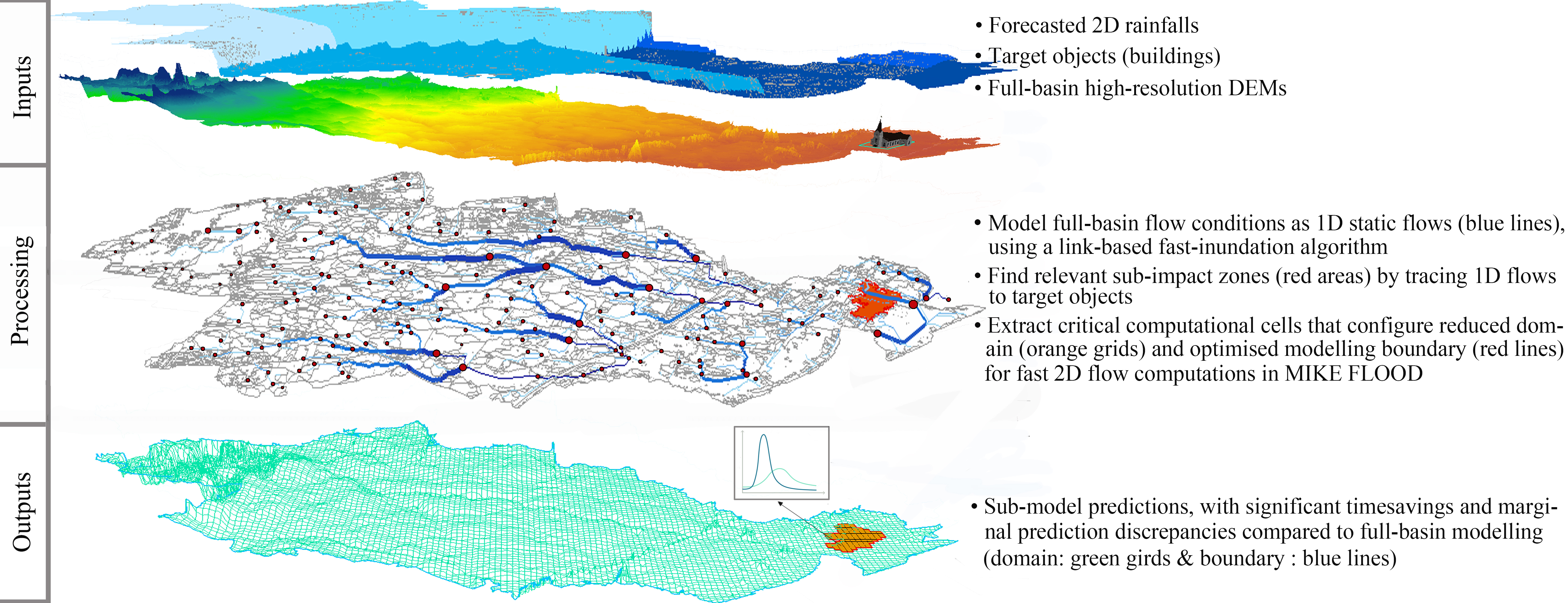
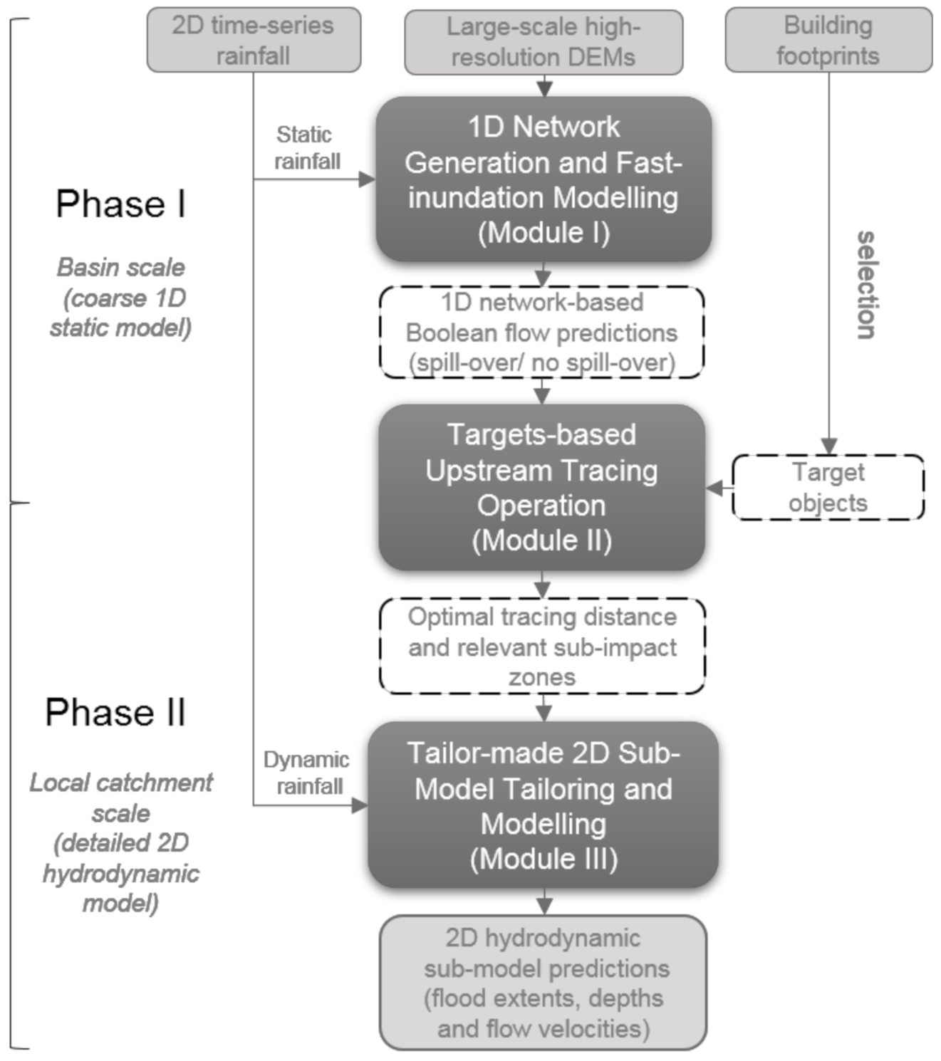
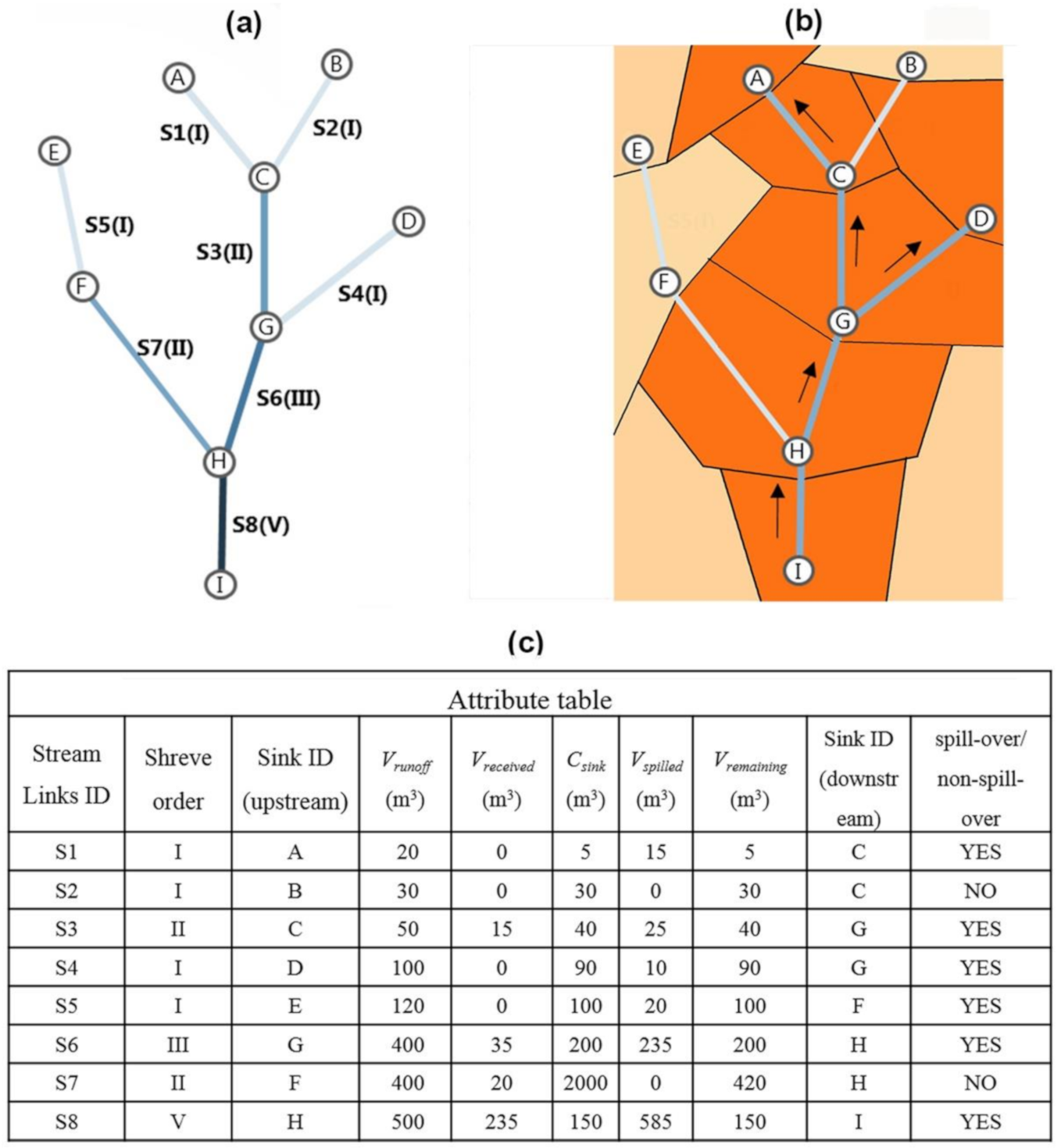
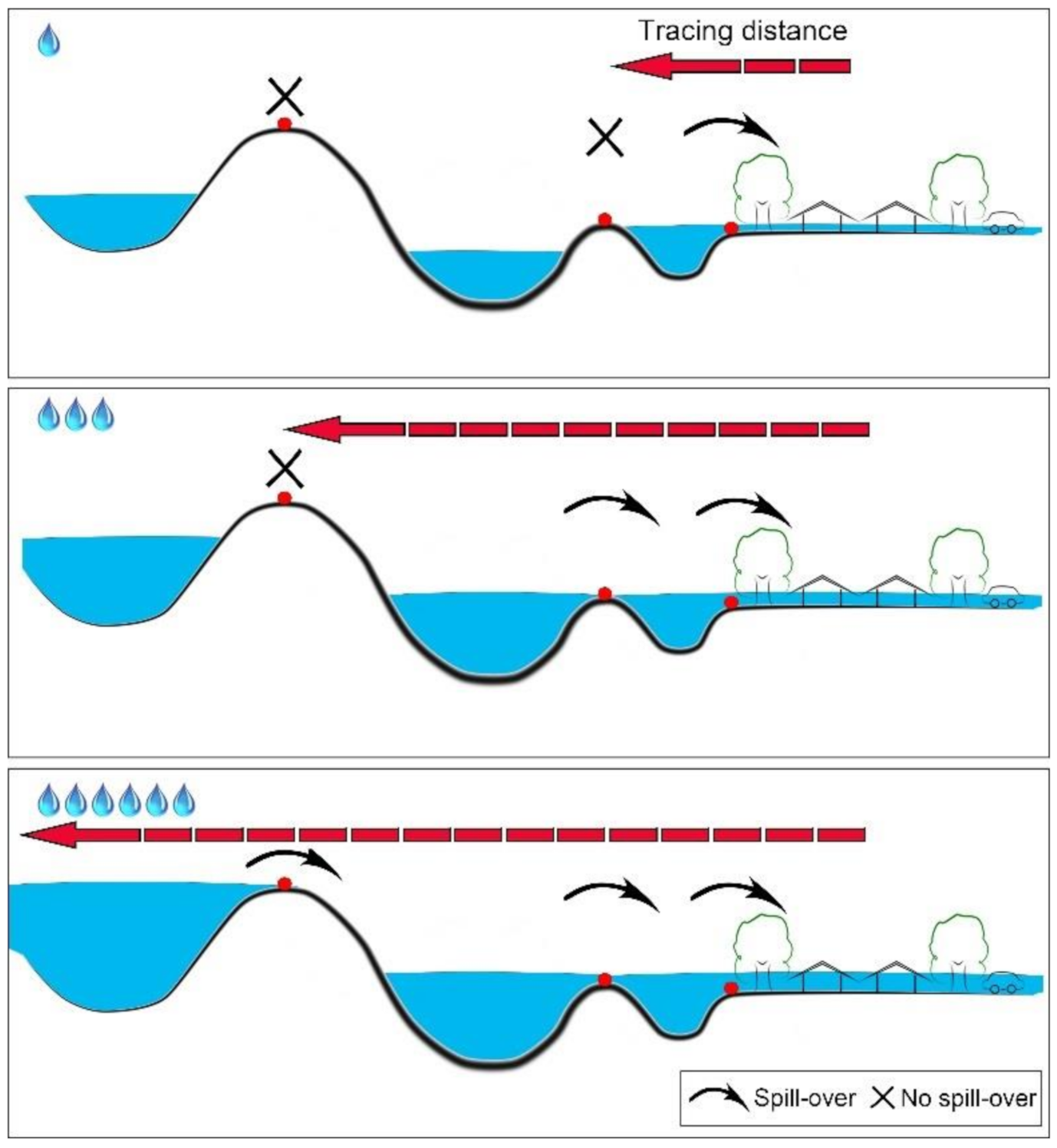
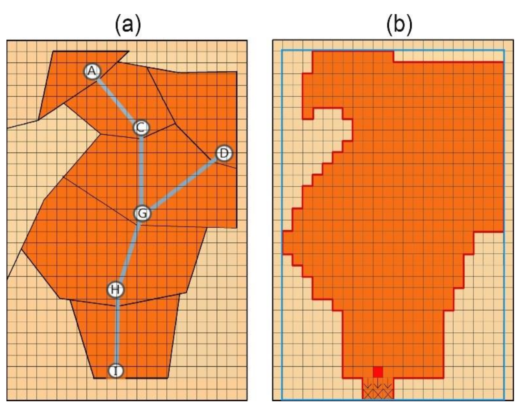
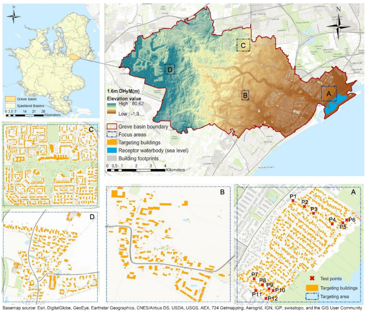
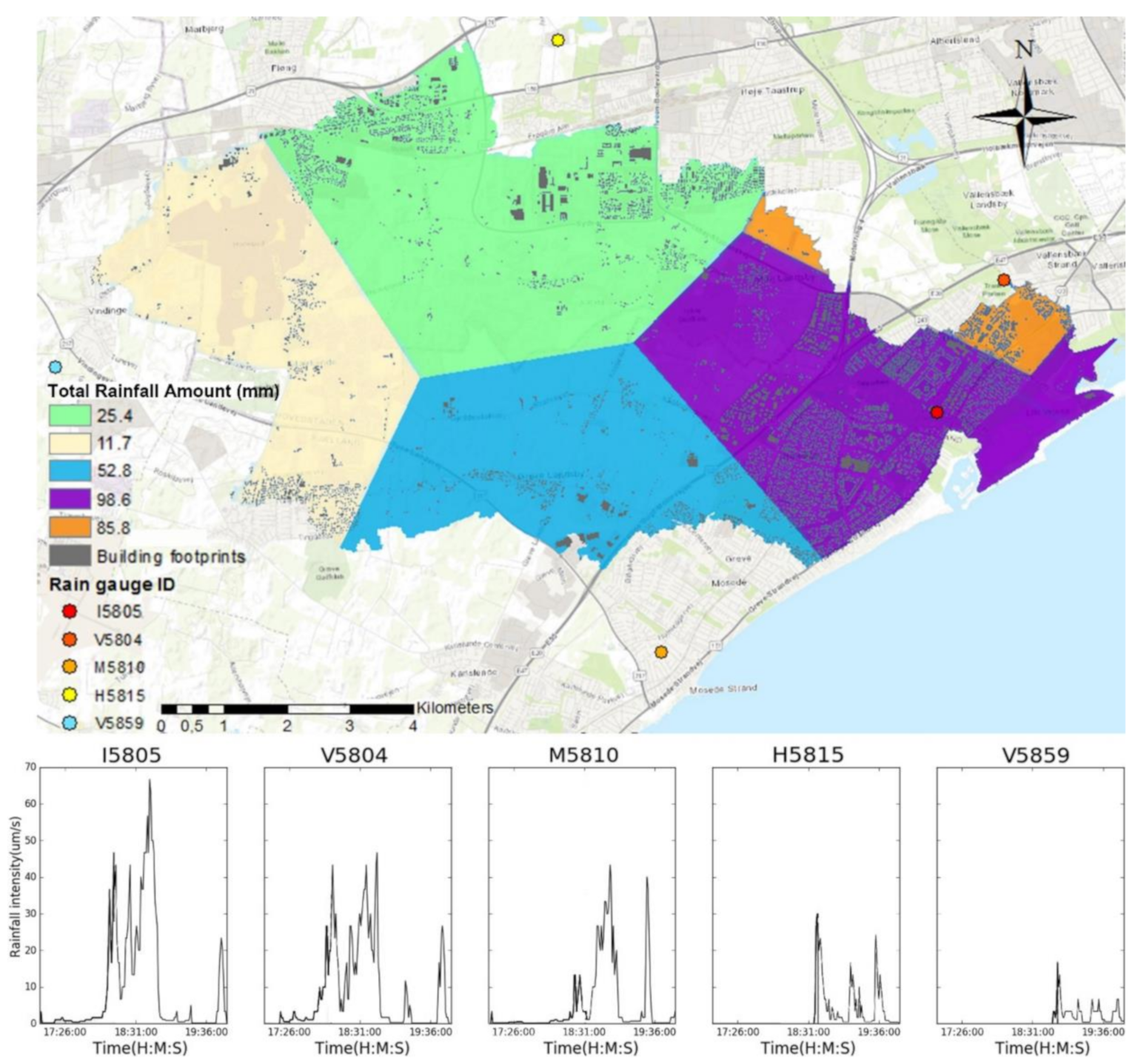
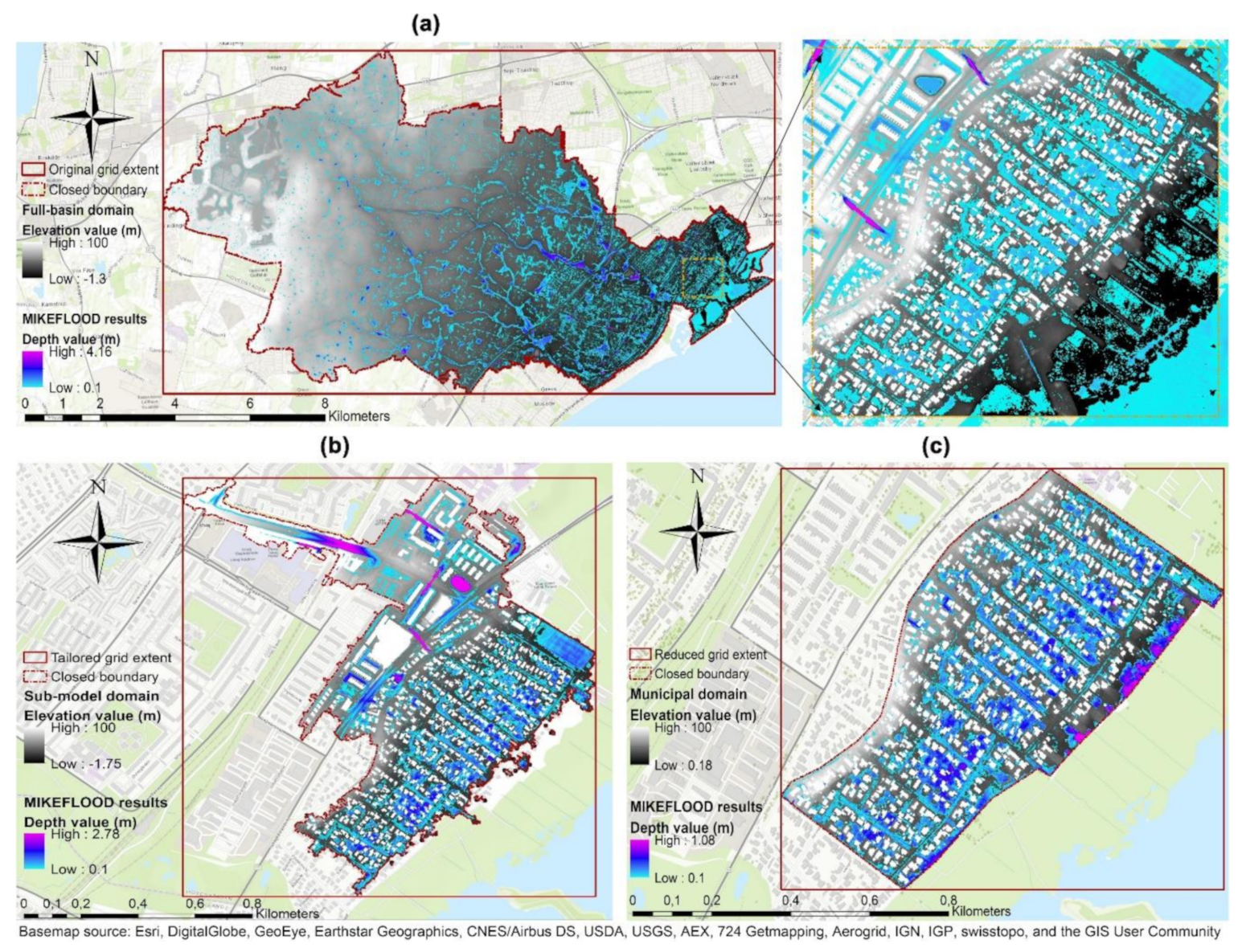
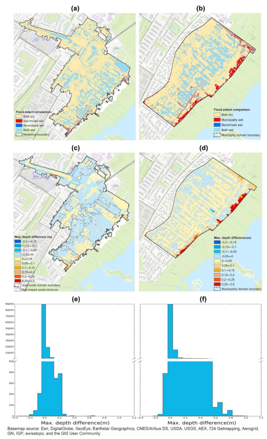
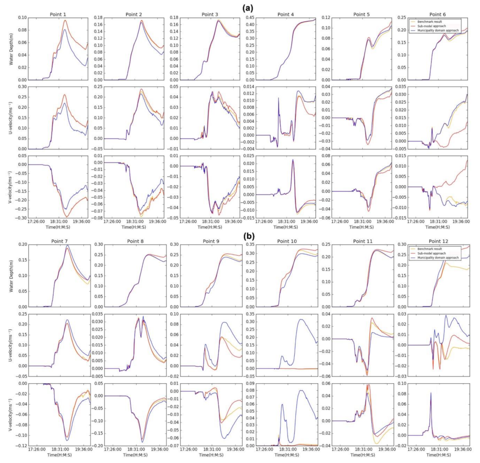
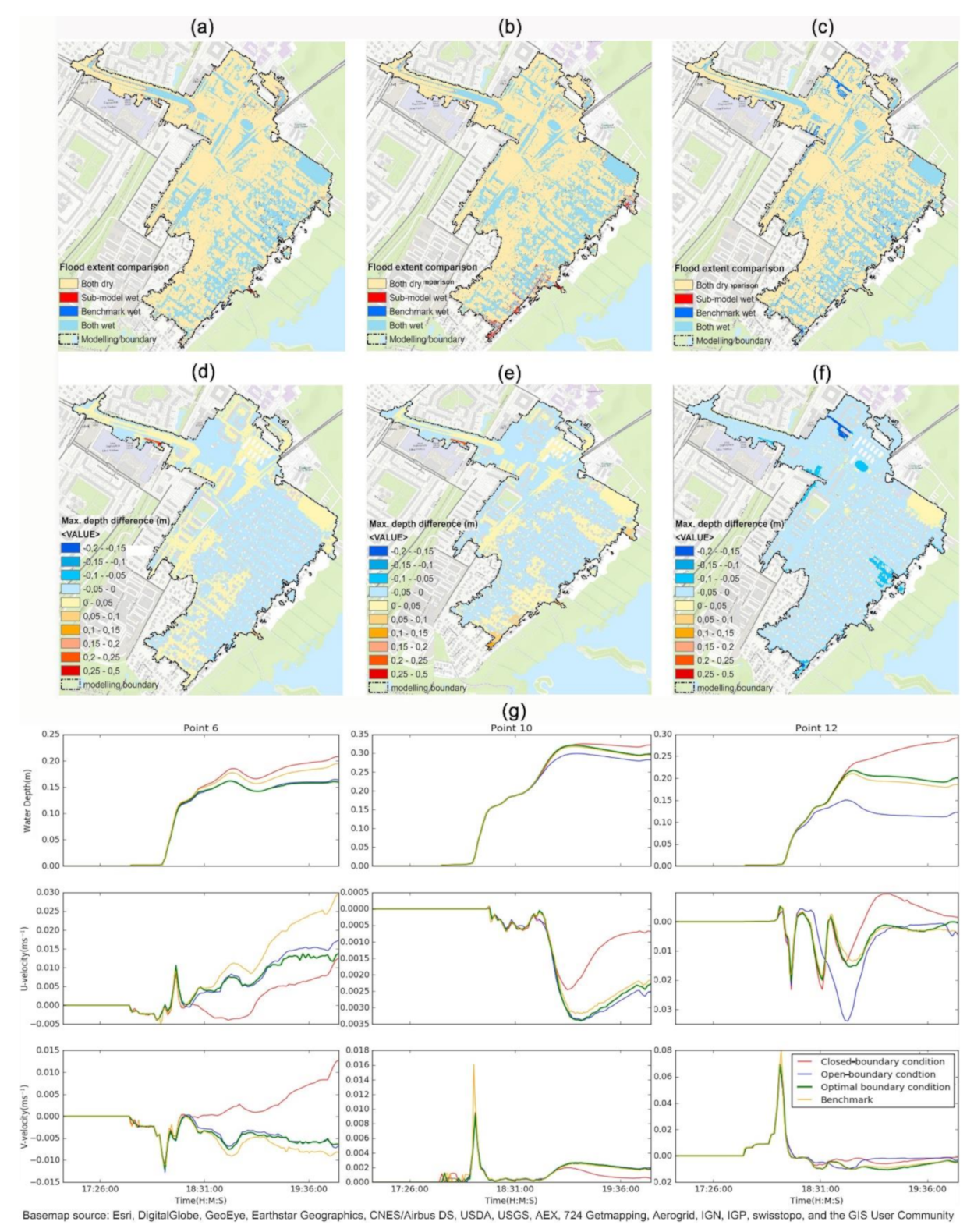
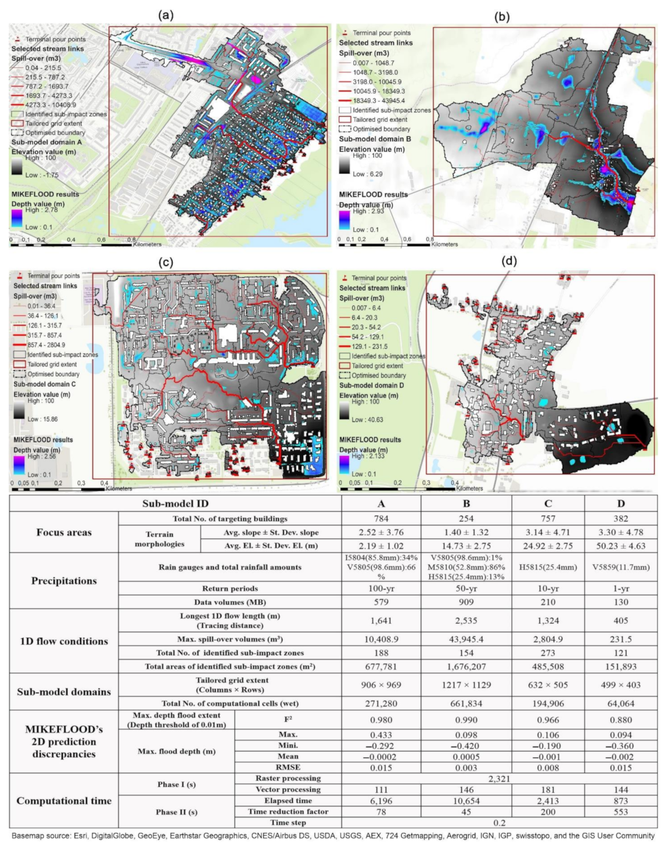
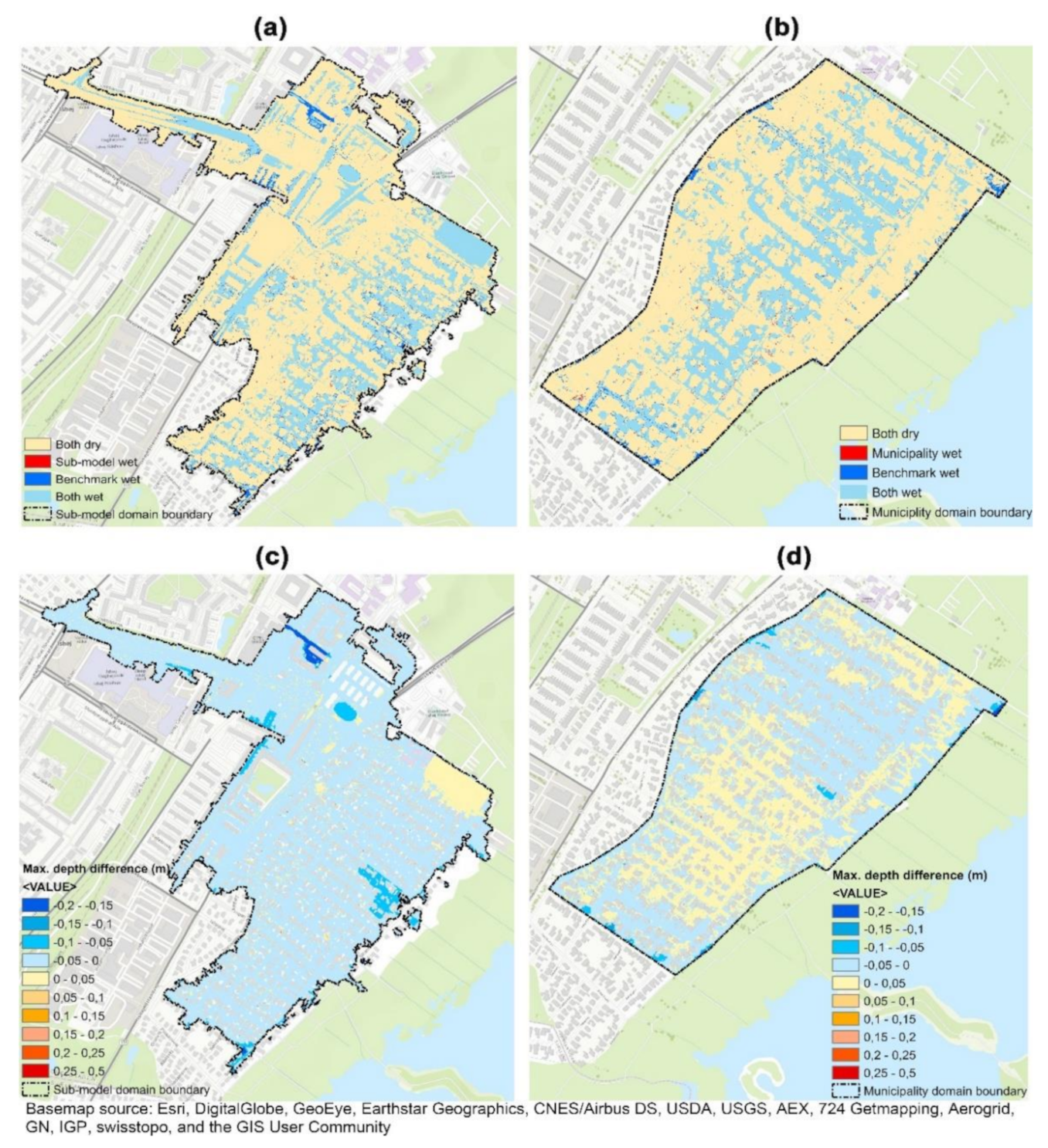
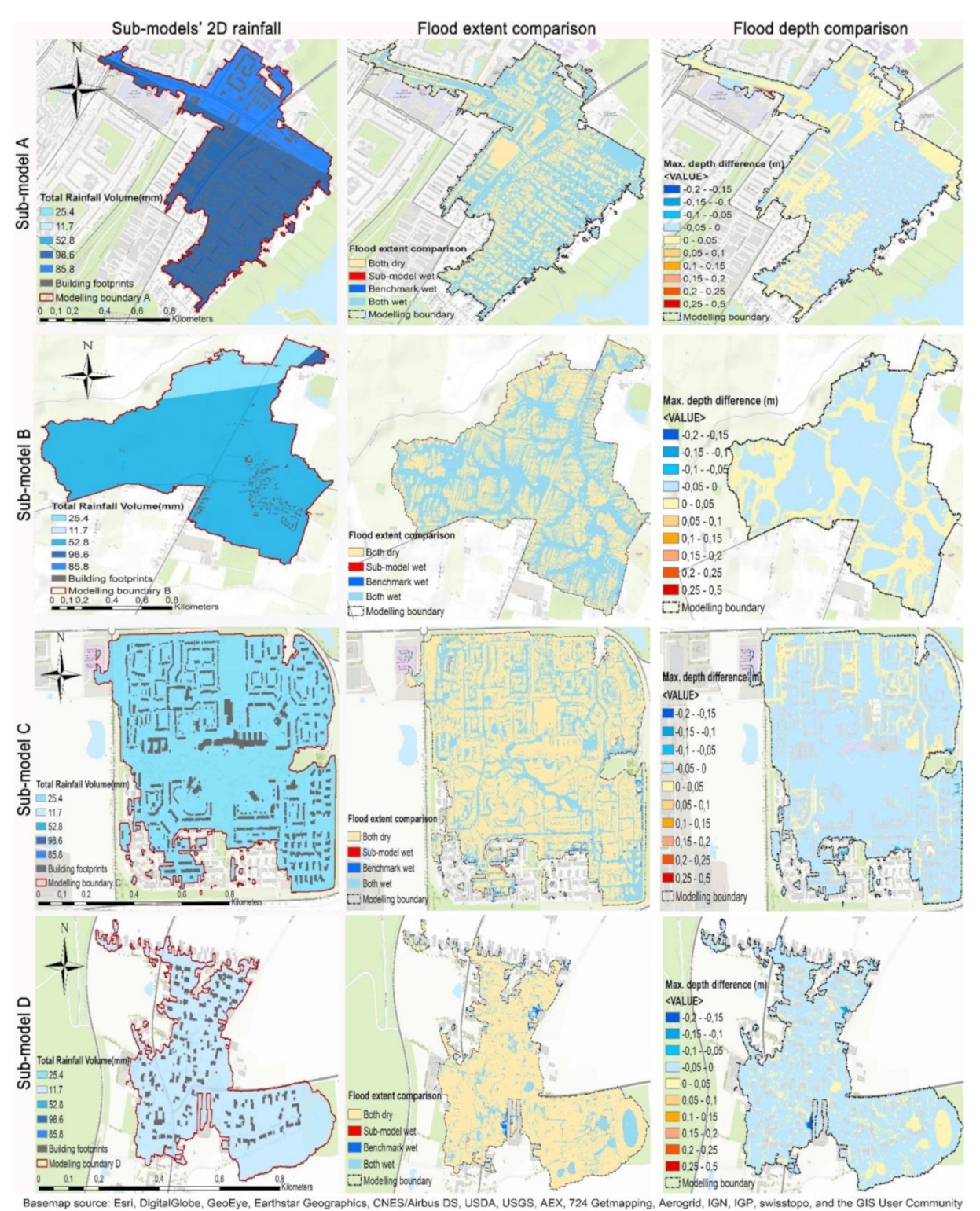
Table 1.
F2 values for the sub-model approach vs. the municipality domain approach.
| Depth Threshold (m) | 0.01 | 0.05 | 0.1 | 0.15 | 0.2 | 0.25 | 0.3 | 0.35 | 0.4 |
|---|---|---|---|---|---|---|---|---|---|
| Sub-Model Approach F2 | 0.97 | 0.95 | 0.94 | 0.93 | 0.92 | 0.92 | 0.91 | 0.91 | 0.91 |
| Municipality Domain Approach F2 | 0.91 | 0.86 | 0.81 | 0.77 | 0.73 | 0.69 | 0.60 | 0.50 | 0.32 |
Table 2.
Statistics of flood maximum depth difference for the sub-model approach vs. the municipality domain approach.
Table 2.
Statistics of flood maximum depth difference for the sub-model approach vs. the municipality domain approach.
| Overall Domain | Targeting Section | |||||||
|---|---|---|---|---|---|---|---|---|
| Minimum (m) | Maximum (m) | Mean (m) | RMSE (m) | Minimum (m) | Maximum (m) | Mean (m) | RMSE (m) | |
| Sub-model approach | −0.37 | 0.68 | 0.00 | 0.02 | −0.22 | 0.36 | 0.00 | 0.02 |
| Municipality domain approach | −0.23 | 1.02 | 0.02 | 0.08 | −0.23 | 0.43 | 0.01 | 0.02 |
Table 3.
Comparison of computational efficiency when using different domain approaches.
| Full-Basin Domain Approach | Sub-Model Approach | Municipality Domain Approach | ||
|---|---|---|---|---|
| Input DEM’s grid extent (Columns × Rows) | 10,202 × 5263 | 10,202 × 5263 | 10,202 × 5263 | |
| Tailored grid extent (Columns × Rows) | × | 903 × 967 | 701 × 612 | |
| Total No. of computational cells (wet) | 27,124,785 | 263,278 | 148,258 | |
| Pre-processing time (s) (Phase I) | Raster processing | × | 2321 | × |
| Vector processing | × | 111 | × | |
| MIKE FLOOD simulation time (Phase II) | Elapsed time (s) | 482,412 | 6090 | 2903 |
| CPU time (s) | 1,141,666 | 24,330 | 11,585 | |
| Time step (s) | 0.2 | 0.2 | 0.2 | |
Publisher’s Note: MDPI stays neutral with regard to jurisdictional claims in published maps and institutional affiliations. |
© 2021 by the authors. Licensee MDPI, Basel, Switzerland. This article is an open access article distributed under the terms and conditions of the Creative Commons Attribution (CC BY) license (http://creativecommons.org/licenses/by/4.0/).
Share and Cite
MDPI and ACS Style
Zhao, G.; Balstrøm, T.; Mark, O.; Jensen, M.B. Multi-Scale Target-Specified Sub-Model Approach for Fast Large-Scale High-Resolution 2D Urban Flood Modelling. Water 2021, 13, 259. https://doi.org/10.3390/w13030259
AMA Style
Zhao G, Balstrøm T, Mark O, Jensen MB. Multi-Scale Target-Specified Sub-Model Approach for Fast Large-Scale High-Resolution 2D Urban Flood Modelling. Water. 2021; 13(3):259. https://doi.org/10.3390/w13030259
Chicago/Turabian StyleZhao, Guohan, Thomas Balstrøm, Ole Mark, and Marina B. Jensen. 2021. "Multi-Scale Target-Specified Sub-Model Approach for Fast Large-Scale High-Resolution 2D Urban Flood Modelling" Water 13, no. 3: 259. https://doi.org/10.3390/w13030259
Note that from the first issue of 2016, this journal uses article numbers instead of page numbers. See further details here.