An Integrated Modeling System for the Evaluation of Water Resources in Coastal Agricultural Watersheds: Application in Almyros Basin, Thessaly, Greece

Abstract

This study presents an integrated modeling system for the evaluation of the quantity and quality of water resources of coastal agricultural watersheds. The modeling system consists of coupled and interrelated models, including (i) a surface hydrology model (UTHBAL), (ii) a groundwater hydrology model (MODFLOW), (iii) a crop growth/nitrate leaching model (REPIC, an R-ArcGIS-based EPIC model), (iv) a groundwater contaminant transport model (MT3DMS), and (v) a groundwater seawater intrusion model (SEAWAT). The efficacy of the modeling system to simulate the quantity and quality of water resources has been applied to the Almyros basin in Thessaly, Greece. It is a coastal agricultural basin with irrigated and intensified agriculture facing serious groundwater problems, such as groundwater depletion, nitrate pollution, and seawater intrusion. Irrigation demands were estimated for the main crops cultivated in the area, based on precipitation and temperature from regional weather stations. The models have been calibrated and validated against time-series of observed crop yields, groundwater table observations, and observed concentrations of nitrates and chlorides. The results indicate that the modeling system simulates the water resources quantity and quality with increased accuracy. The proposed modeling system could be used as a tool for the simulation of water resources management and climate change scenarios.

1. Introduction

Around the semi-arid Mediterranean basin, complex cases of water resources degradation, also characterized by poor quantity and quality status, are currently met in coastal agricultural basins. The complexity of the problems of such water systems arises mainly from: (i) the limited use of surface water, (ii) the excessive groundwater abstractions for irrigation, and (iii) the over-fertilization practices for crop yield magnification [1]. These actions cause the lowering of the water table of aquifers, increase nitrate groundwater pollution, and invoke seawater intrusion to groundwater systems [2]. Groundwater pollution has an important role among water resources management strategies due to the majority of the semi-arid regions it is encountered. Some known examples of coastal water systems where intensive agricultural practices, for irrigation and fertilization purposes, have caused serious degradation of the groundwater resources and documented in the international literature, including Italy (Nurra region of Sardinia [3] and central-southern Italy [4]), south-eastern France (Lower Var Valley) [5], Spain (e.g., Mancha Oriental System in Jucar River Basin, Oropesa Plain, Vinaroz Plain) [6,7], Portugal (Tagus catchment) [8], Egypt (e.g., Bagoush plain, North Sinai area, East Nile Delta aquifer), Tunisia (Jerba Island), Algeria (Nador plain), Morocco (Bou-Areg aquifer) [9], Lebanon (Akkar and Damour aquifers), Syria (e.g., Latakia and Tartous groundwaters), Palestine (Gaza aquifer), Jordan (northern Jordan, Yarmouk Basin) [10], Cyprus (Magosa aquifer) [11], Turkey (e.g., Silifke-Goksu Deltai, Serik, and Tarsus Plains) [12], and in the Greek coastal areas.

According to the Greek Ministry of the Environment, many coastal aquifer systems experience groundwater depletion, nitrate pollution, and seawater intrusion in Greece [13,14,15]. Examples of water-stressed and polluted groundwater systems are located in Macedonia (Axios River basin, Galikos River basin), in Chalkidiki peninsula (Moudania watershed and Havrias River basin), in central Greece (Sperheios River basin, Voiotikos Kifisos River basin (the Kopaida Plain)), in Peloponnese (Plain of Argos and Pinios River basin), in Greek Islands (Crete), and in Thessaly (Pinios River basin and Almyros basin) [13,14,15].

In nitrate contaminated waters, the “threshold of concern” is 25 NO₃ mg/L, and mostly refers to the suitability of the drinking water. The upper safe concentration is set at 50 NO₃ mg/L while higher nitrates concentrations endanger human health, surrounding ecosystems, and local biodiversity [15,16]. Thresholds of chloride concentrations have been defined as well, for the groundwater systems of more than 10 Member States of the EU. According to the Directive 2006/118/EC, the maximum allowable concentrations of chlorides range between 24 Cl mg/L and 12,300 Cl mg/L, in reliance on the diversity of characteristics of groundwater systems. The maximum allowable concentration of chlorides for urban water supply is set at 250 Cl mg/L, while in higher concentrations its consumption is traceable in taste and is also linked to health problems [17].

Hence, research must be done in the direction of the development of efficient software and tools that take into account the impacts of water abstractions, the water balance deficit, the nitrate leaching, the nitrate pollution, and the seawater intrusion [18,19,20,21]. Until recently, most of the hydrological processes and human interactions either for surface water resources [22] or groundwater [23], or under climate change [6] or land uses [24], or landscape and population changes [25] are often studied separately. The connection and communication of surface water and groundwater [26], the unsustainable water use [1,27], the irrational fertilization of crops [2], the groundwater contamination, the head dropdown of coastal aquifers [28], their salinization [29,30], and the reduced yields of crops [31] are rarely modeled in an integrated modeling system. Consequently, the simulation of the spatiotemporal responses of the water resources systems, in view of an integrated modeling system, can advance the reliability of fully understanding and modeling the complex interactions of water systems. A holistic approach of the natural and socio-economic drivers that may cause quantitative and qualitative problems of water resources, can further promote their effective management and the configuration of improvement strategies [32]. In this direction, very recent examples of integrated modeling of water resources quantity and quality are documented in the literature; such as the Community Water Model for the quantitative simulation of water resources [33], the remote sensing and GIS-based conceptual model of land use change impacts on groundwater quantity and salinity [34], the coupled models of groundwater flow and particle tracking of contaminants in karstic groundwater bodies [35], the Bow River Integrated Model (BRIM) for the simulation and management of water resources at basin scale [36], the FREEWAT, a QGIS based simulation and management system of coupled models of surface and groundwater quality and quantity, and agricultural water uses [37], the national-scale conceptual model for nitrate transport and dilution in aquifers [38], the modeling system of nonconservative contaminants in variable-density flow [4], and the Integrated Hydrological Modeling System (IHMS) for the simulation and management of surface and groundwater resources and saltwater intrusion [39]. Under the concept of the development of an integrated modeling system, adequate resolution in space and in time is of critical importance, in order to achieve faithful results, reduced inherent uncertainty, effective modeling of heterogeneity and of parameter variability, and reduced calibration/validation times [32].

The major research question that the paper tries to answer is how to efficiently simulate the integrated water balance and water quality of groundwater resources of coastal agricultural watersheds at a basin/watershed scale. This study aims to address this question with the development of an integrated modeling system, which includes coupled and interrelated models of surface and groundwater hydrology, a crop growth/nitrate leaching model, and groundwater models for the simulation of groundwater, nitrate contamination, and seawater intrusion, set up for use in agricultural coastal watersheds. The modeling system has been applied in the Almyros basin, a significant coastal region with intense agricultural activity, located in Thessaly, central Greece. The modeling system has been calibrated and validated against observations and applied to reproduce the water resources, mainly groundwater, quantity, and quality for the period of October 1991 to September 2018.

The simulation results indicated that the proposed modeling system simulates the water resources quantity and quality, with increased accuracy, and could be used as a tool for the simulation of alternative water resources management scenarios and water resources management. Especially, for the Almyros basin, the causes of the deficit water balance are determined to be (i) the increased water well pumping during the crop growth summer periods, (ii) the absent use of surface water for irrigation, and (iii) the possible unsuitability of crop types to the regional semi-arid climate. This, in turn, led to the inland salinization of the coastline areas. Furthermore, the nitrates assimilation into the aquifer originates from the nitrates leached during crop irrigation and rainfall as a result of the excess fertilization applications. The integrated modeling system and its application in the Almyros Basin is described in the following sections.

2. Models and Methods

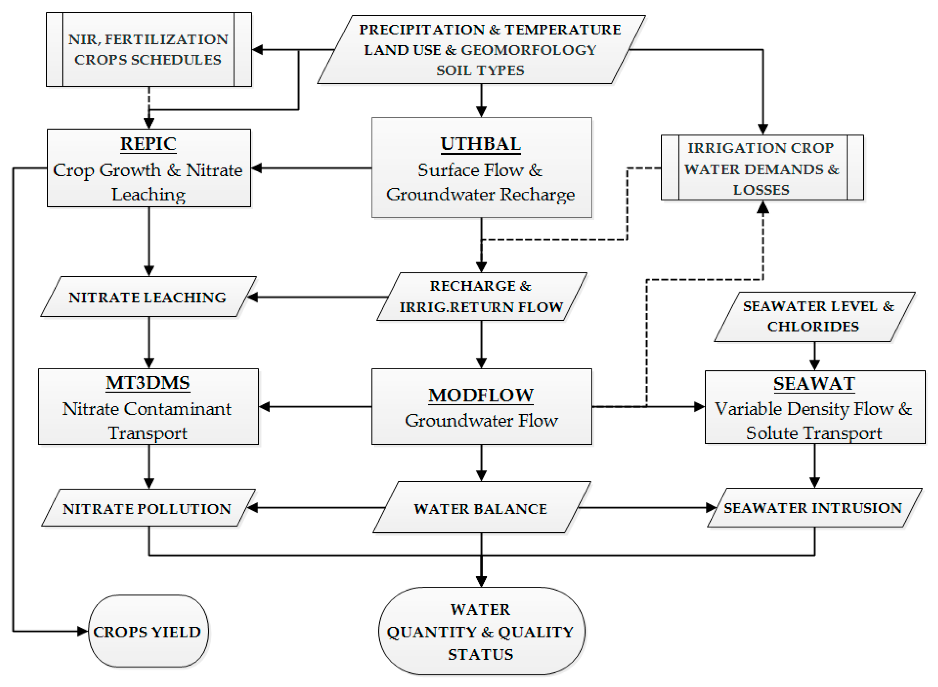
2.1. Modeling System

The scope of this study is to present the development of a modeling system for the evaluation of the surface water balance on a sub-basin scale, the crop water demands, the nitrates leached from the unsaturated zone, the groundwater quantity, and nitrate pollution and salinization in an aquifer system, on a grid-scale. The developed integrated modeling system consists of coupled simulation models of the natural processes of the hydrologic cycle, and the contamination events and their impacts. The components of the system are the models of surface hydrology (UTHBAL) [1], groundwater hydrology (MODFLOW) [40], crop growth/nitrate leaching (REPIC), which is an innovative R-ArcGIS user interface with the EPIC model [41], contaminant transport/ nitrate pollution (MT3DMS) [42], and seawater intrusion/aquifer salinization (SEAWAT) [43].

The mean monthly areal precipitation, temperature, and evapotranspiration are used as inputs in the surface hydrology model (UTHBAL). The model estimates the monthly surface runoff and the natural groundwater recharge per sub-basin. The weighted average irrigation return flow per sub-basin and main crop category are, then, added to the recharge rate, as calculated in the previous step. The sum of natural recharge and irrigation return flow is the input flows of the groundwater model (MODFLOW). To address the crop water demands, abstraction water well flows are determined as the outflows of the aquifer. The input of the sea level head completes the water balance of the model. In the context of this research, the distributed crop growth/nitrate leaching simulation model REPIC was developed, along with tools for efficient and easy interaction with the models of UTHBAL and MT3DMS. REPIC model is a spatially distributed model, similar to GEPIC [44], as it simulates every grid cell area as a field. It is based on the R-programming language [45] with the R-ArcGIS Bridge [46] in ArcGIS 10+/Pro, and the public domain Environmental Policy Integrated Climate (EPIC) model. EPIC model is used as is, compiled in Fortran and as provided individually by [47]. It is an agro-hydrological model that simulates and estimates, among other parameters, the nitrates leached into the groundwater. Subsequently, the nitrates leached are the input contaminant flows of the MT3DMS model. The modeling system is completed with the simulation of the seawater intrusion of the aquifer. The chloride concentration of the sea is the input chloride inflow of the SEAWAT model. Finally, the quantity and quality status of the coastal water resources can be defined. More details about the models are described in the next paragraphs. The flow chart of the integrated modeling system is illustrated in Figure 1.

2.1.1. Surface Hydrology Simulation Model Description

The UTHBAL model is a surface hydrology model that can simulate the surface runoff and groundwater recharge, developed by Loukas et al. in 2007 [1]. UTHBAL uses as inputs monthly time series of precipitation, mean temperature, and potential evapotranspiration. The water balance model separates the total precipitation into rainfall and snowfall and calculates the snowpack and snowmelt. The model divides the total watershed runoff into three components: the surface runoff, the interflow, and the baseflow using a soil moisture mechanism. The first priority of the model is to fulfill the actual evapotranspiration. The output of the model is watershed runoff, actual evapotranspiration, groundwater recharge, and soil moisture.

The model can be applied as a lumped, semidistributed, and fully-distributed model depending on the available data. The model contains six parameters that are estimated during the calibration process, based on surface runoff monthly observations. These are, the parameter of monthly melt rate factor, Cm, the coefficient of actual evapotranspiration, α, the coefficient of interflow β, the coefficient of baseflow, γ, the coefficient of groundwater recharge, K, and the Curve Number of the US Soil Conservation Service [48].

In this study, the surface hydrology model (UTHBAL) has been used for the estimation of the monthly surface runoff and the monthly groundwater recharge. The UTHBAL model has been applied as a semidistributed model simulating the surface hydrological processes of six sub-basins of the Almyros basin from October 1961 to September 2018. For the estimation of areal precipitation, the gradient method modified with the Thiessen polygon method were combined [49,50,51]. The steps followed in the procedure are:

• Multiplication of the precipitation time-series of each station with the respective Thiessen polygon ratio of a sub-basin. The Thiessen areal precipitation, P_th, is considered at the mean elevation of the sub-basin.
• The correction of the estimation of the mean areal precipitation is performed with the monthly precipitation gradient of the whole basin. The reduction to the mean elevation of the sub-basin, Y_b, from the elevation of each station, Y_st, is equal to their difference, dh:

  $$dh={\displaystyle \sum }\left(Y_b-Y_{st}\right) \left[\mathrm{m}\right]$$

  (1)
• The corrected areal precipitation, P_b, attributed to the mean elevation of each sub-basin is given by the equation:

  $$P_b=P_{th}+\beta ·\left({{\rm Y}}_b-Y_{st}\right) \left[\mathrm{mm}\right]$$

  (2)

The estimation of the mean monthly temperature was estimated with the gradient method and the potential evapotranspiration was calculated with the Thorthwaite method [52]. The UTHBAL model has been successfully applied, calibrated, and validated in various Mediterranean regions, like Crete, Cyprus, Nestos/Mesta Basin, Thessaly [1], and in the neighboring areas of Pinios River Basin and Karla Basin [16,53].

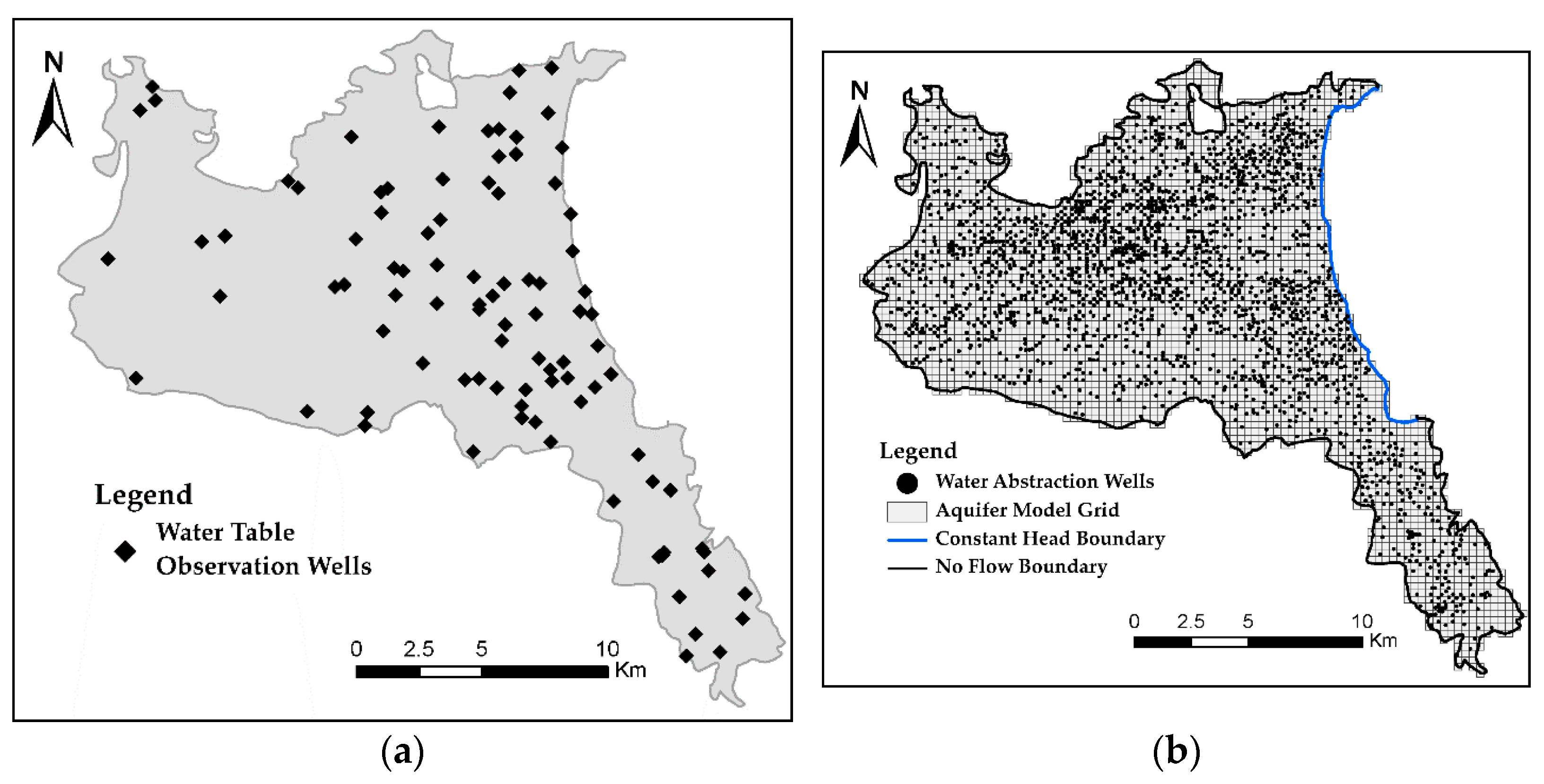
2.1.2. Groundwater Flow Model Description

MODFLOW is a software application that mathematically resolves the three-dimensional groundwater flow equation in a porous medium [40]. The partial differential equation that describes groundwater flow, Equation (3), results from the application of the equation of conservation of mass and Darcy’s law. McDonald and Harbaugh [54] have originally reported that MODFLOW simulates steady and transient water flow by using the finite difference method with a block-centered approach. The model was updated by Harbaugh and McDonald in 2000 and this version became the most used by scientists since.

$$\frac{\vartheta }{\vartheta x}\left(K_{xx}\frac{\vartheta h}{\vartheta x}\right)+\frac{\vartheta }{\vartheta y}\left(K_{yy}\frac{\vartheta h}{\vartheta y}\right)+\frac{\vartheta }{\vartheta z}\left(K_{zz}\frac{\vartheta h}{\vartheta z}\right)+W=S_s\frac{\vartheta h}{\vartheta t}$$

(3)

where, (i) xx, yy, zz are the axes of the Cartesian system, in which the components of the hydraulic conductivity of the aquifer, are attributed parallel to their positive directions, (ii) h is the hydraulic head, (iii) W is the water flux into or out of the system per time-step of each stress period, (iv) S_s is the specific storage of the hydrogeological formation, and (v) t is the time-step of the stress period simulated.

In a variably structured model grid, the aquifer is divided in layer(s), which can be confined, unconfined, or a mixture of confined and unconfined representing a homogeneous-heterogeneous isotropic, or anisotropic aquifer system. Furthermore, the model layer(s) can be inclined, or not, and have different cell sizes and layer thickness. MODFLOW is capable of simulating water flow originating from sources out of the aquifer model, and from physical causes of groundwater movement; such are the water abstraction flow rates of wells, constant hydraulic head bodies, and groundwater recharge. These are represented mathematically with boundary conditions and incorporate the solution of Equation (1). The main water flow boundary conditions are the hydraulic head along an aquifer’s margins (Dirichlet Condition), the hydraulic head gradient across an aquifer’s boundaries (Neumann Condition), and the combination of the two (Cauchy Condition). The hydraulic head variations are, then, calculated for each time-step of the simulated stress period [40].

The groundwater hydrology model MODFLOW has been used for the simulation of groundwater flow and the estimation of the water balance of the Almyros aquifer. MODFLOW has been successfully applied in aquifer systems in Greece such as in the Lake Karla aquifer [16,53,55], in Eidomeni-Evzones region in Axios basin [56], in Moudania aquifer [57], on Thira aquifer in Santorini island [58,59], in Glafkos aquifer in Patras Gulf [60], in Cyclades [61], and in Messara aquifer system in Crete [62].

2.1.3. Nitrate Leaching Simulation Model Description

The REPIC model is a new model developed in the context of this research and firstly introduced in this study. The REPIC model is a spatially distributed nitrate leaching and crop growth model, based on the Environmental Policy Integrated Climate (EPIC) model and the R-programming language with the R-ArcGIS Bridge in ArcGIS 10+/Pro. REPIC also integrates the groundwater recharge from the surface hydrology model, UTHBAL, in the estimation of the nitrate leaching in mg/L.

The EPIC model was initially introduced for the simulation of the impacts of soil erosion on soil productivity in small watersheds, for up to 100 ha, by Williams et al. in 1984 [63]. The model was introduced to be the Environmental Policy Integrated Climate model, when it was enriched with functions for many environmental problems. Some of the modules that have been incorporated in the EPIC model, by William et al. in 1995 [41], are the crop growth and cultivation management practices, and the nitrogen and pesticide transport functions [64]. The operation results of crop growth and nitrate leaching, which are closely related to the quantity and quality of water resources, are the ones used in the REPIC model. Particularly, in the EPIC model, the estimation of the nitrate leaching quantity from the soil layers of the unsaturated zone is calculated by the Equation (4) [65]:

$$C_{N{O}_3}=\frac{V_{N{O}_3}}{QT}$$

(4)

where, C_NO3 is the average daily concentration in a quantity of water height, QT, and V_NO3 is the amount of NO₃-N lost from the unsaturated zone towards groundwater.

Similarly, the crop yield of the simulated crop types is calculated by the Equation (5) [65]:

$$YL{D}_j=H{I}_j·B_{AG}$$

(5)

where, YLD_j is the crop yield of crop j, HI_j is the harvest index of the crop j, and B_AG is the above-ground biomass extracted in harvest.

Considering the aforementioned, the spatially distributed modeling of the EPIC model is performed with programming languages that form a Graphical User Interface with the EPIC model. Such programming languages are the Visual Basic and Python, and the R. Previous examples of spatially distributed modeling of the EPIC model are the GEPIC model, a Visual Basic-based EPIC model, and the PEPIC model, a Python-based EPIC model [66].

The REPIC model is an R-ArcGIS based model. The REPIC model simplifies the procedure of the creation of the input data files, because it uses as input data a point shapefile with all the required characteristics of the grid-cell areas. The points are the coordinates of the centroids of the grid cells, their elevation, area, crop type, maximum NIR, nitrate loading, weather file code, and soil file code of the EPIC model. The simulation is performed considering different crop types in every grid cell, as opposed to GEPIC that simulates all grid cells as only one crop type per simulation run. REPIC also solves the restrictions of the GEPIC model for regional simulations, which are: (i) the stepping into the GEPIC’s VBA code to change the geographical extent of the simulated area and also to increase the grid’s resolution, and (ii) the dependence from the UTIL executable that inputs the data to the EPIC files. Moreover, relevant tools were designated for the manipulation of the input data. These are (i) the EPIC Parameter tool, which changes the values of hydrological parameters, (ii) the NIR tool, which assigns the NIR to each crop type, (iii) the NLD tool, which assigns the nitrate loading per crop type, (iv) the Nitrate Leaching tool, that reads the results, integrates the groundwater recharge from the UTHBAL model, and calculates the nitrate leaching in mg/L, (v) the Crop Yield tool, which calculates the spatial distribution of crop yields, and the (vi) DataForMT3DMS tool, which produces the estimated nitrate leaching in mg/L of all grid cells, on a monthly step, in .txt format ready for direct input into the MT3DMS model. Especially, the flexibility of the R programming language and the type of input file, which is a shapefile, creates the opportunity to downscale to finer resolutions if available data exist, and even to field-scale simulations of hydrological basins.

Spatially distributed modeling of the EPIC model, especially of the GEPIC model, has been successfully applied, calibrated, and validated in global gridded scale for wheat yield [44], maize [67], rice [68], crop water productivity, and drought risk assessment [44] in Sub-Saharan Africa [69], in country scale, in China [70], and in regional scale in Jordan River Basin [71], and in Karla Basin, Greece [53]. The PEPIC model has been also successfully applied in global scale for nitrogen losses [66].

The nitrate leaching/crop growth model REPIC has been used for the simulation of nitrate inflows in the groundwater system of Almyros, and the simulation and validation of crop yields in the Almyros basin. The nitrates leached into the groundwater, calculated with the REPIC model, are then added as input contaminant fluxes into the MT3DMS model.

2.1.4. Nitrate Transport and Dispersion Model Description

MT3DMS is a structural, three-dimensional, multispecies contaminant transport model, which can simulate advection, dispersion, and chemical responses of a groundwater system with dissolved compounds [42]. MT3DMS code is able to simulate pollutant and solute concentrations, while based on a solved problem of groundwater flow, most often provided by MODFLOW. MT3DMS is designed for interaction with any finite difference model, similar to MODFLOW. This linkage is feasible under the premise that concentration variations in space and time have negligible impact on the regional water flow pattern and that both codes share the same structure of the aquifer model [40,54].

MT3DMS solves the three-dimensional transport and dispersion of pollutants in the groundwater with the partial differential Equation (6) [42,72]:

$$\frac{\vartheta \left(\vartheta C^k\right)}{\vartheta t}=\frac{\vartheta }{\vartheta x_i}\left(\theta D_{ij}\frac{\vartheta C^k}{\vartheta x_j}\right)-\frac{\vartheta }{\vartheta x_i}\left(\theta v_i{C}^k\right)+q_s{C}_s^k+{\displaystyle \sum }{R}_n$$

(6)

where, (i) D_ij is the hydrodynamic dispersion coefficient tensor, (ii) C^k is the pollutant concentration in the aquifer system, (iii) C_s is the recharge, or outflow, concentration of the pollutant k, (iv) θ is the porosity of the hydrogeological formation, (v) x_{i, j} is the distance paved by the pollutant parallel to a Cartesian axis (here is xx axis), (vi) q_s is the volume of the pollutant’s flow rate attributed to each volumetric water flux, of an aquifer’s discrete grid-cell, (vii) v_i is the seepage or water velocity, (iix) ∑R_n is the component for the contaminant chemical production for n reactions, and (ix) t is the time-step of the stress period simulated.

The MT3DMS code simulates the flow of pollutants in the groundwater taking into consideration the advection, dispersion, and diffusion, and even chemical reactions. The differential term of Equation (6), ∂(θv_iC^k)/∂x_i, expresses the advection of the pollutant. The pollutant concentrations flow along with the transport medium, meaning at the same velocity as the groundwater flow. The hydrodynamic dispersion, D_ij, describes the characteristic of the pollutant to spread along the area of its location and cannot be estimated with the groundwater flow [42,73]. Hydrodynamic dispersion is equal to the sum of the mechanical dispersion and molecular diffusion. The mechanical dispersion stretches the pollutant concentrations along the vectors of the velocity deviations of groundwater velocity on the microscale. The molecular diffusion drives the pollutant molecules from areas with higher concentrations to areas with lower concentrations but is considered negligible, unless the groundwater velocity is very small. The parameter of longitudinal dispersivity (α_L) was calculated with the Neuman formula (1990) for water flow distance smaller than 3500 m [74]:

$${\alpha }_L=0.0175·L^{1.46}$$

(7)

where L is the water flow length, in this case, the grid size on the x-axis, and then it was calibrated to the hydraulic conductivity zones. The ratios of the horizontal transverse dispersivity to longitudinal dispersivity and the vertical transverse dispersivity to longitudinal dispersivity are kept in the default values of 1 and 0.1, respectively. The parameter of porosity is uniformly set to 0.3 according to literature for Neogene and Quaternary formations.

MT3DMS also simulates the sources of pollution as pollutant loadings in volume per unit volume of water flux. Moreover, sources of pollution are represented with concentration boundary conditions. Similarly to MODFLOW, these are the concentration along the aquifer’s margins (Dirichlet Condition), the concentration gradient across the aquifer’s boundaries (Neumann Condition), and the combination of the two (Cauchy Condition).

The groundwater contaminant transport model MT3DMS has been used for the simulation of nitrates transport and dispersion in the Almyros aquifer. MT3DMS has been successfully applied for the simulation of nitrate pollution in the Lake Karla aquifer system in Thessaly in Greece [16,53,55], in Vocha plain in Korinthos [75].

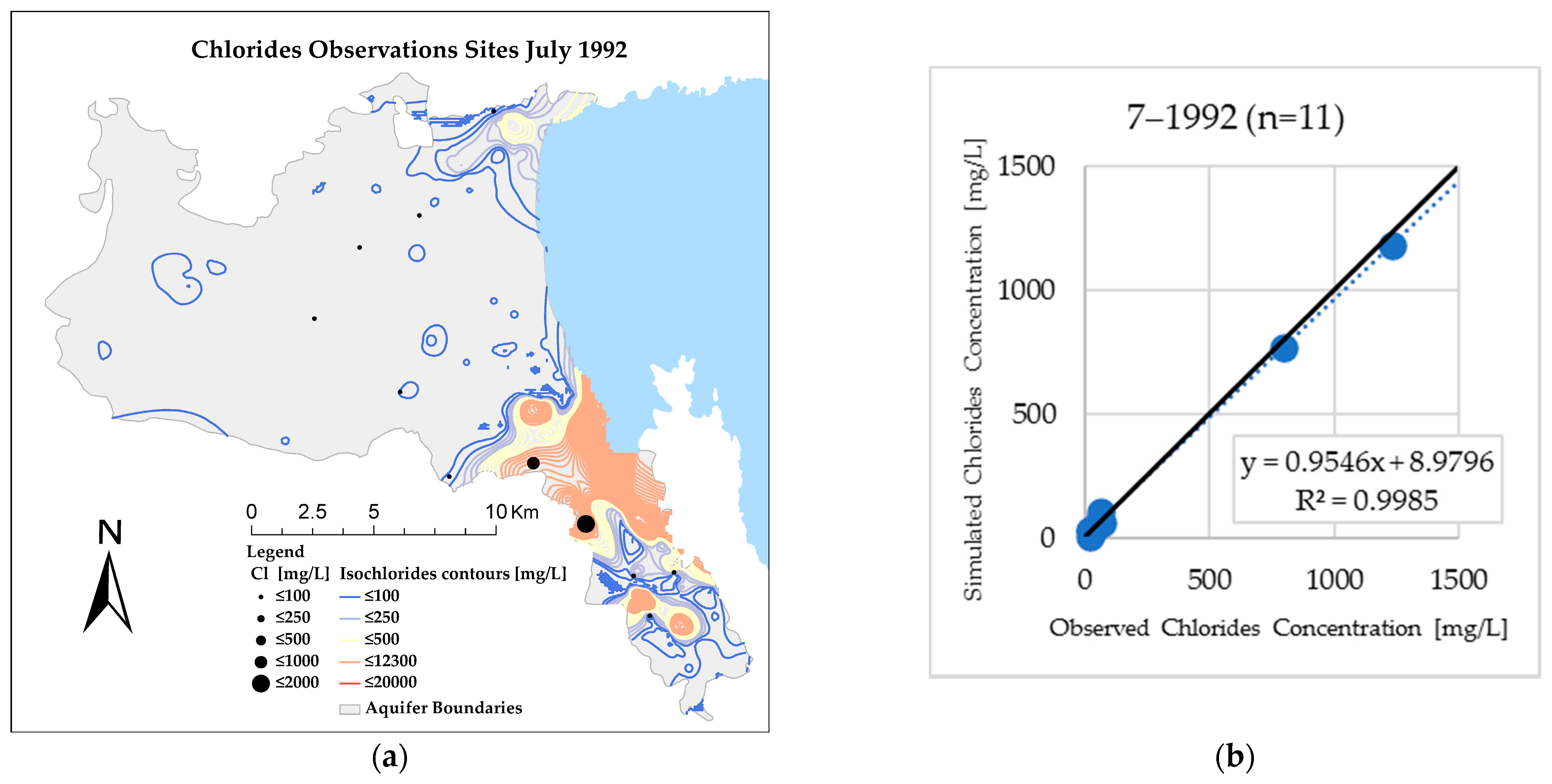
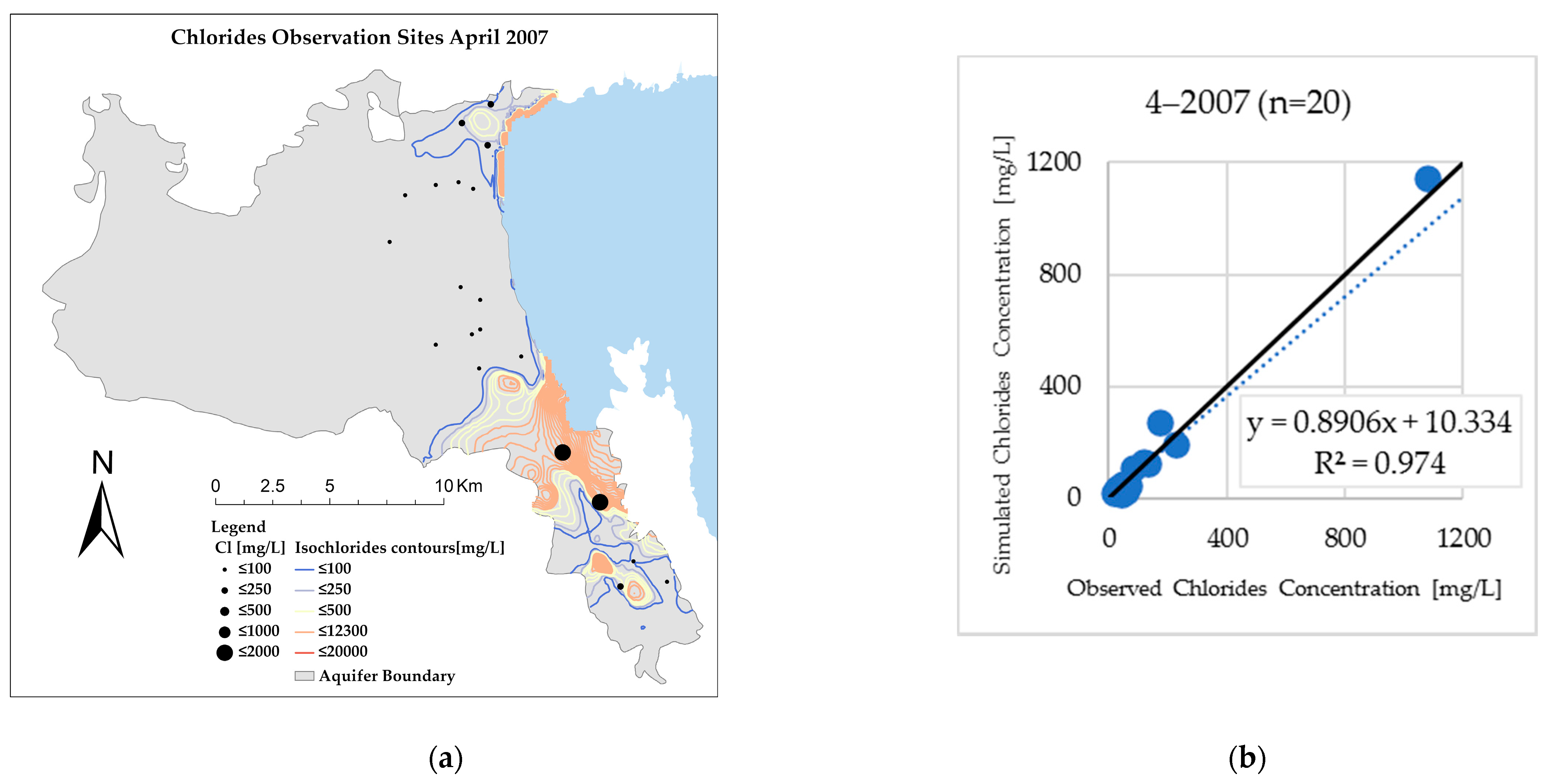
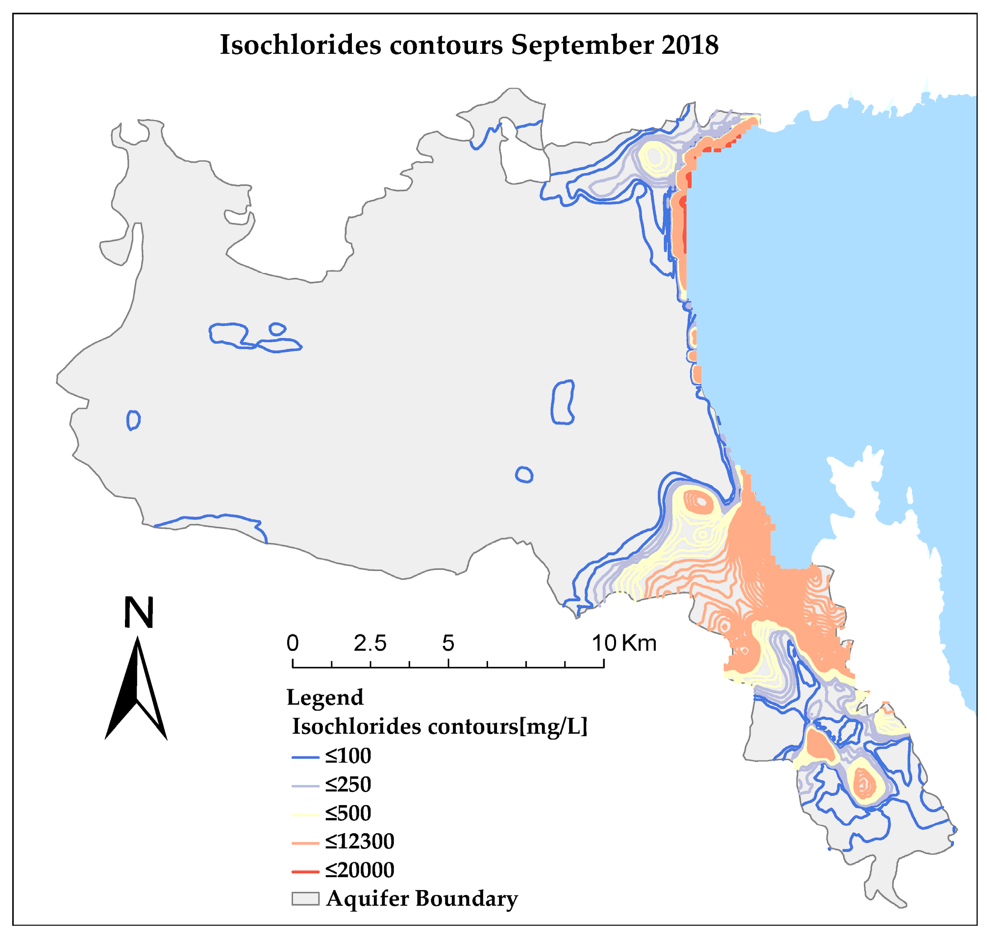
2.1.5. Chloride Solute Transport and Dispersion Model Description

SEAWAT is a finite difference, three-dimensional, modular transport model that simulates the variable density flow of water and solutes in porous aquifers. The concept of solving the variable density flow with the combination of MODFLOW and MT3DMS was first introduced by Guo and Bennett in 1998 [76]. The source code underwent several updates and its final version was developed by Guo and Langevin [43]. The code of SEAWAT merges the codes of MODFLOW and MT3DMS, while maintaining the consistency of the models’ structural characteristics and of the assumptions for groundwater flow and contaminant transport, regarding the advection and the hydrodynamic dispersion. The boundary conditions considered in a simulation with SEAWAT are exactly similar to the MT3DMS boundary conditions.

The presence of solutes in the groundwater in low concentrations does not have any effect on the fluid’s density, because the mass of the contaminant molecules is negligible. However, when the solute concentrations rise excessively, then their mass and density are increased accordingly and cause the water to move slower than the freshwater. This differentiation of the flow velocity of contaminated with solutes water, and of the freshwater, is studied as variable density flow [43]. Variable density flow is based on the concept of equivalent freshwater head. Equivalent freshwater head of a salinized hydraulic head, is the hydraulic head it would have, if there was not any solute contamination, if the fluid pressure is considered stable in the two states. The Equation (8) represents the dependance of salinized hydraulic head on the different fluid densities and freshwater head [43]:

$$h=\frac{{\rho }_f}{\rho }{h}_f+\frac{\rho -{\rho }_f}{\rho }Z$$

(8)

Initially, the groundwater flow with freshwater head, h_f, density ρ_f, and elevation, Z, is calculated by MODFLOW. The MT3DMS performs an update of the estimation of the fluid density,ρ, based on the solute concentrations. Then, the difference of the updated fluid density and the freshwater density is integrated in MODFLOW, which calculates the final water flow field due to variable fluid density.

Especially, seawater intrusion is a representative problem of variable density flow often simulated by SEAWAT. Due to the extravagant concentration of solutes in seawater, as related to fresh groundwater the fluid densities differ substantially. The fluid density of freshwater is 1000 kg/m³ and the fluid density of seawater is 1025 kg/m³.

SEAWAT has been successfully applied in coastal aquifer systems in Greece such as in Santorini island in Thira aquifer [58,59], in Cyclades [61], in Nea Moudania [57,77], in Glafkos aquifer in Gulf of Patras [60].

2.2. Statistical and Graphical Evaluation of the Models

Criteria of the goodness of fit of the simulated values against the observed measurements were incorporated, to evaluate the performance of the models REPIC, MODFLOW, MT3DMS, and SEAWAT in simulating the annual crop yields and the monthly groundwater flow, the monthly nitrate transport, and dispersion and the monthly chloride solute transport. The normal errors’ estimation of the Nash–Sutcliffe [78] Model Efficiency (Eff) (Equation (9)), the Coefficient of Determination (R²) [79] (Equation (10)), and the Index of Agreement (IA) [80] (Equation (11)) indicate the fit of the modelled to the observed values of variables.

$$Eff=1-\frac{{{\displaystyle \sum }}_{i=1}^n{\left(y_i-f_i\right)}^2}{{{\displaystyle \sum }}_{i=1}^n{\left(y_i-\overline{y}\right)}^2}$$

(9)

$$R^2=1-\frac{S{S}_{res}}{S{S}_{tot}}$$

(10)

$$IA=1-\frac{{{\displaystyle \sum }}_{i=1}^n{\left(y_i-f_i\right)}^2}{{{\displaystyle \sum }}_{i=1}^n{(\left|f_i-\overline{y}\right|+\left|y_i-\overline{y}\right|)}^2}$$

(11)

where (Y, F) represent the simulated and the observed values, SSres the sum of squares of residuals, and SStot the total sum of squares of the data.

The perfect agreement between the simulated and observed variables, all statistical criteria/measures (i.e., Eff, R², IA) take the value of 1. Values of the statistical criteria bellow 0,5 indicate a problematic/bad model and, as the values of the statistical criteria get values closer to 1, the model accurately simulates the observed variables.

Apart from the statistical evaluation of the modelled variables, the modelled and observed values of variables were drawn on maps and visually compared. Moreover, scatterplots were used to compare the modelled and observed values of the variables. The slope and intercept of the regression lines were statistically tested against the slope and intercept of the line of the perfect agreement (1:1 line) were tested using the t-test at the 5% significance level (α = 0.05) [81].

3. Study Area and Database

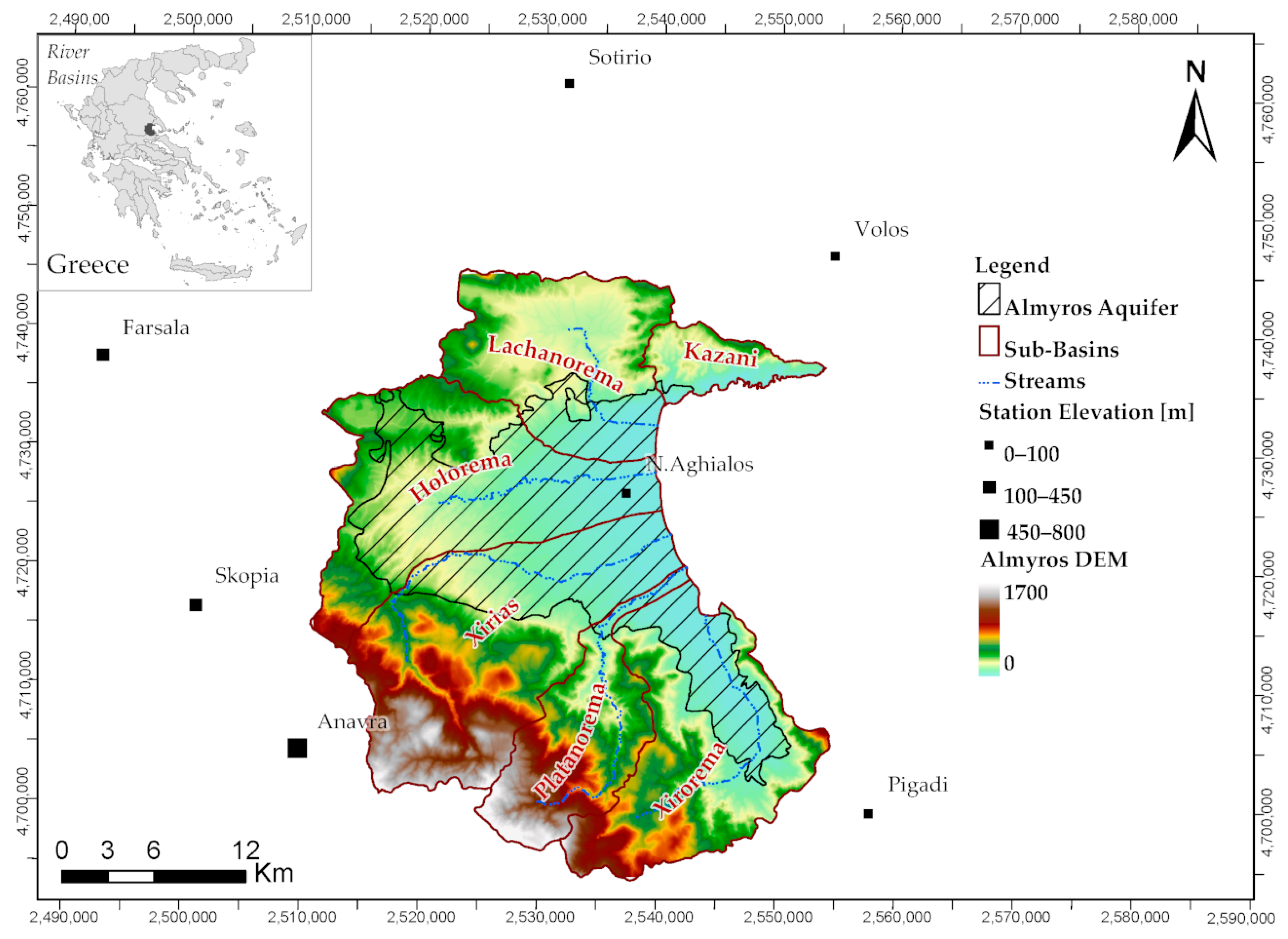
3.1. Study Area

The Almyros basin is located in the central region of Greece, Thessaly. The total area of the basin is approximately 856 km². The geomorphology of the basin is characterized by the presence of ephemeral streams and the absence of surface water storage bodies. It is the only plain of the coastal Thessaly and consists of six sub-basins, namely, Kazani, Lahanorema, Holorema, Xiria, Platanorema, and Xirorema (Figure 2). The basin consists of about 30% plain areas (elevation lower than 150 m), 57% semi-mountainous areas (elevation 150–800 m), and 13% mountainous areas (elevation higher than 800 m). The aquifer covers the lowest and coastal part of the basin and has an area of 293 km² with about 71% of its extent area to be in planar and 29% in hilly terrain. The Almyros basin area is delineated by the Chalkodonion or Mavrovouni mountains in the north and the Othrys Mountain of the Pindus Mountain Range in the west, while the coastline forms the eastern boundary of the Pagasitikos Gulf [82].

The climate of the basin is semi-arid Mediterranean climate with hot and dry summers and cold and wet winters. Mean annual precipitation, for the meteorological station in N.Aghialos, the only station located in the basin (Figure 2), is about 491 mm with a standard deviation of 111 mm, and mean annual temperature is 16.5 °C, with a standard deviation of 0.6 °C. The mean annual precipitation is distributed in time by 12.3% in October, 11.8% in November, 13.4% in December, 9.5% in January, 9.7% in February, 10.3% in March, 6.7% in April, 7.7% in May, 4.5% in June, 3.9% in July, 3.3% in August, and 6.9% in September. The monthly mean temperature varies from the mean annual temperature by 3.3% in October, −26.4% in November, −50.5% in December, −58.9% in January, −51.9% in February, −36.6% in March, −11.2% in April, 20.0% in May, 51.4% in June, 65.0% in July, 60.4% in August, and 35.4% in September.

The basin includes an intensive irrigated agricultural area of about 205 km². The agricultural area mostly covers the area of the aquifer. The main crops cultivated are alfalfa, cereals, cotton, maize, trees, olive groves, vegetables, vineyards, and wheat. The main land uses and the cultivated corps are presented in

Table 1. Percent land use area irrigated by the Almyros aquifer.

Main Land Use/Crop	2010 (% Area)	2018 (% Area)	Irrigation Return Flow Coefficient
Alfalfa	7.74	16.83	0.15
Cereals	10.33	25.16	0.15
Cotton	8.55	8.40	0.20
Maize	2.55	1.62	0.35
Olives	10.86	12.91	0.13
Trees	1.34	2.36	0.13
Vegetables	1.62	6.56	0.24
Vineyards	2.02	2.46	0.13
Wheat	32.75	9.92	0.19

. In the Almyros basin, there is no surface storage project for the storage and use of surface water and all irrigation water demands and urban water supply (and other water uses) are covered by groundwater pumping.

The main soils types in the study basin and, especially, the area of the aquifer are clay loam, clay, and silt loam (

Table 2. Areal percentage coverage of soil types of the Almyros basin according to the U.S. Department of Agriculture (U.S.D.A.) classification.

Soil Texture Class	% Area
Sandy Loam	1.1
Loam	10.4
Silt Loam	21.4
Sandy Clay Loam	2.6
Clay Loam	35.2
Silty Clay Loam	6.5
Sandy Clay	0.2
Silty Clay	1.3
Clay	21.3
Sandy Loam	1.1

). Most of the materials are alluvials deposited in the middle and low elevation areas of the basin by the streams and torrents of the area. The hydrological soil group of type B (medium low runoff potential when saturated), based on data from the previous study of Thessaly [1], covers the 254 km² of the overlaying aquifer area, while soil groups A (low runoff potential when saturated), C (medium high runoff potential when saturated), and D (high runoff potential when saturated) occupy 12.3 km², 7.3 km², and 19.1 km², respectively.

The coastal low-land area of the basin mostly comprises of sandy permeable materials with clay lenses. Clay layers and the intercalations of clay, sand, gravel with volcanic rocks and conglomerates, form low permeability structures in the western area and higher elevation areas of the basin. In the southern part of the basin, small areas of limestone form kasts, which are direct communication with the sea [82]. The geological and hydrogeological setting of the study area and the relative data are presented in the Section 3.2.4 of the paper and in Figure 3.

3.2. Database

The simulation of water resources requires databases of a wide range of measured variables that span over many years of monitoring for calibration and validation purposes of the models. Climatic variables (e.g., precipitation and temperature), water table measurements of wells, and groundwater nitrates and chloride concentrations were also required and used in the analysis. Land use and crop type data were used to estimate the crop irrigation demands, number, and groundwater well abstractions.

3.2.1. Meteorological Data

Monthly precipitation and temperature collected in six (6) meteorological stations distributed in and around the basin were used in this study. The locations of the stations are depicted in Figure 2. The range of the elevation of the stations is among 3 m and 850 m. Daily and monthly precipitation data, daily and monthly minimum, maximum and mean temperature data were available for the station of N.Aghialos, the only station located in the basin, from 1961 to 2018. The meteorological data are collected by various governmental organizations and agencies. They have been pre-processed and validated.

3.2.2. Land Use

The agricultural land use occupies almost 70% of the aquifer area for the historical period. The spatial distribution of the cultivated fields across the aquifer counties was provided for the years 2010 and 2018, by the Greek Payment Authority of Common Agricultural Policy (C.A.P.) Aid Schemes (OPEKEPE). The crop data were grouped into nine main crop categories. Thus, the main crops cultivated in the aquifer area are alfalfa, cereals, cotton, maize, trees, olive groves, vegetables, vineyards, and wheat. The irrigation return flow was estimated with irrigation return coefficients as measured in fields with similar soil characteristics and climatic conditions, for every main crop category [83,84,85]. The distribution of the main crop categories for the years 2010 and 2018, and the respective irrigation return flow coefficients are shown in Table 1.

Moreover, crop yield data are publicly available by the Greek Payment Authority of Common Agricultural Policy (C.A.P.) Aid Schemes (OPEKEPE). The crop yield data span from 2000 to 2018 and refer to annual measured crop yields for various crop types.

3.2.3. Soil Characteristics of Unsaturated Zone

Soil physical and hydrological parameters of saturated conductivity, bulk density, soil water content at the wilting point, and field capacity, organic carbon concentration, exchangeable K concentration, electrical conductivity, and initial water storage were provided from European Soil Data Centre (ESDAC) [86,87]. The sand, clay, and silt content, and coarse fragments were estimated from point observation data provided by (OPEKEPE) and National Agricultural Research Foundation (NAGREF). According to the U.S. Department of Agriculture (U.S.D.A.) soil texture classification [88] the soils overlaying the Almyros aquifer are classified and presented in Table 2.

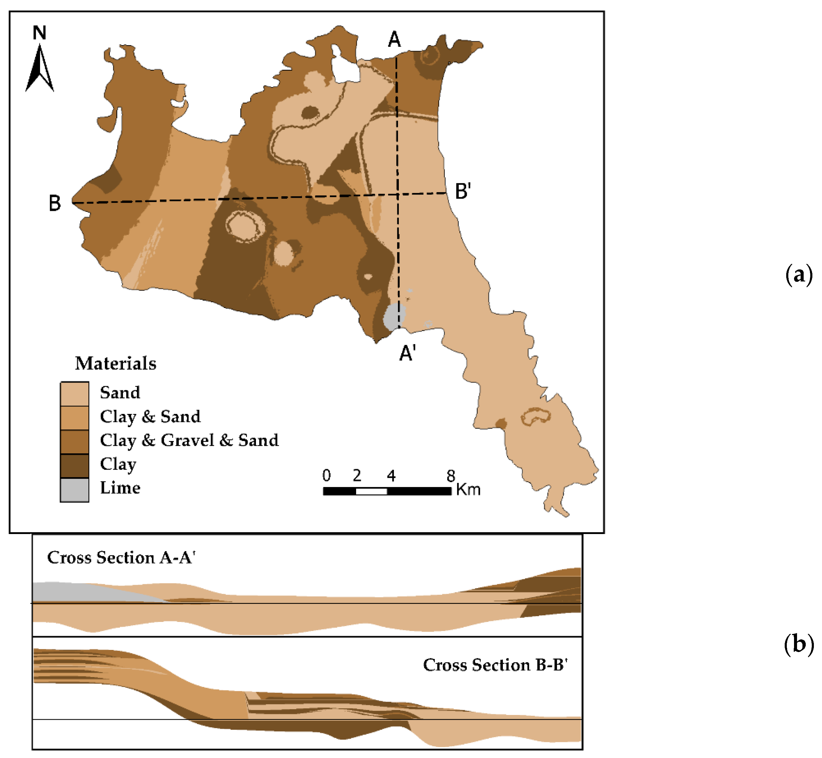
3.2.4. Geology and Hydrogeological Setting and Data

The coastal low-land area consists mostly of sandy permeable materials with clay lenses towards the western part of the basin, following the topographical elevation change. In the western and high elevation areas of the basin and the aquifer, the presence of a low permeability clay layers and the intercalations of clay, sand, gravel with volcanic rocks and conglomerates, form low permeability structures within the granular aquifer. Limestone is present at small areas of the southern part of the basin and the aquifer area, forms karsts, which are in direct communication with the sea and do not interact with the aquifer [82]. No significant hydraulic communication has been observed and documented for the northern, western, and southern part of the aquifer with the neighbouring aquifer systems.

Borehole data of 55 wells in the area of Almyros drilled between 1968 and 1990, from the Greek Ministry of Agriculture, were used to produce the stratigraphy of the aquifer. The main geological materials of the Almyros aquifer are classified into five categories, namely clay (Neogene), clay-gravel-sand (Neogene), sand (Quaternary), clay-sand (Neogene), and limestone and form the aquifer of the study basin. The top view and the two most representative cross-sections of the geological materials of the aquifer are presented in Figure 3.

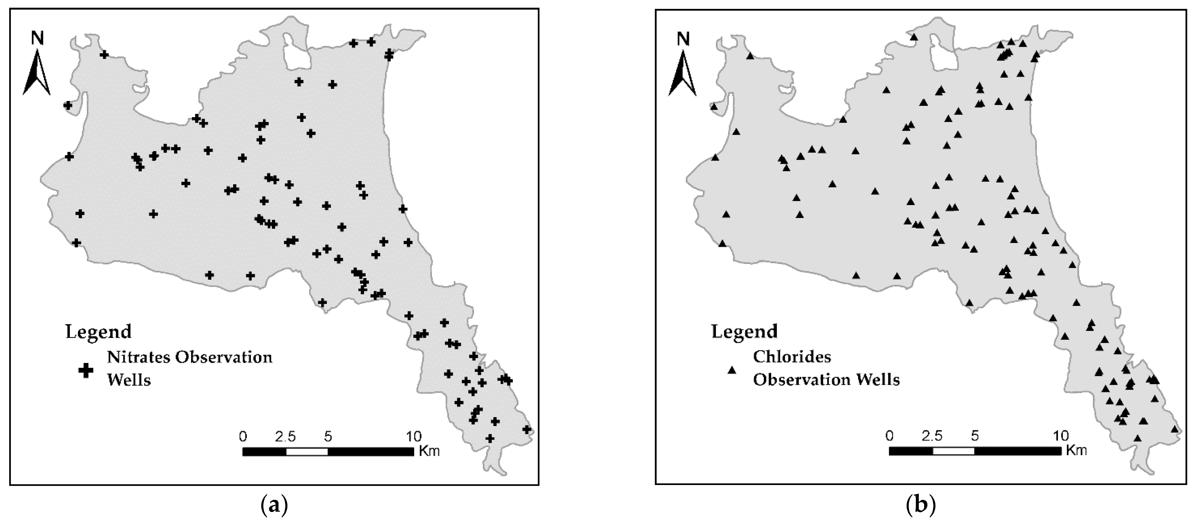
3.2.5. Observation Data of Water Table, Nitrate Concentrations, and Chloride Concentrations

Well observation data regarding the water table, the nitrates concentrations, and the chloride concentrations were mostly performed and provided by the Institute of Geology and Mineral Exploration (IGME), the Regional Government of Thessaly, and the Magnesia Prefecture. The measurements span from 1991 to 2015. Additional nitrates concentrations measurements and chloride observation measurements for the period of 2013 to 2015 were performed in the Almyros aquifer, in a previous research study [82]. The locations of water table observation wells are illustrated in Figure 4a. Known locations of pumping wells were extracted by regional well maps and the National Register of Water Abstraction Points from Surface and Underground Water Bodies [89]. The distribution of pumping wells is presented in Figure 4b.

The distribution of wells of observed nitrates concentrations and chloride concentrations are presented in Figure 5a,b, respectively.

4. Results

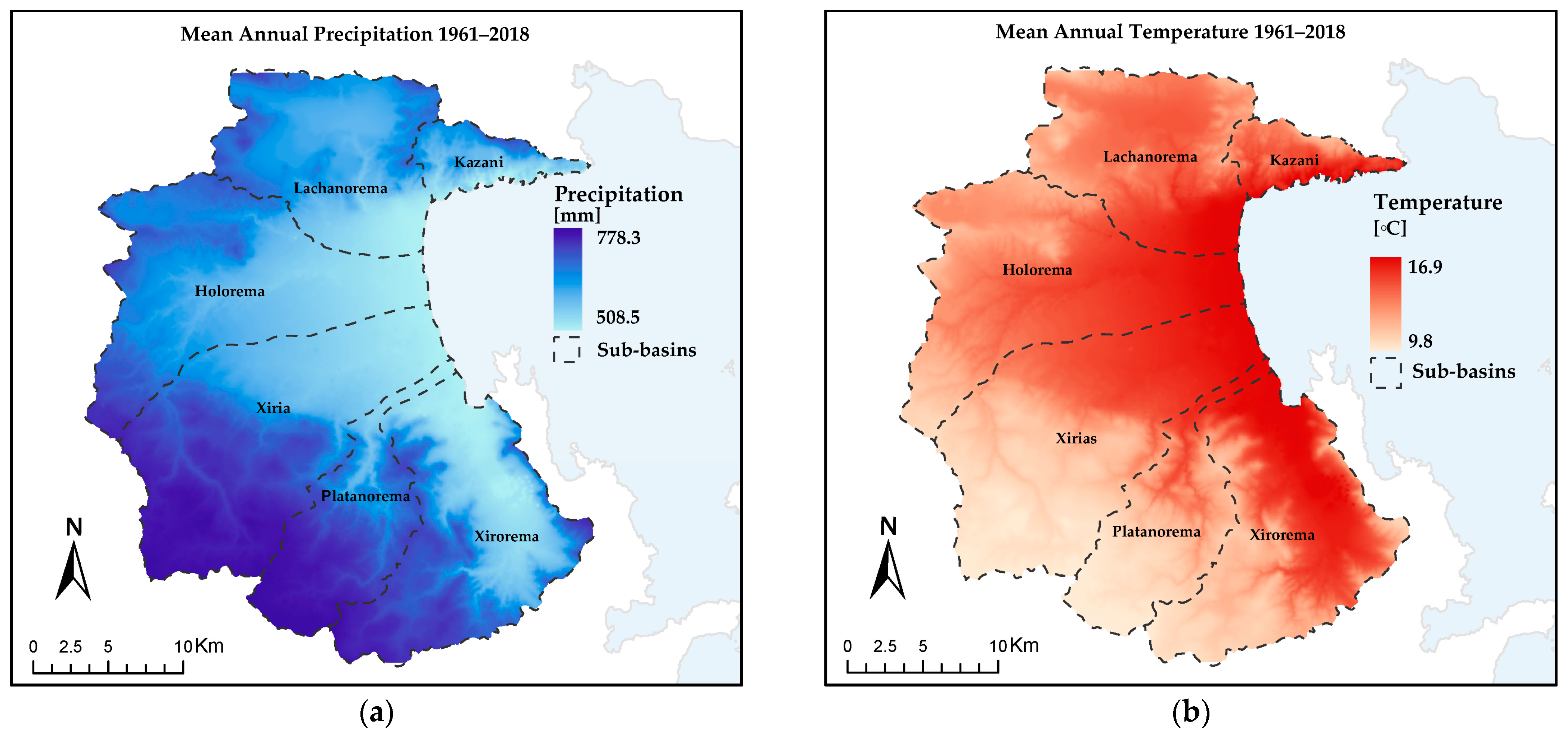
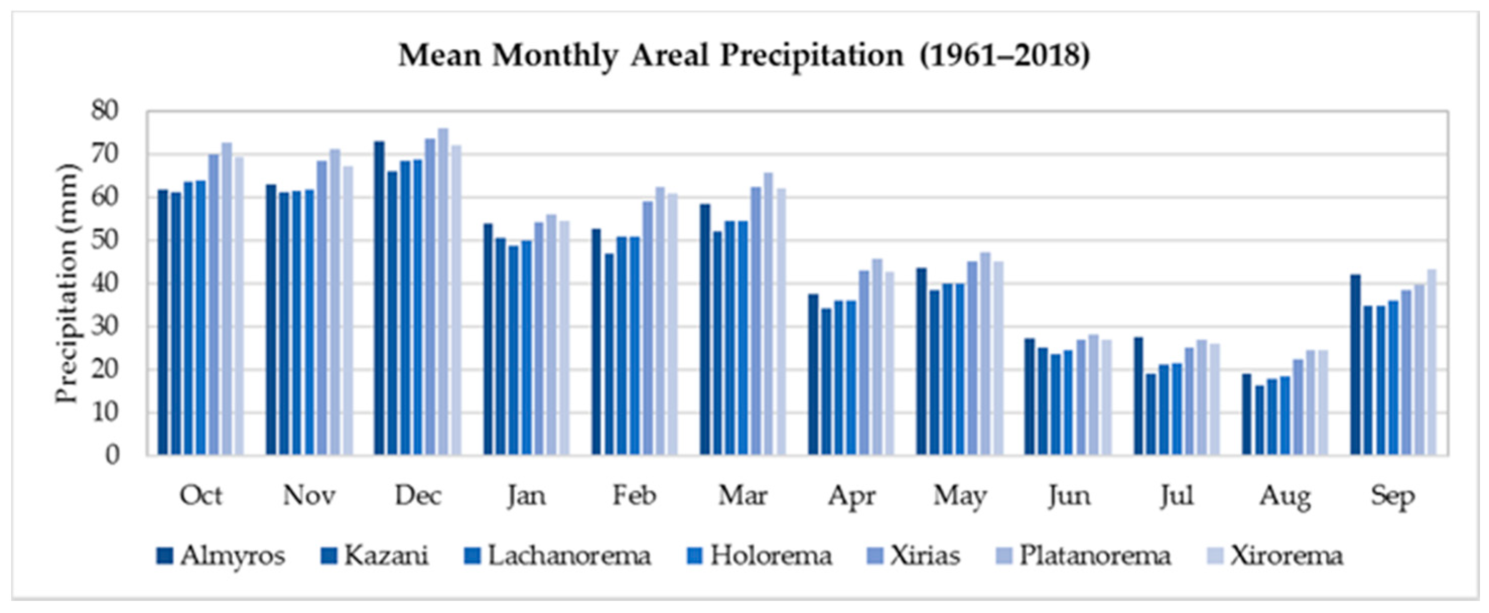
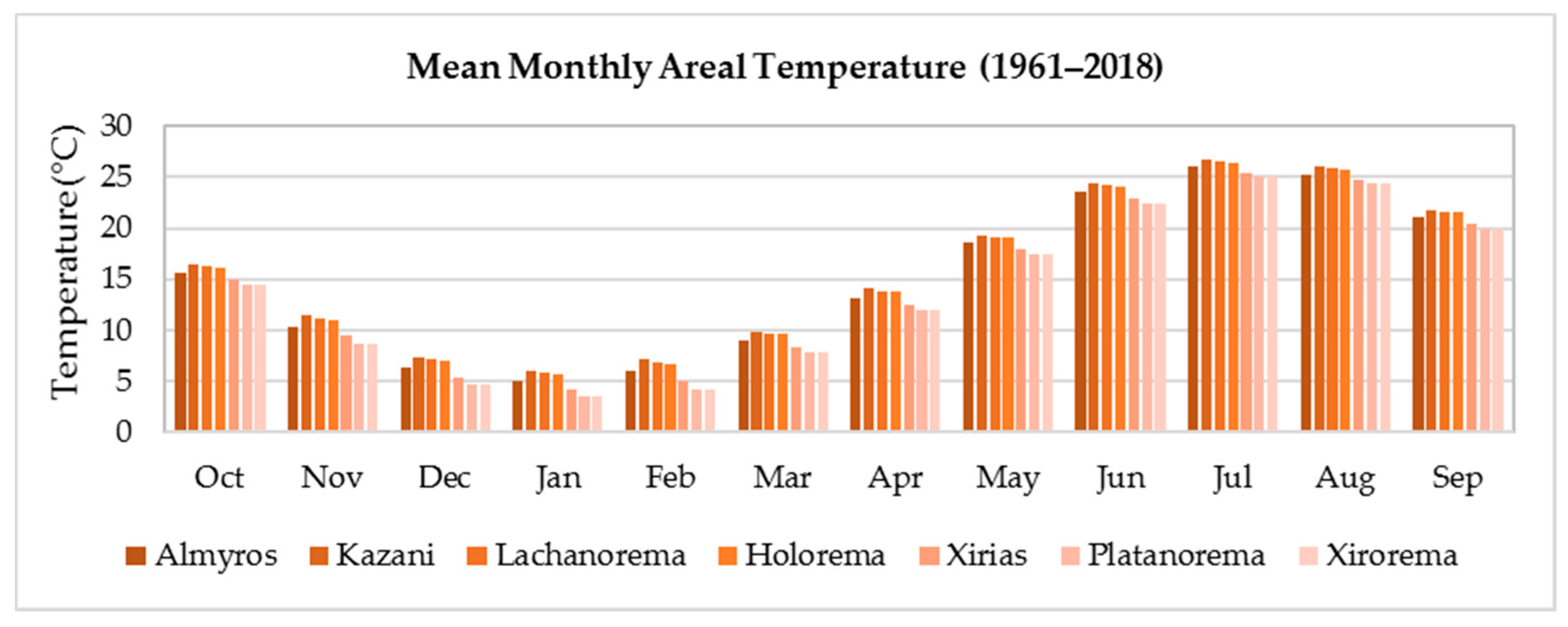
4.1. Mean Areal Precipitation and Temperature

The daily meteorological data of the station in N.Aghialos were aggregated to produce monthly time-series of the variables of precipitation and temperature. The precipitation and temperature missing data of the surrounding stations were infilled using linear regression based on the N. Aghialos station, the only station in the region with no missing values. The coefficients and correlation of the stations used for the estimation of precipitation and temperature are shown in

Table 3. Linear regression coefficients of the stations for the precipitation variable.

Precipitation Station	Slope	Intercept	R2	R
N. Aghialos	1.00	1.00	1.00	1.00
Anavra	0.93	15.49	0.74	0.86
Skopia	0.96	6.71	0.69	0.83
Volos	0.99	0.00	0.90	0.95
Pigadi	0.90	10.43	0.65	0.80

and

Table 4. Linear regression coefficients of the stations for the temperature variable.

Temperature Station	Slope	Intercept	R2	R
N. Aghialos	1.00	1.00	1.00	1.00
Pigadi	0.84	2.94	0.16	0.40
Volos	0.93	2.12	0.29	0.54
Skopia	0.97	−1.10	0.37	0.61
Sotirio	0.11	1.00	0.40	0.63
Farsala	0.83	−0.86	0.42	0.64

.

For the estimation of areal precipitation, the gradient method modified with the Thiessen polygon method was used. The gradient for the annual precipitation to 100 m of elevation change in the Almyros basin is 15.9 mm (R² = 0.70), while the gradient for the annual temperature is −0.43 °C per 100 m increase in elevation for the whole basin (R² = 0.71). The spatial distribution of mean annual precipitation and temperature is presented in Figure 6.

The monthly mean areal precipitation was estimated with the use of the gradient method and the Thiessen polygon method per-sub-basin. The mean annual precipitation of the Almyros basin has an average of 566 mm, a median value of 540 mm, and a standard deviation of 107.16 mm. The driest year with the least annual precipitation that exceeds more than 40% of the interannual average is the hydrological year of October 2006 to September 2007 with 355.9 mm annual precipitation. The wettest years with more than 40% exceedance from the average value are the hydrological years of 1968–1969, 1981–1982, 2002–2003, and 2017–2018. The monthly mean areal temperature was estimated with the gradient method. The mean annual temperature of the Almyros basin has an average of 15.0 °C, and a standard deviation of 0.64 °C. The hottest monthly areal temperatures were noted in July 1988 with 28.1 °C, in August 2010 with 28.6 °C, and in July 2012 with 28.8 °C at the mean elevation of the Almyros basin.

Mean annual areal precipitation for the simulation period of October 1991 to September 2018, is estimated at 561 mm and mean annual areal temperature is estimated at 15.41 °C. The monthly averages of areal precipitation and temperature are presented in Figure 7 and Figure 8.

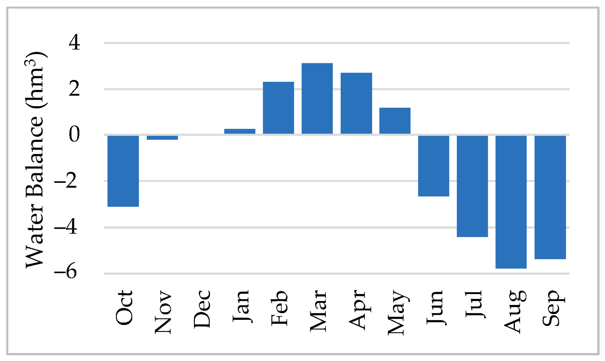
4.2. Surface Hydrology-Groundwater Recharge

The UTHBAL model simulated the monthly surface hydrologic balance of the Almyros basin from October 1960 to September 2018. It was not possible to calibrate the model in the sub-basins of the Almyros basin because there are no streamflow measurements of the Almyros ephemeral stream discharge. For these reasons, most of the parameters of the model were taken the values found in a regional analysis of the model in Thessaly [28]. The values of the model used in the study were: the parameter of monthly melt rate factor, Cm= 6 mm/°C, the coefficient of actual evapotranspiration, α= 0.48, the coefficient of interflow β = 0.033, the coefficient of baseflow, γ= 0.203, and the coefficient of groundwater recharge, K = 0.68. The parameter of the Curve Number, of the US Soil Conservation Service [48] was estimated for each sub-basin with the HEC-GeoHMS tool in ArcGIS [90], based on soil type (A, B, C, D) maps, Corine Land Cover uses, and the Digital Elevation Model of the area. The weighted average Curve Number per sub-basin is shown in

Table 5. Curve Number of the Almyros basin and its sub-basins.

Basin	CN
Almyros	61.43
Kazani	67.93
Lahanorema	68.11
Holorema	68.47
Xirias	60.69
Platanorema	51.07
Xirorema	53.84

.

The mean annual surface runoff is 113.49 mm and the median annual surface runoff is 106.11 mm, found for the year 1999–2000. The wettest year with the largest cumulative annual runoff is 1962–1963, and the driest year with the least cumulative annual runoff is 2004–2005. The mean annual groundwater recharge is 54.1 mm for the whole basin. The wettest year is 1962–1963 with 214.4 mm. The median of the simulated years is noted in 2003–2004 with 43.2 mm of recharge, while the driest year is encountered in 2004–2005, with 0 mm of groundwater recharge. Interannual statistics of the simulated runoff, recharge, and precipitation to the input water of the region are depicted in

Table 6. Mean annual statistics of precipitation (P_b), surface runoff (Q_c), and groundwater recharge (R_g) per sub-basin for the period of October 1961 to September 2018.

Sub-Basin	Pb [mm]	Qc [mm]	Rg [mm]	Qc/Pb	Rg/Qc	Rg/Pb
Kazani	507.9	97.5	56.3	19.2%	57.7%	11.09%
Lachanorema	522.8	103.6	62.5	19.8%	60.4%	11.96%
Holorema	527.9	105.5	65.1	20.0%	61.7%	12.33%
Xirias	590.4	125.4	63.5	21.2%	50.7%	10.76%
Platanorema	617.8	127.46	34.2	20.6%	26.8%	5.54%
Xirorema	596.6	112.4	31.9	18.8%	28.4%	5.35%

.

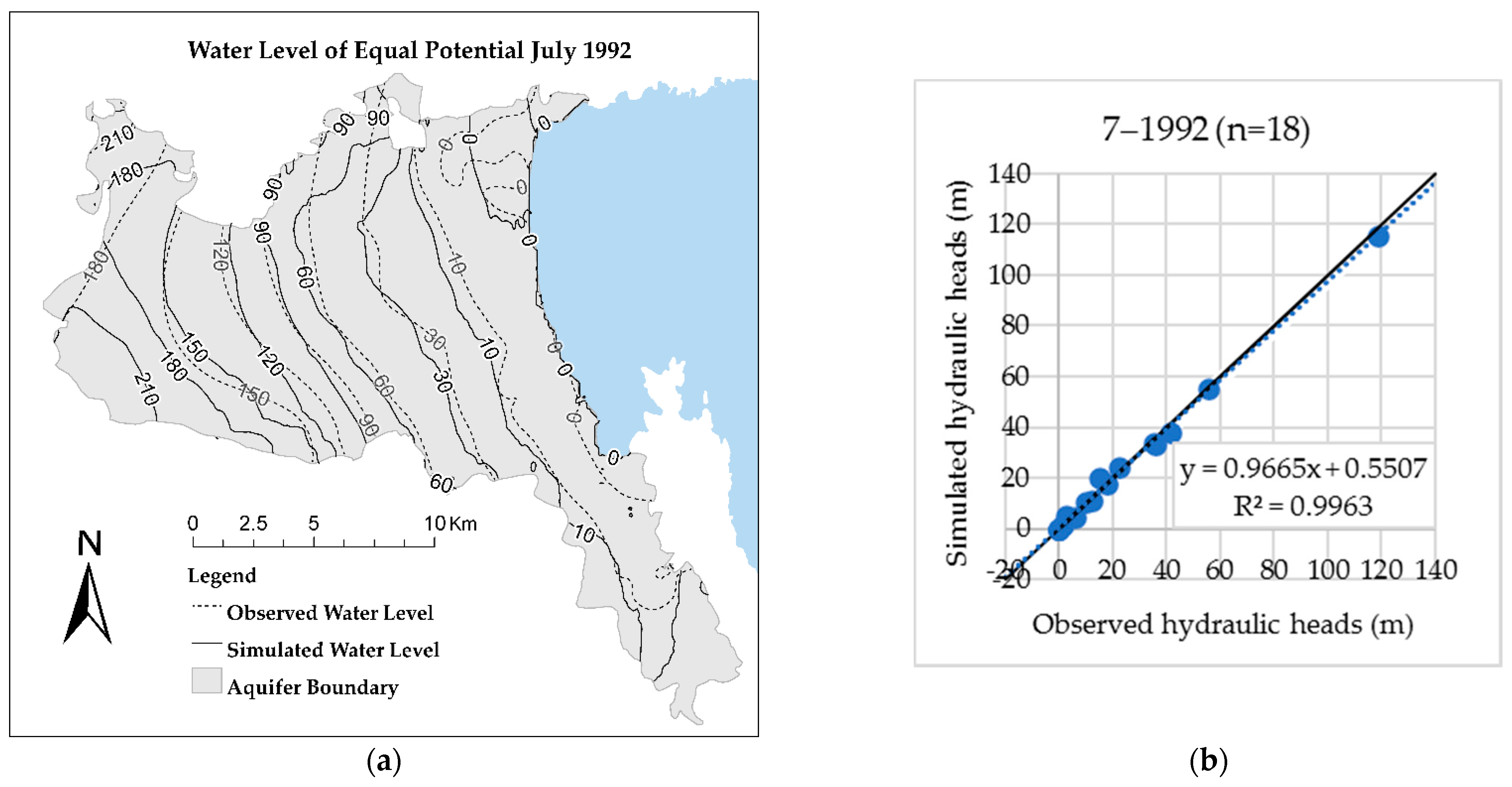
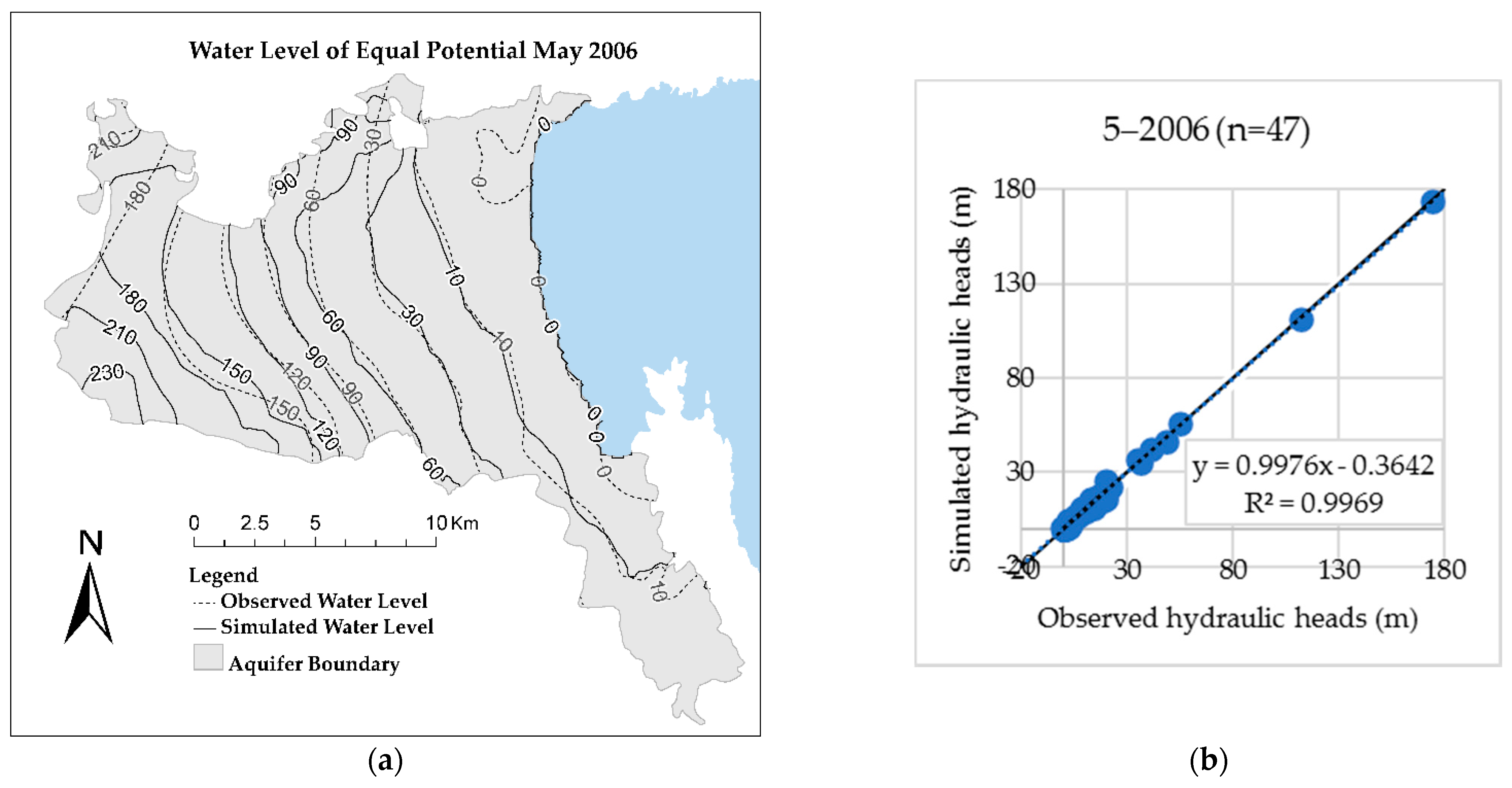
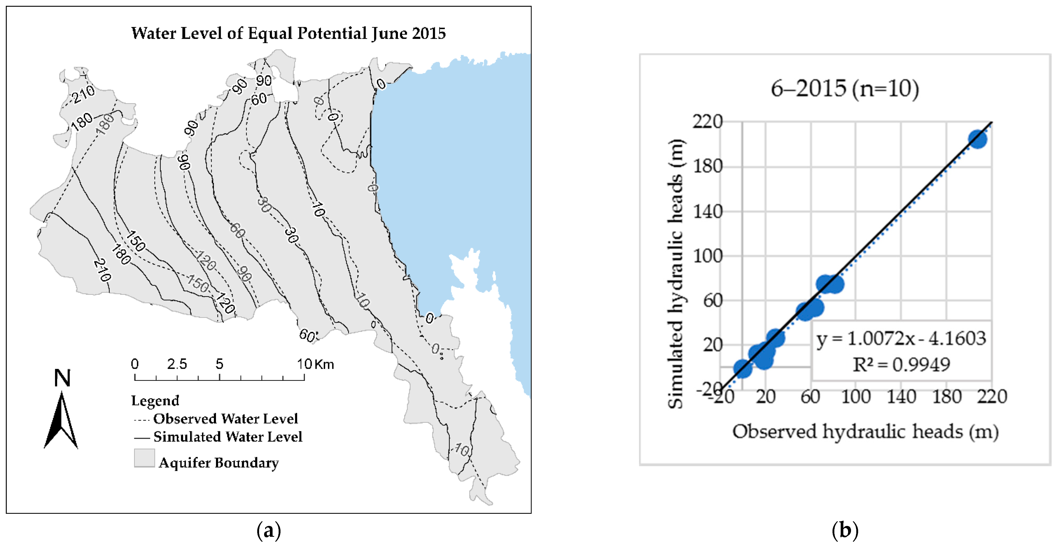
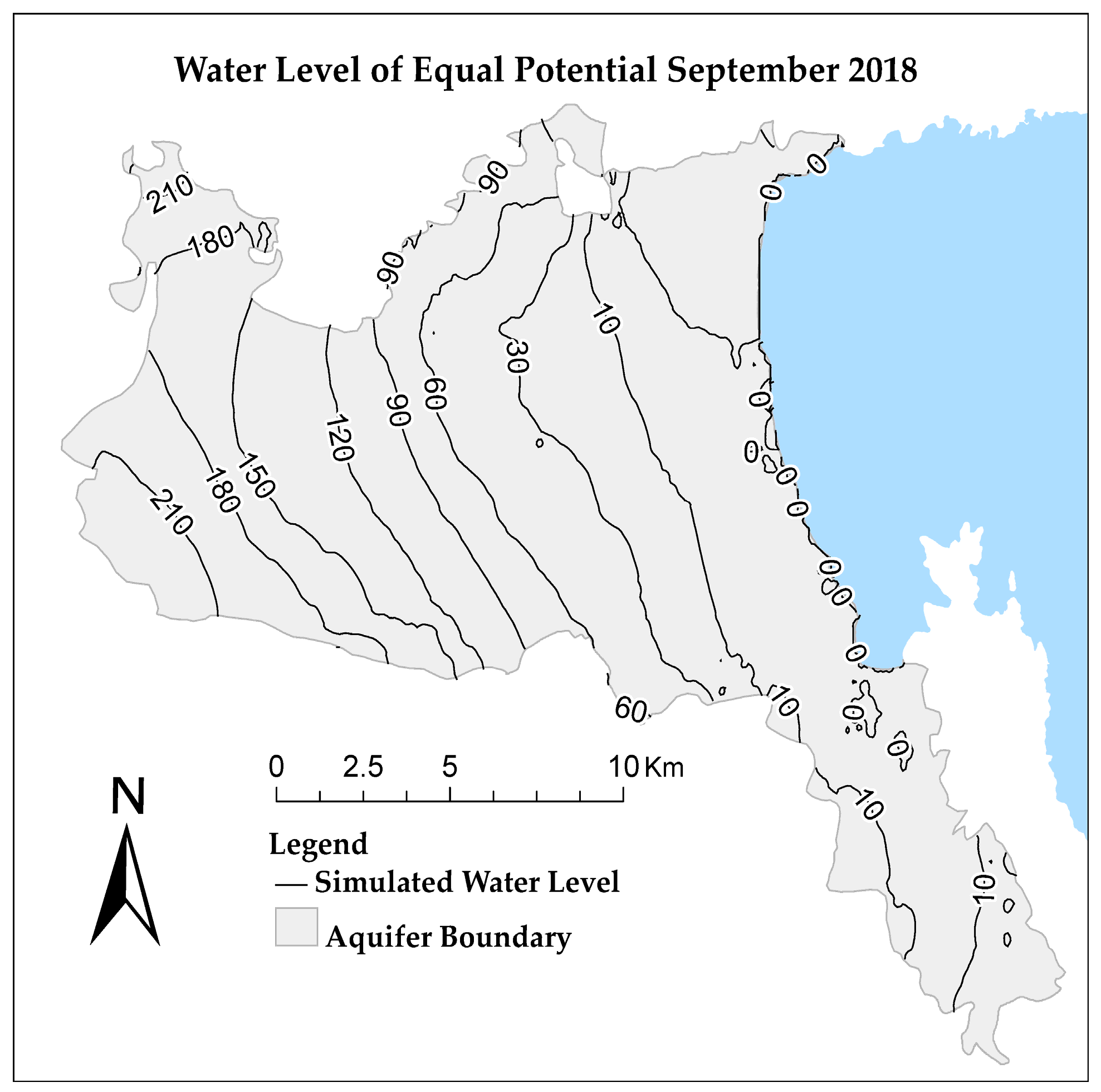
4.3. Ground Water Flow

The MODFLOW model simulated the groundwater recharge, the well abstractions, the change of the storage of the aquifer, and the sea fluxes to the coastline, in a monthly transient mode, for the period of October 1991 to September 2018. The water table observations of 75 wells were used for the definition of the starting heads of the aquifer in October 1991, as well as, for the calibration and the validation of the model.

The model discretization forms a one-layer rectangular grid of 200 rows and 200 columns, with a cell size of approximately 150 m × 150 m and consists of 40,000 cells with 12,464 of them being active. Unconfined conditions were considered for the simulation of the aquifer with the Layer Property Flow package. The coastline at the eastern part of the aquifer was considered as a Constant-Head-Boundary, at zero m above sea level. In the western part, the boundary condition was set a No-Flow Boundary, according to the imperviousness of the adjacent geological formations at the margins of the aquifer. The hydraulic conductivity was simulated in zones, according to the hydrogeological characteristics of geological formations. In particular, the number of simulated water abstraction wells was estimated at 2072 wells, 28 of which are urban water supply wells and 2044 are irrigation wells. The estimated pumping rates were based on the water demands of crops and the water losses of the local irrigation private-owned systems. The crop water demands were estimated with the Near Irrigation Requirement (NIR) method [91] and are distributed in the sub-basins, on average, by 9% in Kazani, 20% in Lahanorema, 21% in Holorema, 19% in Xirias, 17% in Platanorema, and 14% in Xirorema. The averaged water losses of the irrigation systems are equal to 41% of the crop water demands, according to [28]. Measured pumping rates per county were also compared against the estimated pumping rates.

The model was calibrated for the period October 1991 to September 2009 and validated for the period October 2013 to September 2015. Calibration was performed using PEST for the coastal and central part of the aquifer, based on available hydraulic conductivity measurements of several boreholes, mostly located in the coastal region. The values of horizontal anisotropy, specific yield, specific storage, and the upland hydraulic conductivity were kept at the values set by the previous simulation of the Almyros groundwater flow [28]. Sensitivity analysis indicated that the most sensitive hydraulic conductivities of the hydrogeological formations are located in the Xirias and Xirorema sub-basin. Specifically, the sensitive regions are (i) in a very small area of hydraulic conductivity of 0.05 m/day, consisting of marl and lignite compounds, (ii) along the southern semi-mountainous boundary of Neogene formations with 1.0 m/d, (iii) the upper part of Xirias sub-basin consisting of calcareous conglomerates with 0.8 m/d, and (iv) the eastern alongside Neogene formations of Xirorema sub-basin with 1.2 m/d. Groundwater flows from the western higher part of the aquifer towards the low elevation eastern coastal region and higher velocities are encountered in the central Holorema and Xirias sub-basin following the distribution of hydraulic conductivity. The values of hydraulic conductivity range between 0.1–18.7 m/day, with a spatial average value of 2.3 m/d with the highest value encountered in the north-eastern part of the aquifer near the coastline. The calibration results for the groundwater model indicate that the Nash–Sutcliffe model efficiency, the Pearson correlation, and the Index of Agreement are, on average, for the simulation period 0.986, 0.989, and 0.996, respectively. Summary statistics for the calibration and the validation period are depicted in

Table 7. Summary efficiency statistics of the MODFLOW model.

MODFLOW	Calibration Average 1991–2009	Validation Average 2013–2015
Eff	0.975	0.997
R2	0.981	0.997
IA	0.993	0.999

.

Simulated contours of the water table of equal potential against the respectively observed contours are presented for July 1992, September 2006, and June 2015 in Figure 9, Figure 10 and Figure 11. The simulated water table at the end of the simulation period in September 2018 is presented in Figure 12. The simulated water table contours are almost identical to the observed water table contours. Additionally, scatterplots of the simulated water head of wells against their observed water head have been plotted and the slope and intercept of the regression lines against the slope of the line of perfect agreement (1:1 line has been tested using the t-test).

For July 1992, two-sided t-test was performed for 18 water table wells. The slope and the intercept do not differ significantly from the line of perfect agreement (1:1 line) at α = 0.05 significance level.

For May 2006, two-sided t-test was performed for 47 water table wells. The slope and the intercept do not differ significantly from the line of perfect agreement (1:1 line) at α = 0.05 significance level. For June 2015, two-sided t-test was performed for 10 water table wells. The slope and the intercept do not differ significantly from the line of perfect agreement (1:1 line) at α = 0.05 significance level.

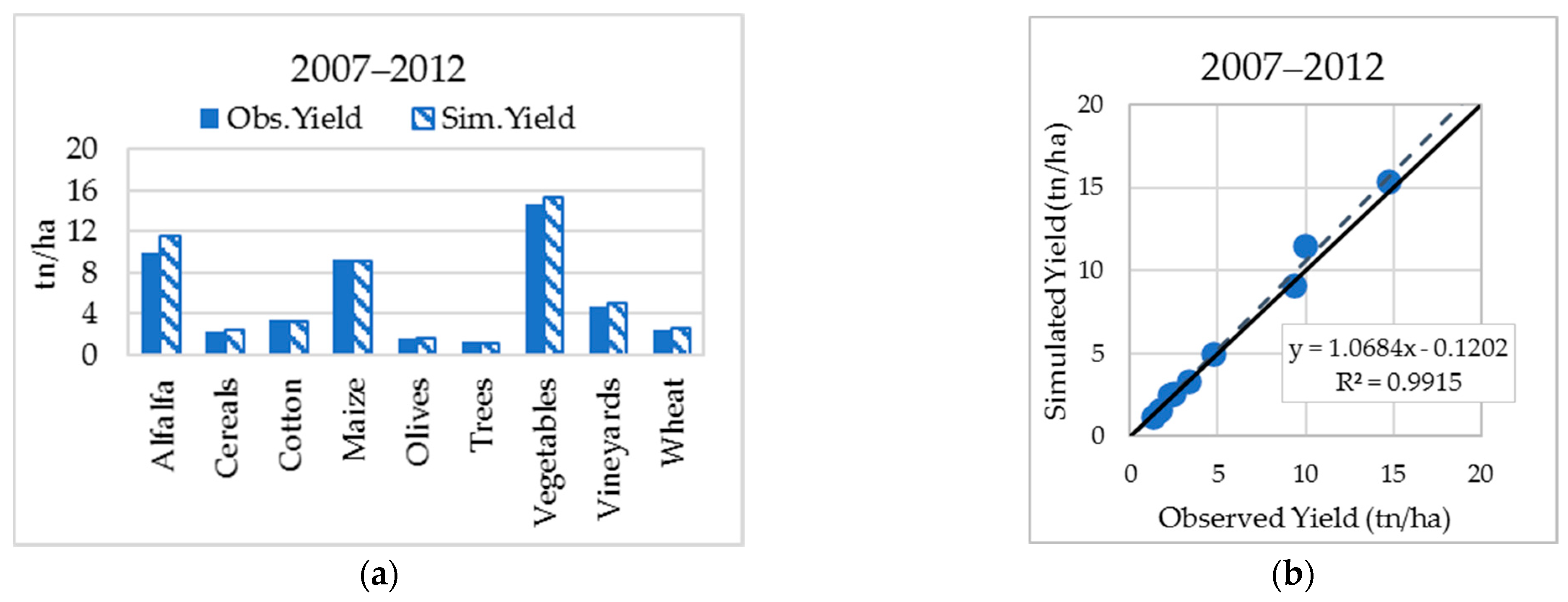
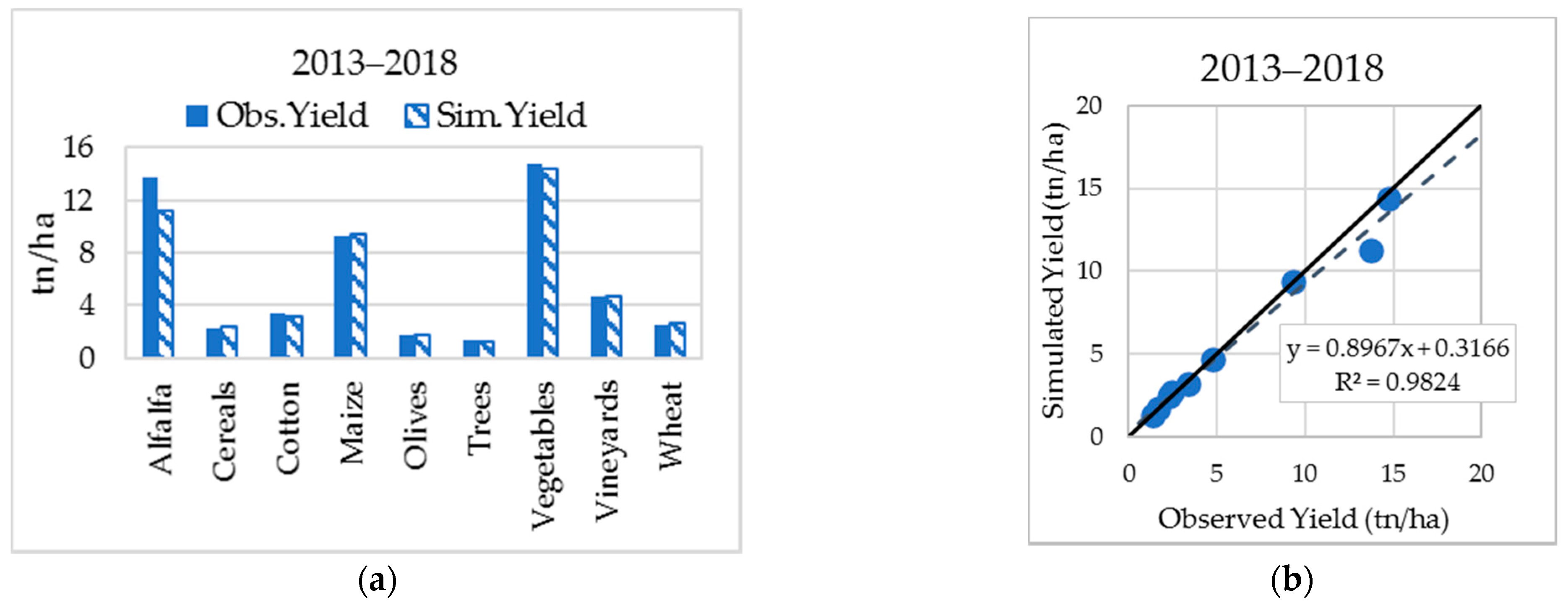
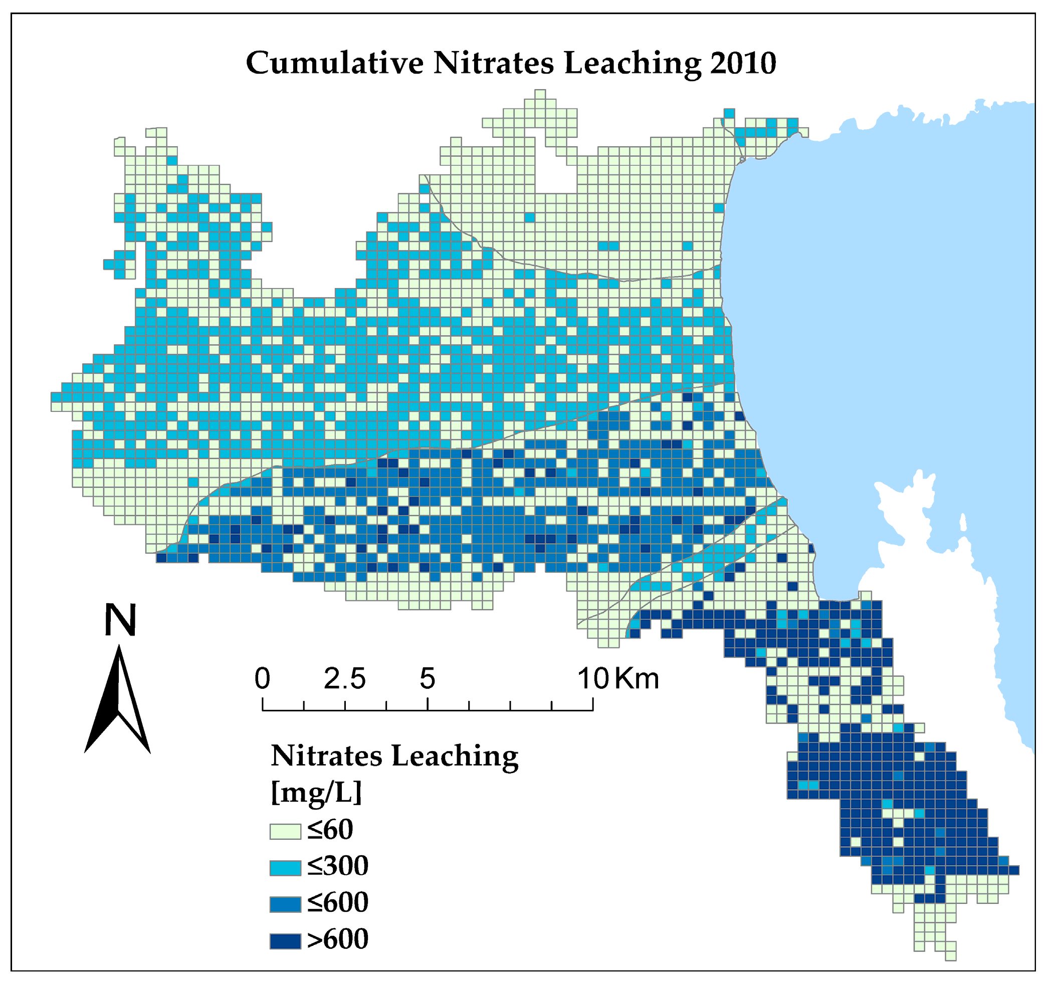
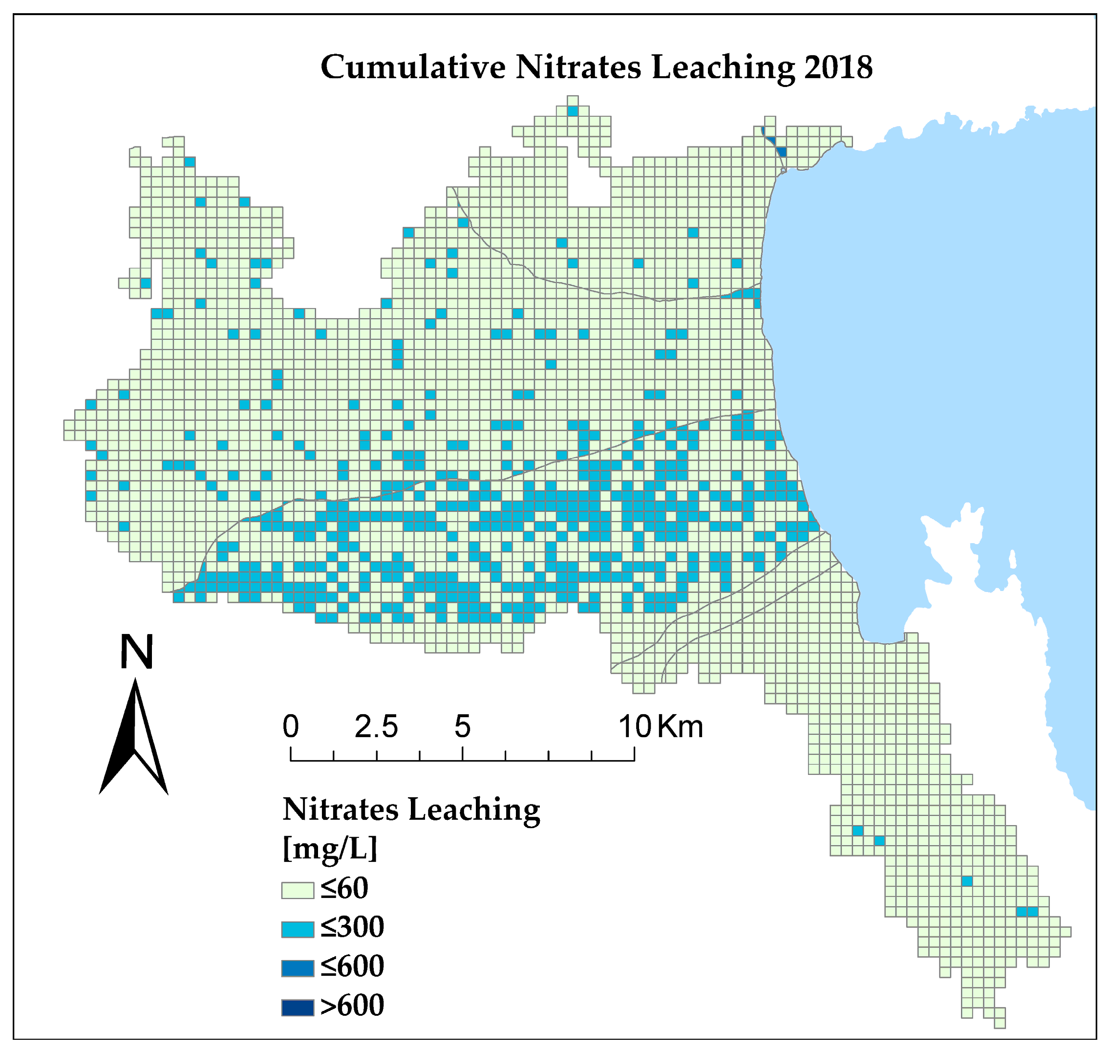
4.4. Nitrate Leaching Simulation

The discretization of the REPIC forms a grid of rectangular cells of approximately 300 m × 300 m and it consists of 3215 cells with one REPIC cell equal to four MT3DMS cells. The nitrates leaching into the Almyros aquifer from the fertilization practices [92] for crop growth were simulated for the stress period of October 1991 until September 2018 with the REPIC model. The simulation took place for four land use periods 1990–2000, 2001–2006, 2007–2012, and 2013–2018 for the main crop types of Almyros. The crop water requirements and fertilizer application are presented in

Table 8. Maximum annual Near Irrigation Requirement (NIR) and typical nitrogen fertilizer loading.

Crop	NIR [mm]	NFer [Kg/ha]
Alfalfa	893	30
Cereals	336	100
Cotton	409	140
Maize	389	325
Olives	515	125
Trees	515	175
Vegetables	271	150
Vineyards	297	125
Wheat	336	160

.

Since there are no nitrate leaching observations of the unsaturated zone of the Almyros basin, the crop growth parameters were calibrated and validated against crop yield data for the periods of 2007–2012 and 2013–2018, respectively. Moreover, the model’s recharge is calculated with a stochastic estimation of the Curve Number and the water balance parameters of the model were calibrated against the sum of recharge, as calculated by UTHBAL, and irrigation return flow. The calibration and validation procedures were performed with R-script in R-studio for each sub-basin for groundwater recharge, and, similarly, for the Almyros basin as a whole, for crop yields. Firstly, vectors of parameters were defined, secondly, a matrix of all their possible combinations was constructed, and then the model was run iteratively, while the code estimated the Nash–Sutcliffe efficiency and R-squared between the simulated and observed crop yields and groundwater recharge values. The parameters that resulted in the best statistical efficiency were considered the appropriate values of the REPIC model for the Almyros basin. Column diagrams of crop yields per crop type combined with the respective scatterplot of simulated crop yields against observed crop yields for the calibration period 2007–2012 are shown in Figure 13 and for the validation period in Figure 14. The slopes and the intercepts of the regression lines of the crop yield scatterplots do not differ significantly from the line of perfect agreement (1:1 line) at α = 0.05 significance level using the two-sided t-test. The average values of statistical measures of efficiency, Nash–Sutcliffe, and R-squared, for the calibration and validation of the simulated crop yields, are shown in

Table 9. Summary efficiency values of simulated against observed crop yields.

Crop	Calibration Average 2007–2012	Validation Average 2013–2018
Eff	0.98	0.92
R2	0.99	0.96
IA	0.99	0.99

. The distributed nitrates leaching maps for the years 2010 and 2018 are depicted in Figure 15 and Figure 16, respectively.

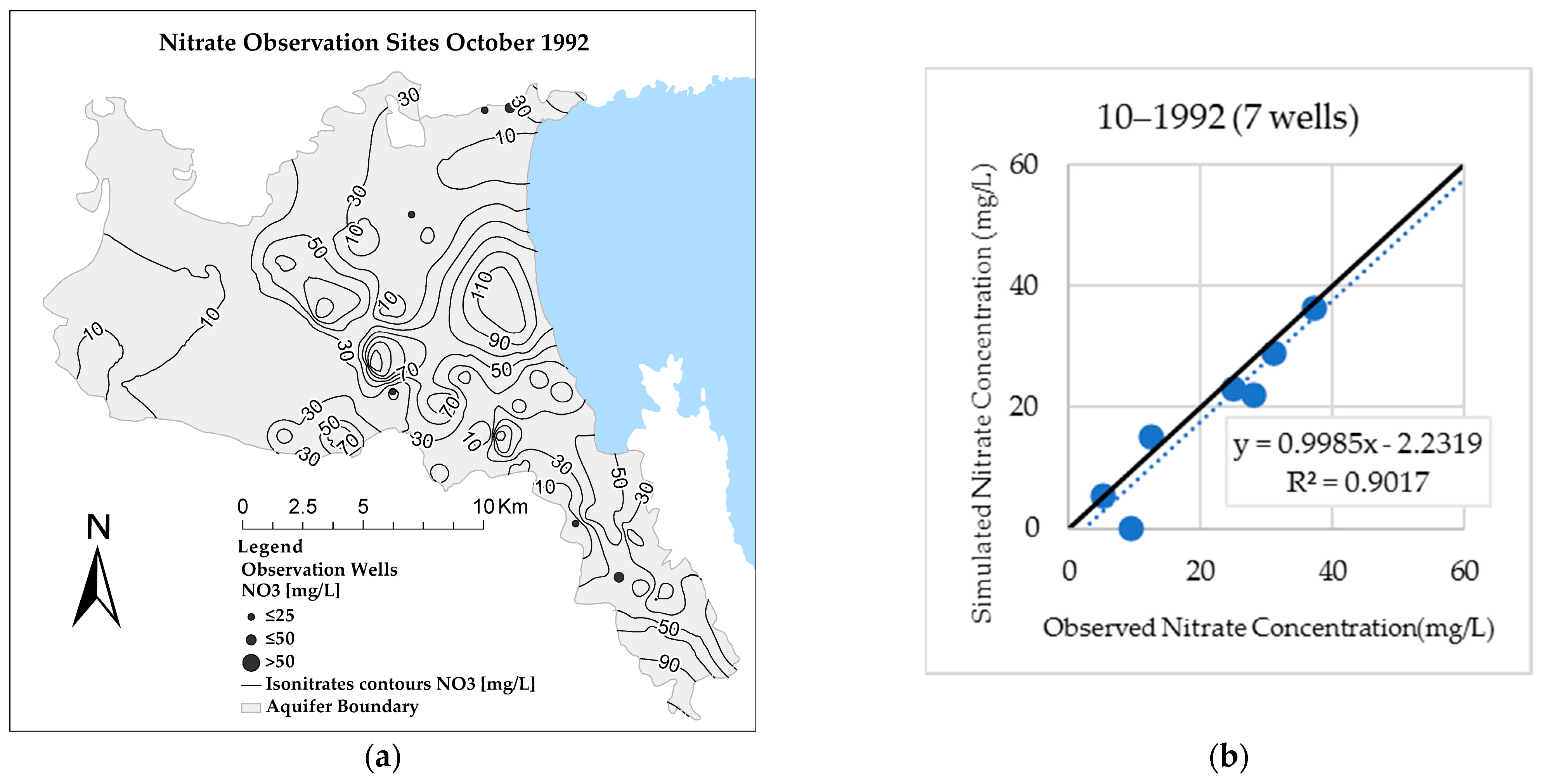
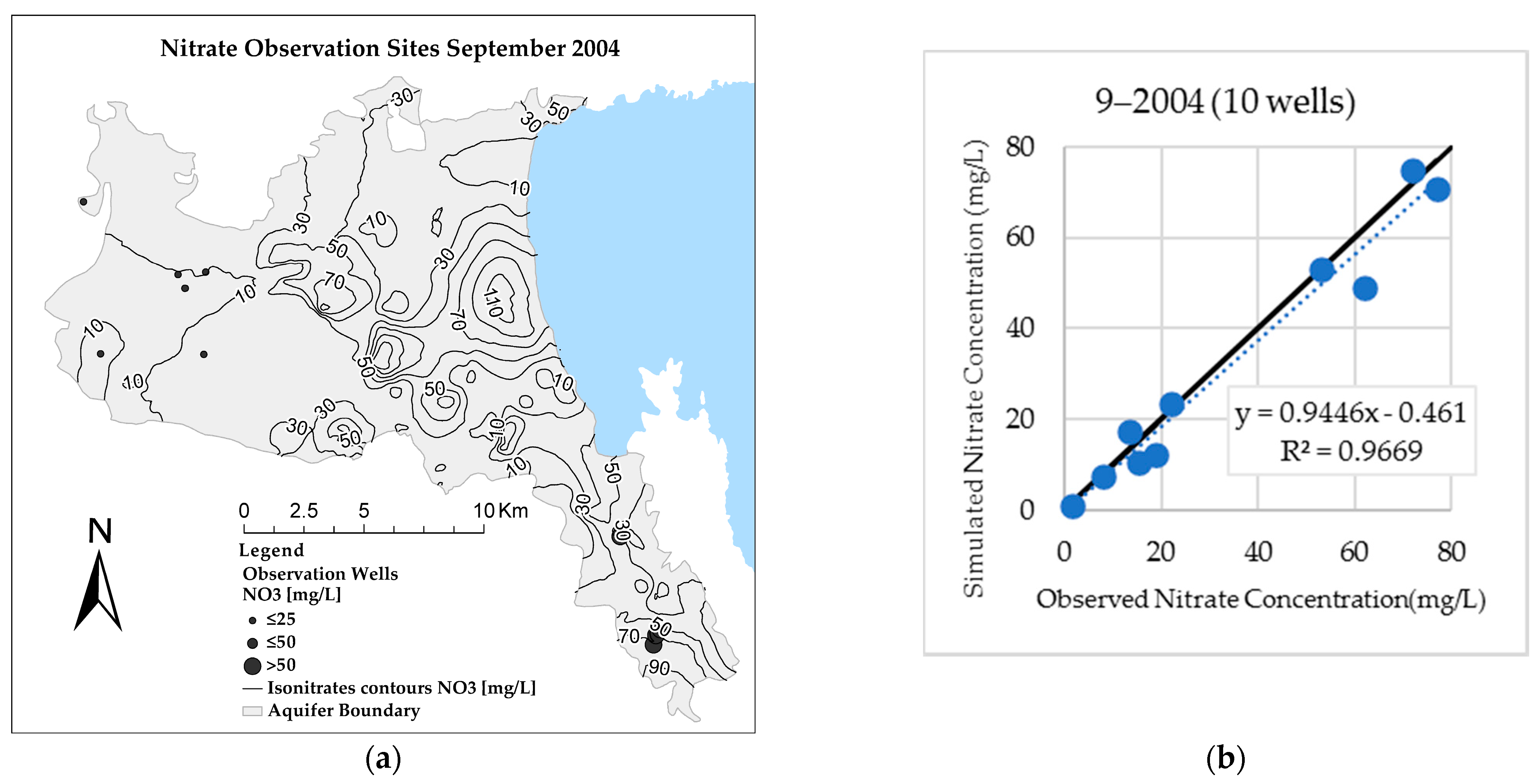
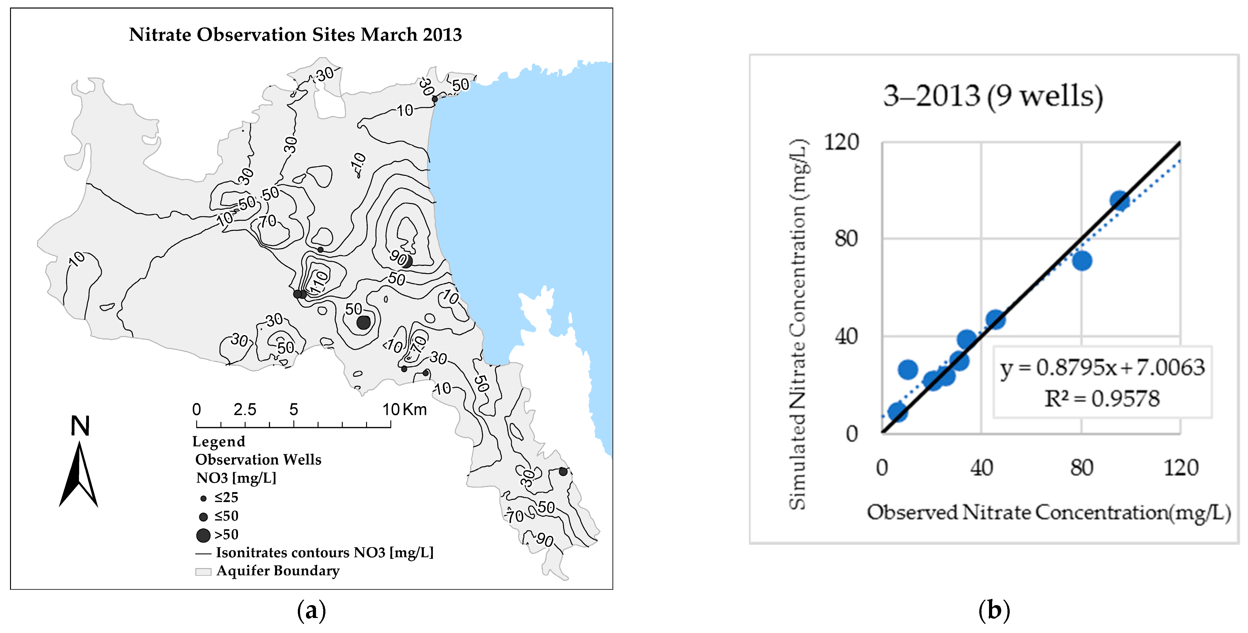
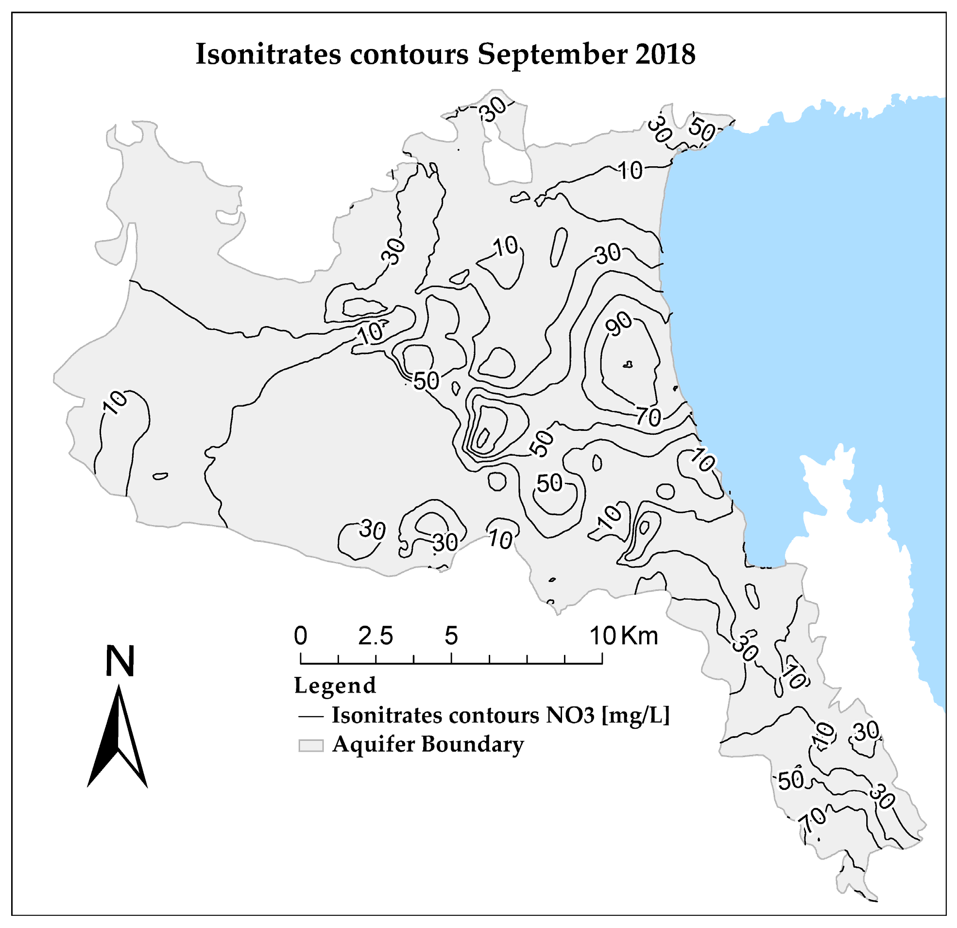
4.5. Nitrate Transport and Dispersion

The fluxes of nitrates concentration in the Almyros aquifer were simulated in a monthly transient mode for the stress period of October 1991 until September 2018. The transient advection and dispersion of nitrates that flow with the groundwater were simulated with the MT3DMS model. The model was run in the Almyros aquifer for the stress periods from October 1991 until September 2018.

The MT3DMS model was calibrated from October 1992 to September 2004 and validated from October 2013 to September 2015. The calibration procedure was performed with trial-and-error for the specification of the starting concentrations and several hydrogelogical zones of longitudinal dispersivity. The range of the longitudinal dispersivity values is 0.07–30 m with a spatial average of 3.5 m. The calibration results for the MT3DMS model indicate that the Nash–Sutcliffe model efficiency, the Pearson correlation, and the Index of Agreement are, on average, 0.81, 0.91, and 0.95, respectively. Summary statistics for the calibration and the validation period of the MT3DMS model are depicted in

Table 10. Summary efficiency statistics of the MT3DMS model.

MT3DMS	Calibration Average 1992–2004	Validation Average 2013–1015
Eff	0.80	0.82
R2	0.87	0.96
IA	0.95	0.95

.

Because of the intense hydraulic gradient of the western part of the aquifer, and even though the hydraulic conductivity is smaller than the coastal area, the nitrates are washed away with the groundwater towards the sea. The nitrate contamination that is observed in the aquifer is attributed to the agricultural fertilizers applied on the crops, and more specifically the spatial persistence of the pollution of the lower altitudes and hydraulic gradients follows inversely the magnitudes of the hydraulic conductivity zones.

The nitrates concentrations show a narrowing trend in the northern Lachanorema and Holorema sub-basin boundary in the winter of 2003, which is less discrete yet also evident in the rest of the aquifer. The central and central-coastal parts of the Almyros aquifer retain high nitrate concentrations for the simulation period 1991–2018. Nonetheless, the simulation results also indicate that the central Almyros aquifer has the potential to wash away the nitrate pollution, as it slowly does through the flow pathways, even in the hydrogeological clayish formations, but in the closed Xirorema sub-basin, the flow pattern of the region and the fertilizer applications impede the nitrates to fall more than 4 mg/L during the years 1991–2018.

Simulated isonitrate contours against the observed nitrate concentrations are presented for October 1992, September 2004, and March 2013 in Figure 17, Figure 18 and Figure 19. Additionally, scatterplots of the simulated nitrates concentrations of wells against their observed values indicate the validity of the results. The slopes and the intercepts of the regression lines of the nitrate concentrations scatterplots do not differ significantly from the line of perfect agreement (1:1 line) at α = 0.05 significance level using the two-sided t-test. The simulated nitrate pollution at the end of the simulation period in September 2018 is presented in Figure 20.

4.6. Chloride Solute Transport and Dispersion

The solute transport of chlorides in the Almyros aquifer was simulated the SEAWAT model in a monthly transient mode for the stress periods of October 1991 until September 2018. The model was run in the Almyros aquifer for the stress periods from October 1991 until September 2018, in the variable density mode, without taking under consideration viscosity and thermal effects. The parameter of longitudinal dispersivity (aL) was set previously in the MT3DMS model. The parameter of the effective molecular diffusion coefficient, which expresses the reactivity of the pollutant, for chlorides, as them being very conservative anions, was set at the value 10⁻¹⁰ [93]. The reference fluid density for the freshwater is 1000 kg/m³. The slope of density with the chloride concentration was estimated during the calibration/validation process of the model. The chloride concentration of the seawater for the Almyros coast, at the Constant-Head-Boundary that represents the sea, was set at 20,000 mg/L based on measurements of the study for the salinity of the Pagasitikos Gulf by [94].

The model was calibrated from October 1991 to September 2004 and validated for the period October 2005 to September 2007. The calibration procedure was performed with trial-and-error for the estimation of starting concentrations and of the slope of fluid density with the chloride concentrations. The slope of density with the chloride concentration was calibrated and validated at the value of 0.7143 × 10⁻⁶, for the simulation period considering the seawater intrusion with the variable density flow package of SEAWAT. The calibration results for the SEAWAT model indicate that the Nash–Sutcliffe model efficiency, the R-squared, and the Index of Agreement are, on average, 0.905, 0.945, and 0.980, respectively. Summary statistics for the calibration and the validation period of the SEAWAT model are shown in

Table 11. Statistical measures of the model’s efficiency for the calibration and validation periods.

SEAWAT	Calibration Average 1991–2004	Validation Average 2005–2007
Eff	0.92	0.89
R2	0.94	0.95
IA	0.98	0.98

.

The highest concentrations are generally observed in the northern part of the aquifer for the whole simulation period. Moreover, salinization occurs in the Platanorema and Xirorema basins in the south, especially because of the low altitude and the presence of lime formations close to the boundaries of the sub-basins. The seawater intrusion that is observed in the aquifer is attributed to the groundwater abstractions to address the crop water needs, the low altitude, the variability of the hydraulic conductivity of the coastal area, and the proximity to the sea. The seawater intrusion is exacerbated during the simulation years 1991–2018 on the northern coastline. Moreover, the groundwater in the northern sub-basins degraded from freshwater to brackish water, with an accelerating pace evident in 2001–2002, 2005–2006, and 2007–2008, while the rest of the simulation showed an accelerated trend but relatively stable variations of the chlorides’ concentrations trend. The coastal zone, at the proximities of 150 m and 300 m from the shore, in Kazani and Lachanorema sub-basins, is characterized by seawater of more than 12,300 mg/L and 4000 mg/L, respectively, at the end of 2018. Simulated isochlorides contours against observed chloride concentrations are presented for July 1992, and April 2007 in Figure 21 and Figure 22. Additionally, scatterplots of the simulated chloride concentrations against observed chloride concentrations indicate the validity of the simulation. The slopes and the intercepts of the regression lines of the chloride concentrations scatterplots do not differ significantly from the line of perfect agreement (1:1 line) at α = 0.05 significance level using the two-sided t-test.

The simulated chloride concentrations at the end of the simulation period in September 2018 in the north coastline surpass the upper pan-European limit of 12,300 mg/L. The simulated seawater intrusion in September 2018 is presented in Figure 23.

5. Discussion

Complex problems of the quantity and quality of water resources of coastal agricultural watersheds, and especially of the groundwater regarding the water table depletion, the nitrate contamination, and the seawater intrusion, are encountered in the semi-arid Mediterranean coastal region [1,2,3,4,5,6,7,8,9,10,11,12,13,14,15,16,17,18,23,28,29,32,39]. The developed integrated modeling system consisting of coupled and interrelated models of surface and groundwater hydrology, crop growth/nitrate leaching, and groundwater contaminant transport and its application in the Almyros basin, emphasize the significance of the integrated modeling for the study and the effective and accurate analysis of the spatiotemporal patterns of groundwater flow, nitrate pollution originated by fertilizer practices, and seawater intrusion [32]. The calibrated results of the Integrated Modeling System validate the effective implementation of the developed crop growth/nitrate leaching model (REPIC) for the simulation of crop yields and nitrate leaching in grid and basin/watershed scale. The R-ArcGIS based EPIC model (REPIC), along with the data handling tools and the optimization procedures, establish an advanced intrinsic connection with the surface hydrology model (UTHBAL) and the contaminant transport/aquifer pollution model (MT3DMS).

The application of the integrated modeling system in the Almyros basin proves that the modeling system is able to reproduce, in a holistic way [18,19,20,32], the observed water quantity and quality variables of the groundwater resources in the study area. Notably, in all t-tests [81], the slope and the intercept do not differ significantly from the hypothetical line of absolute agreement (at α = 0.05 significance level). The scores of all statistical measures of modeling efficiency are characterized by an excellent fit of the simulation parameters against the observed measurements [78,79,80] and validate the calibrated parameter values of the hydrological and the crop variables.

Hence, it is safe to estimate the water fluxes through the years of the simulation, taking into account the impacts of the variable density flow due to seawater intrusion on the aquifer balance [43]. The calculation of the water balance accounts for the recharge due to precipitation and irrigation return flows, the water abstractions due to agricultural and urban demands, and the seawater fluxes along the coastline boundary. The Almyros aquifer is recharged with 18.8 hm³/yr on average, while the water abstractions reach up to 29.7 hm³/yr resulting in a drop-down of the groundwater table and seawater intrusion of 0.3 hm³/yr but with adverse effects on the groundwater quality. The average water balance of the aquifer is presented in Figure 24. The water deficit is, on average, 12.02 hm³/yr. The aquifer’s annual water balance and the cumulative water deficit for the simulation period are presented in Figure 25. The water quantity pumped out of the aquifer is much larger than the quantity that is naturally replenished into the aquifer through the recharge and the irrigation return flows. Even though there are three years of positive water balance, the time-series of the aquifer’s water balance show an increasing trend of water deficit.

6. Conclusions

An Integrated Modeling System has been developed and presented for the evaluation of the quantity and quality of water resources, mainly of the groundwater resources, in coastal agricultural watersheds to address the need for integrated approaches in the simulation of water resources at appropriate spatiotemporal scales. The modeling system consists of coupled models of surface hydrology (UTHBAL), groundwater hydrology (MODFLOW), crop growth/nitrates leaching (REPIC), contaminant transport/nitrate pollution (MT3DMS), and seawater intrusion/aquifer salinization (SEAWAT). The modeling system holistically estimates and reproduces the monthly water balance and the groundwater pollution by nitrates and chlorides in coastal watersheds and aquifers in grid and watershed/basin scale. The accuracy of the simulated groundwater flow, nitrate pollution, and seawater intrusion are evaluated and validated with statistical measures of modeling efficiency in the coastal agricultural Almyros basin.

The results indicate that the causes of the negative water balance and drop-down of the water table are the limited use of surface water, the groundwater abstractions for agricultural use, and the cultivation of water demanding crops. Groundwater nitrate pollution is attributed to nitrate leaching due to the fertilizer applications for maximizing crop production, the geological formations with low hydraulic conductivity that withhold the washing the nitrates out of the Almyros basin aquifer, and the morphology and water flow regime of the aquifer. The seawater intrusion observed in the Almyros aquifer is caused by the increased crop water demands during the dry season and the intensive irrigation, and the granular and sandy geological character of the Almyros aquifer, especially near the shoreline.

Overall, the results of the application of the Integrated Modeling System prove that the modeling system is capable of simulating effectively complex water resources with increased accuracy. The modeling system may be used to simulate and evaluate various water resources management scenarios and strategies to overcome the water quantity and quality problems of coastal agricultural watersheds and the impacts of climate change on surface water and groundwater resources. The developed Integrated Modeling System may help to develop sustainable water resources management and agricultural practices.

References

1. Loukas, A.; Mylopoulos, N.; Vasiliades, L. A Modeling System for the Evaluation of Water Resources Management Strategies in Thessaly, Greece. Water Resour. Manag. 2007, 21, 1673–1702. [Google Scholar] [CrossRef]
2. Daskalaki, P.; Voudouris, K. Groundwater quality of porous aquifers in Greece: A synoptic review. Environ. Geol. 2008, 54, 505–513. [Google Scholar] [CrossRef]
3. Ghiglieri, G.; Barbieri, G.; Vernier, A.; Carletti, A.; Demurtas, N.; Pinna, R.; Pittalis, D. Potential risks of nitrate pollution in aquifers from agricultural practices in the Nurra region, northwestern Sardinia, Italy. J. Hydrol. 2009, 379, 339–350. [Google Scholar] [CrossRef]
4. Colombani, N.; Mastrocicco, M.; Prommer, H.; Sbarbati, C.; Petitta, M. Fate of arsenic, phosphate and ammonium plumes in a coastal aquifer affected by saltwater intrusion. J. Contam. Hydrol. 2015, 179, 116–131. [Google Scholar] [CrossRef] [PubMed]
5. Potot, C.; Féraud, G.; Schärer, U.; Barats, A.; Durrieu, G.; Le Poupon, C.; Travi, Y.; Simler, R. Groundwater and river baseline quality using major, trace elements, organic carbon and Sr–Pb–O isotopes in a Mediterranean catchment: The case of the Lower Var Valley (south-eastern France). J. Hydrol. 2012, 472–473, 126–147. [Google Scholar] [CrossRef]
6. Pulido-Velazquez, M.; Peña-Haro, S.; García-Prats, A.; Mocholi-Almudever, A.F.; Henriquez-Dole, L.; Macian-Sorribes, H.; Lopez-Nicolas, A. Integrated assessment of the impact of climate and land use changes on groundwater quantity and quality in the Mancha Oriental system (Spain). Hydrol. Earth Syst. Sci. 2015, 19, 1677–1693. [Google Scholar] [CrossRef] [Green Version]
7. Giménez-Forcada, E. Use of the Hydrochemical Facies Diagram (HFE-D) for the evaluation of salinization by seawater intrusion in the coastal Oropesa Plain: Comparative analysis with the coastal Vinaroz Plain, Spain. HydroResearch 2019, 76–84. [Google Scholar] [CrossRef]
8. Rosário Cameira, M.D.; Rolim, J.; Valente, F.; Mesquita, M.; Dragosits, U.; Cordovil, C.M. Translating the agricultural N surplus hazard into groundwater pollution risk: Implications for effectiveness of mitigation measures in nitrate vulnerable zones. Agric. Ecosyst. Environ. 2021. [Google Scholar] [CrossRef]
9. Telahigue, F.; Mejri, H.; Mansouri, B.; Souid, F.; Agoubi, B.; Chahlaoui, A.; Kharroubi, A. Assessing seawater intrusion in arid and semi-arid Mediterranean coastal aquifers using geochemical approaches. Phys. Chem. Earthparts A/B/C 2020, 115, 102811. [Google Scholar] [CrossRef]
10. Mohammad, A.H.; Jung, H.C.; Odeh, T.; Bhuiyan, C.; Hussein, H. Understanding the impact of droughts in the Yarmouk Basin, Jordan: Monitoring droughts through meteorological and hydrological drought indices. Arab. J. Geosci. 2018, 11, 103. [Google Scholar] [CrossRef] [Green Version]
11. Rachid, G.; Alameddine, I.; El-Fadel, M. SWOT risk analysis towards sustainable aquifer management along the Eastern Mediterranean. J. Environ. Manag. 2021, 279, 111760. [Google Scholar] [CrossRef] [PubMed]
12. Cobaner, M.; Yurtal, R.; Dogan, A.; Motz, L.H. Three dimensional simulation of seawater intrusion in coastal aquifers: A case study in the Goksu Deltaic Plain. J. Hydrol. 2012, 464–465, 262–280. [Google Scholar] [CrossRef]
13. EASAC. Groundwater in the Southern Member States of the European Union: An Assessment of Current Knowledge and Future Prospects; Country Report for Greece; European Academies Science Advisory Council: Harley, Germany, 2010; pp. 18–19. Available online: https://easac.eu/ (accessed on 21 January 2021).
14. European Commission. Verification of Vulnerable Zones Identified Under the Nitrate Directive, Greece; European Commission: Luxembourg, 2003; Available online: https://ec.europa.eu/ (accessed on 21 January 2021).
15. NCESD. Greece, State of the Environment Report, Summary; National Center of Environment and Sustainable Development: Athens, Greece, 2018; pp. 70–71. ISBN 978-960-99033-3-2. [Google Scholar]
16. Sidiropoulos, P.; Tziatzios, G.; Vasiliades, L.; Papaioannou, G.; Mylopoulos, N.; Loukas, A. Modelling flow and nitrate transport in an over-exploited aquifer of rural basin using an integrated system: The case of Lake Karla watershed. Proceedings 2018, 2, 667. [Google Scholar] [CrossRef] [Green Version]
17. EU. Report from the Commission: In Accordance with Article 3.7 of the Groundwater Directive 2006/118/EC on the Establishment of Groundwater Threshold Values; European Commission: Brussels, Belgium, 2010. [Google Scholar]
18. Madani, K.; Mariño, M.A. System dynamics analysis for managing Iran’s Zayandeh-Rud river basin. Water Resour. Manag. 2009, 23, 2163–2187. [Google Scholar] [CrossRef]
19. Mirchi, A. System Dynamics Modeling as a Quantitative-Qualitative Framework for Sustainable Water Resources Management: Insights for Water Quality Policy in the Great Lakes Region. Master’s Thesis, Michigan Technological University, Horton, MI, USA, 2013. [Google Scholar] [CrossRef]
20. Zomorodian, M.; Lai, S.H.; Homayounfar, M.; Ibrahim, S.; Fatemi, S.E.; El-Shafie, A.J.J.o.e.m. The state-of-the-art system dynamics application in integrated water resources modeling. J. Environ. Manag. 2018, 227, 294–304. [Google Scholar] [CrossRef]
21. Medici, G.; Baják, P.; West, L.J.; Chapman, P.J.; Banwart, S.A. DOC and nitrate fluxes from farmland; impact on a dolostone aquifer KCZ. J. Hydrol. 2020, 125658. [Google Scholar] [CrossRef]
22. Barthel, R.; Banzhaf, S. Groundwater and Surface Water Interaction at the Regional-scale—A Review with Focus on Regional Integrated Models. Water Resour. Manag. 2016, 30, 1–32. [Google Scholar] [CrossRef] [Green Version]
23. Milano, M.; Ruelland, D.; Fernandez, S.; Dezetter, A.; Fabre, J.; Servat, E.; Fritsch, J.-M.; Ardoin-Bardin, S.; Thivet, G. Current state of Mediterranean water resources and future trends under climatic and anthropogenic changes. Hydrol. Sci. J. 2013, 58, 498–518. [Google Scholar] [CrossRef]
24. Feng, D.; Zheng, Y.; Mao, Y.; Zhang, A.; Wu, B.; Li, J.; Tian, Y.; Wu, X. An integrated hydrological modeling approach for detection and attribution of climatic and human impacts on coastal water resources. J. Hydrol. 2018, 557, 305–320. [Google Scholar] [CrossRef]
25. Riad, P.; Graefe, S.; Hussein, H.; Buerkert, A. Landscape transformation processes in two large and two small cities in Egypt and Jordan over the last five decades using remote sensing data. Landsc. Urban Plan. 2020, 197, 103766. [Google Scholar] [CrossRef]
26. Bobba, A.G. Ground Water-Surface Water Interface (GWSWI) Modeling: Recent Advances and Future Challenges. Water Resour. Manag. 2012, 26, 4105–4131. [Google Scholar] [CrossRef]
27. Mylopoulos, N.; Kolokytha, E.; Loukas, A.; Mylopoulos, Y. Agricultural and water resources development in Thessaly, Greece in the framework of new European Union policies. Int. J. River Basin Manag. 2009, 7, 73–89. [Google Scholar] [CrossRef]
28. Sidiropoulos, P.; Loukas, A.; Georgiadou, I. Response of a degraded coastal aquifer to water resources management. Eur. Water 2016, 55, 67–77. [Google Scholar]
29. Daliakopoulos, I.N.; Tsanis, I.K.; Koutroulis, A.; Kourgialas, N.N.; Varouchakis, A.E.; Karatzas, G.P.; Ritsema, C.J. The threat of soil salinity: A European scale review. Sci. Total Environ. 2016, 573, 727–739. [Google Scholar] [CrossRef] [PubMed]
30. Ketabchi, H.; Mahmoodzadeh, D.; Ataie-Ashtiani, B.; Simmons, C.T. Sea-level rise impacts on seawater intrusion in coastal aquifers: Review and integration. J. Hydrol. 2016, 535, 235–255. [Google Scholar] [CrossRef]
31. Barthel, R.; Reichenau, T.G.; Krimly, T.; Dabbert, S.; Schneider, K.; Mauser, W. Integrated Modeling of Global Change Impacts on Agriculture and Groundwater Resources. Water Resour. Manag. 2012, 26, 1929–1951. [Google Scholar] [CrossRef]
32. Le Page, M.; Fakir, Y.; Aouissi, J. Chapter 7—Modeling for integrated water resources management in the Mediterranean region. In Water Resources in the Mediterranean Region; Zribi, M., Brocca, L., Tramblay, Y., Molle, F., Eds.; Elsevier: Amsterdam, The Netherlands, 2020; pp. 157–190. [Google Scholar] [CrossRef]
33. Burek, P.; Satoh, Y.; Kahil, T.; Tang, T.; Greve, P.; Smilovic, M.; Guillaumot, L.; Zhao, F.; Wada, Y. Development of the Community Water Model (CWatM v1.04)—A high-resolution hydrological model for global and regional assessment of integrated water resources management. Geosci. Model Dev. 2020, 13, 3267–3298. [Google Scholar] [CrossRef]
34. Odeh, T.; Mohammad, A.H.; Hussein, H.; Ismail, M.; Almomani, T. Over-pumping of groundwater in Irbid governorate, northern Jordan: A conceptual model to analyze the effects of urbanization and agricultural activities on groundwater levels and salinity. Environ. Earth Sci. 2019, 78, 40. [Google Scholar] [CrossRef] [Green Version]
35. Medici, G.; West, L.J.; Chapman, P.J.; Banwart, S.A. Prediction of contaminant transport in fractured carbonate aquifer types: A case study of the Permian Magnesian Limestone Group (NE England, UK). Environ. Sci. Pollut. Res. 2019, 26, 24863–24884. [Google Scholar] [CrossRef] [Green Version]
36. Wang, K.; Davies, E.G.R.; Liu, J. Integrated water resources management and modeling: A case study of Bow river basin, Canada. J. Clean. Prod. 2019, 240, 118242. [Google Scholar] [CrossRef]
37. Rossetto, R.; De Filippis, G.; Borsi, I.; Foglia, L.; Cannata, M.; Criollo, R.; Vázquez-Suñé, E. Integrating free and open source tools and distributed modelling codes in GIS environment for data-based groundwater management. Environ. Model. Softw. 2018, 107, 210–230. [Google Scholar] [CrossRef]
38. Wang, L.; Stuart, M.E.; Lewis, M.A.; Ward, R.S.; Skirvin, D.; Naden, P.S.; Collins, A.L.; Ascott, M.J. The changing trend in nitrate concentrations in major aquifers due to historical nitrate loading from agricultural land across England and Wales from 1925 to 2150. Sci. Total Environ. 2016, 542, 694–705. [Google Scholar] [CrossRef] [PubMed] [Green Version]
39. Ragab, R.; Bromley, J.; D’Agostino, D.R.; Lamaddalena, N.; Luizzi, G.T.; Dörflinger, G.; Katsikides, S.; Montenegro, S.; Montenegro, A. Water Resources Management Under Possible Future Climate and Land Use Changes: The Application of the Integrated Hydrological Modelling System, IHMS. In Integrated Water Resources Management in the Mediterranean Region: Dialogue towards New Strategy; Choukr-Allah, R., Ragab, R., Rodriguez-Clemente, R., Eds.; Springer: Dordrecht, The Netherlands, 2012; pp. 69–90. [Google Scholar] [CrossRef]
40. Harbaugh, A.W.; McDonald, M.G. User’s Documentation for MODFLOW-2000, an Update to the U.S. Geological Survey Modular Finite-Difference Ground-Water Flow Model; United States Government Printing Office: Washington, DC, USA, 2000. [Google Scholar]
41. Williams, J.R. The EPIC Model. In Computer Models of Watershed Hydrology; Singh, V.P., Ed.; Water Resources Publisher: Highlands Ranch, CO, USA, 1995; pp. 909–1000. [Google Scholar]
42. Zheng, C.; Wang, P.P. MT3DMS: A Modular Three-Dimensional Multi-Species Transport Model for Simulation of Advection, Dispersion and Chemical Reactions of Contaminants in Groundwater Systems, Documentation and User’s Guide; Contract Report SERDP-99-1; U.S. Army Engineer Research and Development Center: Vicksburg, MS, USA, 1999. [Google Scholar]
43. Guo, W.; Langevin, C.D. User’s Guide to SEAWAT: A Computer Program for Simulation of Three-Dimensional Variable-Density Ground-Water Flow; Techniques of Water-Resources Investigation; U.S. Geological Survey: Reston, VA, USA, 2002.
44. Liu, J.; Williams, J.R.; Zehnder, A.J.B.; Yang, H. GEPIC—Modelling wheat yield and crop water productivity with high resolution on a global scale. Agric. Syst. 2007, 94, 478–493. [Google Scholar] [CrossRef]
45. Gardener, M. Beginning R: The Statistical Programming Language; John Wiley & Sons: Hoboken, NJ, USA, 2012. [Google Scholar]
46. Pobuda, M. Using the R-ArcGIS Bridge: The Arcgisbinding Package. Available online: https://r.esri.com/assets/arcgisbinding-vignette.html (accessed on 21 January 2021).
47. TexasA & Magriliferesearch. EPIC & APEX Models. Available online: https://epicapex.tamu.edu/ (accessed on 21 January 2021).
48. U.S. Soil Conservation Service. National Engineering Handbook, Section 4—Hydrology; United States Department of Agriculture: Washington, DC, USA, 1972.
49. Thiessen, A.H. Precipitation averages for large areas. Mon. Weather Rev. 1911, 39, 1082–1089. [Google Scholar] [CrossRef]
50. Fiedler, F.R. Simple, Practical Method for Determining Station Weights Using Thiessen Polygons and Isohyetal Maps. J. Hydrol. Eng. 2003, 8, 219–221. [Google Scholar] [CrossRef]
51. Şen, Z. Average areal precipitation by percentage weighted polygon method. J. Hydrol. Eng. 1998, 3, 69–72. [Google Scholar] [CrossRef]
52. Thornthwaite, C.W. An Approach toward a Rational Classification of Climate. Geogr. Rev. 1948, 38, 55–94. [Google Scholar] [CrossRef]
53. Sidiropoulos, P.; Tziatzios, G.; Vasiliades, L.; Mylopoulos, N.; Loukas, A. Groundwater Nitrate Contamination Integrated Modeling for Climate and Water Resources Scenarios: The Case of Lake Karla Over-Exploited Aquifer. Water 2019, 11, 1201. [Google Scholar] [CrossRef] [Green Version]
54. McDonald, M.G.; Harbaugh, A.W.; original authors of MODFLOW. The History of MODFLOW. Groundwater 2003, 41, 280–283. [Google Scholar] [CrossRef]
55. Tziatzios, G.; Sidiropoulos, P.; Vasiliades, L.; Mylopoulos, N.; Loukas, A. Simulation of Nitrate Contamination in Lake Karla Aquifer. In Proceedings of the 14th International Conference on Environmental Science and Technology (CEST2015), Rhodes, Greece, 3–5 September 2015; Available online: https://cest2015.gnest.org/papers/cest2015_00121_oral_paper.pdf (accessed on 21 January 2021).
56. Psilovikos, A.A. Optimization models in groundwater management, based on linear and mixed integer programming. An application to a Greek hydrogeological basin. Phys. Chem. Earth 1999, 24, 139–144. [Google Scholar] [CrossRef]
57. Siarkos, I.; Latinopoulos, P. Modeling seawater intrusion in overexploited aquifers in the absence of sufficient data: Application to the aquifer of Nea Moudania, northern Greece. Hydrogeol. J. 2016, 24, 2123–2141. [Google Scholar] [CrossRef]
58. Kopsiaftis, G.; Mantoglou, A.; Giannoulopoulos, P. Variable density coastal aquifer models with application to an aquifer on Thira Island. Desalination 2009, 237, 65–80. [Google Scholar] [CrossRef]
59. Kourakos, G.; Mantoglou, A. Pumping optimization of coastal aquifers based on evolutionary algorithms and surrogate modular neural network models. Adv. Water Resour. 2009, 32, 507–521. [Google Scholar] [CrossRef]
60. Kaleris, V.K.; Ziogas, A.I. Using electrical resistivity logs and short duration pumping tests to estimate hydraulic conductivity profiles. J. Hydrol. 2020, 590, 125–277. [Google Scholar] [CrossRef]
61. Kopsiaftis, G.; Tigkas, D.; Christelis, V.; Vangelis, H. Assessment of drought impacts on semi-arid coastal aquifers of the Mediterranean. J. Arid Environ. 2017, 137, 7–15. [Google Scholar] [CrossRef]
62. Kritsotakis, M.; Tsanis, I.K. An integrated approach for sustainable water resources management of Messara basin, Crete, Greece. Eur. Water 2009, 27, 15–30. [Google Scholar]
63. Williams, J.; Jones, C.; Dyke, P. The EPIC Model and its Application. In Proceedings of the ICRISAT-IBSNAT-SYSS S International Symposium on Minimum Data Sets for Agrotechnology Transfer, Patancheru, India, 21–26 March 1983; pp. 111–121. [Google Scholar]
64. Wang, X.; Williams, J.; Gassman, P.; Baffaut, C.; Izaurralde, R.; Jeong, J.; Kiniry, J.R. EPIC and APEX: Model use, calibration, and validation. Trans. ASABE 2012, 55, 1447–1462. [Google Scholar] [CrossRef]
65. Sharpley, A.N.; Williams, J.R. EPIC-Erosion/Productivity Impact Calculator. I: Model Documentation. II: User Manual; Agricultural Research Service: Washington, DC, USA, 1990.
66. Liu, W.; Yang, H.; Liu, J.; Azevedo, L.B.; Wang, X.; Xu, Z.; Abbaspour, K.C.; Schulin, R. Global assessment of nitrogen losses and trade-offs with yields from major crop cultivations. Sci. Total Environ. 2016, 572, 526–537. [Google Scholar] [CrossRef]
67. Yin, Y.; Zhang, X.; Yu, H.; Lin, D.; Wu, Y.; Wang, J.a. Mapping Drought Risk (Maize) of the World. In World Atlas of Natural Disaster Risk; Shi, P., Kasperson, R., Eds.; Springer: Berlin/Heidelberg, Germany, 2015; pp. 211–226. [Google Scholar] [CrossRef]
68. Zhang, X.; Lin, D.; Guo, H.; Wu, Y.; Wang, J.a. Mapping Drought Risk (Rice) of the World. In World Atlas of Natural Disaster Risk; Shi, P., Kasperson, R., Eds.; Springer: Berlin/Heidelberg, Germany, 2015; pp. 243–258. [Google Scholar] [CrossRef]
69. Liu, J.; Fritz, S.; van Wesenbeeck, C.F.A.; Fuchs, M.; You, L.; Obersteiner, M.; Yang, H. A spatially explicit assessment of current and future hotspots of hunger in Sub-Saharan Africa in the context of global change. Glob. Planet. Chang. 2008, 64, 222–235. [Google Scholar] [CrossRef]
70. Liu, J.; Wiberg, D.; Zehnder, A.J.; Yang, H.J.I.S. Modeling the role of irrigation in winter wheat yield, crop water productivity, and production in China. Irrig. Sci. 2007, 26, 21–33. [Google Scholar] [CrossRef] [Green Version]
71. Koch, J.; Wimmer, F.; Schaldach, R.; Onigkeit, J. An integrated land-use system model for the Jordan River region. In Environmental Land Use Planning; Seth Appiah-Opoku InTechOpen: Tuscaloosa, AL, USA, 2012; Available online: https://www.intechopen.com/books/environmental-land-use-planning/an-integrated-land-use-system-model-for-the-jordan-river-region (accessed on 21 January 2021).
72. Zheng, C.; Bennett, G. Applied Contaminant Transport Modeling, 2nd ed.; Wiley-Interscience: New York, NY, USA, 2002; Volume 34. [Google Scholar]
73. Anderson, M.P.; Cherry, J.A. Using models to simulate the movement of contaminants through groundwater flow systems. Crit. Rev. Environ. Control 1979, 9, 97–156. [Google Scholar] [CrossRef]
74. Neuman, S.P. Universal scaling of hydraulic conductivities and dispersivities in geologic media. Water Resour. Res. 1990, 26, 1749–1758. [Google Scholar] [CrossRef]
75. Psaropoulou, E.T.; Karatzas, G.P. Pollution of nitrates—contaminant transport in heterogeneous porous media: A case study of the coastal aquifer of Corinth, Greece. Glob. Nest J. 2014, 16, 9–23. [Google Scholar] [CrossRef] [Green Version]
76. Guo, W.; Bennett, G.D. Simulation of Saline/Fresh Water Flows Using MODFLOW. In Proceedings of the MODFLOW 98 Conference, Golden, CO, USA, 4–8 October 1998; pp. 267–274. [Google Scholar]
77. Siarkos, I.; Latinopoulos, D.; Mallios, Z.; Latinopoulos, P. A methodological framework to assess the environmental and economic effects of injection barriers against seawater intrusion. J. Environ. Manag. 2017, 193, 532–540. [Google Scholar] [CrossRef]
78. Nash, J.E.; Sutcliffe, J.V. River flow forecasting through conceptual models part I—A discussion of principles. J. Hydrol. 1970, 10, 282–290. [Google Scholar] [CrossRef]
79. Colin Cameron, A.; Windmeijer, F.A.G. An R-squared measure of goodness of fit for some common nonlinear regression models. J. Econom. 1997, 77, 329–342. [Google Scholar] [CrossRef]
80. Matthews, J.; Bendig, A.W. The index of agreement: A possible criterion for measuring the outcome of group discussion. Speech Monogr. 1955, 22, 39–42. [Google Scholar] [CrossRef]
81. Smalheiser, N.R. Chapter 9—Null Hypothesis Statistical Testing and the t-test. In Data Literacy; Smalheiser, N.R., Ed.; Academic Press: New York, NY, USA, 2017; pp. 127–136. [Google Scholar] [CrossRef]
82. Lyra, A.; Pliakas, F.; Skias, S.; Gkiougkis, I. Implementation of DPSIR framework in the management of the Almyros basin, Magnesia Prefecture. Bull. Geol. Soc. Greece 2016, 50, 825–834. [Google Scholar] [CrossRef] [Green Version]
83. Stevenson, D.S. Irrigation Efficiency in Orchards. Can. Water Resour. J. 1980, 5, 102–110. [Google Scholar] [CrossRef]
84. Dewandel, B.; Gandolfi, J.-M.; de Condappa, D.; Ahmed, S. An efficient methodology for estimating irrigation return flow coefficients of irrigated crops at watershed and seasonal scale. Hydrol. Process. 2008, 22, 1700–1712. [Google Scholar] [CrossRef]
85. Willis, T.M.; Black, A.S.; Meyer, W.S. Estimates of deep percolation beneath cotton in the Macquarie Valley. Irrig. Sci. 1997, 17, 141–150. [Google Scholar] [CrossRef]
86. Panagos, P.; Van Liedekerke, M.; Jones, A.; Montanarella, L. European Soil Data Centre: Response to European policy support and public data requirements. Land Use Policy 2012, 29, 329–338. [Google Scholar] [CrossRef]
87. ESDAC. European Soil Data Centre, Joint Research Centre, European Commission. Available online: esdac.jrc.ec.europa.eu (accessed on 21 January 2021).
88. Soil Science Division Staff. Soil Survey Manual; Ditzler, C., Scheffe, K., Monger, H.C., Eds.; USDA Handbook, 18; Government Printing Office: Washington, DC, USA, 2017. Available online: https://www.nrcs.usda.gov/wps/portal/nrcs/detail/soils/scientists/?cid=nrcs142p2_054262 (accessed on 21 January 2021).
89. MEE. Ministry of Environment and Energy, Secretariat of National Environment and Water. Available online: http://lmt.ypeka.gr/public_view.html (accessed on 21 January 2021).
90. Merwade, V. Creating SCS Curve Number Grid Using HEC-GeoHMS. 2012. Available online: http://web.ics.purdue.edu/~vmerwade/tutorial.html (accessed on 21 January 2021).
91. Dastane, N. Effective Rainfall, FAO Irrigation and Drainage Paper No. 25; Food and Agriculture Organization: Rome, Italy, 1974. [Google Scholar]
92. Wichmann, W. World Fertilizer Use Manual; International Fertilizer Industry Association (IFA): Paris, France, 1992. [Google Scholar]
93. Tang, A.; Sandall, O.C. Diffusion coefficient of chlorine in water at 25–60 °C. J. Chem. Eng. Data 1985, 30, 189–191. [Google Scholar] [CrossRef]
94. Petihakis, G.; Triantafyllou, G.; Pollani, A.; Koliou, A.; Theodorou, A. Field data analysis and application of a complex water column biogeochemical model in different areas of a semi-enclosed basin: Towards the development of an ecosystem management tool. Mar. Environ. Res. 2005, 59, 493–518. [Google Scholar] [CrossRef] [PubMed]
Figure 1. Flow Chart of the Integrated Modeling System.
Water 13 00268 g001
Figure 2. Almyros aquifer system, elevation and streams of sub-basins, and locations of weather stations.
Water 13 00268 g002
Figure 3. (a) Geological Top View and (b) Section A-A’ (vertical) and Section B-B’ (horizontal), of the permeable formations of the Almyros aquifer system.
Water 13 00268 g003
Figure 4. (a) Locations of water table observation wells and (b) locations of groundwater abstraction wells.
Water 13 00268 g004
Figure 5. (a) Locations of nitrates observation wells and (b) locations of chlorides observation wells.
Water 13 00268 g005
Figure 6. Spatial distribution of (a) mean annual precipitation and (b) mean annual temperature for the years of 1961–2018.
Water 13 00268 g006
Figure 7. Mean monthly areal precipitation at the mean elevation of the Almyros basin and the sub-basins.
Water 13 00268 g007
Figure 8. Mean monthly areal temperature at the mean elevation of the Almyros basin and the sub-basins.
Water 13 00268 g008
Figure 9. (a) The water level of equal potential for July 1992 and (b) scatterplot of simulated against observed water table values.
Water 13 00268 g009
Figure 10. (a) The water level of equal potential for May 2006 and (b) scatterplot of simulated against observed water table values.
Water 13 00268 g010
Figure 11. (a) The water level of equal potential for June 2015 and (b) scatterplot of simulated against observed water table values.
Water 13 00268 g011
Figure 12. The water level of equal potential at the end of groundwater simulation in September 2018.
Water 13 00268 g012
Figure 13. (a) Average simulated crop yield per crop type, and (b) spatially simulated crop yields against spatially observed crop yields for the calibration period 2007–2012.
Water 13 00268 g013
Figure 14. (a) Average simulated crop yield per crop type, and (b) spatially simulated crop yields against spatially observed crop yields for the validation period 2013–2018.
Water 13 00268 g014
Figure 15. Simulated cumulative nitrates leached into the aquifer for the year of 2010.
Water 13 00268 g015
Figure 16. Simulated cumulative nitrates leached into the aquifer for the year of 2018.
Water 13 00268 g016
Figure 17. (a) Isonitrates contours for October 1992 and (b) scatterplot of simulated against observed nitrates concentration values.
Water 13 00268 g017
Figure 18. (a) Isonitrates contours for September 2004 and (b) scatterplot of simulated against observed nitrates concentration values.
Water 13 00268 g018
Figure 19. (a) Isonitrates contours for March 2013 and (b) scatterplot of simulated against observed nitrates concentration values.
Water 13 00268 g019
Figure 20. Isonitrates contours at the end of the simulation of nitrate pollution in September 2018.
Water 13 00268 g020
Figure 21. (a) Isochlorides contours for July 1992 and (b) scatterplot of simulated against observed chloride concentration values.
Water 13 00268 g021
Figure 22. (a) Isochlorides contours for April 2007 and (b) scatterplot of simulated against observed chloride concentration values.
Water 13 00268 g022
Figure 23. Isochlorides contours at the end of the simulation of seawater intrusion in September 2018.
Water 13 00268 g023
Figure 24. Average monthly water balance of the Almyros basin aquifer for the simulation years 1991–2018.
Water 13 00268 g024
Figure 25. Annual water balance and cumulative water deficit for the simulation years 1991–2018.
Water 13 00268 g025