
An Assessment of Vertical Land Movement to Support Coastal Hazards Planning in Washington State
by
 , ,
, ,
Tyler J. Newton
1,* ,
,
Ray Weldon
1,
Ian M. Miller
2,
David Schmidt
3,
Guillaume Mauger
4,
Harriet Morgan
4 and
Eric Grossman
5 1
Department of Earth Sciences, University of Oregon, Eugene, OR 97405, USA
2
Washington Sea Grant, Port Angeles, WA 98362, USA
3
Department of Earth and Space Sciences, University of Washington, Seattle, WA 98195, USA
4
Climate Impacts Group, Seattle, WA 98195, USA
5
US Geological Survey, Bellingham, WA 98225, USA
*
Author to whom correspondence should be addressed.
Water 2021, 13(3), 281; https://doi.org/10.3390/w13030281
Submission received: 1 December 2020
/
Revised: 19 January 2021
/
Accepted: 21 January 2021
/
Published: 24 January 2021
(This article belongs to the Special Issue Coastal Hazards Management)
Abstract
:The sea and land change elevation spatially and temporally from a multitude of processes, so it is necessary to constrain the movement of both to evaluate how coastlines will evolve and how those evolving coastlines will impact the natural and built environment over time. We combine land movement observations from global navigation satellite systems (GNSSs), leveling of geodetic monuments, and tide gauge records with a tectonic model of the Cascadia subduction zone to constrain absolute rates of vertical land movement in coastal Washington. We infer rates of vertical land movement in areas lacking direct observations by interpolating high-quality land movement observations and a discretely sampled interseismic locking model. Here we present a model of absolute vertical land movement that is combined with sea level rise estimates to inform local relative sea level projections on a community-scale. The most rapid vertical uplift (~3.5 mm/year) of the land is found across the northwest Olympic Peninsula, which currently outpaces sea level rise. Conversely, some areas, including a stretch of the northern Pacific Ocean coast from La Push to Kalaloch and the southern Puget Sound, are found to be subsiding at 0.5–1.0 mm/year, exacerbating the rate of relative sea level rise and thereby increasing the vulnerability of coastal communities.
1. Introduction
Coastlines support diverse ecosystems and a myriad of anthropogenic interests like communities, historical sites, and infrastructure. The safety and prosperity of coastal communities and the natural and built environment depend on our ability to plan for, predict, and adapt to changing conditions like rising mean sea level. Mean sea level change over time-frames of decades to centuries is primarily driven by thermal expansion of the ocean and mass loss from glaciers and ice sheets [1], but it can be modified locally by the vertical velocity of the land along the coast, leading to relative sea level change. Therefore, it is necessary to pair estimates of absolute sea level change with vertical land movement estimates in order to constrain relative sea level change and better assess the vulnerability of coastal resources. Vertical land movement (VLM) refers to the average long-term displacement of land surface in a geocentric reference frame that results from reorganization of the materials comprising Earth’s crust or from isostatic adjustment of the crust in response to a changing load [2]. Both anthropogenic processes (e.g., groundwater and hydrocarbon extraction, loading from water reservoirs, and anthropogenic compaction) and local natural processes (e.g., sediment compaction, tectonic deformation, and glacial isostatic adjustment) can cause vertical land movement at a variety of temporal (days to centuries) and spatial scales (millimeters to thousands of kilometers) [3,4]. Estimates of VLM are used to constrain models of these causal processes and assessments of earthquake, tsunami, and storm hazards [5,6]. The focus of this study is to constrain rates of land motion and relative sea level change to inform coastal hazards planning utilizing a method that is adaptable to other regions.
In coastal Washington state, on the Pacific coast of central North America, variable rates of coastal vertical land movement have been estimated by a variety of researchers, ranging between 4 mm/year uplift and −1 mm/year subsidence (Table S1). Regional patterns of VLM in coastal Washington are largely attributed to tectonic processes [7,8] from the Cascadia subduction zone (CSZ) to the west, and glacio-isostatic adjustment from deglaciation [9,10]. The CSZ hosts great earthquakes on a 500–530 year average recurrence interval [11] and is the predominant geodynamic process in this region generating crustal strain accumulation, in addition to clockwise forearc rotation [12]. Washington also hosts smaller crustal faults like the Seattle fault [13], as well as a multitude of volcanoes along the Cascadia volcanic arc. The geology of the coastal region is dominated by young oceanic basalt and sedimentary rock spanning the study area [14,15]. The area of interest in this study spans from the Pacific Ocean to the Cascadia volcanic arc, specifically along the coastline of Washington state.
Previous investigators have attempted to estimate rates of vertical land movement in the Pacific Northwest of the USA generally, and specifically in Washington state, motivated either by the desire to incorporate those movements into sea level assessments, or to inform seismic hazard assessments [16,17,18,19]. Most investigations have utilized one of three different methods for measuring long-term rates of vertical land movement:
(1) Leveling, which utilizes repeat measurements of geodetic monuments to derive a relative estimate of vertical land movement (i.e., vertical movement of one survey benchmark relative to another; see Burgette et al. [7]. Many early studies of vertical land movement referenced these relative rates to a geodetic reference frame by linking leveling results to estimates of vertical land movement derived from tide gauges.
(2) “Water-level differencing” methods, which difference water levels measured at tide gauges located close to each other to derive an estimate of vertical land movement at one tide gauge site relative to another. Many early studies of vertical land movement converted the relative rates derived using this approach to absolute rates using an assumed global average rate of sea level change (Table S1).
(3) Continuous global navigation satellite systems (CGNSS), which utilizes regularly-sampled measurements of position from fixed GNSS stations to derive an estimate of long-term vertical land movement rates in an absolute (i.e., geocentric) reference frame (i.e., movements relative to a center of mass of the Earth).
Mote et al. [20] conducted a review and discussion of investigations to characterize vertical land movement in Washington state. They compared three previous studies [21,22,23], all based primarily on leveling, to a preliminary CGNSS analysis. They found general agreement in regional patterns between these previous investigations, but discrepancies in the estimated rates of vertical land movement in some locations. More recent studies [16,17,20,24,25], summarized in Table S1, attempted to estimate rates and patterns of vertical land movement with the goal of resolving differences between relative sea level measured at tide gauges against vertical land movement rates at co-located CGNSS stations. These investigations provide a way to assess trends in regional absolute sea level, and compare the regional sea level trends against globally averaged rates. In general, these investigations rely on CGNSS datasets, typically from just one of several data providers, and also typically focus on a very limited number of locations in Washington state that are co-located with tide gauges. The most recent studies have also utilized GNSS glacial isostatic adjustment (GIA) corrections at tide gauges [18] and multiple CGNSS data providers [19].
In terms of resolving spatial variations in vertical land movement, most previous analyses suffered from either limited data, relying on estimates from just one data source or methodology, and/or a lack of estimates made directly on the coast. In addition, Snay et al. [16] point out discrepancies between different providers of continuous CGNSS-derived vertical land movement estimates (i.e., Table S1), which are also a consequence of the application of different methodologies, differing time-series lengths, or different analysis approaches. Finally, previous sea level rise assessments focused on Washington state [20,25] incorporated estimates of VLM into relative sea level projections, but without enough spatial resolution to resolve meaningful along-coast variations on a community scale. Partly as a consequence of these short-comings, local coastal managers in Washington state reported that they didn’t have adequate information to plan adequately for sea level rise [26]. Globally, studies have identified centimeter-scale VLM signals combining leveling and spaceborne SAR [27], however coastal Washington is heavily vegetated and regional mm/year scale VLM is outside of the observable range of standard SAR processing in our study region.
In this study, we present an approach to assimilate VLM estimates and their uncertainties, derived from multiple data types, in order to maximize the density of estimates on the coastal landscape and better account for the discrepancies between them. We also account for the primary VLM signal in areas without measurements by interpolating multiple data types and modeled vertical land velocities from interseismic tectonic locking on the CSZ, which dominates vertical velocities in instrumented areas. Our work reveals variable rates of vertical land movement in coastal Washington that may exacerbate or outpace sea level change depending on the location. We combine our model of vertical land movement with absolute sea level change projections and produce probabilistic relative sea level change projections, under two greenhouse gas scenarios and assuming no subduction zone earthquake, along the entirety of coastal Washington (first presented by Miller et al. [28]). The approach presented here is adaptable to any study area for which measurements and models of VLM exist, and represents an improvement over current methods of VLM estimation, resulting in dense and robust estimates of VLM that benefit coastal hazards planning.
2. Materials and Methods
2.1. Data
2.1.1. Continuous GPS
GNSS observations provide estimates of vertical land motion rates in a geocentric reference frame. While these estimates are relatively precise (with uncertainties on the order of several mm/year), solutions can vary depending on processing assumptions, such as regional filtering methods or how atmospheric water vapor is modeled. The observed differences in vertical rate estimates and their uncertainties across different CGNSS datasets [16] motivated us to develop an assimilative approach for deriving vertical land movement rates from CGNSS data from multiple GNSS datasets (Table S2). We based our best estimates and associated uncertainties for CGNSS sites on the distribution in estimated rates and uncertainties across datasets provided by five different providers: Nevada Geodetic Laboratory [29], NASA JPL [30], Scripps Orbit and Permanent Array Center [31], Pacific Northwest Geodetic Array Geodesy Laboratory [32], and UNAVCO [33]. All of the GNSS data are in the ITRF2008 reference frame.
Data were downloaded for all available stations in the Pacific Northwest (inclusive of western Oregon, western Washington and southern British Columbia) from the five different CGNSS data processing groups. To address the disparity in rates and uncertainties (Figure S1) across CGNSS-derived estimates we first classified CGNSS stations into high/low quality categories based on the length of the time-series over which vertical velocity solutions were estimated from a visual examination of the relationship between uncertainty and time-series length (Figure S1). Records exceeding nine years were initiallyclassified as “high-quality”. Records shorter than nine years were classified as “high-quality” only if at least three of the vertical rate estimates across the different processing groups agreed to within ±1 mm/year. Stations designated as “low-quality” via this filtering step were excluded from further analysis. This quality assessment procedure classified 117 out of 188 total CGNSS stations in our area of interest (Figure 1) as “high-quality”.
The best estimate of the vertical rate at a CGNSS site was designed to take into account differences in solutions between the five different datasets, and was arrived at through a multi-step process. First, an outlier detection algorithm was applied to the “high-quality” CGNSS sites with more than three estimates from different processing groups, in order to separate out stations with longer time-series but for which one of the processing group’s estimates was dramatically different from the others. For this assessment we applied a median absolute deviation approach to identify outliers, with an outlier cut-off value of 6. Therefore, any value with a median absolute deviation of more than 6 times the median value was eliminated from the calculation of a mean velocity across data processing centers.
Next, we calculated a weighted average of the individual vertical rate estimates, where the weighting was scaled by an adjusted uncertainty in the station vertical velocity:
where xi are the reported velocities from the different processing groups and σi are the adjustment uncertainties for each observation. The weighted averaging approach has the effect of making those vertical velocities with smaller adjusted uncertainties carry more weight in the vertical velocity averaging process. The magnitude of the uncertainty estimates for CGNSS-based vertical land movement observations were not consistent across data providers, with some providing a relatively narrow uncertainty range and others estimating a wide uncertainty range (Figure S1a, Table S2). However, the relative scale of the uncertainties was generally consistent within and across datasets and was assumed to be indicative of the relative scale of uncertainty of the estimates between stations. In order to utilize the weighted averaging approach described in Equation (1) the different uncertainty estimates for each station needed to be adjusted. As a result, we developed an adjustment process to rescale uncertainties and facilitate comparisons across datasets. We assume that the uncertainty in the vertical rate estimate should asymptote to a stable value as more observations become available (i.e., due to a longer observational record). We therefore corrected the uncertainty estimates by: (1) Calculating the mean uncertainty for each of the five CGNSS data sets for all high-quality stations. (2) Estimating a scaling factor for the reported uncertainties for each processing center such that the mean uncertainty for all high-quality stations is consistent between processing centers. This ensures that the variability in uncertainty is preserved between stations. (3) Multiplying all CGNSS vertical uncertainties by the appropriate scaling factor assigned to each processing center (Table S2). To estimate the uncertainty of our final, average vertical velocity rates for each station we calculated the standard deviation of the vertical rate estimates for a station, as calculated by the different processing groups (Figure 1). This approach was more conservative than propagating the error associated with each rate.
2.1.2. Tide Gauges
Water-level differencing, in our case differencing monthly-averaged water levels from tide gauges, provides an estimate of the relative difference in vertical land velocity rates between tide gauges. There are two approaches: “single-differencing”, which assumes that the stations are close enough to each other that they experience the same variations in sea level; and “double-differencing”, which does not assume that the stations share an absolute sea-level trend, but rather attempts to directly estimate the absolute sea level pattern at a tide gauge using altimetry [34]. We conducted a single-differencing analysis that employed the following steps: (1) Obtain monthly average water level data from the Permanent Service for Mean Sea Level for a set of 23 stations in Oregon, Washington and British Columbia. (2) Choose a set of “reference stations” (Table S3) that were co-located with a “high quality” CGNSS station (within 5km, though 3 of the 4 reference stations were located less than 500 m apart), and included a long (>20 years) water level record. (3) Difference each station’s monthly sea level against those from each of the four reference stations. (4) Remove the mean seasonal signal in the resulting differenced time-series, by subtracting out the long-term average for each calendar month. (5) Estimate the trend and standard error in the linear regression, accounting for auto-correlation (using the variance inflation factor approach described in Zervas [35]. (6) Adjust the estimated relative vertical velocity to an absolute rate by adding it to the best estimate vertical rate derived from the high quality CGNSS station co-located with each “reference” water level station. The uncertainties assigned to the rates derived using this approach (Figure 2) were estimated by propagating the uncertainty assigned to the co-located CGNSS station.
2.1.3. Leveling
Leveling is a surveying method that is used to measure the relative height difference between two nearby benchmarks. By repeating a survey of the benchmarks at a later time and differencing against an earlier data set, it is possible to measure the rate of change in the elevation difference between benchmarks. This method provides relative changes in height between adjacent stations (i.e., tilt) and must be tied to a nearby CGNSS or tide gauge station in order to be placed in a reference frame. We incorporate vertical rates from leveling in our analysis using the methodologies and data described in Burgette et al. [7], Krogstad et al. [36], Mitchell et al. [22], and Schmidt et al. [37], which utilize historical leveling data dating to the 1920′s (Figure 3), by adjusting earlier tide gauge-based reference frames to ours, based on CGNSS as described above. We also added two new lines from Westport and Tacoma east. These relative rates were converted to absolute rates of vertical land movement by attaching leveling lines to nearby high-quality CGNSS stations. Relative vertical rates for a series of benchmarks along a leveling line (typically located along transportation corridors) were adjusted to best fit the vertical land movement estimates of one or more nearby CGNSS stations or tide gauges. The uncertainty of the CGNSS station is assigned to the nearest leveling point, then uncertainty is propagated from that point using the measurement uncertainties of successive leveling observations. We also recalculated the uncertainties for the north-south line on the east side of the Olympic Peninsula that were too small in previous work that we incorporated.
2.2. Tectonic Model
Within our study area we found a total of 519 VLM rate estimates from CGNSS, leveling, and tide gauges (Figure 4). However, there are large stretches of our study area for which vertical land movement observations do not exist (Figure 4). The limited data that exist near the coast and the spatially-dense leveling lines (roughly perpendicular to the CSZ) suggest large gradients in vertical land movement over short distances, which could lead to a misrepresentation of rates of vertical land movement on the shoreline in areas where most observations are collected farther inland. Specifically, at locations on the north and central coast near La Push and Kalaloch, Washington, observations point to subsidence on the shoreline, and rapid uplift only a short distance inland. Further, an interpolation of the combined vertical land velocity observations yields unphysical edge effects since all data were acquired on land and there are no seafloor observations to constrain the western edge of the interpolation. To first order, the large-scale pattern of deformation revealed by vertical land movement observations in our area of interest can be explained by interseismic locking of the megathrust on the Cascadia subduction zone, and large gradients in near-coast deformation are likely [38].
We incorporated a discretely sampled velocity field derived from a forward model of a locked fault slipping at depth in the Cascadia subduction zone in our analysis to place geophysical constraints on the expected vertical signal in regions without direct measurements. The interseismic locking model uses the modeling framework of Burgette et al. [7], which was solely focused on modeling leveling data in Oregon, but expanded to Washington state and constrained by both vertical leveling and horizontal GPS velocities by Schmidt et al. [37]. This locking model was compared to and combined with other similar locking models to constrain seismic hazards in the Pacific Northwest for the United States National Seismic Hazard Maps [5] in Frankel and Petersen [8]. The interseismic locking model assumes that the slip deficit rate is equal to the plate convergence rate (i.e., fully locked) near the trench and decreases exponentially in the transition zone. The locking model is also assumed to vary smoothly along strike. The depth of the lower edge of the fully locked zone and lower edge of the transition zone as a function of latitude are optimized through a grid search. The resulting locking model is largely similar to other locking models for Cascadia [5], where fault locking is primarily confined to the megathrust at depths shallower than 20 km (coinciding with sections of the megathrust west of the coastline). In using the locking model for this paper, we use the distribution of the slip-rate deficit on the megathrust to forward predict uplift rate across our focus area. To better match the new refined data set, we have applied a uniform vertical shift to account for our different reference frame.
The locking model is intended to physically model the crustal strain associated with the convergence of the Juan de Fuca and North American plates, which is the dominant signal in the geodetic data. This strain is elastically stored in the crust and will eventually be released in a future megathrust earthquake on the subduction zone, thus our estimates of vertical land velocity are not valid after the next megathrust earthquake. Our tectonic model does not model other processes, like compaction of sediments, erosion, or the movement of shallow crustal faults that may result in the vertical movement of the ground. Vertical rate estimates were extracted from the locking model at a grid spacing of 0.2 degree (16–22 km). These were combined with our other vertical rate estimates for the purposes of interpolating a best-estimate vertical velocity field. The modeled vertical rates were arbitrarily assigned a relatively large uncertainty of ± 2 mm/year to minimize the influence of the model in areas with ample observations. The locking model is not used to replace or modify the observations, but rather is used to more accurately interpolate vertical velocity estimates at locations between the observations, particularly where large gradients exist.
2.3. Interpolation
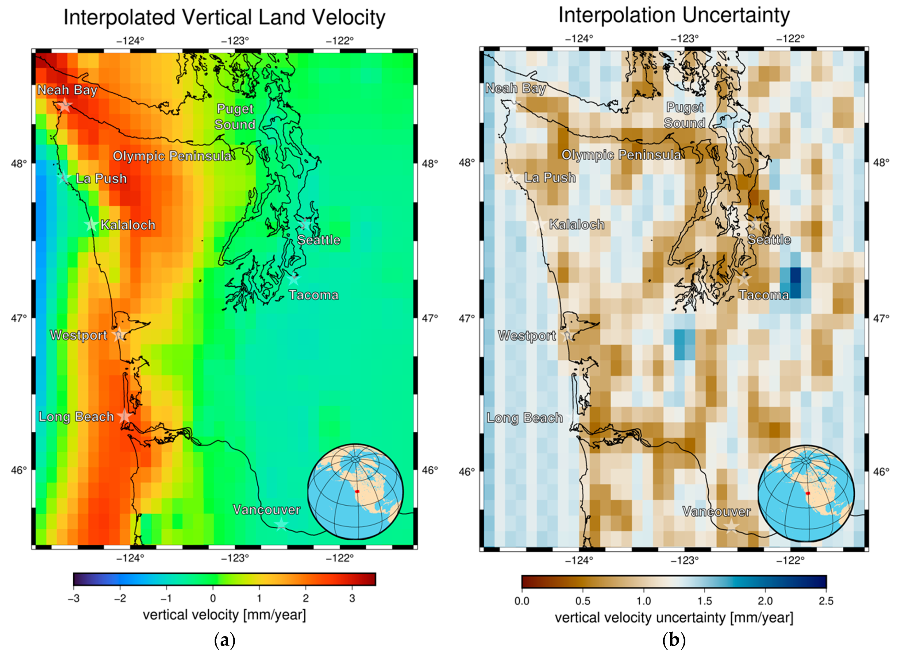
We interpolate between all discrete observations and gridded tectonic model velocity field points to represent the vertical land velocity as a surface that is a function of the longitude and latitude, or a height field with z = f(longitude, latitude). Since we model the vertical velocity as a height field, the field may not contain vertical slopes or overhangs, neither of which are realistic representations of land movement at the scale of interest (~10 km). We first generate a scattered interpolant from the combined observed and modeled vertical velocities using Delaunay triangulation with bivariate linear interpolation [39]. Triangulation of the scattered vertical velocities in the longitude-latitude plane generates a continuous surface composed of triangular pieces joined at edges, or a triangulated irregular network, over the area of interest. The triangulated irregular network represents a piecewise interpolation scheme in which bivariate linear interpolation is applied to each triangle. We then query the interpolant at a grid spacing of 0.1 degree to yield an interpolated vertical land velocity height field (Figure 5a; Data S3).
To include a measure of uncertainty for interpolated vertical velocities we employ bootstrapping. At each location with observed or modeled vertical velocities we specify a normal distribution defined by the vertical velocity as the distribution mean and the standard deviation. We then randomly sample each distribution and generate an interpolated vertical velocity height field, repeating the process 10,000 times. The reported interpolation uncertainty is the standard deviation, with N-1 normalization, of the 10,000 interpolation iterations at each grid point, thus representing the variation in interpolated vertical velocity given hypothetical variations in the data. In essence, the uncertainty presented in Figure 5b is a measure of the stability of the interpolation results.
3. Results
We model the vertical velocity field of coastal Washington as an interpolated height field to produce the most spatially comprehensive estimate of vertical land motion for coastal Washington to date. Previous investigators (Table S1) have found variations in coastal vertical land movement ranging from ~1.0 mm/year of subsidence (in central Puget Sound) to approximately 3–4 mm/year of uplift (on the northwest tip of the Olympic Peninsula). Overall, we find the same general patterns suggested by previous investigators, and resolve many of the finer-scale variations between tide stations and leveling lines. In addition, we find the most rapid rates of coastal uplift associated with the northwest tip of the Olympic Peninsula (Figure 5). Our results also suggest:
- A strong west-to-east gradient in rates of vertical land movement across our area of interest that is particularly pronounced along a transect following the Strait of Juan de Fuca (Figure 5a), and that we attribute to subduction zone processes.
- Low rates of subsidence (<1 mm/year) in Puget Sound, but with a south-to-north gradient showing higher rates of subsidence to the south and lower rates to the north, consistent with the pattern expected for glacio-isostatic adjustment.
- Rapid uplift along the southwest Washington coast, but with a large uncertainty in estimated rates, including Westport and the Long Beach Peninsula.
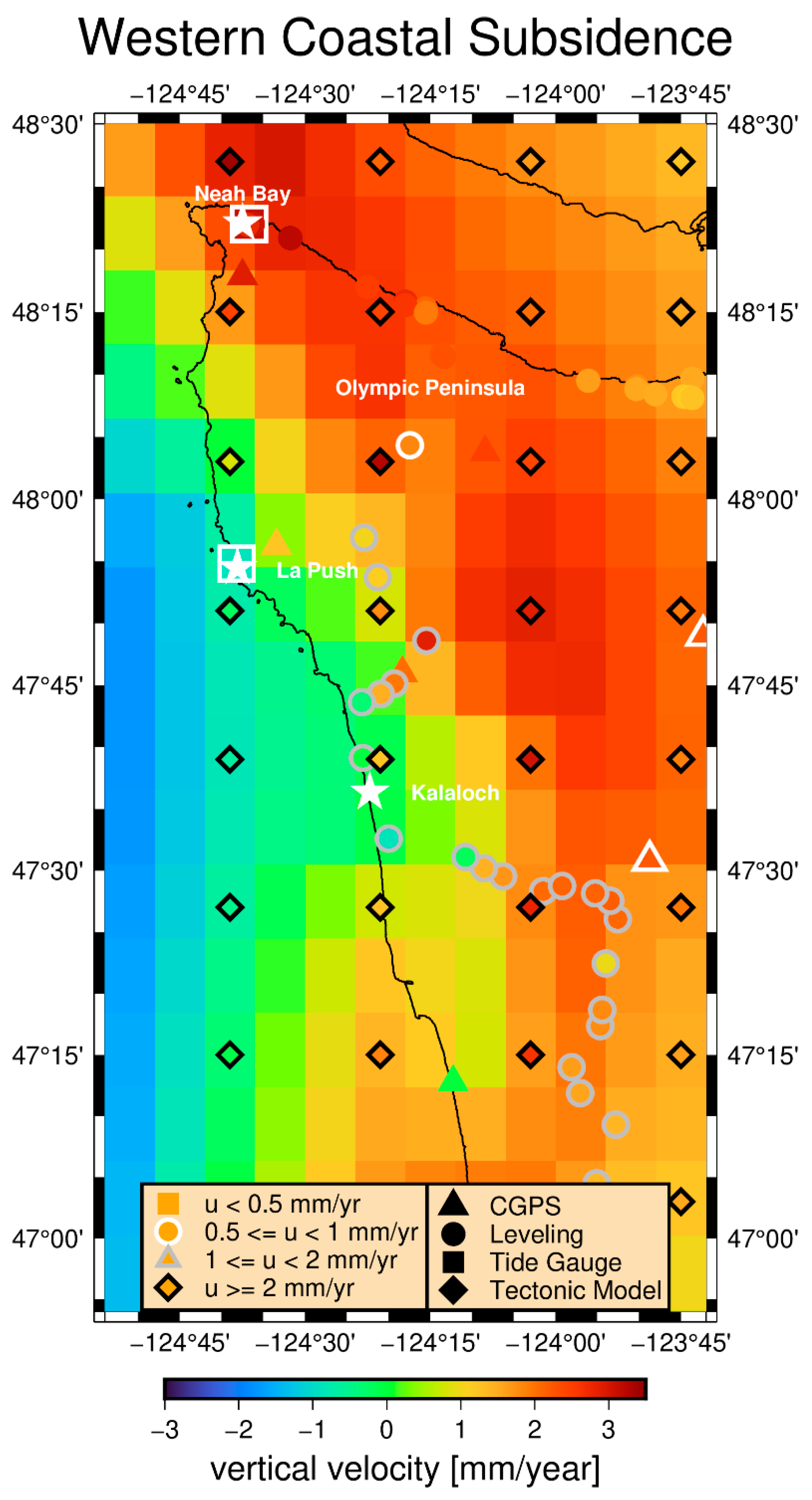
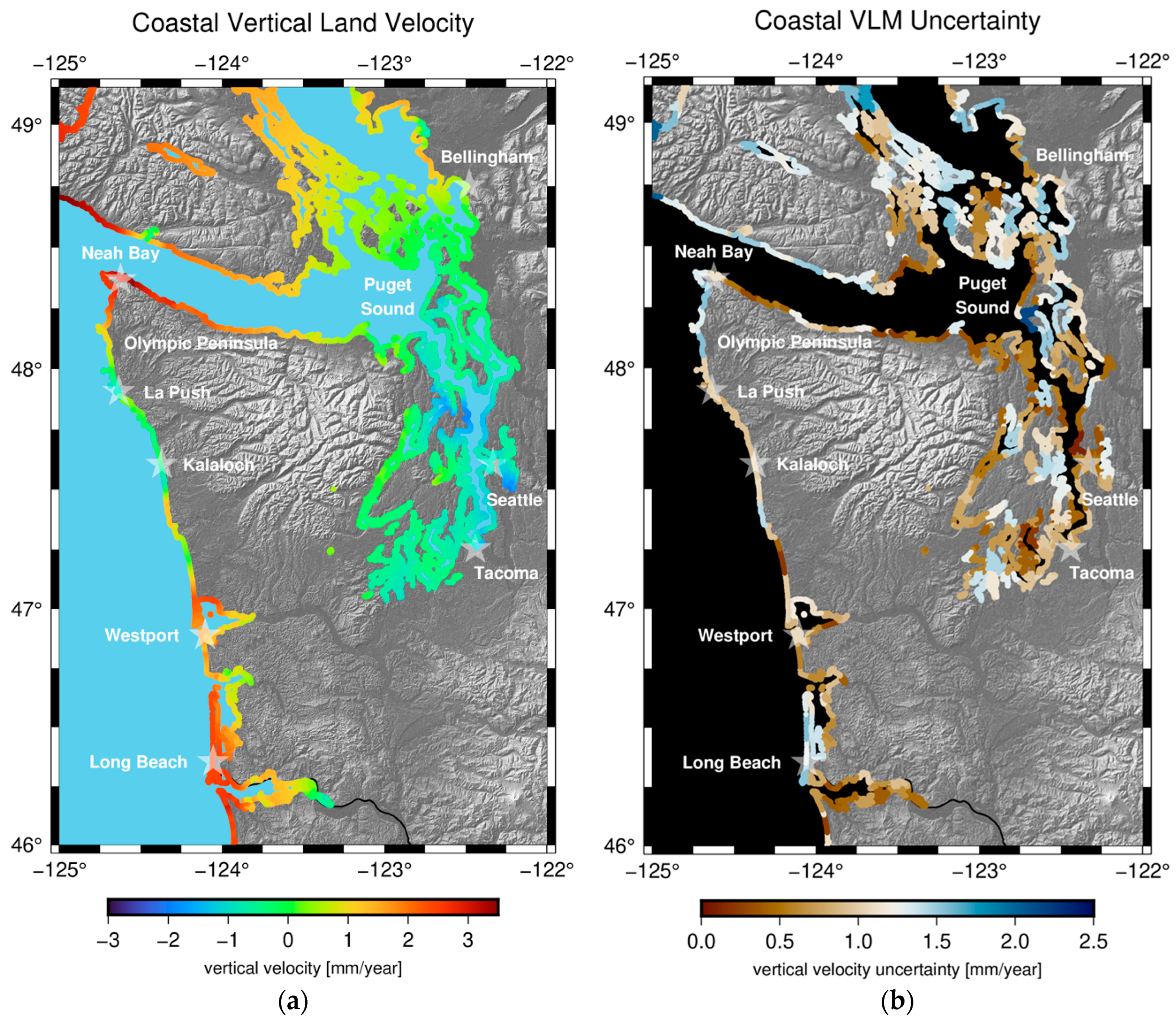
We also find a broad area of coastal subsidence along the northern Pacific Ocean coast of Washington state (Figure 6). Previous studies generally do not make spatially continuous VLM estimates throughout this area, though some studies did find evidence of subsidence in the same area [23,34]. Other studies estimated uplift (e.g., [14]) along this section of coast, or observations in this area were not considered (e.g., [11]). Figure 6 shows the northwest region of study area where we find subsidence along coastal Washington, indicated by the colored grid that constitutes the interpolated vertical velocity surface, in addition to VLM observations and the gridded tectonic model that inform the interpolation. Observations of VLM from leveling, tide gauges, and CGNSS stations in this region show spatial vertical velocity gradients (0.2 mm/km) that are steeper than those present in the tectonic locking model (0.1 mm/km; Figure 6). Figure 7a shows the interpolant queried at a sub-kilometer scale along the coastline to depict smooth variations in coastal VLM, and Figure 7b shows the associated uncertainty.
Despite the density of observations utilized in this assessment, areas of large uncertainty remain, either due to uncertainties in the observations themselves (Figure S2), large gradients in the rate of vertical land movement, or a lack of observations in certain parts of the landscape. We quantify the uncertainty associated with our interpolated model of vertical land motion (Figure 5b). It is important to note, there are also areas of uplift or subsidence driven by processes other than interseismic strain accumulation and at scales smaller than the resolution of this study are not well-represented in our model or uncertainty analysis. Areas containing VLM observations with high uncertainties (observations with black outlines in Figure 4) correspond to the areas in our model with the highest uncertainty (dark blue colors in Figure 5b). The focus of this study is to provide robust estimates of vertical land movement along the coast, so our estimated rates of VLM in inland Washington, particularly near volcanoes and the eastern boundary of our model, do not fully characterize contemporary crustal movements considering interseismic strain accumulation decreases with distance from the subduction zone.
4. Discussion
Our estimates of VLM and the associated uncertainties, when combined with sea level projections, provide insights about current and future relative sea level changes for coastal communities throughout Washington that can supply local coastal managers with the information necessary to plan adequately for sea level rise (Figure 7a,b). An assumption of this study, supported by over 70 years of tide gauge and repeated leveling observations, is that the observed and modeled rates of vertical land movement are constant over the interseismic period, so we discuss the implications of a Cascadia subduction zone earthquake on vertical land motion in the region. Additionally, we further explore spatial patterns in the resulting interpolated vertical velocity field and identify a convolved north-south vertical velocity gradient, likely from glacial isostatic adjustment, that will continue whether there is a Cascadia earthquake or not. To conclude this study, we explore the effect of the assumed GIA signal on an elastic dislocation model of Cascadia subduction zone locking, and thus could impact earthquake hazard level estimates.
4.1. Relative Sea Level Change
We combine our estimate of interpolated vertical land movement with absolute sea level change projections to produce probabilistic relative sea level change projections for 171 locations throughout coastal Washington under two greenhouse gas scenarios, first presented by Miller et al. [28]. We utilize a single absolute sea level rise projection for all of Washington state, as the regional variations in absolute sea level change are not well resolved over this scale [28]. The low and high greenhouse gas scenarios (RCP 4.5 and 8.5 [40]) reflect different emissions trajectories that depend on human behavior over decades; thus, we do not speculate which scenario is more likely. The projections presented in Figure 8 incorporate uncertainties from the models and observations incorporated into the assessment, which includes the range of expected mass loss from the Antarctica and Greenland ice sheets. Our projections are presented as the likelihood that sea level change will meet or exceed a particular offset from contemporary sea level, or the probability of exceedance. We utilize an approach for estimating absolute sea level change adapted from Kopp et al. [41] for seven Washington state tide gauges, fully described by Miller et al. [28].
Because interseismic strain accumulation from tectonic locking on the CSZ is the primary VLM signal in the coastal Pacific Northwest on a regional scale, relative sea level rise patterns mirror the opposite of the tectonic uplift signal. Areas like Neah Bay that experience rapid vertical uplift (Figure 7) will, in general, experience less relative sea level rise, and sea level drop is present in cases where vertical land velocities outpace rates of absolute sea level rise. Conversely, regions experiencing land subsidence, like Tacoma (Figure 7), will have rates of relative sea level rise that are greater than the rate of absolute sea level rise. The effect of large uncertainties in vertical land velocities can be seen in the projections for sites like Long Beach peninsula, resulting in a large difference between probability of exceedance projections. Relative sea level projections for 171 locations along the Washington coast are available and we refer readers to Miller et al. [28] for additional details of our relative sea level rise assessment.
4.2. Cascadia Earthquake Scenario
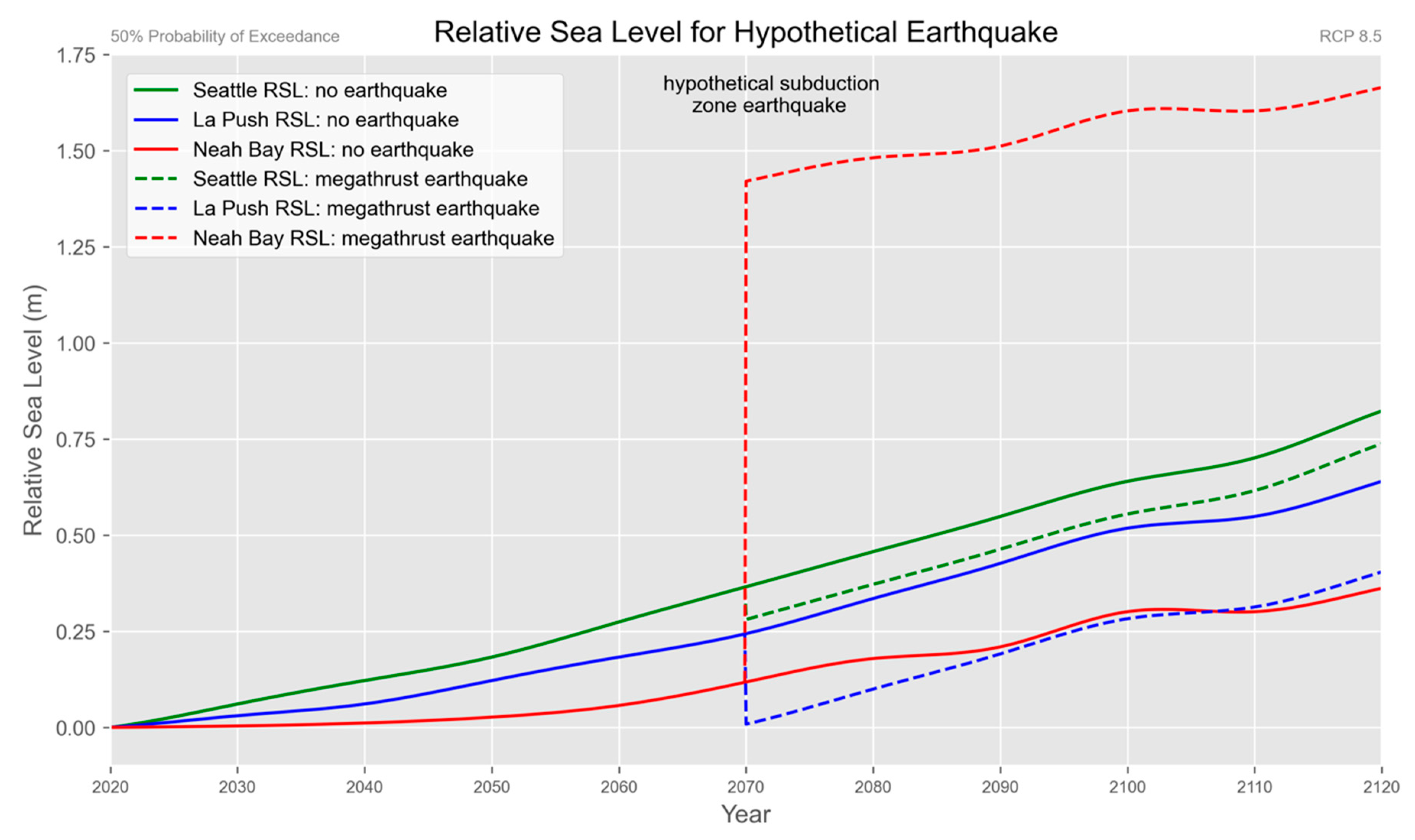
We assume constant rates of vertical land movement during an interseismic period, and thus constant strain accumulation. This assumption is reasonable given that: (1) we are late in the interseismic period when deformation rates are expected to be constant in time [38], and (2) nearly constant rates of VLM are observed for the ~70 year tide gauge and leveling record. However, the uplift proximal to the coast indicates that strain energy is accumulating in the crust and will be released in the next megathrust earthquake. A large earthquake would result in coseismic land displacements that void our assumption of a constant deformation rate and produce temporally and spatially variable rates of vertical land movement. Additionally, rapid and spatially variable post-seismic deformation follows large earthquakes, resulting from viscoelastic stress transfer that continues decades after the earthquake. The Tohoku earthquake that struck central Japan on March 11 2011, for example, resulted in coastal subsidence of more than 1 m in places along the east coast of Japan [42]. Localized uplift of the coast is also possible depending on the geometry of the subduction zone and proximity of the coast to the zone of locking. Figure 9 provides simplified examples of the effect of a megathrust earthquake on relative sea level for three sites from 2020 to 2120 with and without a hypothetical megathrust earthquake at the year 2070, assuming that our estimated VLM rate is entirely due to subduction processes and full recovery of the VLM rate summed over the hypothetical interseismic period (1700–2070). The true coseismic VLM depends on the type and timing of rupture (Table S4), but previous studies that focus on constraining the complexities of coseismic displacements report a range of coseismic subsidence consistent with our first-order estimate for areas experiencing uplift [6,43,44,45]. Despite the simplifications and assumptions inherent to the hypothetical coseismic land motions depicted in Figure 9, the region of subsidence we find from La Push to Kalaloch may produce coseismic uplift rather than the coseismic subsidence expected in regions experiencing interseismic uplift, depending on the complexities of subduction processes. Thus, Figure 9 serves to reiterate the importance of constraining VLM and the driving processes to inform hazard assessments.
4.3. North-South VLM Gradient
We find two dominant signals in the data that are most evident in our study area: an east-west gradient consistent with locking along the Cascadia subduction zone (CSZ), and a smaller magnitude south-north gradient that is most apparent east of the region affected by subduction zone locking (Figure S3a). The two gradients are superimposed in the coastal region, although VLM data are routinely used to inform subduction zone models that assume the data are absent of independent sources of motion. To isolate the north-south vertical velocity gradient, we utilize the gridding of our interpolated surface and find the mean value for all rows of 0.1 degree by 0.1 degree cells east of −123.0° longitude, then we subtract the mean for each row from all 0.1 degree by 0.1 degree cells in that row. The longitude-averaged north-south vertical velocity ranges from 0.6 mm/year in the north (49.0° latitude) to −0.7 mm/year in the south (45.5° latitude). This simple estimate of the observed north-south gradient assumes that the vertical velocity gradient is strictly north-south trending, but is intended to provide only a first-order approximation of the signal.
To assess the contribution of this vertical velocity gradient, we generate simple elastic dislocation models (as in Schmidt et al. [37]) for CSZ locking with and without the north-south gradient by subtracting the observed gradient east of the Puget Sound from all of Washington, including the CSZ locking-dominated gradient in coastal Washington, west of the Cascades. We compare the predicted horizontal strain from each model to the observed horizontal strain, measured from horizontal GNSS motion. Correcting for the north-south gradient in our model reduces the RMS error by 2% and better predicts the observed strain in Washington. Additionally, the correction extends the modeled extent of tectonic locking farther downdip near La Push (Figure S3b). Since the observed vertical and horizontal strain best fit our model with the north-south regional uplift gradient removed, we hypothesize that this gradient is superimposed on the coastal region, and likely unrelated to the CSZ. We speculate that the observed north-south gradient is GIA, consistent with previous studies [4,9]; however, other mechanisms are possible, including a 3D viscoelastic response to past CSZ rupture, rotation of the forearc, and local subsidence associated with the broader Puget Sound forearc basin region. Regardless of the source, the convolved signal implies that multiple overlapping processes are driving vertical land movement in Washington state.
5. Conclusions
We generate the most spatially comprehensive estimate of VLM to date for coastal Washington and find moderate rates of subsidence throughout the Puget Sound and near La Push, separated by a broad region of rapid uplift that extends south to Oregon. Combining VLM with forecast sea level rise provides relative sea level change for coastal Washington. A north-south vertical velocity gradient, consistent with GIA, is apparent in VLM observations, and correction of an elastic dislocation model for this signal yields lower errors in the predicted horizontal strain in Washington when compared to observations. The dominant VLM pattern in this region is consistent with interseismic strain accumulation on the CSZ.
Ideally, future research will combine new techniques and spatially-comprehensive data sets to produce dense and robust estimates of VLM. Previous VLM assessments predominantly infer uplift in the region spanning La Push to Kalaloch where we find subsidence [20,25]. Conflicting VLM results pose challenges for hazards planning in coastal communities; thus, future studies that further constrain vertical uplift rates in areas with few direct observations are critical to understanding VLM and its sources throughout Washington. Since relative sea level projections utilize annually compounding rates of VLM, misestimation of vertical rates may lead to large errors in projected relative sea level and misuse of community resources leading to potential ramifications for community vulnerability. Further, VLM estimates inform coseismic deformation models that are critical for accurate estimation of tsunami hazards, requiring robust, spatially-comprehensive, and repeatable VLM estimates.
Supplementary Materials
The following are available online at https://www.mdpi.com/2073-4441/13/3/281/s1, Figure S1: CGNSS Uncertainties and Corrected Uncertainties, Figure S2: Data, Tectonic Model, and Interpolated Land Velocity, Figure S3: N-S Vertical Velocity Gradient and Spatial Extent of Locking, Table S1: Review of VLM Estimates for Coastal Washington State, Table S2: CGPS Datasets Summary, Table S3: Water Level Differencing Reference Stations, Table S4: Coseismic Deformation Models, Data S1: Tectonic Locking Model Points, Data S2: VLM Observations, Data S3: Interpolated Vertical Velocity Grid, Data S4: Interpolation Uncertainty Grid, Data S5: Coastal VLM, Data S6: Coastal VLM Uncertainty.
Author Contributions
Conceptualization, I.M.M., T.J.N., R.W., D.S., G.M., and E.G.; methodology, I.M.M., R.W., T.J.N., D.S., G.M., and H.M.; data analysis and interpretation, T.J.N., R.W., I.M.M., D.S., G.M., and H.M.; writing, T.J.N., I.M.M., D.S., and R.W.; visualization, T.J.N., I.M.M., and D.S. All authors have read and agreed to the published version of the manuscript.
Funding
The project is primarily funded by a grant from the NOAA Regional Coastal Resilience Grants Program (grant #NA16NOS4730015). Additional funds were provided by the State of Washington as well as the Pacific Northwest Climate Impacts Research Consortium (CIRC), which is partially funded by the Regional Integrated Sciences and Assessments program under NOAA grant #NA15OAR4310145.
Institutional Review Board Statement
Not applicable.
Informed Consent Statement
Not applicable.
Data Availability Statement
The data presented in this study are available in the supplementary material.
Acknowledgments
We thank Mark Welch for his work on assimilating GNSS data sets, which was the starting point of our GNSS analysis. Figures in this manuscript were generated using PyGMT [46,47] and Matplotlib [48]. Any use of trade, firm, or product names is for descriptive purposes only and does not imply endorsement by the U.S. Government.
Conflicts of Interest
The authors declare no conflict of interest. The funders had no role in the design of the study; in the collection, analyses, or interpretation of data; in the writing of the manuscript, or in the decision to publish the results.
References
- Church, J.A.; White, N.J. Sea-Level Rise from the Late 19th to the Early 21st Century. Sol. Var. Clim. 2011. [CrossRef]
- Moucha, R.; Forte, A.M.; Mitrovica, J.X.; Rowley, D.B.; Quéré, S.; Simmons, N.A.; Grand, S.P. Dynamic topography and long-term sea-level variations: There is no such thing as a stable continental platform. Earth Planet. Sci. Lett. 2008, 271, 101–108. [Google Scholar] [CrossRef]
- Wöppelmann, G.; Marcos, M. Vertical land motion as a key to understanding sea level change and variability. Rev. Geophys. 2016, 54, 64–92. [Google Scholar] [CrossRef] [Green Version]
- Clark, J.; Mitrovica, J.X.; Latychev, K. Glacial isostatic adjustment in central Cascadia: Insights from three-dimensional Earth modeling. Geol. 2019, 47, 295–298. [Google Scholar] [CrossRef]
- Petersen, M.D.; Moschetti, M.P.; Powers, P.M.; Mueller, C.S.; Haller, K.M.; Frankel, A.D.; Zeng, Y.; Rezaeian, S.; Harmsen, S.C.; Boyd, O.S.; et al. Documentation for the 2014 update of the United States national seismic hazard maps. Open-File Report 2014. [Google Scholar] [CrossRef]
- Gao, D.; Wang, K.; Insua, T.L.; Sypus, M.; Riedel, M.; Sun, T. Defining megathrust tsunami source scenarios for northernmost Cascadia. Nat. Hazards 2018, 94, 445–469. [Google Scholar] [CrossRef]
- Burgette, R.J.; Weldon, R.J.; Schmidt, D.A. Interseismic uplift rates for western Oregon and along-strike variation in locking on the Cascadia subduction zone. J. Geophys. Res. Space Phys. 2009. [Google Scholar] [CrossRef] [Green Version]
- Frankel, A.; Petersen, M. Models of Earthquake Recurrence and Down-Dip Edge of Rupture for the Cascadia Subduction Zone; Appendix P of Uniform California Earthquake Rupture Forecast, Version 3 (UCERF3); US Geological Survey: Reston, VA, USA, 2012.
- Yousefi, M.; Milne, G.A.; Love, R.; Tarasov, L. Glacial isostatic adjustment along the Pacific coast of central North America. Quat. Sci. Rev. 2018, 193, 288–311. [Google Scholar] [CrossRef]
- James, T.S.; Gowan, E.J.; Wada, I.; Wang, K. Viscosity of the asthenosphere from glacial isostatic adjustment and subduction dynamics at the northern Cascadia subduction zone, British Columbia, Canada. J. Geophys. Res. Space Phys. 2009. [Google Scholar] [CrossRef]
- Goldfinger, C.; Nelson, C.H.; Morey, A.E.; Johnson, J.E.; Patton, J.R.; Karabanov, E.B.; Gutierrez-Pastor, J.; Eriksson, A.T.; Gracia, E.; Dunhill, G.; et al. Turbidite Event History—Methods and Implications for Holocene Paleoseismicity of the Cascadia Subduction Zone; Professional Paper; U.S. Geological Survey: Reston, VA, USA, 2012. [CrossRef]
- Wells, R.E.; McCaffrey, R. Steady rotation of the Cascade arc. Geology 2013, 41, 1027–1030. [Google Scholar] [CrossRef] [Green Version]
- Troost, K.G.; Booth, D.B. Geology of Seattle and the Seattle area, Washington. In Landslides and Engineering Geology of the Seattle, Washington, Area; The Geological Society of America: Boulder, CO, USA, 2008; Volume 20, pp. 1–36. [Google Scholar] [CrossRef] [Green Version]
- Schuster, J.E. Geologic Map of Washington State; Washington State Department of Natural Resources: Olympia, WA, USA, 2005.
- Miller, M.B.; Cowan, D.S. Roadside Geology of Washington; Mountain Press: Missoula, MT, USA, 2017. [Google Scholar]
- Snay, R.; Cline, M.; Dillinger, W.; Foote, R.; Hilla, S.; Kass, W.; Ray, J.; Rohde, J.; Sella, G.; Soler, T. Using global positioning system-derived crustal velocities to estimate rates of absolute sea level change from North American tide gauge records. J. Geophys. Res. Space Phys. 2007, 112. [Google Scholar] [CrossRef] [Green Version]
- Mazzotti, S.; Jones, C.; Thomson, R.E. Relative and absolute sea level rise in western Canada and northwestern United States from a combined tide gauge-GPS analysis. J. Geophys. Res. Space Phys. 2008, 113. [Google Scholar] [CrossRef] [Green Version]
- Hamlington, B.; Thompson, P.; Hammond, W.C.; Blewitt, G.; Ray, R.D. Assessing the impact of vertical land motion on twentieth century global mean sea level estimates. J. Geophys. Res. Oceans 2016, 121, 4980–4993. [Google Scholar] [CrossRef]
- MontilletiD, J.-P.; Melbourne, T.I.; Szeliga, W. GPS Vertical Land Motion Corrections to Sea-Level Rise Estimates in the Pacific Northwest. J. Geophys. Res. Oceans 2018, 123, 1196–1212. [Google Scholar] [CrossRef]
- Mote, P.; Petersen, A.; Reeder, S.; Shipman, H.; Whitely Binder, L. Sea level rise in the coastal waters of Washington State. 2008. Available online: https://digital.lib.washington.edu/researchworks/bitstream/handle/1773/34589/1.pdf?sequence=1 (accessed on 3 January 2018).
- Holdahl, S.R.; Faucher, F.; Dragert, H. Contemporary vertical crustal motion in the Pacific Northwest. Slow Deform. Transm. Stress Earth 1989, 49, 17–29. [Google Scholar]
- Mitchell, C.E.; Vincent, P.; Weldon, R.J.; Richards, M.A. Present-day vertical deformation of the Cascadia Margin, Pacific Northwest, United States. J. Geophys. Res. Space Phys. 1994, 99, 12257–12277. [Google Scholar] [CrossRef]
- Verdonck, D. Contemporary vertical crustal deformation in Cascadia. Tectonophysics 2006, 417, 221–230. [Google Scholar] [CrossRef]
- Wöppelmann, G.; Míguez, B.M.; Bouin, M.-N.; Altamimi, Z. Geocentric sea-level trend estimates from GPS analyses at relevant tide gauges world-wide. Glob. Planet. Chang. 2007, 57, 396–406. [Google Scholar] [CrossRef] [Green Version]
- National Research Council; Division on Earth and Life Studies; Ocean Studies Board; Board on Earth Sciences and Resources; Committee on Sea Level Rise in California. Oregon, and Washington. Sea-Level Rise for the Coasts of California, Oregon, and Washington: Past, Present, and Future; National Academies Press: Washington, DC, USA, 2012; Available online: https://play.google.com/store/books/details?id=_oBs2zAwtGgC (accessed on 15 January 2018).
- Halvorsen, E.; Mooney, J. Planning for change: Climate adaptation survey results, Washington State, USA, 2013; Report No.: WSG-TR 14-01; Washington Sea Grant: Seattle, WA, USA, 2014. [Google Scholar]
- Hung, W.-C.; Hwang, C.; Chen, Y.-A.; Zhang, L.; Chen, K.-H.; Wei, S.-H.; Huang, D.-R.; Lin, S.-H. Land Subsidence in Chiayi, Taiwan, from Compaction Well, Leveling and ALOS/PALSAR: Aquaculture-Induced Relative Sea Level Rise. Remote. Sens. 2017, 10, 40. [Google Scholar] [CrossRef] [Green Version]
- Miller, I.; Morgan, H.; Mauger, G.; Newton, T.; Weldon, R.; Schmidt, D.; Welch, M.; Grossman, E. Projected Sea Level Rise for Washington State—A 2018 Assessment; Washington Coastal Resilience Project; Washington Sea Grant: Seattle, WA, USA, 2018; Available online: https://cig.uw.edu/resources/special-reports/sea-level-rise-in-washington-state-a-2018-assessment/ (accessed on 5 November 2020).
- Blewitt, G.; Hammond, W.C. Harnessing the GPS Data Explosion for Interdisciplinary Science. Eos 2018, 99, 1–2. [Google Scholar] [CrossRef]
- Zumberge, J.F. Automated GPS Data Analysis Service. GPS Solutions 1999, 2, 76–78. [Google Scholar] [CrossRef]
- Jamason, P.; Bock, Y.; Fang, P.; Gilmore, B.; Malveaux, D.; Prawirodirdjo, L.; Scharber, M. SOPAC Web site (http://sopac.ucsd.edu). GPS Solutions 2004, 8, 272–277. [Google Scholar] [CrossRef]
- Miller, M.; Johnson, D.; Rubin, C.; Dragert, H.; Endo, E.; Humphreys, E. GPS Monitoring of the Cascadia Margin: The Pacific Northwest Geodetic Array (PANGA). Eos Trans AGU. 1997, 78, 46. [Google Scholar]
- Herring, T.A.; Melbourne, T.I.; Murray, M.H.; Floyd, M.; Szeliga, W.; King, R.W.; Phillips, D.A.; Puskas, C.; Santillan, M.; Wang, L. Plate Boundary Observatory and related networks: GPS data analysis methods and geodetic products. Rev. Geophys. 2016, 54, 759–808. [Google Scholar] [CrossRef]
- Santamaría-Gómez, A.; Gravelle, M.; Wöppelmann, G. Long-term vertical land motion from double-differenced tide gauge and satellite altimetry data. J. Geodesy 2013, 88, 207–222. [Google Scholar] [CrossRef]
- Zervas, C.E. Sea level variations of the United States, 1854–2006; Silver Spring: Silver Spring, MD, USA, 2009. Available online: https://repository.library.noaa.gov/view/noaa/2565 (accessed on 5 November 2020).
- Krogstad, R.D.; Schmidt, D.A.; Weldon, R.J.; Burgette, R.J. Constraints on accumulated strain near the ETS zone along Cascadia. Earth Planet. Sci. Lett. 2016, 439, 109–116. [Google Scholar] [CrossRef] [Green Version]
- Schmidt, D.; Weldon, R.; Burgette, R.; Krogstad, R. The distribution of interseismic locking on the Cascadia Subduction Zone constrained by leveling, tide gauge, and GPS data. AGUFM. G53C–05. 2011. Available online: https://earthquake.usgs.gov/static/lfs/nshm/workshops/PACNW2012/Schmidt2012CSZ.pdf (accessed on 5 November 2020).
- Wang, K.; Wells, R.; Mazzotti, S.; Hyndman, R.D.; Sagiya, T. A revised dislocation model of interseismic deformation of the Cascadia subduction zone. J. Geophys. Res. Space Phys. 2003, 108. [Google Scholar] [CrossRef] [Green Version]
- Amidror, I. Scattered data interpolation methods for electronic imaging systems: A survey. J. Electron. Imaging 2002, 11. [Google Scholar] [CrossRef]
- Van Vuuren, D.P.; Edmonds, J.; Kainuma, M.; Riahi, K.; Thomson, A.; Hibbard, K.; Hurtt, G.C.; Kram, T.; Krey, V.; Lamarque, J.-F.; et al. The representative concentration pathways: An overview. Clim. Chang. 2011, 109, 5–31. [Google Scholar] [CrossRef]
- E Kopp, R.; Horton, R.M.; Little, C.M.; Mitrovica, J.X.; Oppenheimer, M.; Rasmussen, D.J.; Strauss, B.H.; Tebaldi, C. Probabilistic 21st and 22nd century sea-level projections at a global network of tide-gauge sites. Earth’s Futur. 2014, 2, 383–406. [Google Scholar] [CrossRef]
- Imakiire, T.; Koarai, M. Wide-area land subsidence caused by “the 2011 Off the Pacific Coast of Tohoku Earthquake”. Soils Found. 2012, 52, 842–855. [Google Scholar] [CrossRef] [Green Version]
- Witter, R.C.; Zhang, Y.J.; Wang, K.; Priest, G.R.; Goldfinger, C.; Stimely, L.; English, J.T.; Ferro, P.A. Simulated tsunami inundation for a range of Cascadia megathrust earthquake scenarios at Bandon, Oregon, USA. Geosph. 2013, 9, 1783–1803. [Google Scholar] [CrossRef] [Green Version]
- Nelson, A.R.; Shennan, I.; Long, A.J. Identifying coseismic subsidence in tidal-wetland stratigraphic sequences at the Cascadia subduction zone of western North America. J. Geophys. Res. Space Phys. 1996, 101, 6115–6135. [Google Scholar] [CrossRef]
- Leonard, L.; Hyndman, R.D.; Mazzotti, S. Coseismic subsidence in the 1700 great Cascadia earthquake: Coastal estimates versus elastic dislocation models. GSA Bull. 2004, 116, 655. [Google Scholar] [CrossRef] [Green Version]
- Uieda, L.; Tian, D.; Leong, W.J.; Toney, L.; Newton, T.; Wessel, P. PyGMT: A Python interface for the Generic Mapping Tools. Zenodo. 2020. [Google Scholar] [CrossRef]
- Wessel, P.; Luis, J.; Uieda, L.; Scharroo, R.; Wobbe, F.; Smith, W.; Tian, D. The Generic Mapping Tools Version 6. Geochem. Geophys. Geosystems 2019, 20, 5556–5564. [Google Scholar] [CrossRef] [Green Version]
- Hunter, J.D. Matplotlib: A 2D Graphics Environment. Comput. Sci. Eng. 2007, 9, 90–95. [Google Scholar] [CrossRef]
Figure 1.
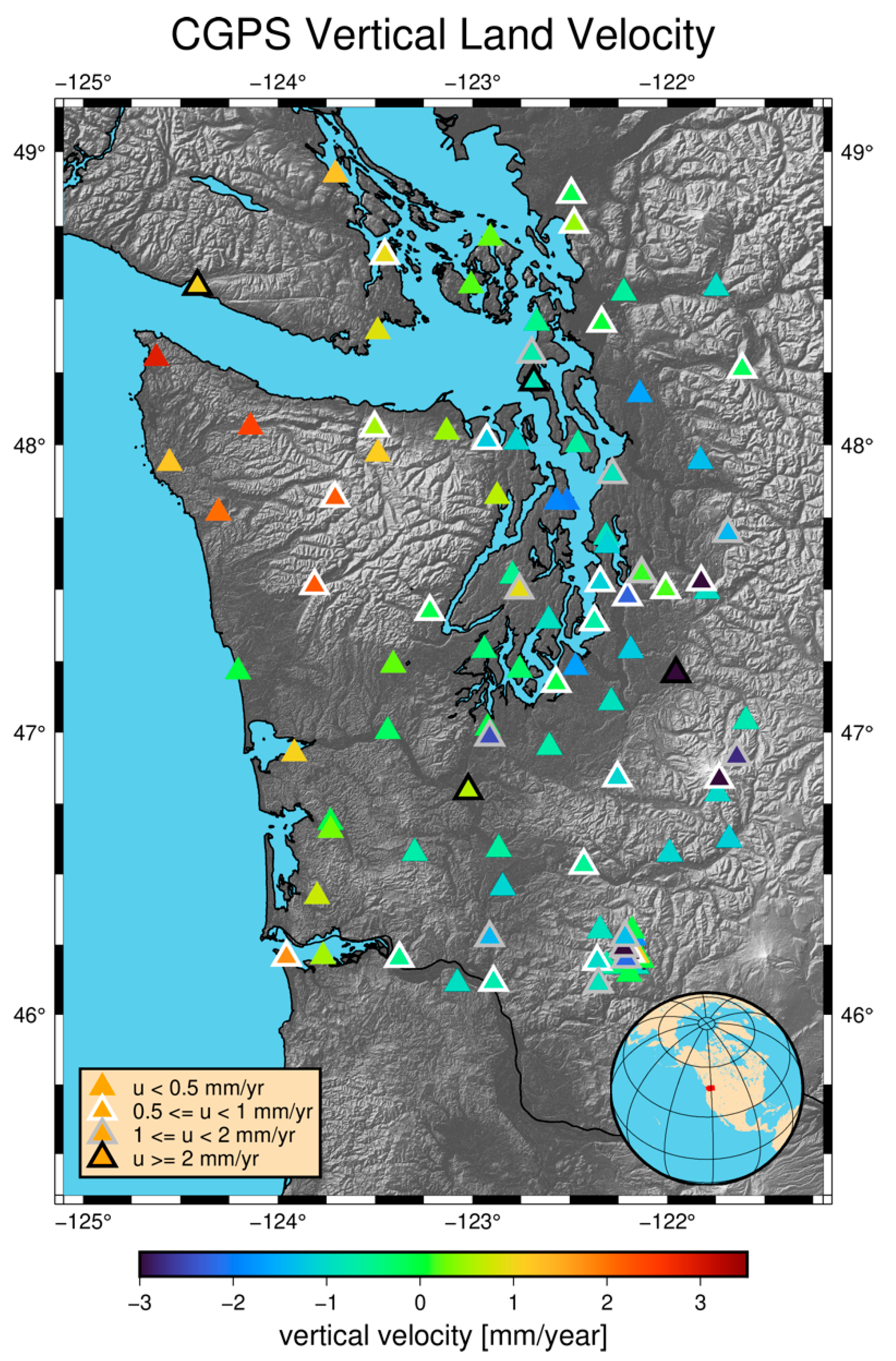
Continuous GNSS measurements of vertical land movement from five data providers. Vertical velocity is denoted by marker color and uncertainty is denoted by marker outline, expressed as millimeters per year (mm/yr). A transition from uplift, at the western tip of the Olympic Peninsula, to subsidence east is apparent in the CGNSS observations. Refer to Figure 2 for names of places. North is up.
Figure 1.
Continuous GNSS measurements of vertical land movement from five data providers. Vertical velocity is denoted by marker color and uncertainty is denoted by marker outline, expressed as millimeters per year (mm/yr). A transition from uplift, at the western tip of the Olympic Peninsula, to subsidence east is apparent in the CGNSS observations. Refer to Figure 2 for names of places. North is up.

Figure 2.
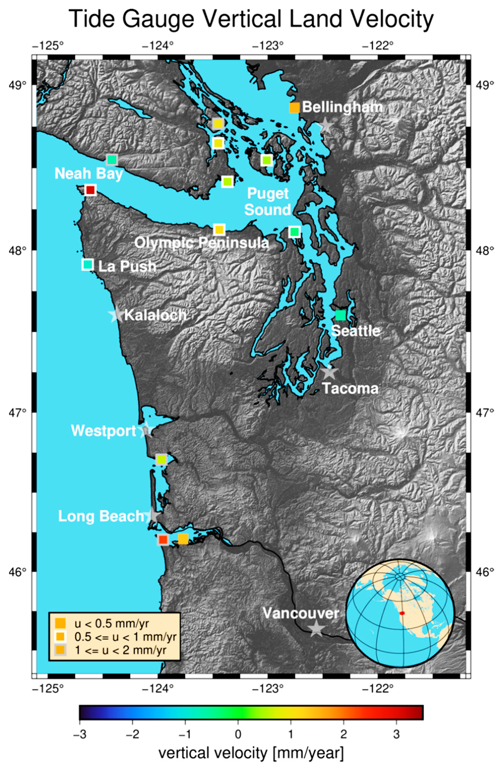
Measurements of vertical land movement derived from water level differencing of tide gauges. Vertical velocity is denoted by marker color and uncertainty is denoted by marker outline, expressed as millimeters per year (mm/yr). Places and areas mentioned in this study are labeled with stars and names in white. North is up.
Figure 2.
Measurements of vertical land movement derived from water level differencing of tide gauges. Vertical velocity is denoted by marker color and uncertainty is denoted by marker outline, expressed as millimeters per year (mm/yr). Places and areas mentioned in this study are labeled with stars and names in white. North is up.

Figure 3.
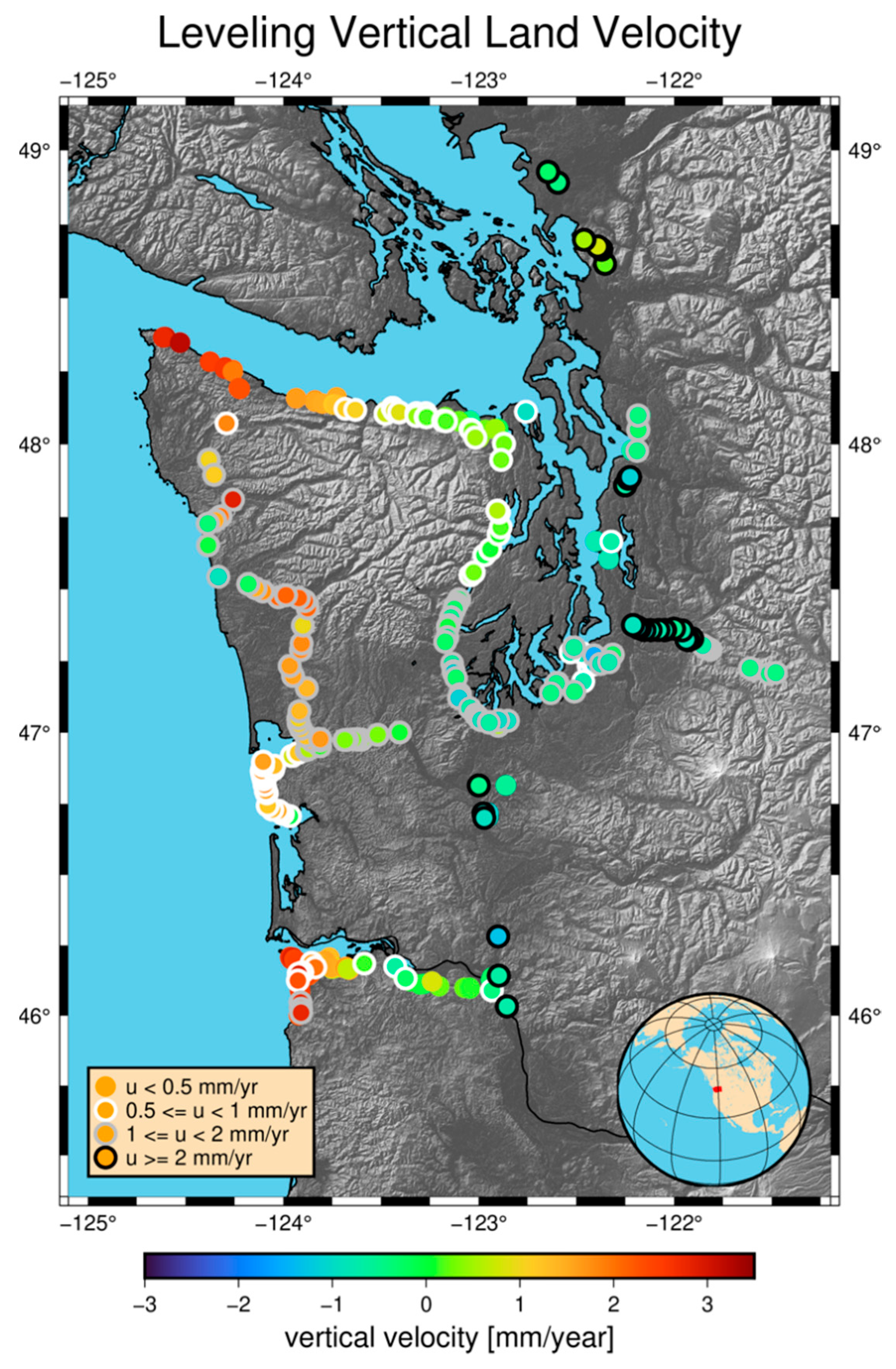
Measurements of vertical land movement derived from leveling. Vertical velocity is denoted by marker color and uncertainty is denoted by marker outline, expressed as millimeters per year (mm/yr). Spatially dense leveling observations perpendicular to the Cascadia subduction zone show the dominant east-west VLM signal resulting from interseismic locking on the megathrust. Refer to Figure 2 for place names. North is up.
Figure 3.
Measurements of vertical land movement derived from leveling. Vertical velocity is denoted by marker color and uncertainty is denoted by marker outline, expressed as millimeters per year (mm/yr). Spatially dense leveling observations perpendicular to the Cascadia subduction zone show the dominant east-west VLM signal resulting from interseismic locking on the megathrust. Refer to Figure 2 for place names. North is up.

Figure 4.
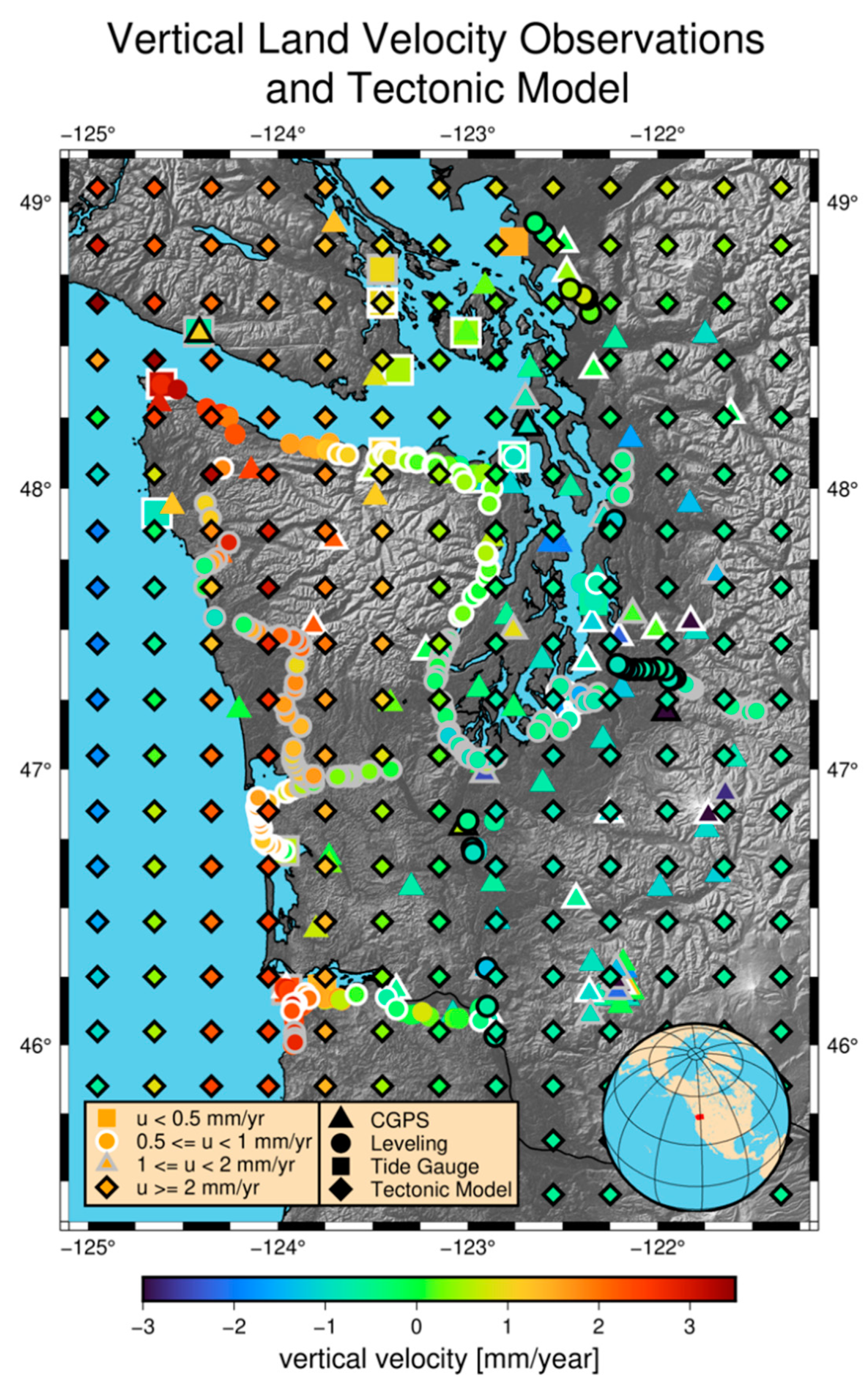
Vertical rate estimates extracted from the tectonic model (Data S1), and measurements of vertical land movement derived from CGNSS, leveling, and tide gauges (Data S2). Data type is denoted by marker shape, vertical velocity is denoted by marker color, and uncertainty is denoted by marker outline, expressed as millimeters per year (mm/yr). We prescribed a conservative uncertainty of 2 mm/year to estimates from the tectonic model. Note the numerous stretches of coastline without VLM measurements. Refer to Figure 2 for place names. North is up.
Figure 4.
Vertical rate estimates extracted from the tectonic model (Data S1), and measurements of vertical land movement derived from CGNSS, leveling, and tide gauges (Data S2). Data type is denoted by marker shape, vertical velocity is denoted by marker color, and uncertainty is denoted by marker outline, expressed as millimeters per year (mm/yr). We prescribed a conservative uncertainty of 2 mm/year to estimates from the tectonic model. Note the numerous stretches of coastline without VLM measurements. Refer to Figure 2 for place names. North is up.

Figure 5.
(a) Interpolated surface queried on a 0.1 degree grid representing a continuous vertical velocity field for coastal Washington (Data S3); (b) Bootstrapped uncertainty of the interpolated vertical velocity field shown in Figure 5a (Data S4). North is up.

Figure 6.
Broad region of coastal subsidence in Washington state along the western Olympic Peninsula. Shown also are vertical rate estimates extracted from the tectonic model, and measurements of vertical land movement derived from CGNSS, leveling, and tide gauges, expressed as millimeters per year (mm/yr). Data type is denoted by marker shape, vertical velocity is denoted by marker color, and uncertainty is denoted by marker outline. North is up.

Figure 7.
(a) Coastal vertical land movements along Washington’s coastline, derived from our interpolant, representing a continuous vertical velocity field for coastal Washington (Figure 5a). Select cities and towns marked by a star and their name in white. (b) Bootstrapped uncertainty of the interpolated vertical velocity field (as shown in Figure 5b) for coastal Washington.

Figure 8.
(a) Three coastal locations in Washington state discussed in: (b) table adapted from Miller et al. [28] showing relative sea level rise projections for 3 of 171 locations along coastal Washington. Projections are expressed in terms of the probability of exceedance for 2100 under two different greenhouse gas scenarios (RCP 4.5 [“Low”] and RCP 8.5 [“High”]; [40]). Projected changes are assessed relative to contemporary sea level, defined as the average sea level over the 19-year period 1991–2009. Projections for all 171 locations are available in [28].

Figure 9.
Relative sea level (RCP 8.5 and a 50% probability of exceedance) over time with and without a hypothetical megathrust rupture at 2070 to exhibit the effect of coseismic land change on relative sea level at La Push, Neah Bay, and Seattle. Coseismic land change is assumed to equal the sum of our estimated annual vertical deformation rate due to the Cascadia subduction zone summed over the hypothetical interseismic period, with the opposite sense of motion. We assume no postseismic viscoelastic relaxation for the purpose of this visualization. The hypothetical earthquake and associated coseismic land changes will produce an instantaneous shift in RSL, and areas experiencing rapid uplift, like Neah Bay, will see a dramatic increase in RSL. Regions that are subsiding west of the zone of interseismic uplift, like La Push, are expected to experience coseismic uplift and will see a decrease in RSL after a major subduction zone earthquake. Regions well east of the subduction zone, such as Puget Sound and Seattle, are expected to experience minor uplift.

Publisher’s Note: MDPI stays neutral with regard to jurisdictional claims in published maps and institutional affiliations. |
© 2021 by the authors. Licensee MDPI, Basel, Switzerland. This article is an open access article distributed under the terms and conditions of the Creative Commons Attribution (CC BY) license (http://creativecommons.org/licenses/by/4.0/).
Share and Cite
MDPI and ACS Style
Newton, T.J.; Weldon, R.; Miller, I.M.; Schmidt, D.; Mauger, G.; Morgan, H.; Grossman, E. An Assessment of Vertical Land Movement to Support Coastal Hazards Planning in Washington State. Water 2021, 13, 281. https://doi.org/10.3390/w13030281
AMA Style
Newton TJ, Weldon R, Miller IM, Schmidt D, Mauger G, Morgan H, Grossman E. An Assessment of Vertical Land Movement to Support Coastal Hazards Planning in Washington State. Water. 2021; 13(3):281. https://doi.org/10.3390/w13030281
Chicago/Turabian StyleNewton, Tyler J., Ray Weldon, Ian M. Miller, David Schmidt, Guillaume Mauger, Harriet Morgan, and Eric Grossman. 2021. "An Assessment of Vertical Land Movement to Support Coastal Hazards Planning in Washington State" Water 13, no. 3: 281. https://doi.org/10.3390/w13030281
Note that from the first issue of 2016, this journal uses article numbers instead of page numbers. See further details here.