
Flow Turbulence Characteristics and Mass Transport in the Near-Wake Region of an Aquaculture Cage Net Panel


1
State Key Laboratory of Water Environment Simulation, School of Environment, Beijing Normal University, Beijing 100875, China
2
Tang Scholar, Beijing Normal University, Beijing 100875, China
3
School of Science and Engineering, University of Dundee, Dundee DD1 4HN, UK
4
Department of Civil and Environmental Engineering, Rutgers, The State University of New Jersey, Piscataway, NJ 08854, USA
5
Department of Civil, Architectural and Environmental Engineering, University of Naples Federico II, 80125 Napoli, Italy
*
Authors to whom correspondence should be addressed.
Water 2021, 13(3), 294; https://doi.org/10.3390/w13030294
Submission received: 21 December 2020
/
Revised: 19 January 2021
/
Accepted: 21 January 2021
/
Published: 25 January 2021
(This article belongs to the Special Issue Advances in Environmental Hydraulics)
Abstract
:Cage-based aquaculture has been growing rapidly in recent years. In some locations, cage-based aquaculture has resulted in the clustering of large quantities of cages in fish farms located in inland lakes or reservoirs and coastal embayments or fjords, significantly affecting flow and mass transport in the surrounding waters. Existing studies have focused primarily on the macro-scale flow blockage effects of fish cages, and the complex wake flow and associated near-field mass transport in the presence of the cages remain largely unclear. As a first step toward resolving this knowledge gap, this study employed the combined Particle Image Velocimetry and Planar Laser Induced Fluorescence (PIV-PLIF) flow imaging technique to measure turbulence characteristics and associated mass transport in the near wake of a steady current through an aquaculture cage net panel in parametric flume experiments. In the near-wake region, defined as ~3M (mesh size) downstream of the net, the flow turbulence was observed to be highly inhomogeneous and anisotropic in nature. Further downstream, the turbulent intensity followed a power-law decay after the turbulence production region, albeit with a decay exponent much smaller than reported values for analogous grid-generated turbulence. Overall, the presence of the net panel slightly enhanced the lateral spreading of the scalar plume, but the lateral distribution of the scalar concentration, concentration fluctuation and transverse turbulent scalar flux exhibited self-similarity from the near-wake region where the flow was still strongly inhomogeneous. The apparent turbulent diffusivity estimated from the gross plume parameters was found to be in reasonable agreement with the Taylor diffusivity calculated as the product of the transverse velocity fluctuation and integral length scale, even when the plume development was still transitioning from a turbulent-convective to turbulent-diffusive regime. The findings of this study provide references to the near-field scalar transport of fish cages, which has important implications in the assessment of the environmental impacts and environmental carrying capacity of cage-based aquaculture.
1. Introduction
The fast-growing aquaculture industry is challenged by a number of environmental concerns, such as nutrient and waste dispersion [1], disease spreading [2], and sea floor deterioration below the farms [3]. As a key forcing factor that drives the transport of nutrients, dissolved oxygen, waste, and pathogens in the vicinity of the farm, the ambient flow field is critical to the efficient functioning of the fish farm as well as to its potential environmental impacts. If the ambient flow is generally subject to local hydrographic conditions, in fish farms located in inland lakes or reservoirs and coastal embayments or fjords, the cages are subjected to time-varying flows driven by wind and tides, which can be modified significantly by the presence of the aquaculture cage structures due to their partial blockage of the flow [4]. On the regional scale, the altered hydrodynamic conditions may further affect sediment transport pathways and coastal erosion, etc., contributing to the loss of habitat of sensitive species and thus the biodiversity and ecosystem services they sustain [5]. As a key component of fish cages, the net panels are porous and highly flexible structures made up from a large number of small intersecting circular cylinders (e.g., nylon twine), and the flow field through and around this arrangement is rather complex. In aquaculture practice, the flow field through the cages affects water exchange and thus the transport of oxygen, nutrients, waste, pathogens, etc., in the water column, which further affects fish health and growth and the surrounding environment. To enable accurate assessment of environmental impact and regulation compliance in order to achieve environmentally sustainable aquaculture, it is imperative to elucidate the near-field turbulent flow and mass transport processes through the aquaculture cage net panel.
Flows through and around screens and gauzes that are similar to fishing net occur in a wide range of engineering applications, including flow-manipulating screens used in wind tunnels [6], fish screens installed before water intakes [7], and insect screens associated with greenhouse ventilators [8]. The presence of such structures in flow is well known to cause significant effects on the through-flow characteristics, such as pressure drops, velocity reductions, and deflections of streamlines. These effects were found to be dependent on the properties of the net structure, including the rigidity, porosity (or solidity), inclination to the main flow direction, and the incoming velocity [4,6]. Specific to the effects of fishing nets on the time-averaged through-flow, Bi et al. [9] measured the flow velocity downstream of a fishing net in a steady current using Particle Image Velocimetry (PIV) and Acoustic Doppler Velocimeter (ADV) and found a clear reduction downstream of the plane net that increased with increasing net solidity and net inclination angle to the flow.
For the analogous classic topic of grid-generated turbulence, which has been extensively studied, Batchelor [10] suggested that the region just downstream of the grids where the flow is highly inhomogeneous and grid geometry dependent, i.e., the near field, extends downstream to , where x is the downstream distance from the grid and M is the grid mesh size. Within the near field, the turbulence initially increases and then decays, corresponding to the production and decay regions, respectively. It is well established that the turbulence intensity follows a power-law decay in decaying grid-generated turbulence [11,12]. More recently, Isaza et al. [13] confirmed that turbulence energy decayed more rapidly in the near field than in the far field. Whereas the majority of the grid turbulence studies that have aimed to generate homogeneous and isotropic turbulence have been based on wind-tunnel experiments, Cardesa et al. [14] measured turbulence statistics immediately downstream of two different biplanar regular grids made of circular and square rods in open-channel flows using PIV. Gan and Krogstad [15] further conducted PIV measurement on the near-field wakes behind monoplane square grids of both regular and multiscale types. A number of studies have also investigated the structure of turbulence generated by oscillating grids in otherwise quiescent ambient water bodies, e.g., [16,17,18], indicating a power-law decay in turbulence intensity with increasing distance from the mid-plane of grid oscillation.
Compared to the effects of the presence of net structures on the turbulent flow field, their influence on the scalar transport has been much less studied. Among the few available studies, Nakamura et al. [19] performed separate measurements of velocity and concentration fields, as well as theoretical analysis of the cross-correlation between concentration and velocity fluctuations, to study mass diffusion in grid-generated turbulence. Subsequently, an experimental measurement of turbulent scalar flux and turbulent diffusivity was performed in scalar transport from a point source into grid turbulence by Lemoine et al. [20] using combined LIF and LDV. Also, Cuthbertson et al. [21] investigated the structural development and breakdown of turbulent, round buoyant jets resulting from their interaction with a turbulence patch generated by an oscillating grid. Their experimental results indicated that the jet breakdown location was determined primarily by the relative magnitude of turbulent velocities in the patch and jet, scaling successfully with limiting cases of momentum- and buoyancy-dominated regions of the buoyant jet. More recently, Nedic and Tavoularis [22] studied the diffusion of heat injected from a line source into turbulence generated by regular and fractal square grids in the near-wake region and investigated the dependence of mixing performance on grid geometry and relative location of the source. The turbulent diffusivities were found to agree with Taylor’s [23] theory of diffusion and correlate with the transverse turbulence intensity and integral length scale.
It is worth pointing out that the above studies have mainly focused on grid-generated turbulence and its effects on the flow field. For the limited studies on the scalar transport from a point source into grid turbulence, their sources were mostly located downstream of the grid and the measurement range was also far downstream of the grid. In addition to the grid-generated homogenous and isotropic turbulence studies, as far as we are aware, studies on the turbulence characteristics and near-field mass transport of flow through net or grid structures, particularly those mimicking aquaculture cage nets, are generally lacking, despite an inadequate consideration of the wake on the net panel could lead to inaccurate predictions in fish cage models [4]. Hence, the main objective of this experimental study was to explore the turbulence characteristics and mass transport generated in the near wake of a model fishing net panel. Panels with different geometric properties were placed vertically across the entire channel cross-section, perpendicular to the mean approaching flow direction (i.e., representative of an infinite net tested under steady currents in which the mean streamwise current velocity was varied as an experimental parameter). Two-dimensional horizontal velocity and concentration fields were measured using combined Particle Image Velocimetry and Planar Laser Induced Fluorescence (PIV-PLIF) at locations far away from flume boundary. The results presented herein provide references for further study of the wake flow and near-field mass transport processes associated with cage-based aquaculture.
2. Methodology
2.1. Experimental Setup and Instrumentation
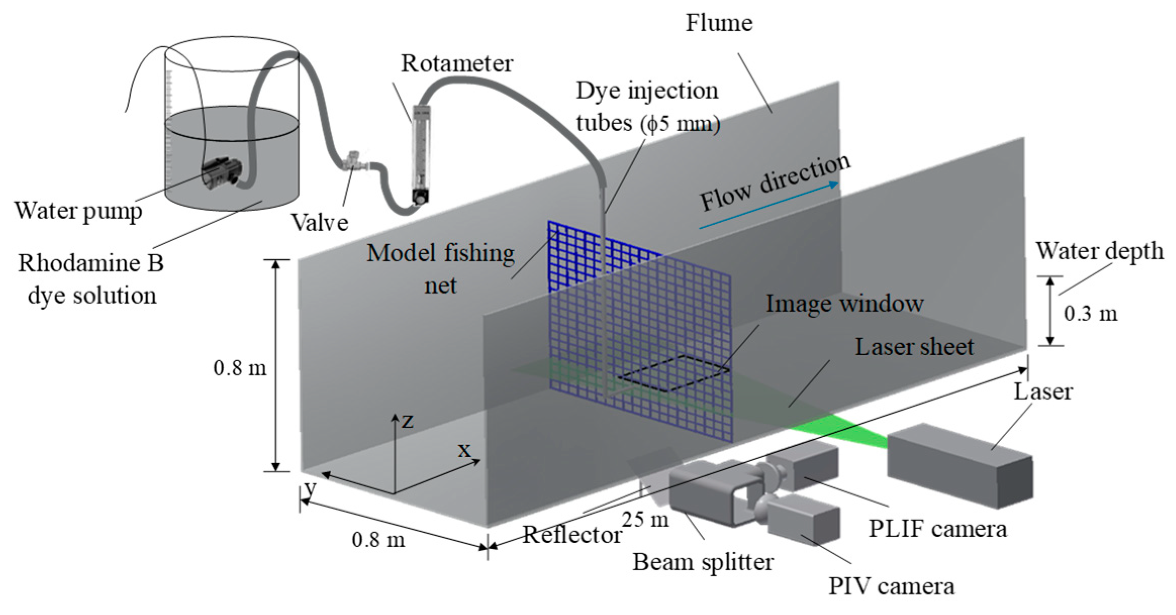
The experiments were conducted at the State Key Laboratory of Water Environment Simulation at Beijing Normal University. Figure 1 shows a schematic diagram of the experimental setup and the coordinate system. The recirculating flume measured 25 m (length) by 0.8 m (width) by 0.8 m (height), with a maximum flow rate of 240 L/s. Fully developed, uniform open-channel flow was generated in the recirculating flume by a pump located at one end of the flume, with different current velocities obtained by changing the operational frequency of the pump. The water depth (h) was fixed at 0.3 m. The test section was located at the middle of the flume 10 m downstream of the flume entrance. Model net panels made from polyethylene netting were stretched tightly and fixed on a square steel frame with 4 mm diameter strings such that the net deformation in flowing water was negligible. The net panel was then placed perpendicular to the flume side walls, occupying the entire channel cross section to eliminate the effects of free ends. A fluorescent dye, Rhodamine B, was used as a passive tracer to study the near-field mass transport process through the net panel, with 6.5 mg/L Rhodamine B solution injected continuously through a 5 mm diameter nozzle as a point source placed 20 cm upstream of the net. The center of the nozzle was aligned to the flume centerline at the mid-depth plane (i.e., 0.15 m above the flume bed). The dye injection flow rate was measured by a rotameter and adjusted with a built-in valve to match the ambient current velocity (i.e., representing a passive and isokinetic source condition). x, y, and z denote longitudinal, transverse, and vertical coordinates, respectively, and the origin of the coordinate system was set at the location of the net along the centerline of the flume at mid-depth.
A combined PIV-PLIF technique was used in this study for quantitative velocity and concentration measurements of the near-wake region immediately downstream of the net panel. Flow seeding was provided by natural impurities in the water for PIV measurement, and Rhodamine B was adopted as the fluorescent (passive) dye tracer for PLIF measurement. A Vlite-200 dual-cavity Nd: YAG pulsed laser (15 Hz, 200 mL, 532 nm, Beam tech, Beijing, China) was placed beside the flume to produce a horizontal light sheet with a thickness of 1.5 mm. The light sheet cut through the centers of the net meshes around mid-depth to illuminate the measurement area. Two Speed Sense M120 high-speed cameras (1920 × 1200 pixels resolution, maximum frame rate 730 fps, Dan tec Dynamics) were used to capture the images for PIV and PLIF. The two cameras were mounted at right angle on a dual camera mount and captured the same field-of-view (FoV) through beam splitter optics. This camera arrangement was set on a horizontal traverse system below the flume, allowing fine adjustment of the camera positions. The cameras were positioned such that the FoVs were symmetrical about the flume centerline and focused toward the laser illumination plane. Both cameras were fitted with 50 mm f/1.8 Nikkor lenses, and the PIV and PLIF cameras were fitted with 532 nm band-pass and 570 nm low-pass filters, respectively.
2.2. Experimental Procedures
First, scale calibration was made by a standard target of 200 mm × 200 mm, which was followed by image dewarping performed on the instantaneous PIV and PLIF images using multicamera calibration in the Dynamics Studio software (Dantec Dynamics, Denmark) to maximize the coincidence of the two images. The resultant measurement area was 300 × 190 mm2, and the associated resolution was 0.173 mm per pixel. A maximum laser pulse repetition rate of 15 Hz was used, while the pulse duration and time interval between pulses were set at 8 ns and 2700 μs after being optimized for the current PIV measurement. The PLIF images were acquired from the first frame of the double exposures. The instantaneous PIV images were analyzed using the adaptive cross-correlation algorithm in Dynamics Studio, with a final interrogation area (IA) of 32 × 32 pixels with three refinement steps and 33.3% overlap, yielding a 57 × 36 vector field for each instantaneous image. Spurious vectors were removed by range validation and replaced by interpolation. In all cases, the number of replaced vectors was less than 3% of the total number. Pixel-by-pixel calibrations were required for quantitative PLIF measurements before each experiment, in which least-square fitting was performed to relate the grayscale value in the captured images of a number of calibration solutions to the known dye concentration in these solutions. Specifically, a small acrylic tank was placed inside the flume at the location of the FoV with its side walls parallel/perpendicular to the flume side walls. It was filled with uniform Rhodamine B solution with varying concentrations, namely 0 ug/L, 30 ug/L, 60 ug/L, 90 ug/L, and 120 ug/L, and the flume was filled with water to the same level. Once the calibration was completed, the laser and camera settings were kept unchanged throughout the entire experiment. The test section was covered by a black curtain to eliminate the disturbance of background light.
Based on the similitude in net solidity between model and prototype fishing nets and the experimental parameters adopted in relevant previous studies [9,24,25,26], two model nets and two current velocities (i.e., 0.290 m/s and 0.142 m/s) were tested in this study. A control case in the absence of the net panel was also conducted. The experimental parameters, including the net geometric properties and flow conditions, are documented in Table 1. Notably, Løland [27] proposed that the interactions between the wakes generated by the individual twines can be neglected when M/d > 5–6, where d is the diameter of the net twine. This condition is generally satisfied in the present experimental configuration, except near the intersections where the twines cross each other. Net solidity S, which is defined as the ratio between the projected area of the net panel (i.e., the part that blocks the flow) and the total area enclosed by the net panel, is also an important dimensionless parameter characterizing the net geometric properties. For the knotless nets with square mesh used in this study, the net solidity S can be calculated as .
For a typical experimental run, the sampling frequency was set at 15 Hz over a duration of 100 s, during which 1500 PIV and PLIF images were captured to allow time-average and statistical turbulence analysis, and the statistical convergence of the measured quantities was ensured. Once the flow current with the desired velocity U0 was established and stabilized along the flume channel, the dye injection was switched on, and simultaneous PIV and PLIF data acquisition were initiated after the dye tracer plume was stabilized at the measurement area. The downstream extent of the measurement region in the various tests was 300 mm, which fell well within the near-wake region (i.e., ).
3. Results and Discussion
3.1. Time-Averaged Velocity and Concentration Field
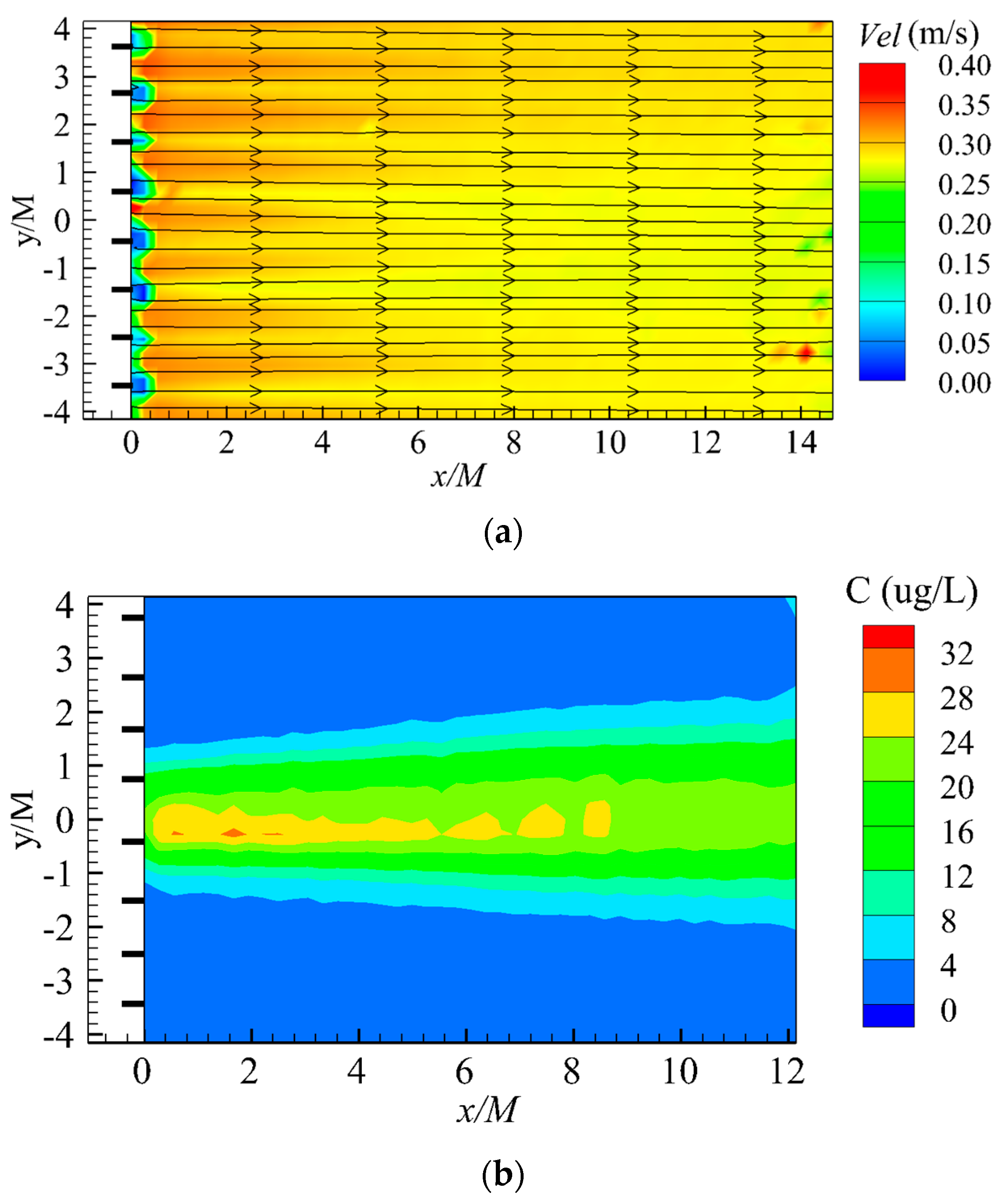
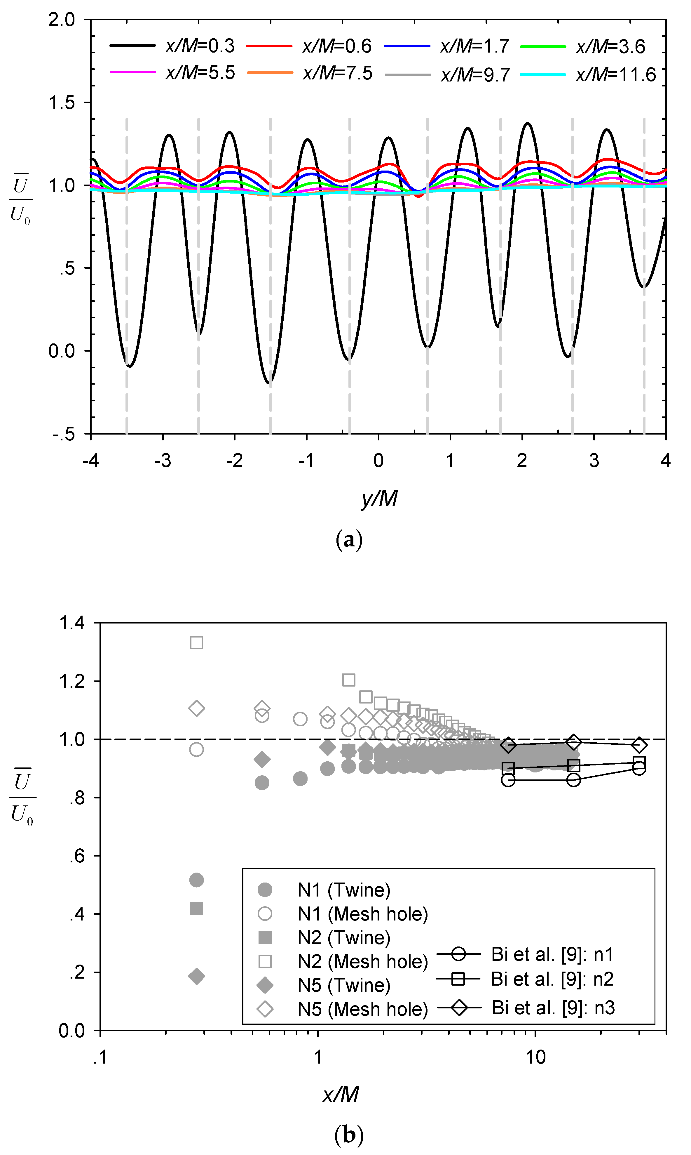
The synoptic, time-averaged velocity fields downstream of the net panel for the representative case N5 (generally used in the following discussions, unless otherwise specified) are shown in Figure 2a. The longitudinal and lateral coordinates were normalized by the mesh size M. The streamlines show the flow direction through the nets, whereas the velocity magnitude is shown by the graded color contour map. As shown by the color mapping, the current velocities were blocked at the periodically spaced vertical twines (their locations are marked by the black bars shown in Figure 2a), and locally increased velocities in the net mesh (or hole) between these twines, resulting in initial periodic peaks and troughs in velocity immediately downstream of the net panel. The ratio of velocity reduction (the ratio between the wake velocity and the incoming velocity U0) is commonly used to measure the effects of flow blockage of net structure [4]. The periodicity of the velocity fluctuation behind the net is clearly illustrated by the lateral profiles of the normalized velocity in Figure 3a (the gray dashed lines marking the location of the twines), which decays steadily in the downstream direction (i.e., increasing x/M), with the mean velocity becoming more homogeneous and recovering to the incoming velocity (i.e., . Recirculation (i.e., ) was virtually suppressed directly behind the twines at the center-of-mesh measurement plane as observed previously [15].
The ratio of the mean streamwise velocity to the incoming velocity at different longitudinal distance x/M behind the central twine and the adjacent mesh hole for the various cases (Table 1) are shown by the unconnected grey symbols in Figure 3b. The results from Bi et al. [9] (connected black symbols) are also included in the figure for comparison. The initial reduction of the velocity behind the twines (x/M~0.3) and the subsequent gradual recovery of the incoming velocity as x/M increases is clearly shown, while velocities at the mesh hole locations exhibited opposite trend of variation and appeared to approach the incoming velocity at a slower rate (i.e., over greater x/M). Similar trends with wider contrast between bar and hole locations were also reported in Gan and Krogstad [15] for wake flow generated behind a grid with a larger solidity ratio and higher incoming velocity. Notably, the velocity recovery (i.e., to ) was incomplete within the x/M range of our measurements, which is consistent with Bi et al. [9]. Among the different cases, the magnitude of the incoming velocity appeared to affect the ratio of velocity reduction (augmentation) more significantly than the net solidity in our experimental coverage, e.g., comparing N1 (same S but smaller U0) with N2 and N2 with N5 (same U0 but smaller S) in Figure 3b. Moreover, the net solidity of case N1 in the present study was comparable with cases investigated by Bi et al. [9] (residing between reference cases n2 and n3) with a similar incoming velocity, resulting in the associated ratio of velocity reduction also residing between these two reference cases.
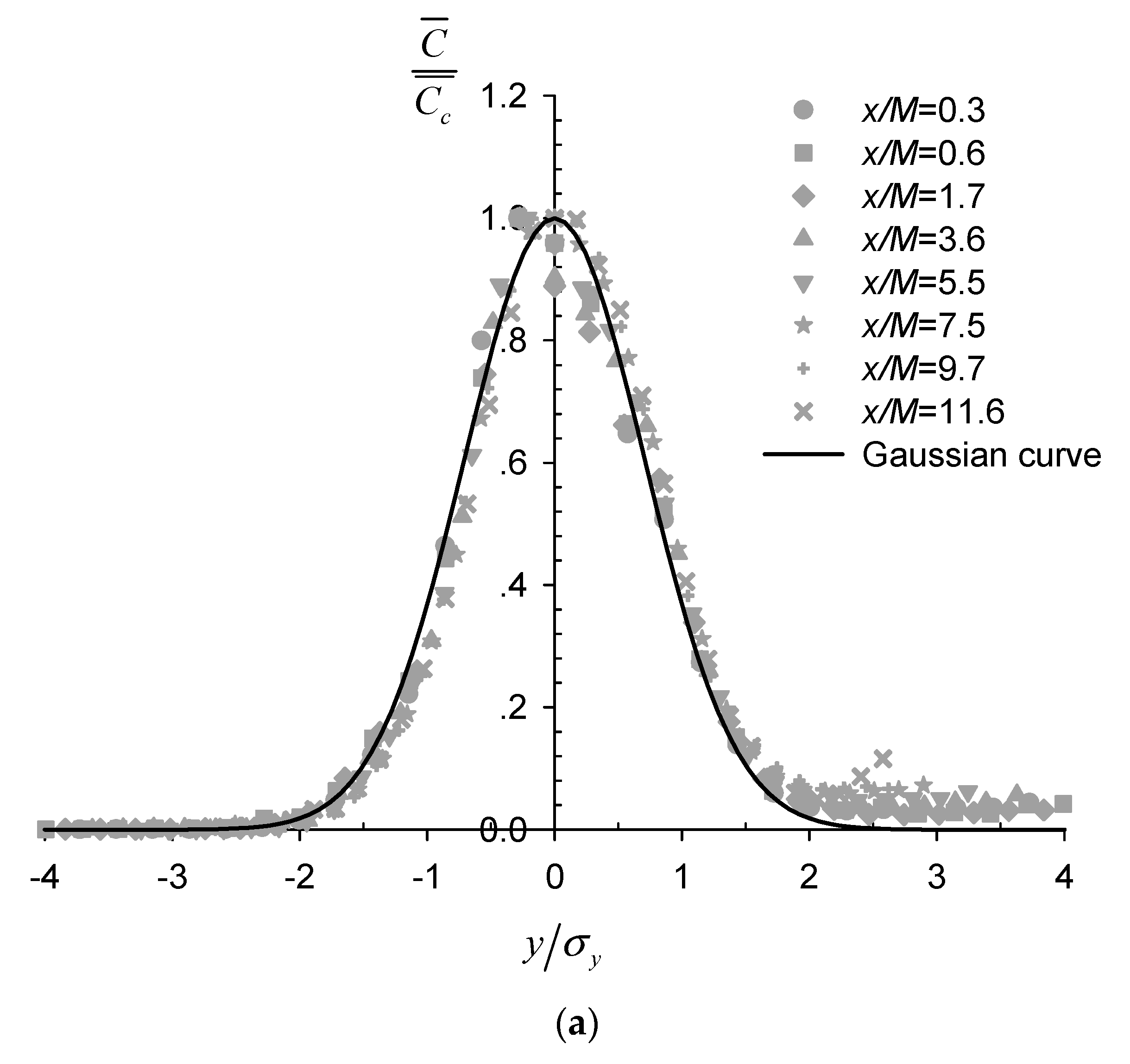
The time-averaged concentration field for case N5 is shown in Figure 2b. The coordinates were normalized by the mesh size M, and the twine locations are marked by the black bar as in Figure 2a. Within Figure 2b, a quasi-symmetrical plume was generated about the central axis (y/M = 0), as evident from the concentration contours, which were mostly smooth except along the core at the centerline. This plume was shown to expand approximately linearly in width with increasing distance x/M downstream of the net panel. The lateral profiles of the normalized time-averaged concentration at various downstream locations are shown in Figure 4a to be well fitted with Gaussian functions, such that
where is the time-averaged concentration at location , is the concentration at the plume centerline, is the standard deviation in the transverse direction representing the spreading width of the scalar plume. The lateral concentration profile appears to follow Gaussian distribution regardless of the presence of the nets, even at the closest downstream location to the net panel of x/M = 0.3, with the strongly inhomogeneous wake flow field (Figure 2a and Figure 3a). This is consistent with reported Gaussian passive scalar plumes downstream of point sources in well-established homogeneous and isotropic grid turbulence [19,28]. Notably, Lemoine et al. [29] also reported self-similar Gaussian profiles of transverse concentration distribution at locations closer to the grid where the turbulence field still exhibited inhomogeneity.
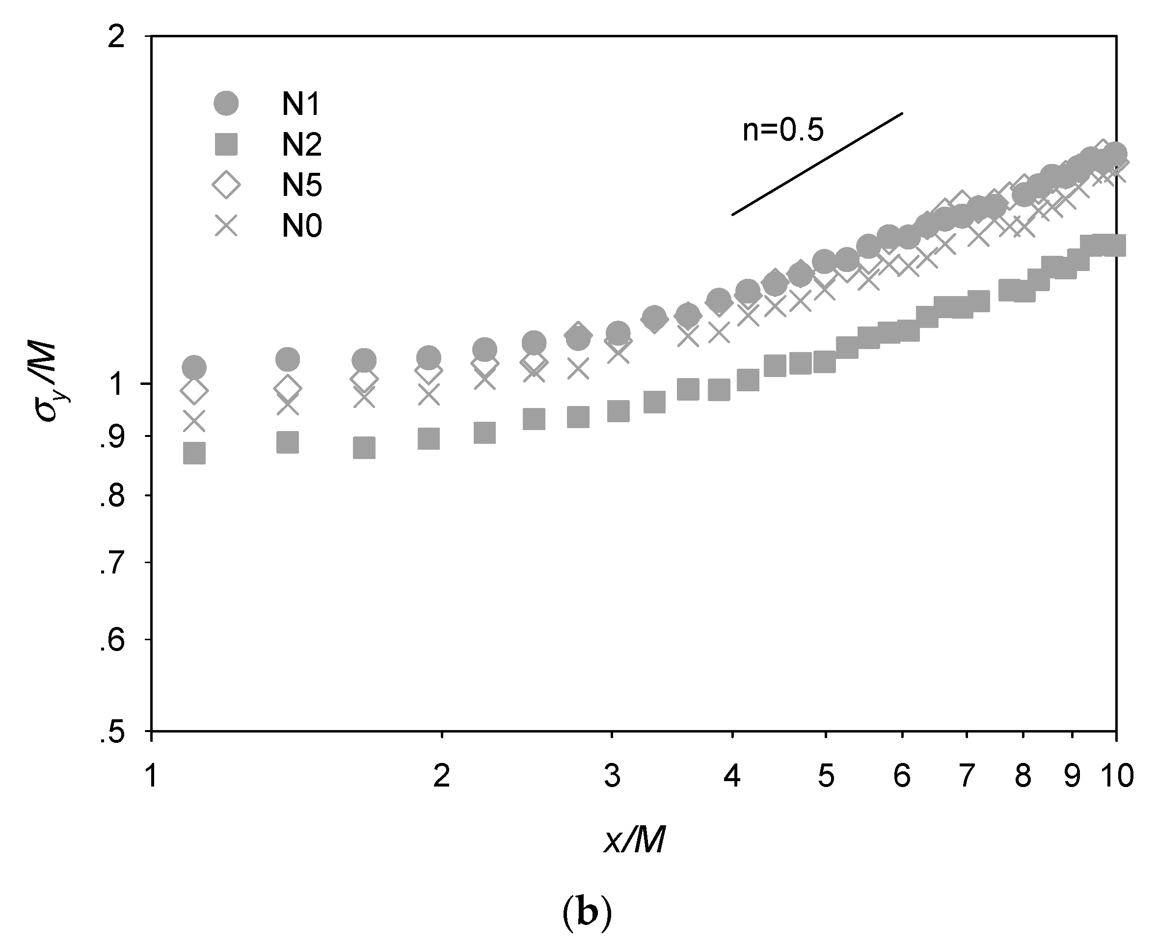
The evolution of the measured spreading width with downstream distance for the various cases is presented in Figure 4b. Comparison among the various cases, including the no-net case N0, suggests that, except for case N2 which also exhibited reduced transverse integral length scale (discussed later), the presence of the net slightly enhanced the lateral spreading of the plume. According to Taylor’s diffusion theory, when the plume spreading width becomes sufficiently larger than the integral length scale of the flow, i.e., the plume development enters the turbulent-diffusive regime, it scales with the downstream distance as follows [19,22],
where D denotes the turbulent diffusivity or Taylor diffusivity. A linear growth pattern of the plume spreading width is discernable on logarithmic scale for x/M > ~4. However, the slope was still lower than 0.5 (i.e., as dictated by Equation (2)), consistent with the previous finding that the plume width started to follow the square root law from x/M = 13 in grid turbulence [29].
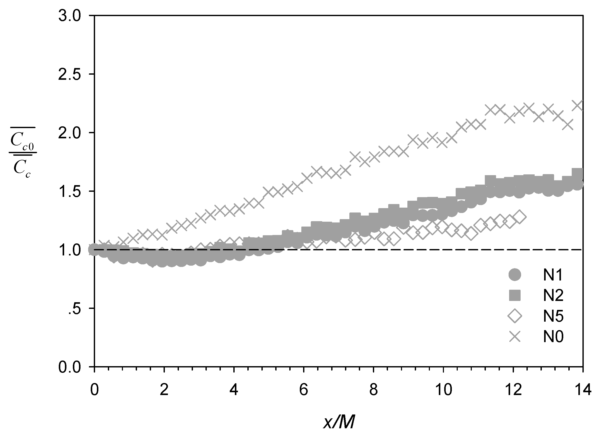
The longitudinal profiles of the inverse of scalar concentration along the plume centerline normalized by the mean concentration at the net panels, , are shown in Figure 5. In contrast to the no-net case N0, which showed a steady (and approximately linear) concentration decrease between x/M = 0 to ~11, the corresponding profiles with net panels showed a slight increase (i.e., < 1) immediately downstream the net followed by steady decrease (i.e., increasing), with the demarcation corroborating approximately with regions of turbulence production (x/M < ~3) and decay (x/M > ~3) (see Figure 6a). Lemoine et al. [29] also reported a change of slope at x/M ~ 10, after which exhibited linear growth with downstream distance, as expected for scalar transport in homogeneous and isotropic grid turbulence [19]. Another contrast is also evident further downstream between N1 and N2 (filled symbols) with the plume centerline close to net twine versus N5 (unfilled symbols) with the plume centerline aligned in the mesh hole.
3.2. Turbulence Characteristics
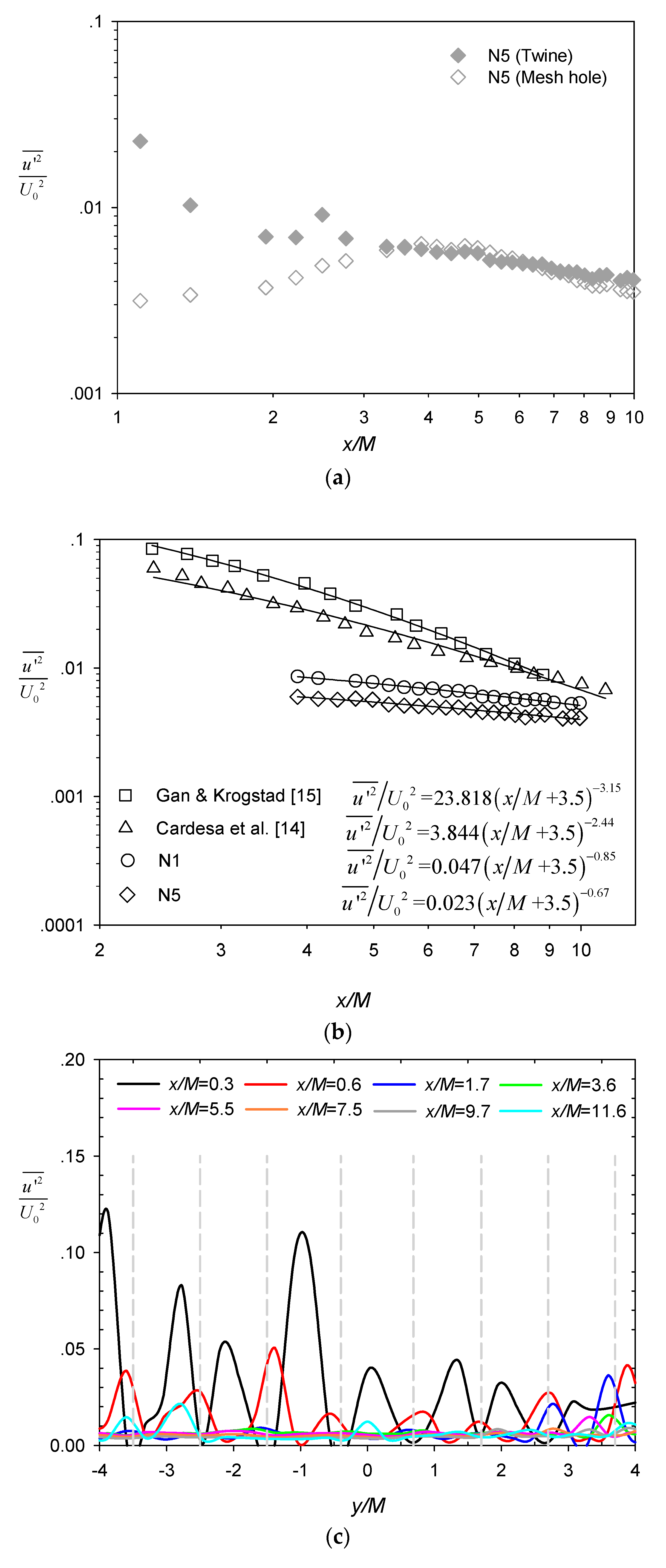
Figure 6a presents the longitudinal evolution of streamwise turbulence intensity behind the central twine (filled symbols) and the adjacent mesh hole (unfilled symbols) for test case N5. Close to the net, the turbulence intensity behind the twine was significantly larger than measured at the mesh hole, with the former exhibiting two peaks (at x/M = ~1 and ~2.5) and the latter exhibiting a single peak (at x/M ~ 4). This is consistent with the patterns reported by Gan and Krogstad [15]. After x/M ~ 3, the two profiles tended to collapse and largely follow a decaying trend [14]. It is well established that the turbulence intensity follows a power-law decay in decaying grid-generated turbulence [11,12],
where u’ is velocity fluctuation, overbar denotes time average, n is the decay rate, a is a constant, and x0 is the virtual origin. This power-law decay was manifested by the straight-line portion in the range of x/M = ~4 to ~10 in the log-log plot shown in Figure 6a. Several previous studies [13,22] have also reported more rapid decay (i.e., larger n in Equation (3)) in the developing (near-field) region than the fully developed (far-field) region of decaying grid turbulence. Furthermore, Isaza et al. [13] observed that the near-field decay region extended to x/M ~ 12. Therefore, the power decay region in this study fell within the near-field decay region. Assuming x0 = −3.5M is used in Equation (3) for the near-field decay region [22], n and a were fitted for the power decay region behind the twine for N1 and N5 in Figure 6b and documented in Table 2. Given the sensitivity of the curve fits to the setting of virtual origin for relatively narrow range of measurement, we also fitted alternative power functions to the same data under the assumption of x0 = 0 [11,13]. Regardless, the range of n values determined in the present study was much smaller than those reported from wind-tunnel experiments [13,22] and a previous water-channel experiment [19]. Although Gan and Krogstad [15] argued that the power-law decay region was not yet attained in their water flume measurements, the turbulence intensity and the slope of decay reported in their study, as well as those of Cardesa et al. [14], were significantly larger than in the current study (Figure 6b). The discrepancy among the various studies is mainly due to the net properties (e.g., mesh size, twine diameter, and rigidity) and working fluid (i.e., air versus water), which dictate the development of the turbulence [11]. Moreover, the elevated turbulence intensity in N1 relative to N5 shown in Figure 6b is also consistent with the finding of Ito et al. [30]. Given the same mesh size, the turbulence intensity increased with grid bar (or net twine) thickness.
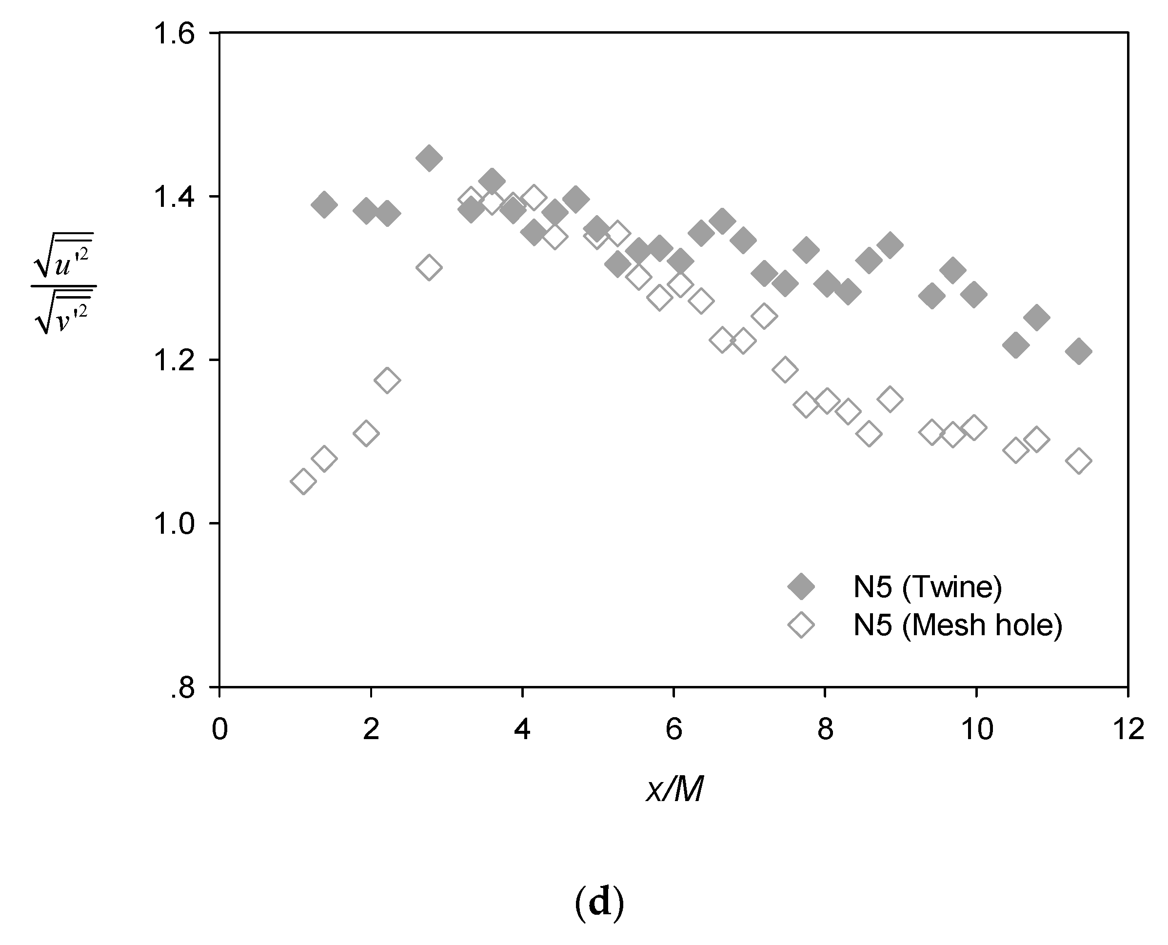
The lateral profiles of the streamwise turbulence intensity for N5 (Figure 6c) also shows that the turbulence decayed and, at the same time, became more homogeneous with increasing downstream distance x/M from the net panel. Similar to the observation by Gan and Krogstad [15], the local peaks were positioned within the strong shear regions and were slightly offset from the twine location (shown as dashed grey lines). Figure 6d shows the longitudinal profile of the turbulence anisotropy ratio, i.e., behind the twine (filled symbols) and at the mesh hole (unfilled symbols) for test case N5. It is noted here that the anisotropy ratio was greater than unity throughout the x/M measurement range, suggesting that isotropic turbulence was not developed in this region, while the anisotropy ratio was generally larger behind the twine than at the mesh hole.
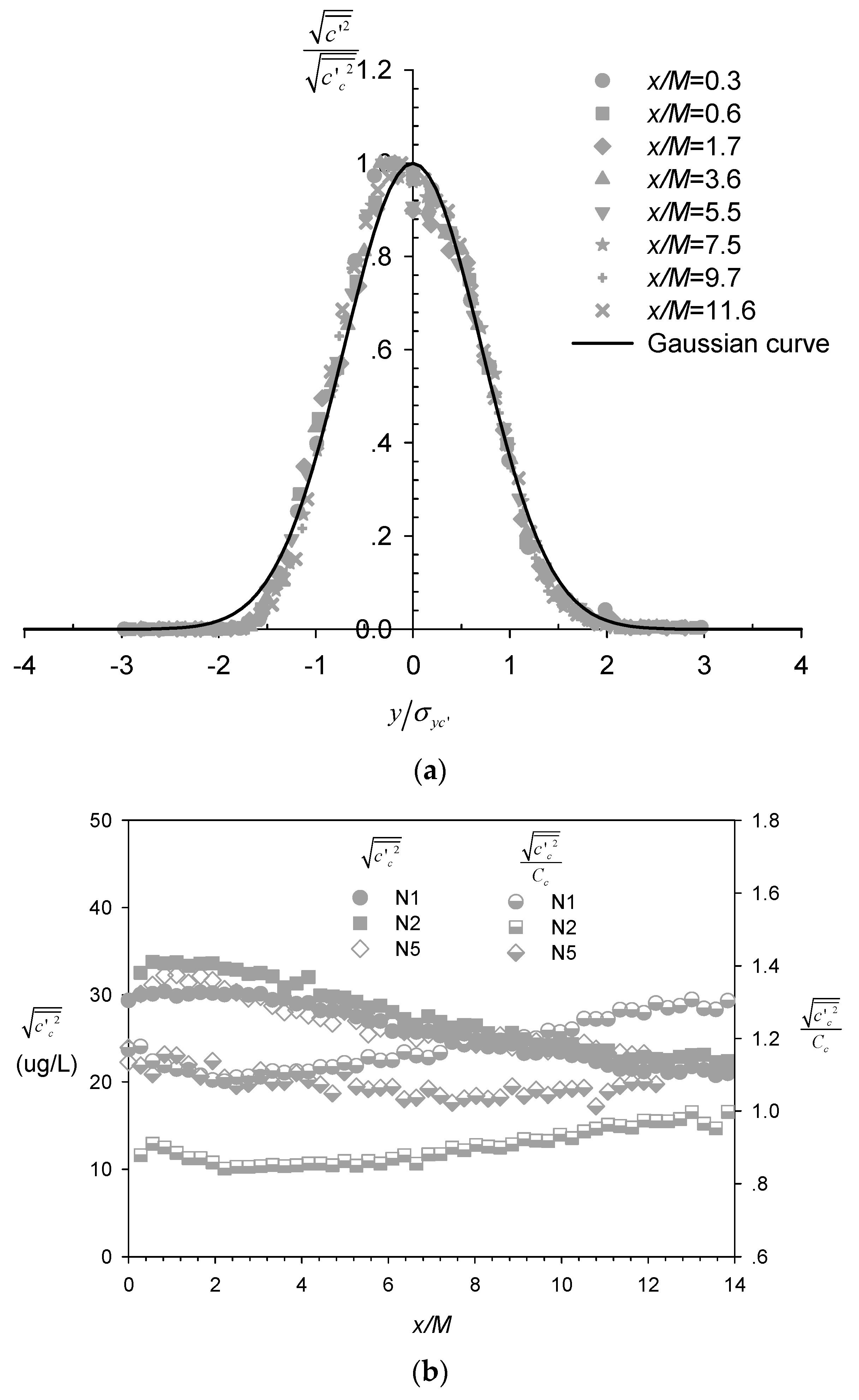
Figure 7a shows the lateral profiles of the root mean square (RMS) of the concentration fluctuation normalized by the local centerline value . These profiles were very similar at all x/M locations and followed a Gaussian distribution reasonably well, as reported previously for scalar plumes arising from point source in grid turbulence [28]. Notably, the fitted standard deviation that characterized the spreading width of the concentration fluctuations was much larger than its counterpart, which was related to the mean concentration . Figure 7b shows the longitudinal, centerline evolution of the RM) of the concentration fluctuation (filled and unfilled symbols) and their ratio with time-averaged concentration (half-filled symbols). In general, the values exhibited a steady decrease with increasing downstream distance (i.e., for x/M > ~2–3). By contrast, while values for profiles of N1 and N2 taken behind the twine showed a slight increase further downstream (i.e., x/M > ~3), as reported by Nakamura et al. [19], the profile of N5 taken at the mesh hole decreased monotonically with distance before approaching an asymptotic value around unity for x/M > ~6. This is significantly larger than reported asymptotic values for scalar line plumes generated in grid turbulence in wind tunnel, which were found to vary in the wide range of 0.25–0.7 [22].
3.3. Turbulent Mass Transport
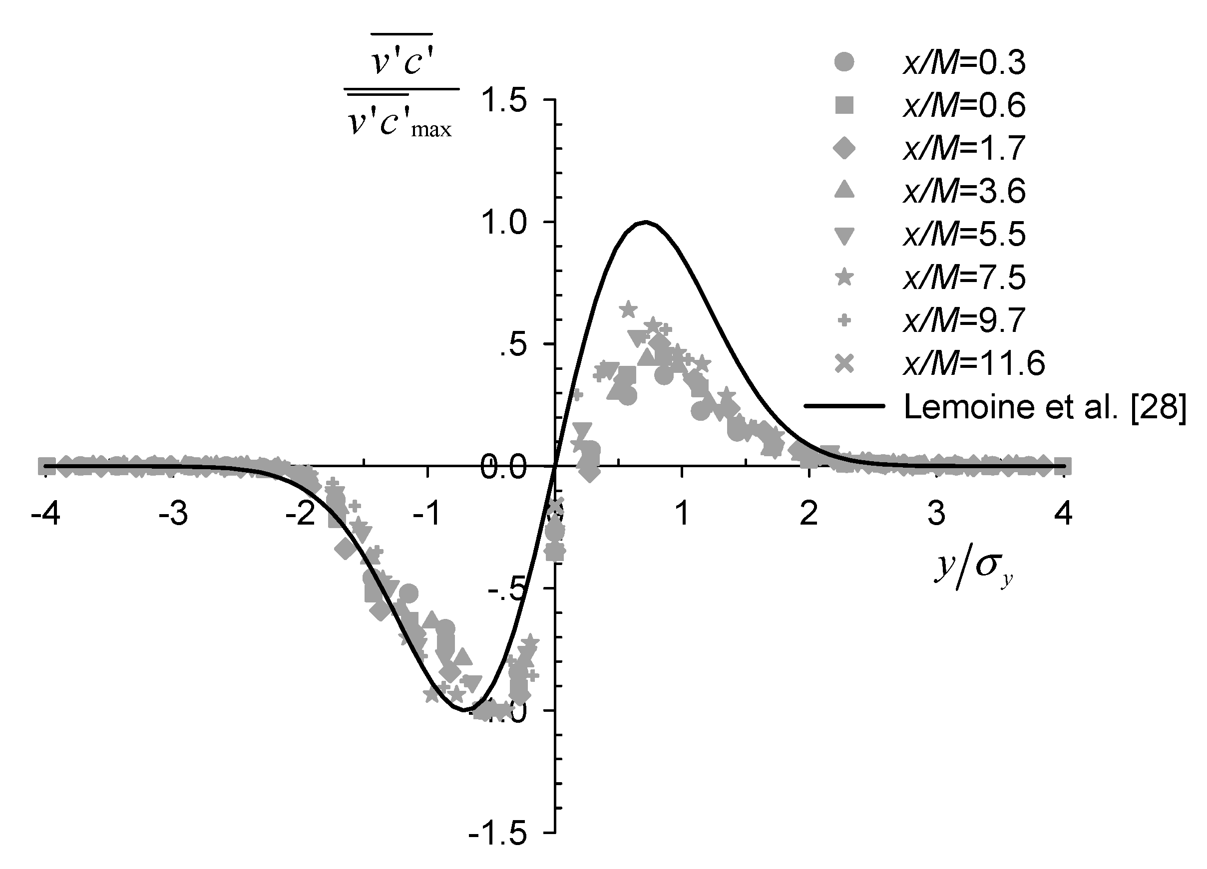
Simultaneous measurements of instantaneous velocity and concentration data allowed us to calculate their correlation and analyze the turbulent scalar flux, which is an important parameter that quantifies the turbulent mass transport. Figure 8 shows the lateral profiles of the transverse turbulent flux normalized by their maximum at each section. The profiles were nearly self-similar and antisymmetric about the centerline, as reported previously for axisymmetric scalar plumes from point source in grid turbulence [28]. However, deviation from the theoretical curve , developed by Lemoine et al. [28] assuming self-similarity and the gradient-diffusion hypothesis, was still evident, especially in the positive region. This suggests that the two assumptions were not entirely satisfied within the current experimental range.
It is well established that the development of the scalar plume in grid turbulence generally consists of three regimes, namely the molecular-diffusive regime, the turbulent-convective regime and the turbulent-diffusive regime [22,31]. The molecular-diffusive regime corresponds to the very near-source region, during which the size of the plume is extremely small, and its spreading is due to molecular diffusion only. As the plume grows, it remains significantly narrower than the integral length scale of the turbulence, and the transverse velocity fluctuations dictate its spreading rate (i.e., the turbulent-convective regime). When the plume spreading width becomes sufficiently larger than the integral length scale, it enters the turbulent-diffusive regime.
The integral length scale of transverse velocity fluctuations Lt represents the characteristic size of large-scale eddies that drive the turbulent diffusion of the passive scalar, and can be written in the form
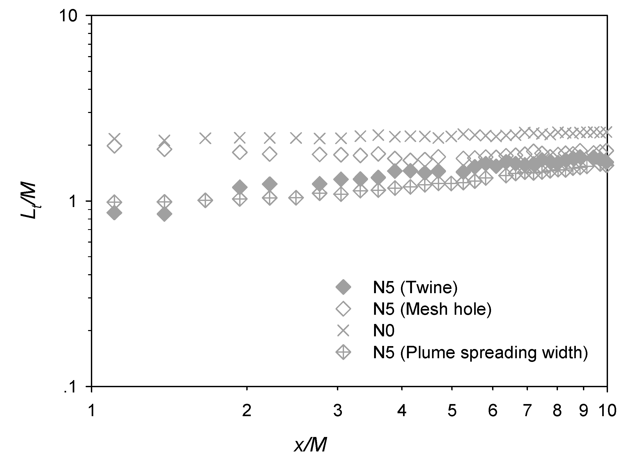
where ey is the transverse unit vector and r is the separation [15,22]. The longitudinal development of the normalized transverse integral length scale Lt/M for test case N5 is shown in Figure 9. This shows that, while Lt/M at the mesh hole was consistently greater than the corresponding value behind the twine (i.e., at all x/M), the two profiles tended to approach each other at more downstream locations (i.e., x/M > ~5). Corresponding to the power-law decay of the turbulence intensity (Equation (3)), a power-law growth for the transverse integral length scale can also be observed in the range of x/M = ~4 to ~10, which is consistent with Gan and Krogstad [15]. The normalized plume spreading width for test case N5 is also plotted in Figure 9 for comparison purposes. Clearly, this width was initially much smaller than the transverse integral length scale (at the mesh hole), but the difference reduced in the downstream direction (i.e., increasing x/M), indicative of the transition of plume development from the turbulent-convective to turbulent-diffusive regimes.
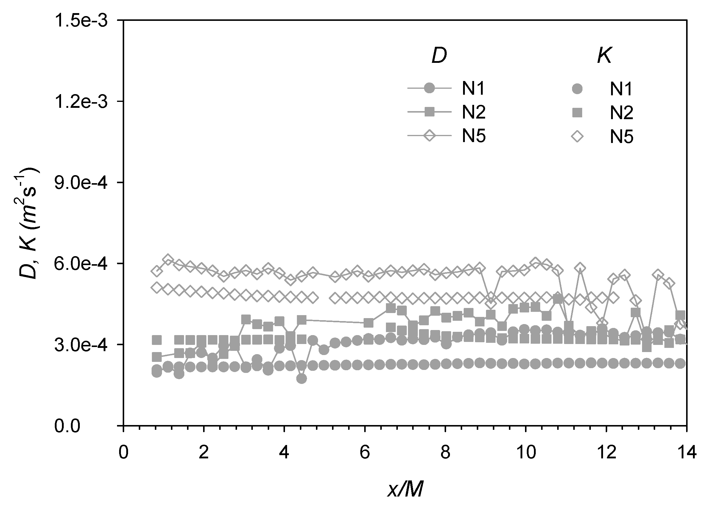
Once the plume development has reached the turbulent-diffusive regime, its spreading rate is dictated by the product of the transverse velocity fluctuation and integral length scale, i.e., the Taylor diffusivity [22], which may therefore be approximated as . As an alternative to the definition above, the Taylor diffusivity may also be estimated from the rate of plume spreading, i.e., the apparent turbulent diffusivity [22], given as
As shown in Figure 10, the Taylor diffusivities D (connected dots) calculated from the velocity data agree reasonably well with the apparent turbulent diffusivity K (unconnected dots) estimated from the plume spreading rate and, hence, the concentration data. Strictly speaking, both diffusivities D and K are valid only when the plume spreading width becomes sufficiently larger than the integral length scale (i.e., when plume development has transitioned from turbulent-convective to turbulent-diffusive). This would translate to a change of slope in the plume spreading width with downstream distance, which is somewhat discernible at x/M = ~4 for cases N1 and N5 in Figure 4b.
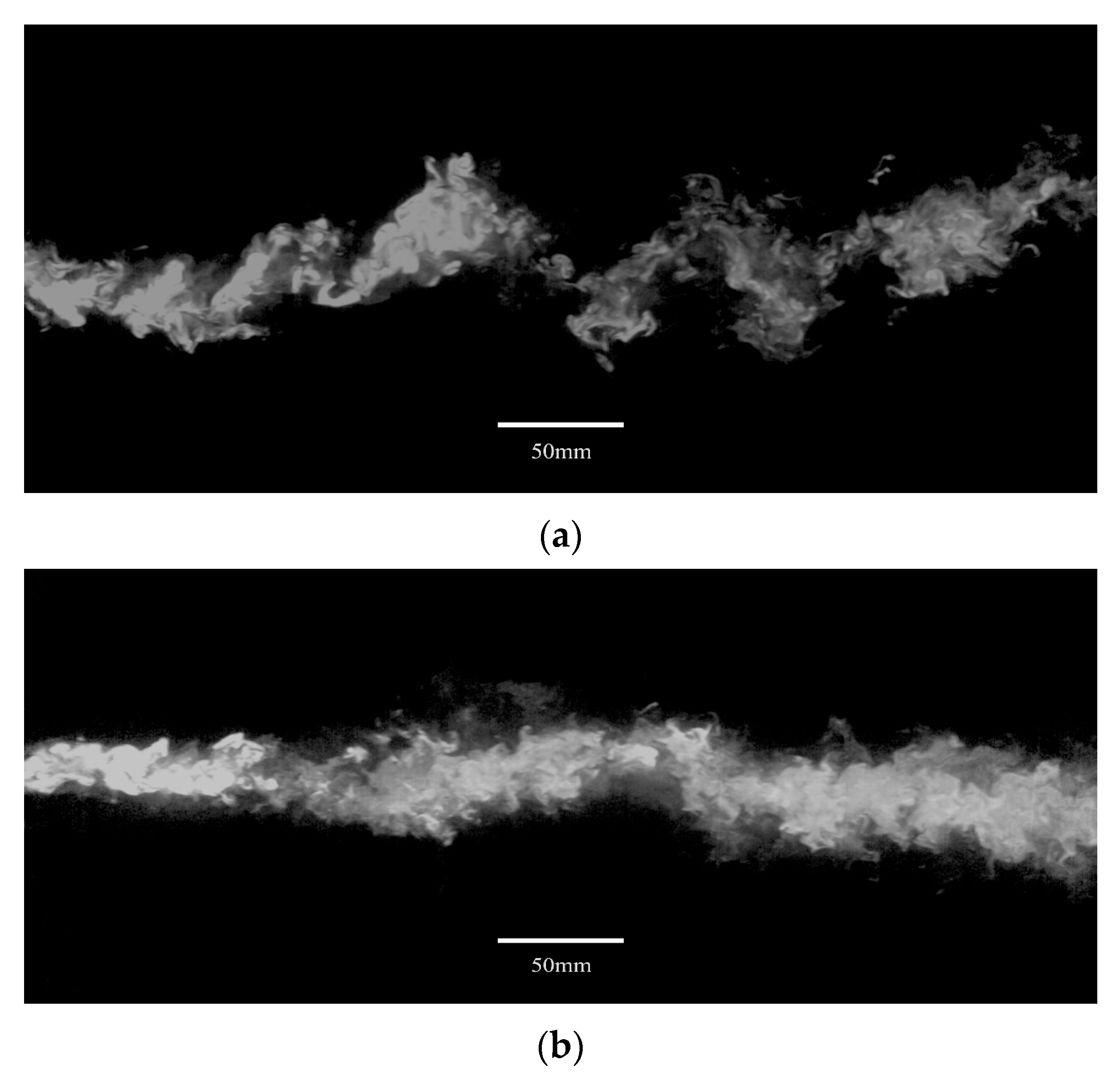
Instantaneous PLIF images (examples shown in Figure 11) suggest that, without the net panel, large coherent eddies were observed to develop and oscillate in the horizontal plane (Figure 11a). However, in the presence of net panel (shown for test case N5), these large eddies were broken into numerous small eddies. The horizontal lateral oscillatory motion of the plume was also significantly weakened (Figure 11b), which was confirmed by the reduced transverse integral length scale for case N5 relative to N0, and the plume spreading width was closer to the integral length scale behind the twine than at the mesh hole (Figure 9). Acting alongside the difference in plume spreading mechanism, i.e., turbulent-convective versus turbulent-diffusive, the resultant spreading widths did not differ significantly (Figure 4b).
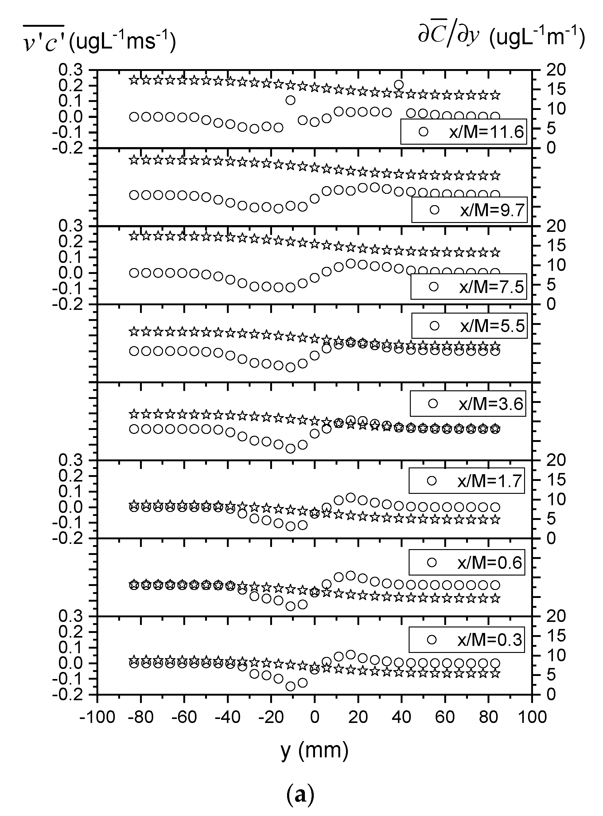
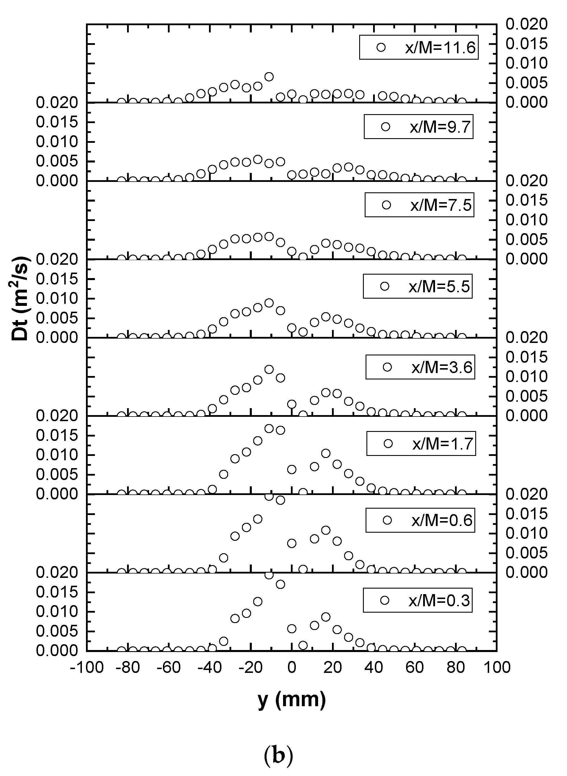
It is also informative to check whether the gradient-diffusion hypothesis that the turbulent scalar flux is proportional to the mean concentration gradient, i.e., , is demonstrated by the current experimental measurements. In this context, Figure 12a plots lateral profiles of the transverse turbulent scalar flux and transverse gradient of mean concentration , showing that their correlation is generally weak. This is also confirmed in Figure 12b by the lateral variability and scatter observed in the turbulent diffusivities D calculated from the ratio of the two quantities and . However, the diffusivity D is shown to become more uniform across the section with increasing downstream distance x/M, and the value at the furthest downstream location (i.e., x/M = 11.6) is also closer to the Taylor diffusivity calculated above (i.e., O(10−4), see Figure 10). These results are generally consistent with previous findings that the gradient-diffusion hypothesis is invalid in the near field region of scalar transport in grid-generated turbulence, where the turbulent flow is still subject to significant anisotropy and inhomogeneity and the plume development has not yet reached the turbulent-diffusive regime [20,32].
4. Conclusions
A combined PIV-PLIF technique was employed in this study to investigate experimentally the wake characteristics and near-field mass transport through fishing net panel positioned vertically and perpendicular to a steady current generated along a water flume channel. The main findings of the study are summarized as follows:
- The wake flow downstream of the model fishing net panel showed a marked reduction and increase in time-averaged streamwise velocity immediately behind the net twine and at the adjacent mesh holes, respectively. The opposite trend was found for the streamwise turbulence intensity. For x > ~3M, the flow field became more homogeneous and entered the turbulence decay region. However, complete recovery of incoming velocity and development of isotropic turbulence was not observed to occur within the downstream extent of experimental measurements (i.e., x → ~15M). Corroborating with these changes in the turbulent flow field, the mean concentration began to decay steadily after x = ~3M.
- Similar to decaying grid-generated turbulence, the turbulence intensity followed a power-law decay over a short range of x = ~4M to 10M. However, the fitted decay exponent was much smaller than reported values for grid turbulence in previous wind-tunnel and water-channel experimental studies. Lateral profiles of the mean scalar concentration and concentration fluctuation exhibited self-similar Gaussian distributions, while those for the transverse turbulent scalar flux were nearly self-similar and antisymmetric about the centerline. These profiles started from a downstream location x = 0.3M, which was much closer to the net panel, with a strongly inhomogeneous wake flow field, than previous findings on scalar plume development downstream of point sources in grid turbulence.
- The presence of the net panel tended to break larger coherent eddies into smaller vortices, leading to a reduction in the transverse integral length scale. In so doing, the panel also accelerated the transition of plume development from the turbulent-convective regime to the more effective turbulent-diffusive regime, with the combined effects leading to slightly enhanced lateral spreading of the scalar plume.
- Direct comparison of the plume spreading width and the transverse integral length scale of the flow indicated that the development of the scalar plume was still transitioning from turbulent-convective regime to turbulent-diffusive regime within the downstream extent of the experimental measurements. This was confirmed by the invalidity of the gradient-diffusion hypothesis in predicting the transverse scalar transport. Nevertheless, the apparent turbulent diffusivity, estimated from the gross plume parameters (i.e., time-averaged velocity and spreading width), appeared to be in reasonable agreement with the Taylor diffusivity calculated as the product of the transverse velocity fluctuation and integral length scale.
In summary, the present laboratory-based study provides novel firsthand experimental data (e.g., simultaneous measurements of planar velocity and concentration fields), as well as useful insights (e.g., flow turbulence characteristics and mass transport), in the near-wake region of a model aquaculture cage net panel. This can clearly help inform future cage-scale field studies and provide a basis for the development of near-field models to assess environmental impact and regulation compliance in cage-based aquaculture. In particular, the improved understanding of the near-field characteristics will help modelers undertaking large-scale numerical modelling to specify appropriate cage-edge boundary conditions, taking full account of near-field hydrodynamic processes and cage design in order to enhance current capability in environmental impact assessment and the optimization of the cage deployment in fish farms.
A particular application of the current research is in assessing the potential benefits of employing “buffer” net panels at the ends of an aquaculture cage array with the aim of reducing hydrodynamic loading on aquaculture cage array, for example, in strongly tidal sites and exposed coastal locations subject to significant wave loading. Prototype field-scale testing of a buffer net panel was recently conducted at an existing fish farm in a strongly tidal sea loch in the northwest of Scotland. Current data collected by Acoustic Doppler Current Profiler (ADCP) deployed at the site clearly suggest that the presence of the buffer net acts to reduce significantly the ebb tidal currents on the lee side of the buffer net panel. However, the clear impact that the placement of buffer net panels adjacent to fish cage arrays has on the hydrodynamics and, hence, the hydrodynamic loading on cage arrays and potentially the mass transport processes from fish cages, clearly warrants further investigation.
The major differences of the results from the present study using fishing net panels, compared to analogous studies of grid-generated turbulence, can be attributed to the geometric and structural net properties (e.g., rigidity, solidity, etc.) and the location of the plume source (i.e., distance upstream or downstream from the nets panel or grid), among other factors. More dedicated experimental studies are needed to verify the effects of the various factors and quantify their influence on near-wake flow behavior and mass transport in the future.
Author Contributions
Conceptualization, D.S. and R.-Q.W.; methodology, L.H.; investigation, L.H.; resources, D.S.; data curation, L.H.; writing—original draft preparation, D.S.; writing—review and editing, R.-Q.W., C.G. & A.C.; visualization, L.H.; supervision, D.S., R.-Q.W., C.G.; project administration, D.S.; funding acquisition, D.S., R.-Q.W., A.C. All authors have read and agreed to the published version of the manuscript.
Funding
This work was supported by the National Natural Science Foundation of China (Grant No. 51779012 and 51811530316), National Key Research and Development Program of China (Grant No. 2018YFC1406404) and Interdisciplinary Research Funds of Beijing Normal University. The authors (DS, RQW and AC) are also grateful for financial support provided by The Royal Society through an International Exchange Cost Share (China) 2017 Grant (Grant No. IEC\NSFC\170104) that facilitated bilateral research visits between Beijing Normal University and the University of Dundee. Financial support for C. Gualtieri from the State Administration of Foreign Experts Affairs of China (Grant No. GDW20181100033) is also grateful acknowledged.
Institutional Review Board Statement
Not applicable.
Informed Consent Statement
Not applicable.
Data Availability Statement
All data necessary to carry out the work in this paper are included in the figures, tables or are available in the cited references.
Conflicts of Interest
The authors declare no conflict of interest.
Nomenclature
| a | constant associated with the power law turbulence decay |
| mean concentration (µg/L) | |
| mean concentration at the plume centerline (µg/L) | |
| mean concentration at the net panels (µg/L) | |
| c’ | concentration fluctuation (µg/L) |
| d | diameter of the net twine (mm) |
| D | Taylor (turbulent) diffusivity (m2/s) |
| ey | transverse unit vector |
| h | water depth in the flume (m) |
| K | apparent turbulent diffusivity (m2/s) |
| Lt | integral length scale of transverse velocity fluctuations (mm) |
| M | mesh size of the net/grid (mm) |
| n | decay rate (exponent) of the power law turbulence decay |
| r | separation in the transverse direction |
| Red | Reynolds number with respect to water depth (=U0 h/ν) |
| Rem | Reynolds number with respect to net twine (=U0 d/ν) |
| Rew | Reynolds number with respect to mesh size (=U0M/ν) |
| S | net solidity defined as the ratio between the projected area and the total area enclosed by the net panel () |
| mean streamwise velocity behind the net (m/s) | |
| U0 | incoming current velocity in the flume (m/s) |
| u’ | velocity fluctuation in the streamwise direction (m/s) |
| v’ | velocity fluctuation in the transverse direction (m/s) |
| transverse turbulent mass flux (µg/L⋅m/s) | |
| x,y,z | Cartesian coordinates in the longitudinal, transverse and vertical directions, respectively (mm) |
| x0 | virtual origin associated with the power law turbulence decay (mm) |
| spreading width of the scalar plume (mm) | |
| spreading with of the concentration fluctuations (mm) | |
| normalized transverse coordinate ( |
References
- Dudley, R.W.; Panchang, V.G.; Newell, C.R. Application of a comprehensive modeling strategy for the management of net-pen aquaculture waste transport. Aquaculture 2000, 187, 319–349. [Google Scholar] [CrossRef]
- Corner, R.A.; Davies, P.A.; Cuthbertson, A.J.S.; Telfer, T.C. A flume study to evaluate the processes governing retention of sea lice therapeutants using skirts in the treatment of sea lice infestation. Aquaculture 2011, 319, 459–465. [Google Scholar] [CrossRef]
- Buryniuk, M.; Petrell, R.J.; Baldwin, S.; Lo, K.V. Accumulation and natural disintegration of solid wastes caught on a screen suspended below a fish farm cage. Aquac. Eng. 2006, 35, 78–90. [Google Scholar] [CrossRef]
- Klebert, P.; Lader, P.; Gansel, L.; Oppedal, F. Hydrodynamic interactions on net panel and aquaculture fish cages: A review. Ocean Eng. 2013, 58, 260–274. [Google Scholar] [CrossRef]
- Price, C.; Black, K.D.; Hargrave, B.T.; Morris, J.A. Marine cage culture and the environment: Effects on water quality and primary production. Aquac. Environ. Interact. 2015, 6, 151–174. [Google Scholar] [CrossRef] [Green Version]
- Laws, E.M.; Livesey, J.L. Flow through Screens. Annu. Rev. Fluid Mech. 1978, 10, 247–266. [Google Scholar] [CrossRef]
- Katopodis, C.; Ead, S.A.; Standen, G.; Rajaratnam, N. Structure of flow upstream of vertical angled screens in open channels. J. Hydraul. Eng. 2005, 131, 294–304. [Google Scholar] [CrossRef]
- Teitel, M.; Dvorkin, D.; Haim, Y.; Tanny, J.; Seginer, I. Comparison of measured and simulated flow through screens: Effects of screen inclination and porosity. Biosyst. Eng. 2009, 104, 404–416. [Google Scholar] [CrossRef]
- Bi, C.W.; Zhao, Y.P.; Dong, G.H.; Xu, T.J.; Gui, F.K. Experimental investigation of the reduction in flow velocity downstream from a fishing net. Aquac. Eng. 2013, 57, 71–81. [Google Scholar] [CrossRef]
- Batchelor, G.K. The Theory of Homogeneous Turbulence; University Press: Cambridge, UK, 1953; 197p. [Google Scholar]
- Mohamed, M.S.; Larue, J.C. The Decay Power Law in Grid-Generated Turbulence. J. Fluid Mech. 1990, 219, 195–214. [Google Scholar] [CrossRef]
- Comte-bellot, G.; Corrsin, S. Use of a Contraction to Improve Isotropy of Grid-Generated Turbulence. J. Fluid Mech. 1966, 25, 657–682. [Google Scholar] [CrossRef]
- Isaza, J.C.; Salazar, R.; Warhaft, Z. On grid-generated turbulence in the near- and far field regions. J. Fluid Mech. 2014, 753, 402–426. [Google Scholar] [CrossRef]
- Cardesa, J.I.; Nickels, T.B.; Dawson, J.R. 2D PIV measurements in the near field of grid turbulence using stitched fields from multiple cameras. Exp. Fluids 2012, 52, 1611–1627. [Google Scholar] [CrossRef]
- Gan, L.; Krogstad, P.A. Evolution of turbulence and in-plane vortices in the near field flow behind multi-scale planar grids. Phys. Fluids 2016, 28. [Google Scholar] [CrossRef] [Green Version]
- Hopfinger, E.J.; Toly, J.A. Spatially Decaying Turbulence and Its Relation to Mixing across Density Interfaces. J. Fluid Mech. 1976, 78, 155–175. [Google Scholar] [CrossRef]
- Desilva, I.P.D.; Fernando, H.J.S. Oscillating Grids as a Source of Nearly Isotropic Turbulence. Phys. Fluids 1994, 6, 2455–2464. [Google Scholar] [CrossRef]
- Cuthbertson, A.J.S.; Dong, P.; Davies, P.A. Non-equilibrium flocculation characteristics of fine-grained sediments in grid-generated turbulent flow. Coast. Eng. 2010, 57, 447–460. [Google Scholar] [CrossRef]
- Nakamura, I.; Sakai, Y.; Miyata, M. Diffusion of matter by a non-buoyant plume in grid-generated turbulence. J. Fluid Mech. 1987, 178, 379–403. [Google Scholar] [CrossRef]
- Lemoine, F.; Antoine, Y.; Wolff, M.; Lebouche, M. Mass transfer properties in a grid generated turbulent flow: Some experimental investigations about the concept of turbulent diffusivity. Int. J. Heat Mass Transf. 1998, 41, 2287–2295. [Google Scholar] [CrossRef]
- Cuthbertson, A.J.S.; Malcangio, D.; Davies, P.A.; Mossa, M. The influence of a localised region of turbulence on the structural development of a turbulent, round, buoyant jet. Fluid Dyn. Res. 2006, 38, 683–698. [Google Scholar] [CrossRef]
- Nedic, J.; Tavoularis, S. Measurements of passive scalar diffusion downstream of regular and fractal grids. J. Fluid Mech. 2016, 800, 358–386. [Google Scholar] [CrossRef]
- Taylor, G.I. Diffusion by continuous movements. Proc. Lond. Math. Soc. 1922, 20, 196–212. [Google Scholar] [CrossRef]
- Lader, P.; Jensen, A.; Sveen, J.K.; Fredheim, A.; Enerhaug, B.; Fredriksson, D. Experimental investigation of wave forces on net structures. Appl. Ocean Res. 2007, 29, 112–127. [Google Scholar] [CrossRef]
- Zhan, J.M.; Jia, X.P.; Li, Y.S.; Sun, M.G.; Guo, G.X.; Hu, Y.Z. Analytical and experimental investigation of drag on nets of fish cages. Aquac. Eng. 2006, 35, 91–101. [Google Scholar] [CrossRef]
- Patursson, O.; Swift, M.R.; Tsukrov, I.; Simonsen, K.; Baldwin, K.; Fredriksson, D.W.; Celikkol, B. Development of a porous media model with application to flow through and around a net panel. Ocean Eng. 2010, 37, 314–324. [Google Scholar] [CrossRef]
- Løland, G. Current forces on, and water flow through and around, floating fish farms. Aquac. Int. 1993, 1, 72–89. [Google Scholar] [CrossRef]
- Lemoine, F.; Antoine, Y.; Wolff, M.; Lebouche, M. Some experimental investigations on the concentration variance and its dissipation rate in a grid generated turbulent flow. Int. J. Heat Mass Transf. 2000, 43, 1187–1199. [Google Scholar] [CrossRef]
- Lemoine, F.; Wolff, M.; Lebouché, M. Experimental investigation of mass transfer in a grid-generated turbulent flow using combined optical methods. Int. J. Heat Mass Transf. 1997, 40, 3255–3266. [Google Scholar] [CrossRef]
- Ito, Y.; Watanabe, T.; Nagata, K.; Sakai, Y. Turbulent mixing of a passive scalar in grid turbulence. Phys. Scr. Int. J. Exp. Theor. Phys. 2016, 91, 074002. [Google Scholar] [CrossRef]
- Warhaft, Z. The interference of thermal fields from line sources in grid turbulence. J. Fluid Mech. 1984, 144, 363–387. [Google Scholar] [CrossRef]
- Li, J.D.; Bilger, R.W. The diffusion of conserved and reactive scalars behind line sources in homogeneous turbulence. J. Fluid Mech. 2006, 318, 339–372. [Google Scholar] [CrossRef]
Figure 1.
Schematic of experimental setup.

Figure 2.
Time-averaged (a) velocity field and (b) concentration field downstream of net for the representative case N5.
Figure 2.
Time-averaged (a) velocity field and (b) concentration field downstream of net for the representative case N5.

Figure 3.
(a) Lateral profiles of normalized velocity at different downstream locations for N5; (b) Variation of with longitudinal distance along flume centerline.
Figure 3.
(a) Lateral profiles of normalized velocity at different downstream locations for N5; (b) Variation of with longitudinal distance along flume centerline.

Figure 4.
(a) Lateral profiles of the normalized time-averaged concentration at different downstream locations for N5; (b) Evolution of the plume spreading width with downstream distance.
Figure 4.
(a) Lateral profiles of the normalized time-averaged concentration at different downstream locations for N5; (b) Evolution of the plume spreading width with downstream distance.


Figure 5.
Longitudinal profiles of the normalized time-averaged concentration along the plume centerline.
Figure 5.
Longitudinal profiles of the normalized time-averaged concentration along the plume centerline.

Figure 6.
(a) Longitudinal evolution of streamwise turbulence intensity behind the central twine and the adjacent mesh hole for case N5; (b) Power decay region of behind the twine for N1 and N5; (c) Lateral profiles of at different downstream locations for N5; (d) Longitudinal profile of the turbulence anisotropy ratio behind the twine and mesh hole for N5.


Figure 7.
(a) Lateral profiles of the root mean square (RMS) of the normalized concentration fluctuation ; (b) Longitudinal evolution of and along the plume centerline.
Figure 7.
(a) Lateral profiles of the root mean square (RMS) of the normalized concentration fluctuation ; (b) Longitudinal evolution of and along the plume centerline.

Figure 8.
Lateral profiles of the normalized transverse turbulent flux .

Figure 9.
Longitudinal development of the transverse turbulent integral length scale for N5.

Figure 10.
Longitudinal profiles of turbulent diffusivities ( and ).

Figure 11.
Instantaneous PLIF images of (a) case N0 without net; (b) case N5 with net.

Figure 12.
Lateral profiles of (a) transverse turbulent scalar flux d transverse gradient of mean concentration an ; (b) turbulent diffusivity .
Figure 12.
Lateral profiles of (a) transverse turbulent scalar flux d transverse gradient of mean concentration an ; (b) turbulent diffusivity .


Table 1.
Experimental parameters.
| No. | Current Velocity U0 (m/s) | Twine Diameter d (mm) | Mesh Size M (mm) | Net Solidity S (%) | Reynolds Number w.r.t. Water Depth Rew = U0h/ν | Reynolds Number w.r.t. Net Twine Red = U0d/ν | Reynolds Number w.r.t. Mesh Size Rem = U0M/ν |
|---|---|---|---|---|---|---|---|
| N0 | 0.290 | / | / | / | 87,000 | / | / |
| N1 | 0.142 | 2 | 20 | 19.0 | 42,600 | 284 | 2840 |
| N2 | 0.290 | 2 | 20 | 19.0 | 87,000 | 580 | 5800 |
| N5 | 0.290 | 1 | 20 | 9.8 | 87,000 | 290 | 5800 |
Table 2.
Comparison of the fitted parameters of the power decay range of streamwise turbulence intensity.
Table 2.
Comparison of the fitted parameters of the power decay range of streamwise turbulence intensity.
| References | Experimental Conditions | Decay Rate n (n with x0 = 0) | Constant a (a with x0 = 0) |
|---|---|---|---|
| Nakamura et al. (1987) [19] | Water channel Regular biplane grids S = 36% ReM = 1480–2970 | 1.45 | 0.0566 |
| Isaza et al. (2014) [13] | Wind tunnel Regular biplane grids S = 34% ReM = 42,000 | (1.90) | (0.489) |
| Nedic and Tavoularis (2016) [22] | Wind tunnel Steel regular grids S = 25% ReM = 51,000–102,000 | 2.34–2.87 (1.82–1.93) | |
| Present study | Water flume Polyethylene knotless square nets S = 9.8–19.0% ReM = 2840–5800 | 0.67–0.85 (0.43–0.55) | 0.023–0.047 (0.011–0.018) |
Publisher’s Note: MDPI stays neutral with regard to jurisdictional claims in published maps and institutional affiliations. |
© 2021 by the authors. Licensee MDPI, Basel, Switzerland. This article is an open access article distributed under the terms and conditions of the Creative Commons Attribution (CC BY) license (http://creativecommons.org/licenses/by/4.0/).
Share and Cite
MDPI and ACS Style
Shao, D.; Huang, L.; Wang, R.-Q.; Gualtieri, C.; Cuthbertson, A. Flow Turbulence Characteristics and Mass Transport in the Near-Wake Region of an Aquaculture Cage Net Panel. Water 2021, 13, 294. https://doi.org/10.3390/w13030294
AMA Style
Shao D, Huang L, Wang R-Q, Gualtieri C, Cuthbertson A. Flow Turbulence Characteristics and Mass Transport in the Near-Wake Region of an Aquaculture Cage Net Panel. Water. 2021; 13(3):294. https://doi.org/10.3390/w13030294
Chicago/Turabian StyleShao, Dongdong, Li Huang, Ruo-Qian Wang, Carlo Gualtieri, and Alan Cuthbertson. 2021. "Flow Turbulence Characteristics and Mass Transport in the Near-Wake Region of an Aquaculture Cage Net Panel" Water 13, no. 3: 294. https://doi.org/10.3390/w13030294
Note that from the first issue of 2016, this journal uses article numbers instead of page numbers. See further details here.