An RF-PCE Hybrid Surrogate Model for Sensitivity Analysis of Dams

Abstract

Quantification of structural vibration characteristics is an essential task prior to perform any dynamic health monitoring and system identification. Anatomy of vibration in concrete arch dams (especially tall dams with un-symmetry shape) is very complicated and requires special techniques to solve the eigenvalue problem. The situation becomes even more complicated if the material distribution is assumed to be heterogeneous within the dam body (as opposed to conventional isotropic homogeneous relationship). This paper proposes a hybrid Random Field (RF)–Polynomial Chaos Expansion (PCE) surrogate model for uncertainty quantification and sensitivity assessment of dams. For different vibration modes, the most sensitive spatial locations within dam body are identified using both Sobol’s indices and correlation rank methods. Results of the proposed hybrid model is further validated using the classical random forest regression method. The outcome of this study can improve the results of system identification and dynamic analysis by properly determining the vibration characteristics.

1. Introduction

Determination of the vibration characteristics in concrete dams (especially the unsymmetrical tall arch dams) is an essential task prior to perform any nonlinear seismic analysis [1], dynamic health monitoring [2,3], and system identification [4,5]. This research topic has received a lot of recognition in the past few years [6] and several advanced techniques have been developed such the one by Sevieri and De Falco [7] based on Bayesian interface model. Among many assumptions to formulate the numerical model, the most fundamental one is isotropic homogeneous concrete (or at least zoned concrete) material distribution within the dam body [8]. While this assumption can be valid for new dams or those without (visible or hidden) physical damage, it cannot be used widely for damaged or aged dams. In fact, several recent research shows that macro-scale heterogeneity [9] might have a great influence on the dynamic characteristics of large concrete structures (i.e., concrete dams [10] and nuclear containment buildings [11]).

The main objective in this paper is to solve the heterogeneous vibration analysis and dynamic identification of arch dams using surrogate modeling. Polynomial chaos expansion (PCE) is used in conjunction with Latin Hypercube sampling (LHS) and random fields (RF) theory. The hybrid RF-PCE surrogate model is then used to identify the most sensitive regions of two (symmetry and un-symmetry) arch dams at different vibration modes. Such a hybrid meta-model has not been used before for dams in any level. The findings of this study will help to identify the locations of dams (and any other infra-structure) which most contribute to various vibration frequencies. This will be later used to perform a successful transient analysis for large-scale heterogeneous structures and can greatly improve the model validation and verification.

First, a comprehensive literature review is provided in Section 1.1, followed by a brief review on theory of random fields, polynomial chaos expansion and introducing the hybrid model in Section 2. The case study dams are explained in Section 3, and the results are discussed in Section 4. Finally, the PCE-based sensitivity analysis is validated by classical random forest method in Section 5.

Literature Review

This section provides a literature review on the application of PCE meta-model for dams and some other infra-structures.

Guo et al. [12] investigated the reliability analysis of an embankment dam by sparse PCE, as well as identification of the most important random variables (RVs) by Sobol indices. Two different deterministic approaches were compared to probabilistic method. The results showed that deterministic approaches lead to similar reliability results in terms of the failure probability, $P_f$, distribution of the first order second moment (FOSM), and sensitivity index for each RV. They reported that soil dry density, effective cohesion, and friction angle have the most dominant effect on the sliding stability assessment of the embankment dam. Sevieri et al. [13] proposed a framework for post-earthquake safety assessment of the existing dams. The Bayesian updating technique was applied to reduce the uncertainties related to modeling procedure, material properties and geometry definition of gravity dams. The finite element (FE) model response related to water level variation was approximated via PCE method, and used for calibration. Hariri-Ardebili and Sudret [14] investigated the application of PCE meta-model in uncertainty quantification (UQ) of different implicit and explicit dam engineering problems. They found that PCE can develop a surrogate model with a very limited number of initial simulations and reduce the computational time considerably. Even the sample size as low as 5% of the initial database can provide an acceptable engineering result. They performed a comprehensive parametric study on the impact of different sample sizes, quantity of interests (QoIs), statistical parameters (e.g., mean, variance, error), sampling methods (e.g., LHS, Halton, Sobol), and spatial variability.

Aside from dam engineering problems, the PCE has been practiced in some other engineering fields, too. Kim [15] performed a comparative study on the capability of meta-models in UQ of building energy model. To bypass the inherent high computational cost of building performance simulation tools, PCE method along with Gaussian process emulator (GPE) were applied. The results on total energy consumption of a real case study demonstrated that both meta-models can be used as an alternative to crude Monte Carlo simulation (MCS). They reported that GPE lead to more reliable outputs than PCE on which number of sampling is increased. Wei et al. [16] implemented PCE-based UQ of mechanical properties in dynamic analysis of fiber reinforced polymer (FRP). Longitudinal elastic, transverse elastic, shear, and Young’s modulus were considered as RVs, while the QoIs were assumed to be natural frequencies, modal mass and absolute peak acceleration at the mid mid-span of the bridge. They found the RVs have more impact of natural frequencies compared to modal mass. Slot et al. [17] applied PCE and Kriging meta-models to perform fatigue reliability assessment of a wind turbine with wind direction, wind speed, turbulence, wind shear, air density, and flow inclination as RV. Overall, they reported that Kriging meta-model leads to more accurate results compared to PCE for the studied turbine. Ni et al. [18] performed a PCE-aided UQ of bridge structures including: eigenvalue analysis, dynamic analysis of a linear bridge-vehicle system, and probabilistic nonlinear seismic structural analysis of a bridge. Surrogate-assisted results were compared and contrasted with crude MCS and FOSM approaches. It has been shown that PCE-assisted UQ demonstrates a better performance in terms of accuracy and efficiency. As an application of using meta-models in the context of nuclear engineering, Bouhjiti et al. [19] applied PCE method to develop a global stochastic FE method to predict the uncertainty propagation in a thermo-hydro-mechanical leakage (THM-L) model. It is a framework to simulate the behavior of large reinforced and pre-stressed structures under uncertainties due to material and loading. The PCE-assisted UQ reduces the RVs and facilitates the probabilistic representation of the THM-L model through a cost-effective reliability analysis.

In connection with random fields, Dubreuil et al. [20] developed an adaptive RF representation dedicated to the approximation of extreme value statistics. The proposed approach was based on a discretization of RF by hybrid PCE-Kriging approaches and could provide an accurate presentation of the global extremum for any realization. This framework benefits from partial least square and sparse PCE algorithms in the Kriging and PCE meta-models, respectively. It was concluded that hybrid application of PCE and Kriging methods could play an important role in terms of RF discretization. Guo et al. [21] performed a RF-RV reliability analysis of an earth dam in terms of sliding stability considering the soil uncertainties. Performance assessment of different reliability approaches such as crude MCS, subset simulation (SS), moment method (MM), hybrid sparse PCE-global sensitivity analysis (SPCE/GSA), and coupled sparse PCE-sliced inverse regression (SPCE/SIR), were investigated. Results indicated that the most accurate and efficient methods are SPCE/GSA and SS. In addition, they reported that efficiency of surrogate-aided approaches mainly relies on the number of input RVs. Then, in a SPCE/GSA-based stability study, Guo et al. [22] focused on the effect of cross-correlation dependency between effective cohesion and friction angle considering RF representation of soil parameters via Karhunen-Loève expansion. QoIs were assumed be PDF, model response statistical parameters, failure probability and Sobol index of each RV. It has been concluded that applying spatial variability for embankment dams leads to lower $P_f$ estimation and disperse safety factor values. Furthermore, the $P_f$ is increased with increasing the auto-correlation distance, cross-correlation and coefficient of variation (COV). Mishra et al. [23] proposed a PCE-assisted reliability based life-cycle management framework for buried pipelines under time-variant corrosion damage. After developing the PCE meta-model, an optimization algorithm was proposed to address the life-cycle management of buried pipelines. They concluded that PCE-based RF development facilitates the probabilistic configuration and temporal correlation of corrosion depth.

2. Background Theory

2.1. Polynomial Chaos Expansion

The computational model of an structural system can be represented by $\mathcal{M}$ as a function of M input parameters which are modeled by a M dimensional $\mathit{X}=\left\{X_1,X_2,\dots ,X_M\right\}$, and marginal probability density functions $f_{X_i},i=1,\dots ,M$. The scalar QoI resulted from this system is a RV, denoted $Y=\mathcal{M}\left(\mathit{X}\right)$, and can be represented as a PCE [24] with limited to a finite sum:

$$Y^{PCE}={\mathcal{M}}^{PCE}\left(\mathit{X}\right)=\sum _{\alpha \in \mathcal{A}}{y}_{\alpha }{\mathsf{\Psi }}_{\alpha }\left(\mathit{X}\right),$$

(1)

where ${\mathsf{\Psi }}_{\alpha }\left(\mathit{X}\right)$ are the multi-variate polynomials orthonormal with respect to $f_{\mathit{X}}$, $y_{\alpha }$ are the expansion coefficients, $\alpha$ are multi-indices that identify the components of the multi-variate polynomials, and $\mathcal{A}$ is the truncation set of multi-indices of cardinality P. This format of PCE is typically used for simulation-based uncertainty quantification problems.

There are two main truncation schemes, i.e., standard [25] and hyperbolic [26]. The hyperbolic truncation is a modification to the standard version (which is based on selection of all polynomials in M input RVs of total degree not exceeding p), and uses the parametric q-norm to define the truncation (for q = 1, the hyperbolic truncation is identical to the standard one):

$${\mathcal{A}}^{M,p,q}=\left\{\mathbf{\alpha }\in {\mathcal{A}}^{M,p}:{∥\mathbf{\alpha }∥}_q\le p\right\},{∥\mathbf{\alpha }∥}_q={\left(\sum _{i=1}^M{\alpha }_i^q\right)}^{1/q}.$$

(2)

The main objective in PCE framework is to determine the expansion coefficients [14]. In this paper, a non-intrusive approach is adopted which relies on post-processing the outputs resulted from simulation-based methods [27]. According to the least angle regression (LAR), only the polynomials with large impact on the QoIs are retained, while the other are wiped. The LAR method is based on determination of coefficients $\mathbf{y}$ to minimize the mean square error (MSE) including a penalty term of the form $\lambda {∥\mathbf{y}∥}_1$ as discussed by Efron et al. [28]:

$$\widehat{\mathbf{y}}=\underset{\mathbf{y}\in {\mathbb{R}}^P}{\arg \min }\mathbb{E}\left[{\left({\mathbf{y}}^T\mathsf{\Psi }\left(\mathit{X}\right)-\mathcal{M}\left(\mathit{X}\right)\right)}^2\right]+\lambda {∥\mathbf{y}∥}_1,$$

(3)

where ${∥\widehat{\mathbf{y}}∥}_1={\sum }_{\alpha }\left|y_{\alpha }\right|$ is the regularization term that forces the minimization to favor sparse solutions [26].

In the LAR algorithm, first initialize the parameters, $y_{\alpha }=0$; candidate set of ${\mathsf{\Psi }}_{\alpha }$, active set of 0, and set the residuals equal to the vector of observations $\mathbf{y}$. Second, find the vector ${\mathsf{\Psi }}_{{\alpha }_j}$ which is most correlated with the current residual. Move $y_{\alpha }$ from zero towards their least-square value until their regressors ${\mathsf{\Psi }}_{{\alpha }_j}$ are equally correlated to the residual as some other regressor in the candidate set. Next, compute the leave-one-out (LOO) error, $Er{r}_{LOO}^j$ for the current iteration, update all the active coefficients, and move ${\mathsf{\Psi }}_{{\alpha }_j}$ from candidate set to the active set. Finally, continue this step until the size of the active step becomes $min\left(N-1,P\right)$. The LOO cross validation technique is intended to overcome the over-fitting [29] based on the following relationship:

$$Er{r}_{LOO}=\frac{{\sum }_{i=1}^N{\left(\frac{\mathcal{M}\left({\mathbf{x}}^{\left(i\right)}\right)-{\mathcal{M}}^{PCE}\left({\mathbf{x}}^{\left(i\right)}\right)}{1-\mathrm{diag}\left(\mathbf{A}{\left({\mathbf{A}}^T\mathbf{A}\right)}^{-1}{\mathbf{A}}^T\right)}\right)}^2}{{\sum }_{i=1}^N{\left(\mathcal{M}\left({\mathbf{x}}^{\left(i\right)}\right)-\frac{1}{N}{\sum }_{i=1}^N\mathcal{M}\left({\mathbf{x}}^{\left(i\right)}\right)\right)}^2},$$

(4)

where ${\mathbf{A}}_{N\times P}$ is the information matrix, which contains evaluations of all base polynomials at all points of the DOE.

2.2. Random Fields

In structural engineering, the random fields are typically used for characterizing the spatial variability in the material properties or modeling in various micro to macro-level heterogeneity [11]. Different random fields are formulated based on the nature of the uncertainty within the studied stochastic environment [30]. Detailed formulation of the random fields and their validation is beyond this paper and only the fundamental equations are provided (details can be found in Reference [31]). A random field is formulated in a general form of:

$$H\left(\mathbf{x}\right)=\mu \left(\mathbf{x}\right)+\eta \left(\mathbf{x}\right),$$

(5)

where $\mu$, $\eta$, and $\mathbf{x}$ are mean function, random function (with zero mean and an auto-covariance of $C_{aa}$), and position vector, respectively. The auto-covariance function is defined as:

$$C_{aa}(\xi ,{\sigma }_0)={\sigma }_0^2{\rho }_{aa}\left(\xi \right),$$

(6)

where $\xi =\left|\mathbf{x}-{\mathbf{x}}^{\prime }\right|$ is the distance between any two arbitrary points, ${\sigma }_0$ is standard deviation, and ${\rho }_{aa}\left(\xi \right)$ refers to the auto-correlation function, and is defined as:

$${\rho }_{aa}\left(\xi \right)=exp\left(-{\left(\frac{\xi }{l_{corr}}\right)}^2\right),$$

(7)

where $l_{corr}$ is the correlation length.

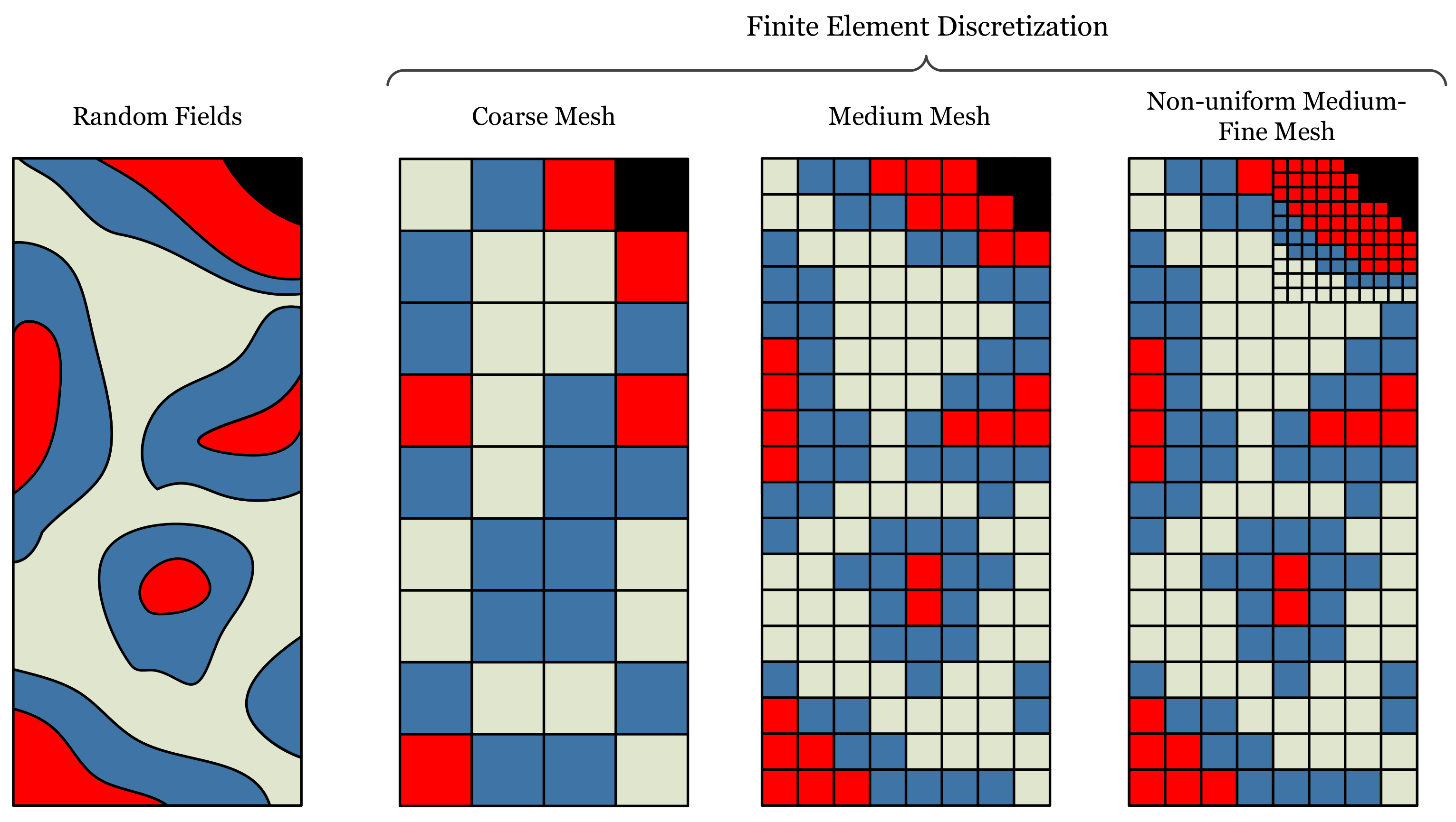
In this paper, the random fields generation is based on covariance matrix decomposition. In addition, a simple midpoint discretization technique [32] is used to transfer the continuous nature of random fields into the finite element mesh. A sample 2D random fields is shown in Figure 1 including its finite element discretization with three types of meshes: coarse, medium, and non-uniform medium-fine. The non-uniform discretization is used in cases where the local response is sensitive to the property distribution in that area (e.g., local fracture). There is a direct relation between the correlation length, $l_{corr}$, and the size of the optimal mesh. The smaller the $l_{corr}$, the finer the mesh should be to properly capture the random fields transition. The number of realizations/samples is typically optimized using the LHS technique [33].

2.3. Lanczos Algorithm for Eigenvalue Problems

Since the hybrid RF-PCE is applied on the frequency response of the coupled system, a brief review is provided for the readers interested in direct implementation. Frequency analysis is performed beginning with a free vibration linear equation of motion and neglecting the damping term as $\mathbf{M}\left\{\ddot{\mathbf{u}}\right\}+\mathbf{K}\left\{\mathbf{u}\right\}=\mathbf{0}$, where $\mathbf{M}$ and $\mathbf{K}$ are global mass and stiffness matrices, and $\left\{\mathbf{u}\right\}$ is the displacement vector. Let us assume a harmonic motion for the displacement, $\mathbf{u}={\left\{\varphi \right\}}_{i}sin\left({\mathbf{\omega }}_{i}t+{\mathbf{\theta }}_i\right)$, where ${\left\{\varphi \right\}}_i$ and ${\mathbf{\omega }}_i^2$ = ${\mathbf{\lambda }}_i$ are eigenvectors and eigenvalues, respectively. Substituting $\mathbf{u}$ into the equation of motion leads to the following non-trivial solution: $det\left(\mathbf{K}-{\mathbf{\lambda }}_i\mathbf{M}\right)=\mathbf{0}$. This is a so-called eigenvalue problem that may be solved for up to n eigenvalues, where n is the number of degrees of freedoms (DOF). The number of unknowns is one more than the number of equations; therefore, an additional equation is needed to solve the problem. Two methods are available to provide such an additional equation, namely: (1) mode shape normalization to mass matrix, ${\left\{\varphi \right\}}_i^T\mathbf{M}{\left\{\varphi \right\}}_i=\mathbf{1}$; and (2) mode shape normalization to unity, where the largest vector component ${\left\{\varphi \right\}}_i$ is set to a value of one.

Many techniques can be used to solve this equation, some of which are listed in Reference [34]. The direct block Lanczos algorithm is a computationally efficient and easy-to-implement technique for solving eigenvalue problems. Originally proposed by Lanczos [35] and based on an extension of the power method, this technique was numerically unstable and wound up being modified by Newman and Ojalvo [36] using a method for purifying vectors in order to stabilize the solution. A detailed theoretical formulation of Lanczos’ algorithm can be found in References [37,38].

Given a square matrix $\mathbf{S}$, the values of ${\left\{\varphi \right\}}_i$ (eigenvector) and ${\mathbf{\lambda }}_i$ (eigenvalues) are of interest in the form of: $\mathbf{S}{\left\{\varphi \right\}}_i={\mathbf{\lambda }}_i{\left\{\mathbf{\varphi }\right\}}_i$. Lanczos’ algorithm provides a tri-diagonal matrix, $\mathbf{T}$, at the end of any step, in which its extreme eigenvalues approximate the extreme eigenvalues of matrix $\mathbf{S}$. To determine these eigenvalues, let us suppose that ${\mathbf{q}}_1$ is a random vector with $\left|{\mathbf{q}}_1\right|=1$. Next, let us compute the $\delta$ and $\beta$ values from Algorithm 1. Then, develop matrix $\mathbf{T}$ and identify the eigenvalues. Being tri-diagonal facilitates the eigen-decomposition of the matrix when using the power method. Note that ${\mathbf{q}}_i$ should be orthogonal to all other $\mathbf{q}$ vectors.

$$\mathbf{T}=\left[\begin{array}{cccccc}{\delta }_1& {\beta }_2& & & & \\ {\beta }_2& {\delta }_2& {\beta }_3& & & \\ & {\beta }_3& \ddots & \ddots & & \\ & & \ddots & \ddots & \ddots & \\ & & & \ddots & {\delta }_{m-1}& {\beta }_m\\ & & & & {\beta }_m& {\delta }_m\end{array}\right].$$

(8)

Algorithm 1: Computation of $\delta$ and $\beta$.

1: ${\mathbf{q}}_0=\mathbf{0}and{\beta }_1=0$ 2: for$i=1,\dots ,m$do 3:     $\mathbf{w}=\mathbf{S}{\mathbf{q}}_i-{\beta }_i$ 4:     ${\mathbf{q}}_{i-1}$ 5:     ${\delta }_i=\mathbf{w}.{\mathbf{q}}_i$ 6:     $\mathbf{w}=\mathbf{w}-{\delta }_i{\mathbf{q}}_i$ 7:     ${\beta }_{i+1}=\left|\mathbf{w}\right|$ 8:     ${\mathbf{q}}_{i+1}=\mathbf{w}/{\beta }_{i+1}$ 9: end for

2.4. Hybrid Method

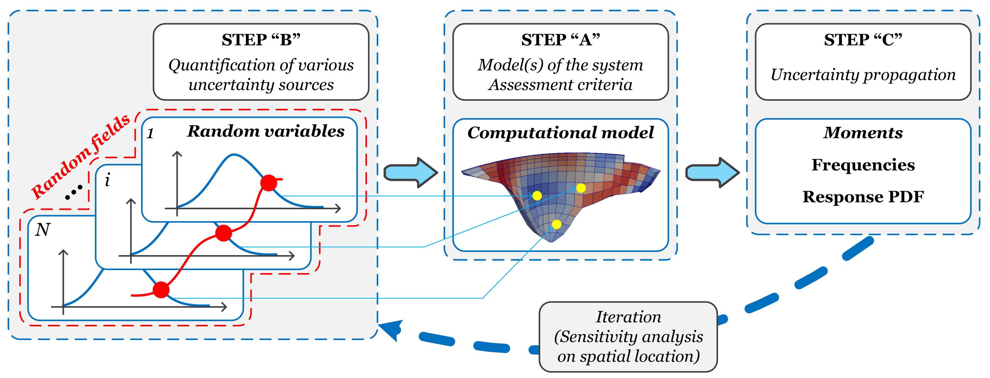
The objective of this paper was to combine the random fields concept with PCE to quantify the uncertainties in the heterogeneous dam models. Moreover, the developed surrogate model will be used for sensitivity analysis of the most important regions within dam body. The initial framework of the uncertainty quantification introduced by Sudret [39] and used by Hariri-Ardebili and Sudret [14] for RV-based assessment of dam structures is expanded in this paper to incorporate the impact of spatial correlation. This framework has three main elements as illustrated in Figure 2:

• Step A: Develop a computational model (i.e., a dam finite element model) which has a role of black-box in the form of $Y=\mathcal{M}\left(\mathit{X}\right)$ (and connects inputs to outputs).
• Step B: Quantify the uncertainty in the input parameters, $\mathit{X}$, either in the form of random variables (correlated or uncorrelated) or random fields.
• Step C: Perform an uncertainty analysis that combines the input uncertainties with the computational model, and quantifies characteristics of the stochastic system. The PCE meta-model, ${\mathcal{M}}^{PCE}$, will be used for this purpose.

The final goal in this paper (as discussed in Section 4) is to answer this important question: “Is it possible to use the PCE-assisted surrogate model for sensitivity and uncertainty quantification of heterogeneous concrete dam models?” Moreover, the findings will be verified by classical random forest method (as discussed in Section 5).

3. Case Study Dams

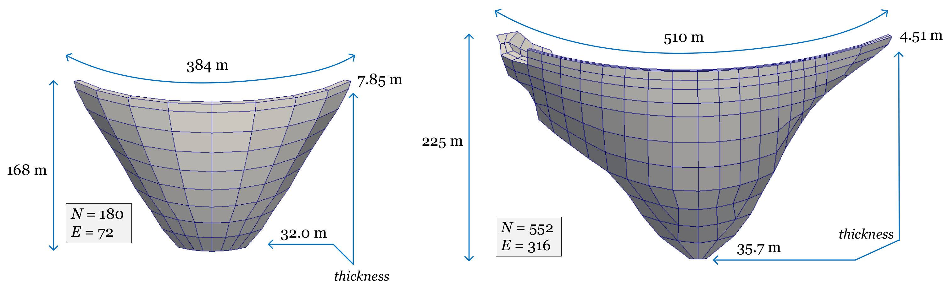
In order to evaluate the capability of PCE in conjunction with random fields in dam engineering problems, two case study dams are studied in this paper. Those two case studies have different number of random variables. Each random variable is indeed a region/element within the dam which reflects the spatial variability of material properties. In both dams, only the concrete modulus of elasticity is assumed to be random variable (due to potential aging and, therefore, reduction of elasticity), while all other material properties are kept in their mean value. One may note that concrete strength is also random (and typically is reduced due to aging); however, it is not used during modal analysis.

In the first one, a coarse mesh is used to reduce the number of input parameters in the PCE meta-model. This symmetry model (hereafter Dam-1) includes only 72 random variables. This example is representative of dams which are constructed with different types of cement (and/or concrete strength) at different locations (typically various concreting regions). Modulus of elasticity, mass density, and Poisson’s ratio of dam body are 25 GPa, 2450 kg/m³, and 0.17, respectively.

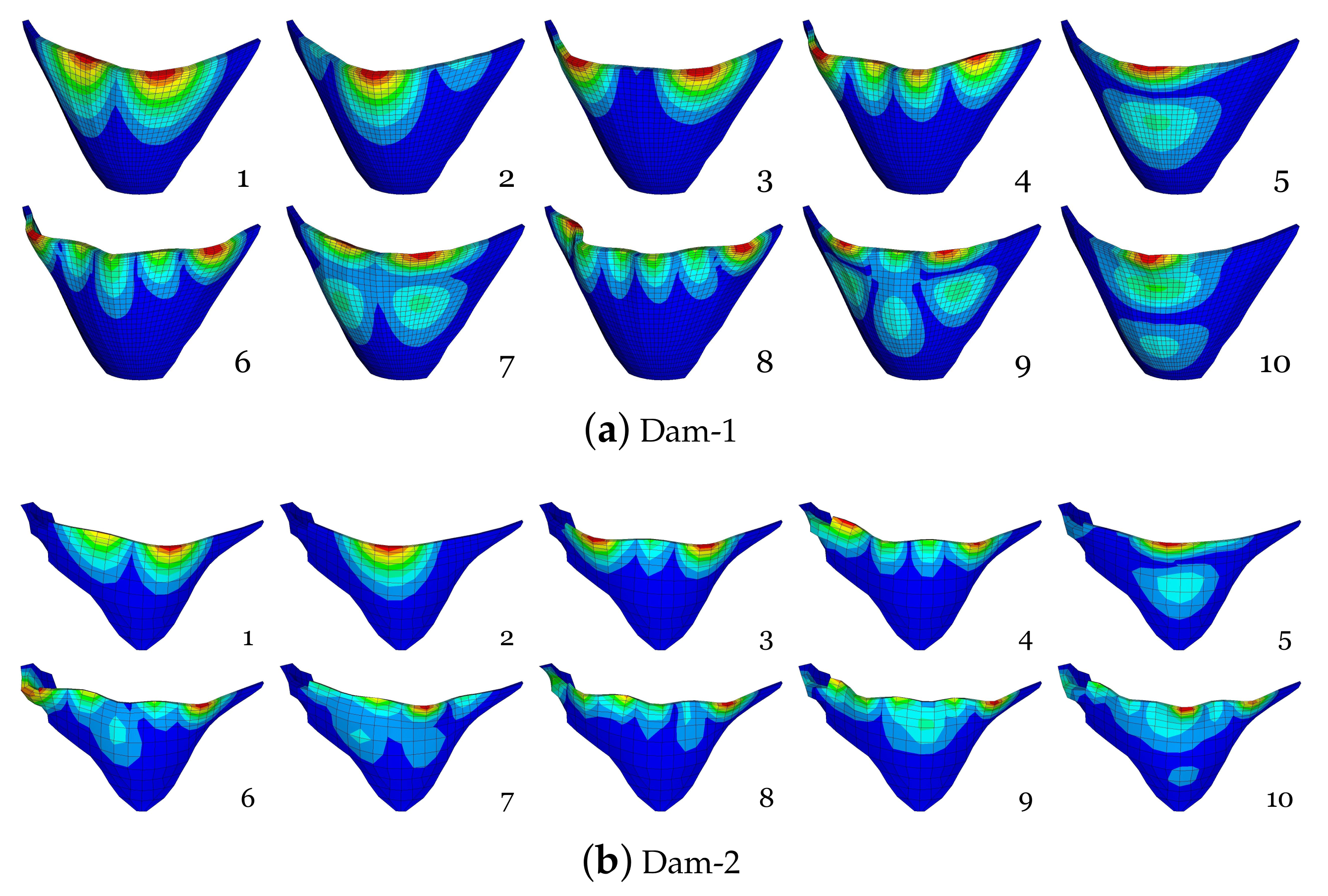
The second example is an un-symmetry dam (hereafter Dam-2) with finer mesh (316 input parameters). This example challenges the capability of the developed meta-model for high-dimensional problems, and can be representative of a dam suffering from non-uniform aging/deterioration. Modulus of elasticity, mass density, and Poisson’s ratio of dam body are 19 GPa, 2450 kg/m³, and 0.18, respectively. Finite element models of the case study dams are illustrated in Figure 3. The slenderness coefficient of Dam-2 is 13.8 compared to 9.9 in Dam-1. Figure A1 illustrates the first ten vibration modes in both dams.

4. Results: Correlation-Based vs. Variance-Based Decomposition

This section will discuss the results of implementation of PCE surrogate model to quantify the sensitivity of the spatial location in arch dams for various vibration modes.

4.1. Dam 1

PCE meta-models are developed based on LAR method. A fixed truncation strategy along with a degree-adaptive sparse PCE option are applied. Hence, q-norms equal to 0.75, and polynomial degrees p set to <2:5>. Three QoIs are evaluated: frequency of vibration, effective mass, and participation factor.

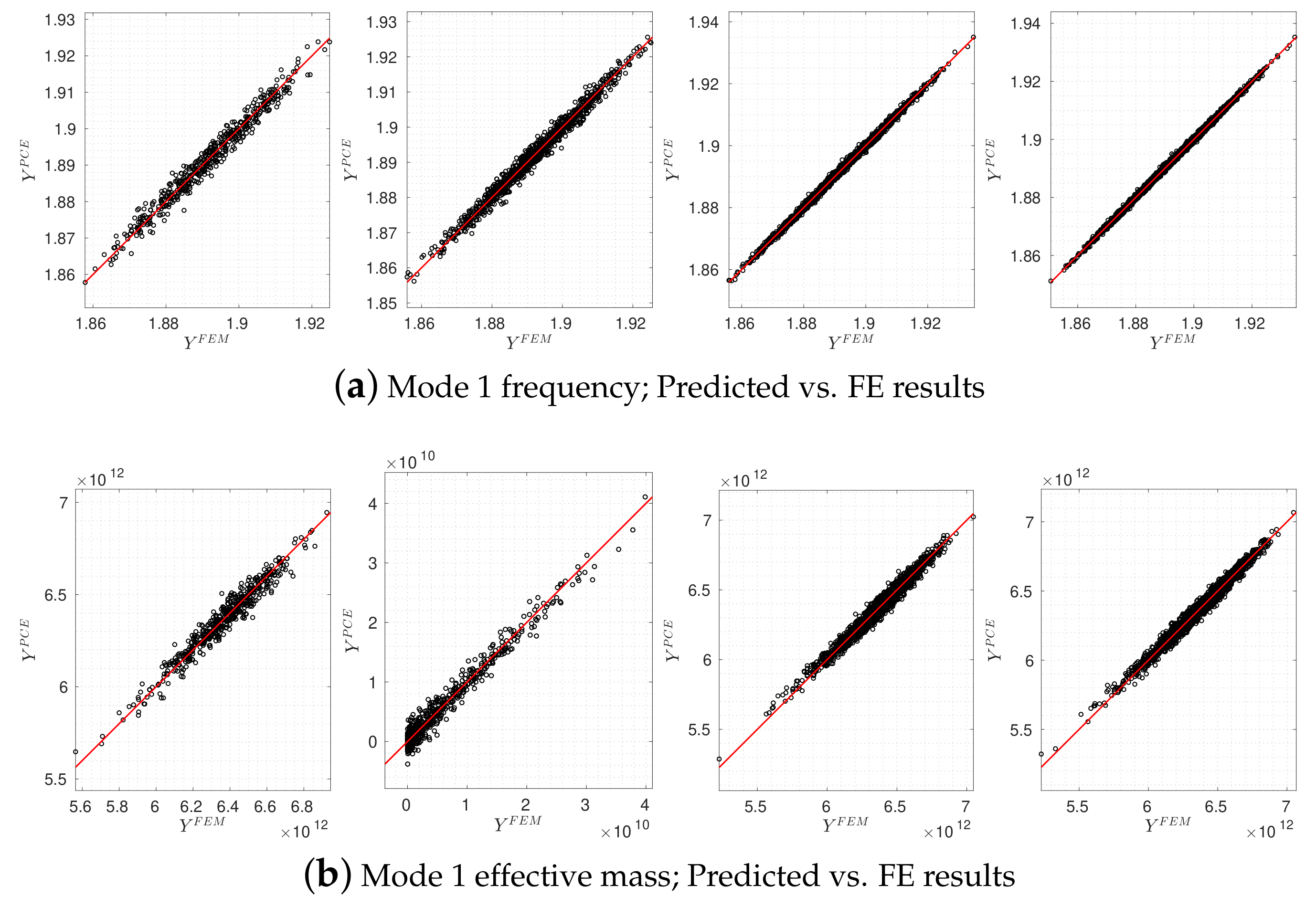
Different DOEs (with 100 to 1000 points) are used to evaluate the sensitivity and accuracy of the prediction. Figure 4 compares the response prediction via PCE and the corresponding expansion coefficients. Five initial (and deterministic) design of experiment (DOE) values are considered, i.e., 100, 200, 400, 800, and 1000. Clearly, increasing the initial sample size, increases the accuracy of PCE meta-model. In addition, it increases the number of expansion coefficients required for the meta-modeling. Qualitatively, the performance of the PCE for frequency response is very similar to the effective mass. The results of participation factor are not shown as they are very similar to other two responses.

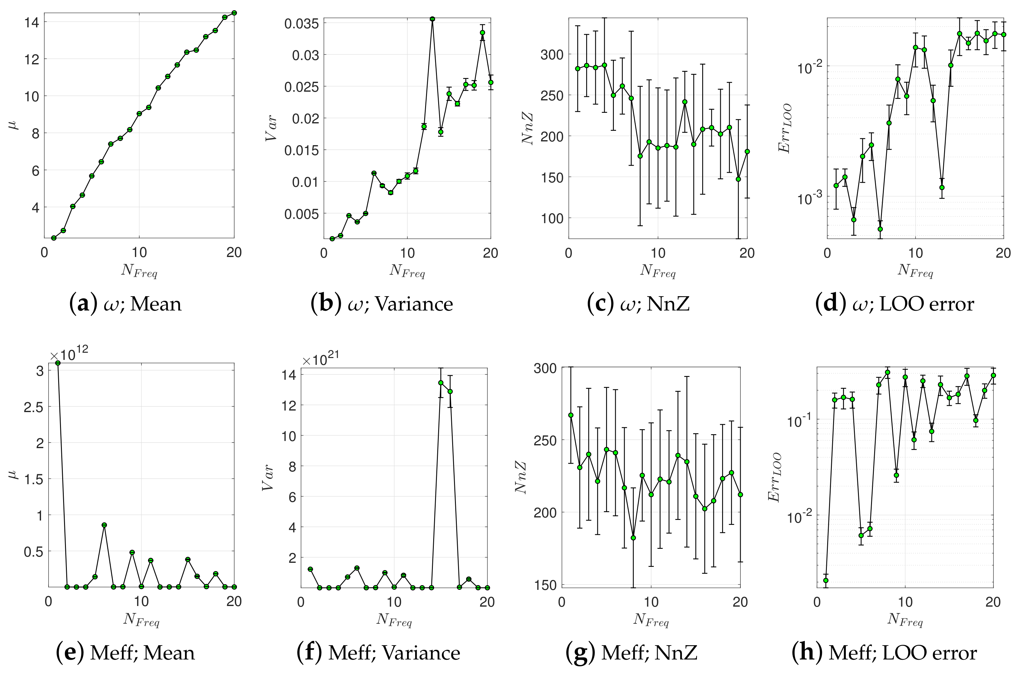
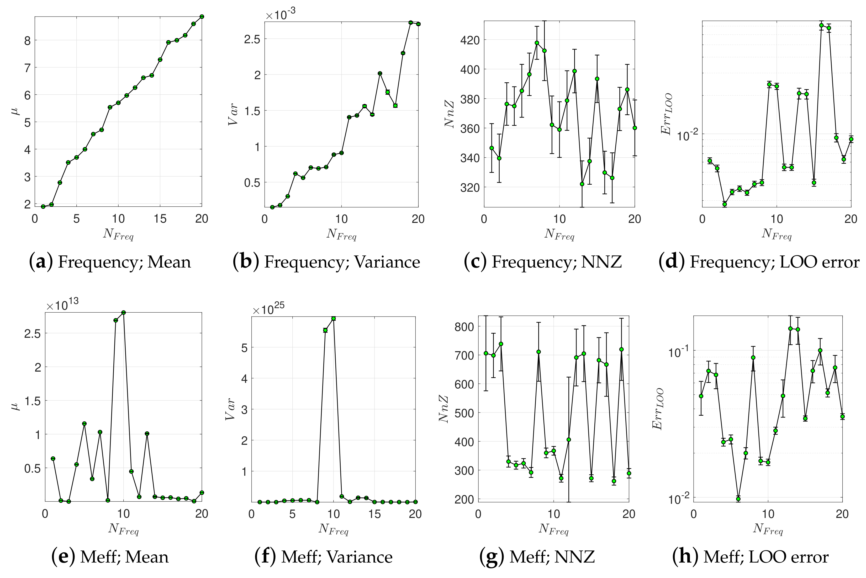
Figure 4 only studied the 1st vibration mode. Next, the effects of higher-modes are evaluated. A batch with 800 initial DOEs is considered to be the pilot Dam-1 model, and the results are expanded for 20 modes. In each case, a similar PCE model as of mode #1 is implemented. To reduce the uncertainties due to initial random selection of DOE points, a total of 20 replications is performed. Therefore, the developed meta-models have a probabilistic nature; see Figure 5.

According to Figure 5a,b the mean and variance increase as a function of frequency. While the mean frequency has a quite uniform form, there are some nonlinear variations for the frequency variance (with some spikes). Based on Figure 5c, the non-zero coefficients is constant for the first 4 modes (and about 280), then it drops to about 180 at mode #8 and keeps a nearly constant trend. There is a considerable probabilistic dispersion in the non-zero (NnZ) value depending on the initial sampling batch. Finally, the LOO error has an increasing trend with some big spikes and small dispersion; see Figure 5d.

As opposed to frequency response, there is not a clear trend for the effective mass in the case of mean and variance response; see Figure 5e,f. Moreover, the NnZ has a fluctuating pattern and from mode #1 to #20 decreases from about 270 to 220; see Figure 5g. The LOO error has an oppose behavior with respect to NnZ and increases with a fluctuating fashion; see Figure 5h.

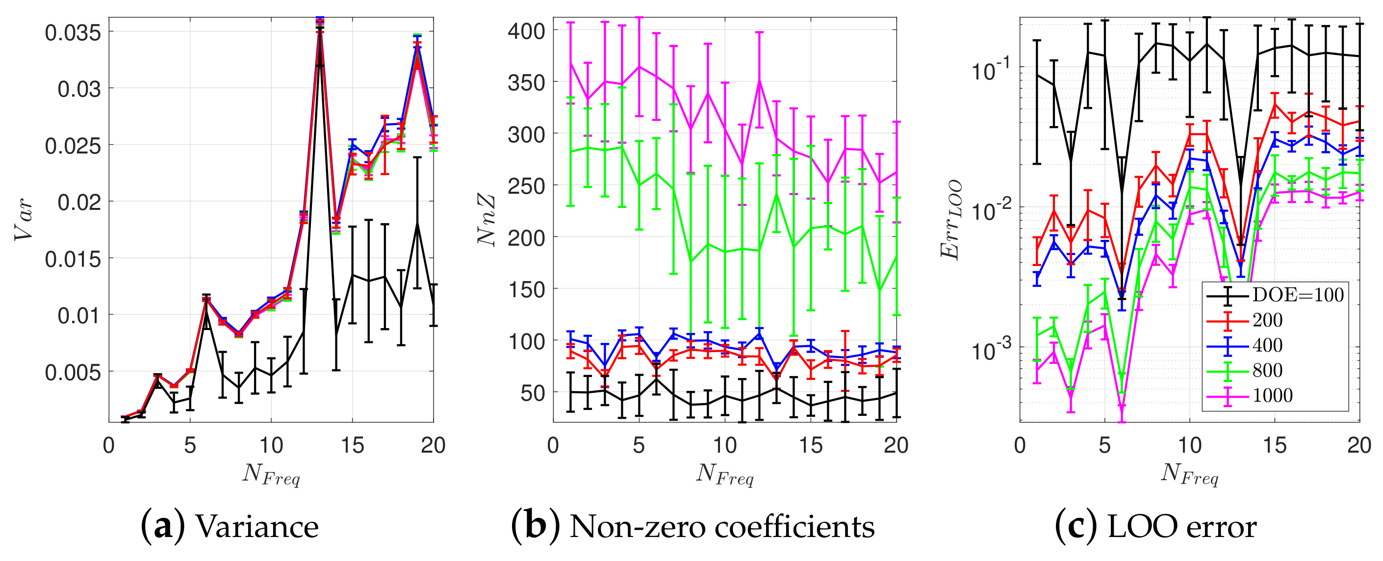
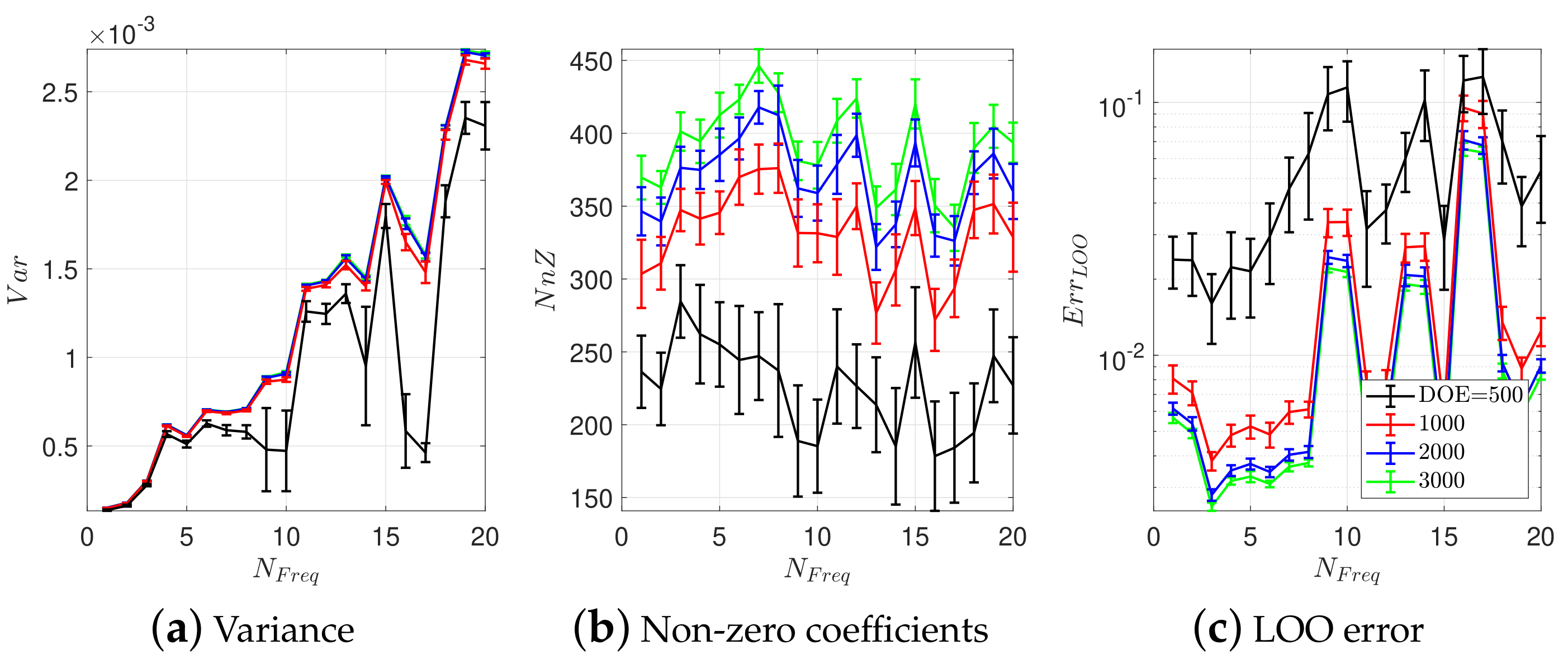
Finally, the impact of the DOE size on the quality of meta-model is studied in Figure 6 (only for the frequency response). The mean (not shown here) of different sample sizes are practically identical. The variance values have also similar trend for DOEs from 200 to 1000, while the model with DOE = 100 has different pattern; see Figure 6a. Increasing the DOE size, increases the number of NnZ coefficients; see Figure 6b. Finally, the LOO error decreases with an increase in the DOE size.

Next, the sensitivity of QoIs are computed with respect to the input RVs. The linear correlation is the simplest method to evaluate the sensitivity; however, it might be inaccurate in the presence of strongly nonlinear dependence between RVs. The Spearman’s rank correlation index, ${\rho }_S$, is a stable version which accounts for monotonicity instead of the linearity of the dependence between RVs. First, all the input and outputs are transformed into their rank-equivalents:

$$R_i=\left\{r_i^{\left(j\right)}\in \left\{1,\dots ,N\right\}:r_i^{\left(j\right)}>r_i^{\left(k\right)}\iff x_i^{\left(j\right)}>x_i^{\left(k\right)}\forall j,k\in \left\{1,\dots ,N\right\}\right\}.$$

(9)

In the same way, the rank-transformed model response is $R_Y=\left\{r_Y^{\left(1\right)},r_Y^{\left(2\right)},\dots ,r_Y^{\left(N\right)}\right\}$. Finally, the Spearman’s rank correlation indices are:

$${\rho }_{S_i}=\rho \left(R_i,R_Y\right)=\frac{\mathbb{E}\left[\left(R_i-{\mu }_i\right)\left(Y-{\mu }_{R_Y}\right)\right]}{{\sigma }_i{\sigma }_{R_Y}},$$

(10)

where $\mu$ is expectation of that quantity, and $\sigma$ refers to its standard deviation.

On the other hand, a direct outcome of a PCE-based surrogate model is to use the Sobol indices as a metric for sensitivity analysis. Decomposition of variance provides the sensitivity measures in the form of $S_{i_1,\dots ,i_s}$ which represent the relative contribution of each group of RVs $\left\{X_{i_1},\dots ,X_{i_s}\right\}$ to the total variance. The first order Sobol index is derived with respect to one RV $X_i$ (and its interaction with other RVs is neglected – which is referred to as high-order Sobol indices). In the functional form the sensitivity index is:

$$S_{i_1,\dots ,i_s}=\frac{D_{i_1,\dots ,i_s}}{D},$$

(11)

where the partial variances are:

$$D_{i_1,\dots ,i_s}=\int \dots \int f_{i_1,\dots ,i_s}^2\left(x_{i_1},\dots ,x_{i_s}\right)d{x}_{i_1}\dots d{x}_{i_s}1\le i_1\le \dots \le i_s\le M;s=1,\dots ,M,$$

(12)

where $f\left(\mathit{X}\right)$ presents the Sobol decomposition

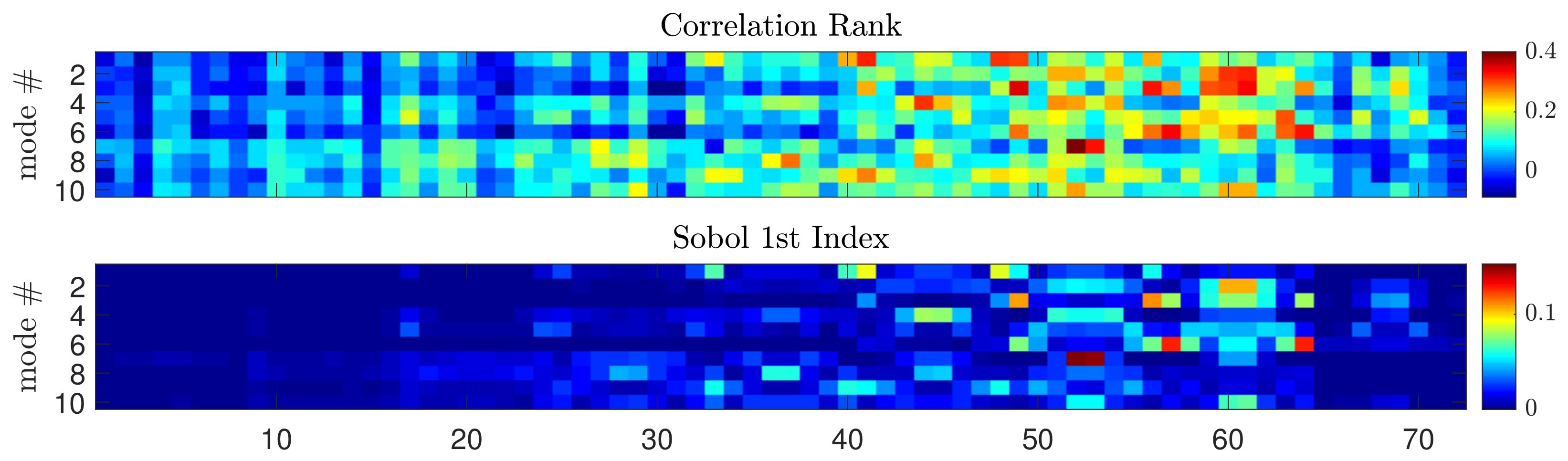
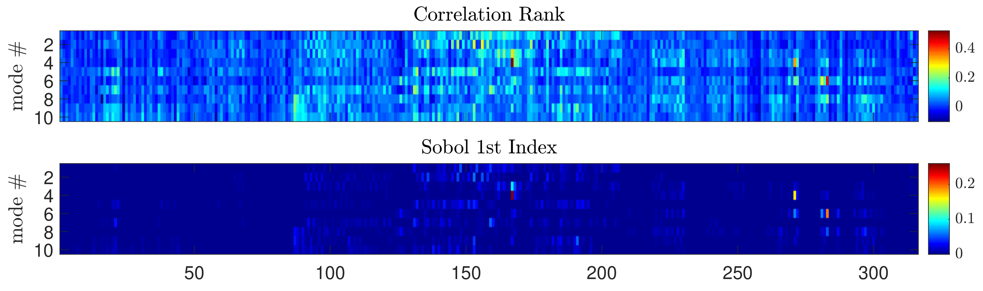
Figure 7 illustrates both the “Correlation Rank” and first order Sobol index for 10 frequencies and 72 RVs (which corresponds to spatial locations). As seen in this figure, the variation of colors which corresponds to sensitivity index is much higher in correlation rank method compared to first order Sobol index. Moreover, the correlation rank method has higher relative values. Estimation of the high sensitive RVs (locations) in both methods is close. It seems that the Sobol index filters more the RVs compared to correlation rank. Since each vibration mode is analyzed independent from others, the relative sensitivity index from one mode should not be compared to other modes (only the pattern is important).

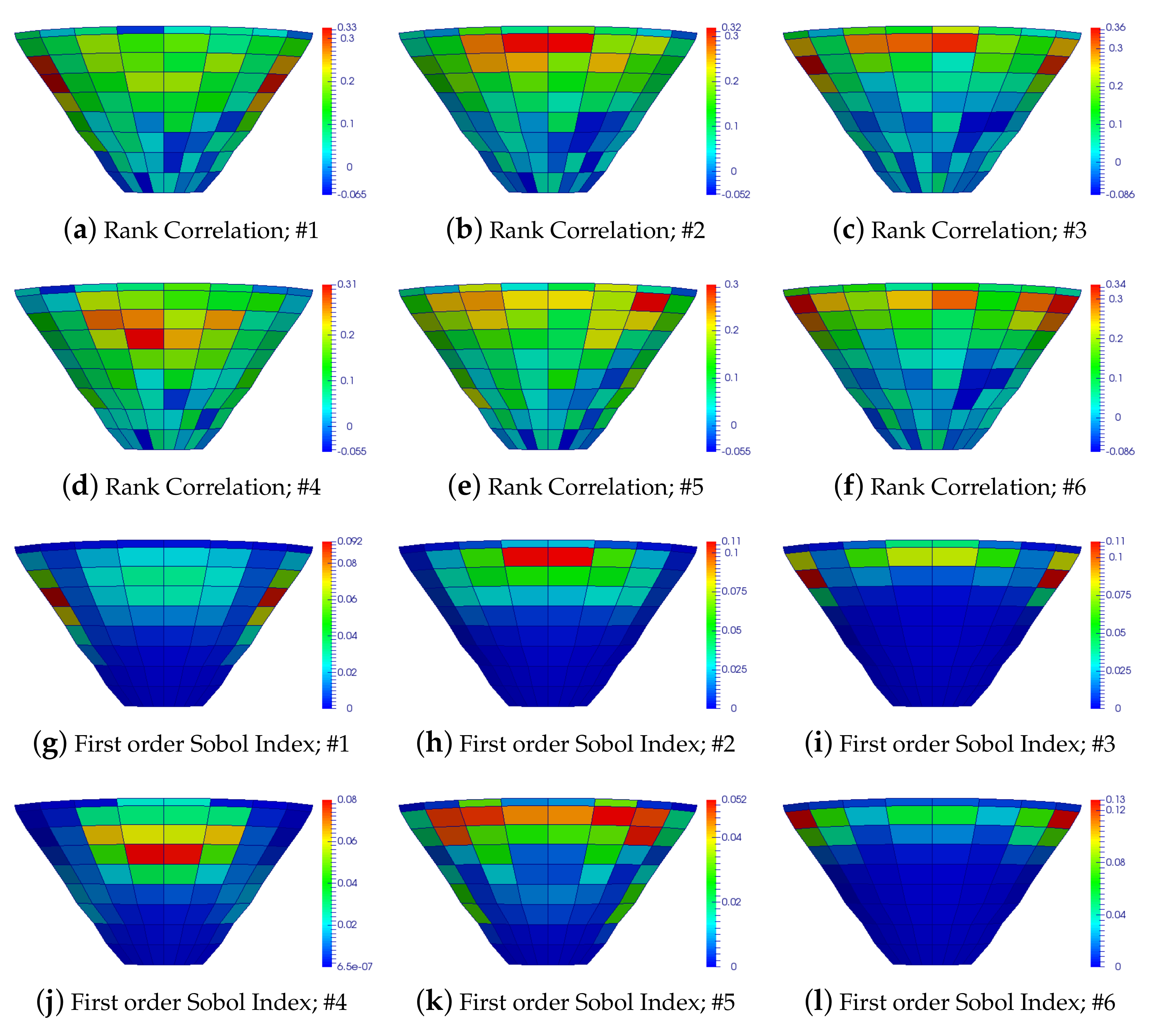
Figure 8 compares the spatial distribution of sensitivity indices for two methods and only first six modes of vibration. The main observations are as follows:

• In general, Correlation Rank provides a fair estimation of most sensitive locations compared to Sobol indices.
• Dam-1 is a symmetry dam with symmetry mesh, and it is expected the results of sensitivity analysis reflect this fact. However, the Correlation Rank method provides a non-uniform distribution of the sensitivity index within dam body. The results from Sobol index are quite symmetry.
• According to these figures, the regions of the dam in vicinity of abutments are most sensitive locations for the modes #1, #3, and #6. On the other hand, the middle regions located at the upper one-half are most sensitive for modes #2, #4, and #5. The lower half part of dam is not sensitive at all in its overall vibration characteristics.

Figure 8. Dam-1; Spatial distribution of sensitive location for different vibration modes.

Figure 8. Dam-1; Spatial distribution of sensitive location for different vibration modes.

4.2. Dam 2

A similar method as of Dam-1 is used for Dam-2. Figure 9 compares the response prediction via PCE (while the expansion coefficients will be omitted). Four initial (and deterministic) DOE values are considered, i.e., 500, 1000, 2000, and 3000. Aging, increasing the initial sample size, increases the accuracy of PCE meta-model, as well as the number of expansion coefficients. However, compared to Dam-1, the Dam-2 requires much more DOE to provide a good prediction. In addition, the performance of the PCE for frequency response seems to be better than effective mass (this was not the case in Dam-1).

Figure 9 only studied the 1st vibration mode. Therefore, the higher-modes effects will be evaluated by analyzing first 20 modes. A batch with 2000 initial DOEs is considered to be the pilot Dam-2 model. In each case, a similar PCE model as of mode #1 is generated; however with 20 replications (to reduce the potential uncertainty due to random selection of DOEs); see Figure 10.

According to Figure 10a,b, the mean and variance increase as a function of frequency (this response is similar to Dam-1). While the mean frequency has a quite uniform form, there are some nonlinear variations for the frequency variance (with some spikes). Based on Figure 10c, the non-zero coefficients are increased from initial about 340 to about 420 in mode #8. Then, it has a fluctuating behavior around 360 NnZ (this observation is different from Dam-1). Finally, the LOO error has also a non-uniform and non-constant pattern (as opposed to Dam-1); see Figure 10d.

Similar to Dam-1, in Dam-2, also, there is not a clear trend for the effective mass in the case of mean and variance response; see Figure 10e,f. Both the NnZ and LOO error have also a non-uniform pattern.

Finally, the impact of the DOE size on the quality of meta-model is studied in Figure 11 (only for the frequency response). The variance values have a similar trend for DOEs from 1000 to 3000, while the model with DOE = 500 is a bit different; see Figure 11a. Increasing the DOE size, increases the number of NnZ coefficients; see Figure 11b (as opposed to Dam-1, the variation of NnZ is nearly constant). Finally, the LOO error decreases with an increase in the DOE size (similar to Dam-1).

Figure 12 compares both the Correlation Rank and 1st Sobol index for 10 frequencies and 316 RVs (which corresponds to spatial locations). Again, variation of color contour is much more for Correlation Rank method compared to 1st Sobol index (which highlights only a few locations). Qualitatively, the predicted sensitive locations are different in two methods.

Figure 13 compares the spatial distribution of sensitivity indices for two methods using the first six modes of vibration. As opposed to Dam-1 in which there was only one layer of element withing the thickness, Dam-2 has two layers of elements. This provides the opportunity to investigate the curvature of mode shapes; thus, the sensitivity of the upstream and downstream side elements for various modes. The main observations are as follows:

• For this un-symmetry dam, the Correlation Rank method provides a good estimation of the most sensitive locations compared to the Sobol indices. For all six mode of vibrations, the most sensitive location is identical in two methods.
• It is observed that for some of the vibration modes, the estimated sensitive location at the upstream and downstream faces are different (modes #1, #2, and #5). For those modes, the First order Sobol indices are also illustrated on the downstream face (see Figure 13m–o). In modes #1 and #2, a central sensitive region in upstream face corresponds to two sensitive side areas in downstream face, and vice versa. This type of response is consistent with the nature of mode shapes in the shell-type structures.
• According to these figures, the upper central regions of upstream/downstream face (not in the vicinity of the crest), as well as the left bank, are the most sensitive locations.

Figure 13. Dam-2; Spatial distribution of sensitive location for different vibration modes.

Figure 13. Dam-2; Spatial distribution of sensitive location for different vibration modes.

4.3. Spectrum of Sensitivity Indices

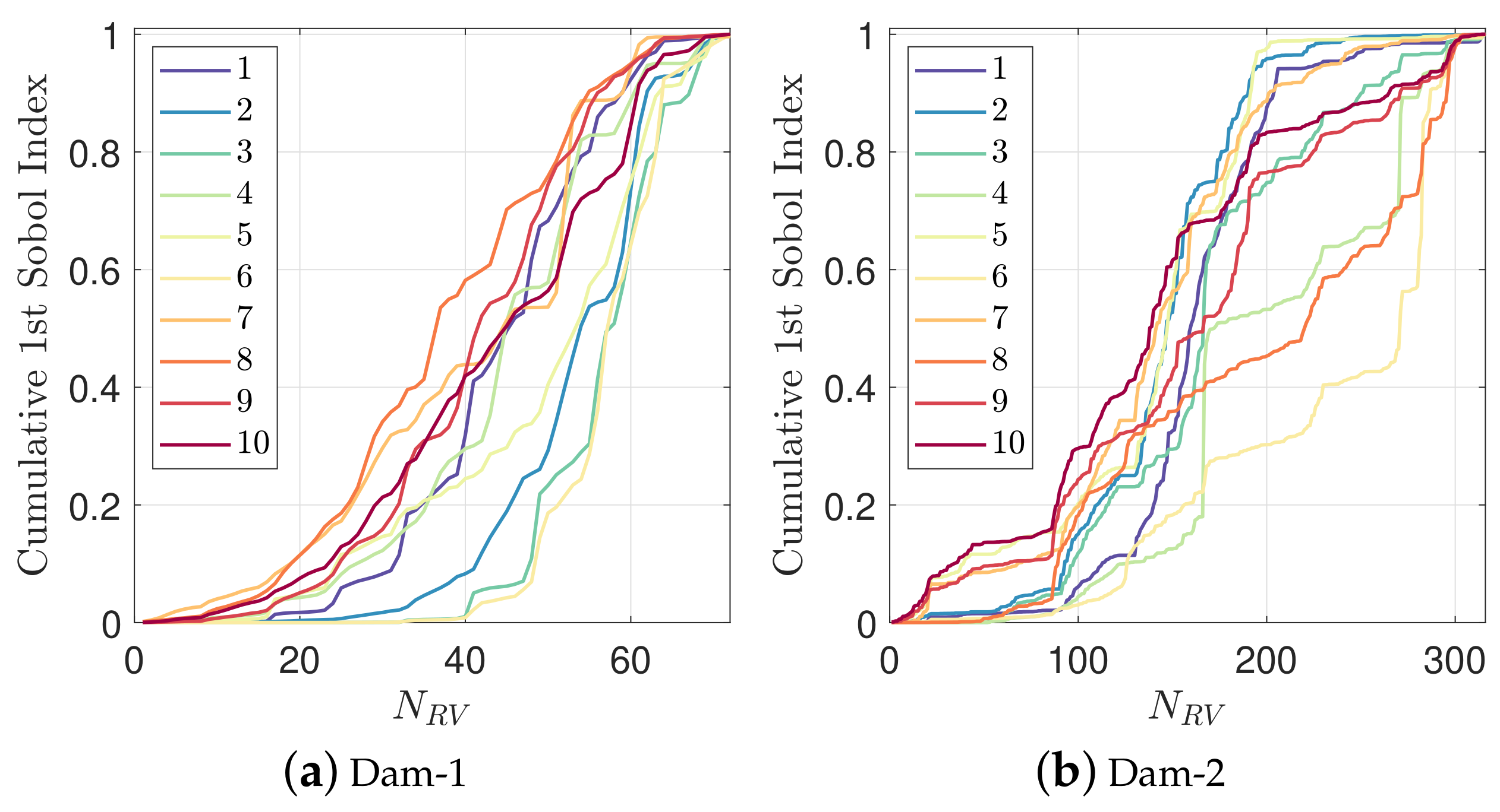
The summation of Sobol indices for all random variables is equal to one. Figure 14 summarizes the most important observations in this paper which is the spectrum of cumulative first order Sobol indices for the first 10 modes for each dam. Any sharp jump in these curves or a very steep slope indicate the importance of that particular random variable (i.e., location). These curves helps to identify the sensitive locations in dam for further inspection and potential instrumentation.

5. Results: Random Forest-Based Ensemble Regression

Random forest [41] is an ensemble method that builds a large collection of de-correlated trees, and then averages them [42]. Random forest is one of the base and standard methods in machine learning which is used in this section to validate further the results from PCE. Aside from random forest applications in classification and regression problems, it has a variable importance feature too. It is founded on the Out-of-Bag (OOB) data concept which refers to the samples that are not selected in bootstrapping in the random forest procedure. Error is then calculated by calculating random forest model with OOB data. Mathematically, the importance score (IS) is described as:

$$\mathrm{IS}=\frac{1}{N_t}\sum _{j=1}^B\left(E_j-E_j^{\ast }\right),$$

(13)

where $N_t$ is the number of trees in the model, and $E_j$ and $E_j^{\ast }$ are the errors of each tree applied on OOB and perturbed OOB data, respectively. This method has been implemented on the data from both dams using the “randomForest” function [43] available in R with “ntree = 500”.

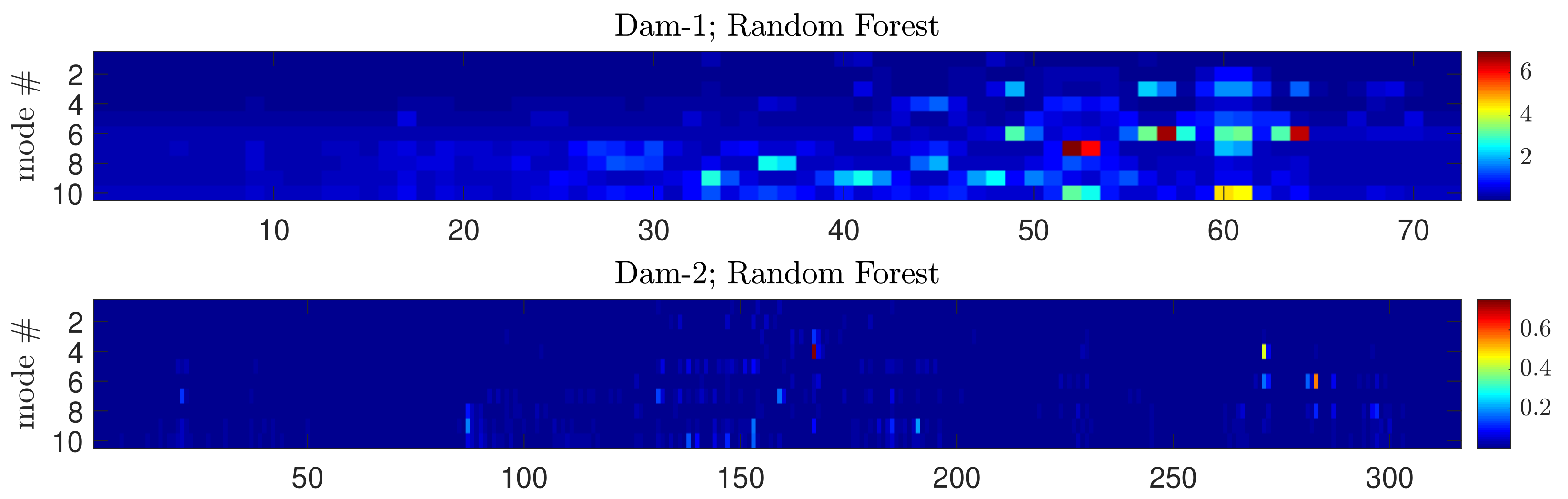
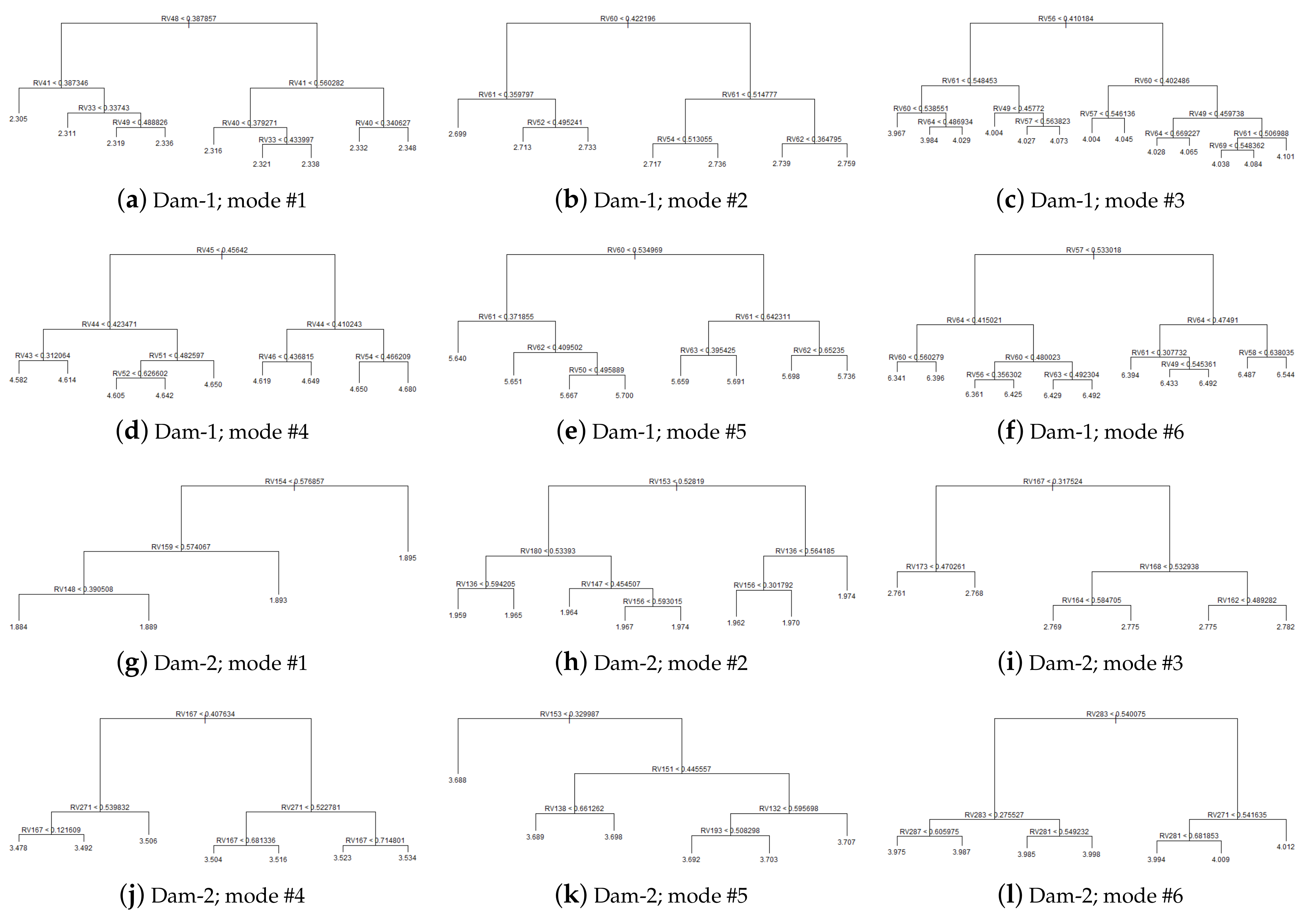
Figure 15 presents the estimated variable importance by random forest method for two dams. In general, the random forest pattern is similar to PCE rather than Correlation Rank. In addition, it seems that random forest assigns higher weight to some RVs (regions) and, thus, filters less important variables. In random forest, the local variable importance is shown graphically shown using tress. Tree can be shown either based on absolute or relative values. Figure A2 presents trees for first six modes of Dam-1 and Dam-2 based on the normalized modulus of elasticity value (which has a heterogeneous distribution). At any regression tree, the value of the random variable (in this case, 1 to 72 for Dam-1 and 1 to 316 for Dam-2 in the form of RV$\ast \ast \ast$) is checked, and depending of the (binary) answer, the tree grows to the left or right sub-branch. Once a tree reaches to any of its leaves, the estimated value (in this case, the vibration frequency) is obtained. As opposed to linear or polynomial regression, which are global models (the meta-model is supposed to hold in the entire data space), trees partition the data space into small enough parts where one may apply a simple different model on each part.

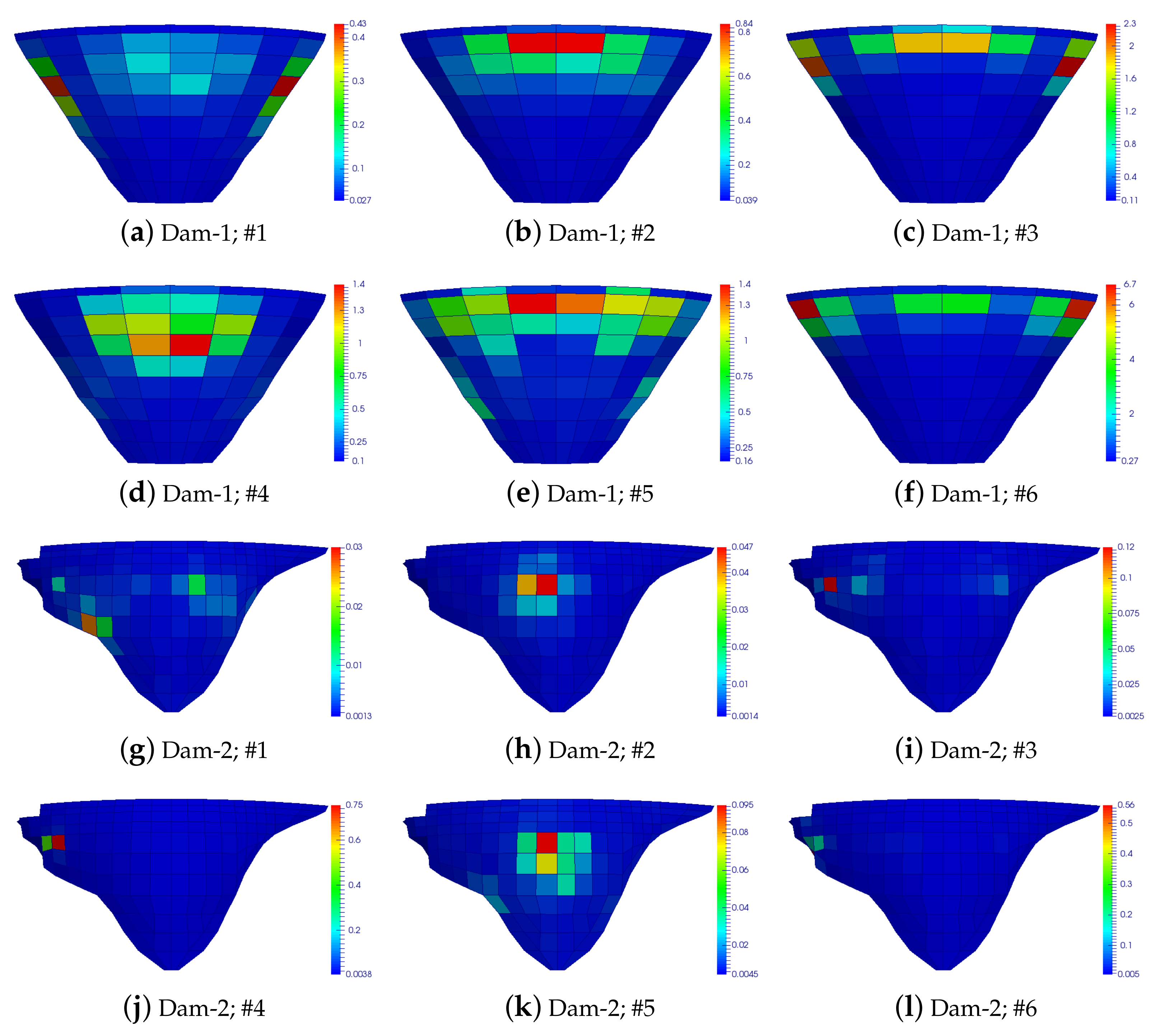
Figure 16 illustrates the spatial distribution of variable importance for both dams based on random forest method. In general, random forest provides the spatial distribution in a very similar way to first order Sobol index. The only difference is that first order Sobol index provided a complete symmetry sensitivity prediction for Dam-1, while random forest exhibits small un-symmetry behavior (in any case is un-symmetry level is much less that Correlation Rank estimation). In the case of Dam-2, it seems that random forest filters even more the insensitive RVs (regions) and strictly focuses on few highly important RVs.

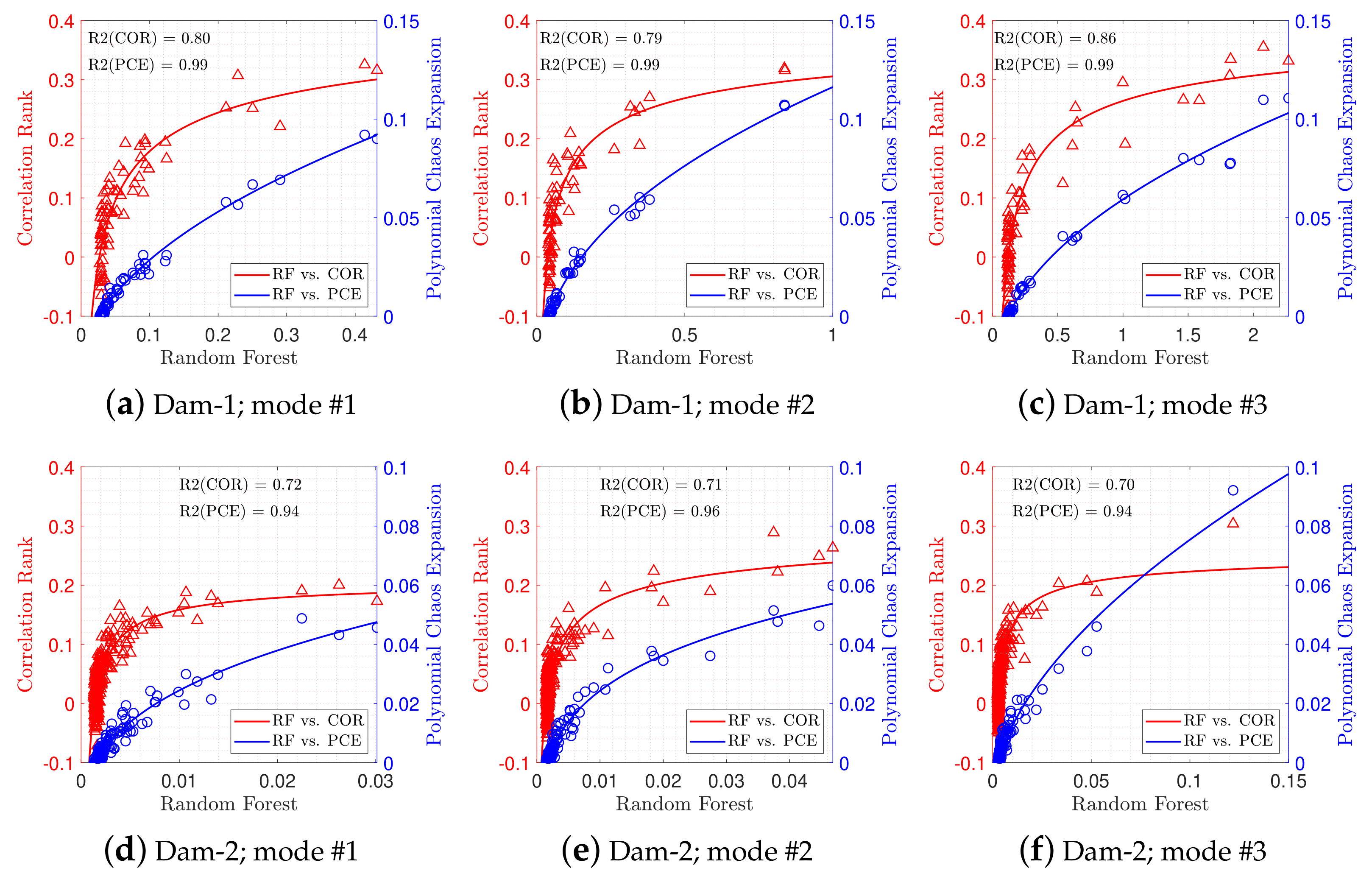
Finally, Figure 17 compares the relative importance of RVs (72 RVs in Dam-1 and 316 RVs in Dam-2) from random forest (horizontal axis) with correlation Rank (left vertical axis) and PCE-based first order Sobol index (right vertical axis). As seen, there is a high correlation between random forest and PCE and coefficient of determination (R2) of 0.99 for Dam-1 and 0.95 for Dam-2. On the other hand, the random forest is less correlated with Correlation Rank method and the average of R2 is about 0.85 for Dam-1 and 0.70 for Dam-2. The reported goodness-of-fit metrics are based on a fitted power-form equation, $a{x}^b+c$, which shows a completely nonlinear relation between Correlation Rank and random forest, and a semi-linear one between PCE and random forest.

6. Connection to the System Identification and Dynamic Analysis

Arch dams are three-dimensional shell-type structures with a large degree of indeterminacy. Anatomy of vibration in concrete arch dams is complex and requires special techniques to solve the eigenvalue problems. Typically, the material properties in concrete are assumed to be isotropic and homogeneous which facilitates the coupled modal analysis. However, it is well-accepted that the material properties within the dams (and in general any the large-scale infra-structures) is not quite homogeneous.

The structural-level heterogeneity might be due to differences in concreting in large scale, or deterioration/aging over the time. The latter one is typically observed in dams due to alkali aggregate reaction. The concrete heterogeneity will alter the vibration nature of the structure (compared to the homogeneous one) [44]. The U.S. bureau of reclamation [9] conducted a series of seismic tomography tests on Seminoe Dam, located in Wyoming, which is suffering from ASR. While the lower parts of the dam have a modulus of elasticity of about 20 GPa, it reduces to only 9 GPa in the vicinity of crest with a highly heterogeneous pattern. Custódio et al. [45] studied the performance of 80 m high Miranda buttress dam. Evidences of AAR has been found due to progressive vertical displacements upwards, as well as vertical sliding on the central contraction joints. The cylindrical test results, show that there is a great variability on the condition of the concrete sampled throughout the structure. Compressive strength is ranging from 20 to 48 MPa; tensile splitting test from 1.7 to 4.1 MPa; and stiffness damage test from 23 to 37 GPa.

The outcome of this study can improve the results of dynamic analysis in different aspects. During the model calibration (e.g., based on forced vibration test), the results of sensitivity analysis help to minimize the computational time for system identification by mainly focusing on the most important regions. In this approach, instead of assigning thousands potential heterogeneous patterns to the dam body, the calibration is only conducted by searching the right material properties in the sensitive regions for that particular vibration mode.

Next, the outcome is used in dynamic analysis. Two widely used finite element dynamic analysis techniques for concrete dams are: response spectrum analysis and time integration method.

• In the response spectrum analysis technique, the response of the coupled system (i.e., displacement and stress) is separately computed for each vibration mode, and then are combined to calculate the total system level response. Using a proper heterogeneous model with exact effective mass and participation factor improves the accuracy of total calculations. In addition, it is important to identify the most effective vibration modes which contribute most to the dynamic response of the system. The number of effective modes (which might be different in heterogeneous models compared to the homogeneous ones) is typically selected to reach at least 90% total accuracy.
• In the time-integration time history analysis, the heterogeneous dam assumption alters the stiffness matrix and damping values of at different modes.

7. Summary and Conclusions

Quantification of structural vibration characteristics is an essential task prior to perform any dynamic health monitoring, and system identification. Most of the finite element models are validated based on the vibration characteristics of the dam, thus ignoring concrete heterogeneity may lead to poor/wrong model validation.

This paper proposed a hybrid random field—polynomial chaos expansion surrogate model for uncertainty quantification and sensitivity assessment of dam structures. First, an efficient random fields model is developed and the concrete heterogeneity is simulated. Next, two dam models (symmetry and un-symmetry) are selected and a large number of eigenvalue analyses were performed on the models. From the analyses, the vibration characteristics (i.e., frequencies, effective masses, and participation factors) were extracted. This large database is used to develop a PCE-based surrogate model. A natural outcome of such a meta-model is to quantify the Sobol indices in various random variables (in this case, different locations). This is a great metric to identify the most sensitive dam locations for different vibration modes.

Another important conclusion in this figure is that the general trend of a symmetry dam is different from a un-symmetry one because in the former one the modes are well-separated, while, in the latter case, the modes are interacting. Comparing the PCE-based sensitivity analysis with correlation rank method showed that the latter one does not provide a reliable estimate of the important random variables. Furthermore, the results of the proposed hybrid model is validated using the classical random forest regression method, and a good consistency has been reported.

References

- Hariri-Ardebili, M.; Kianoush, M. Integrative seismic safety evaluation of a high concrete arch dam. Soil Dyn. Earthq. Eng. 2014, 67, 85–101. [Google Scholar] [CrossRef]
- Oliveira, S.; Alegre, A. Seismic and structural health monitoring of dams in Portugal. In Seismic Structural Health Monitoring; Springer: Berlin/Heidelberg, Germany, 2019; pp. 87–113. [Google Scholar]
- Oliveira, S.; Alegre, A. Seismic and structural health monitoring of Cabril dam. Software development for informed management. J. Civ. Struct. Health Monit. 2020, 10, 913–925. [Google Scholar] [CrossRef]
- Yang, J.; Jin, F.; Wang, J.T.; Kou, L.H. System identification and modal analysis of an arch dam based on earthquake response records. Soil Dyn. Earthq. Eng. 2017, 92, 109–121. [Google Scholar] [CrossRef]
- Gomes, J.P.; Lemos, J.V. Characterization of the dynamic behavior of a concrete arch dam by means of forced vibration tests and numerical models. Earthq. Eng. Struct. Dyn. 2020, 49, 679–694. [Google Scholar] [CrossRef]
- Bukenya, P.; Moyo, P.; Beushausen, H.; Oosthuizen, C. Health monitoring of concrete dams: A literature review. J. Civ. Struct. Health Monit. 2014, 4, 235–244. [Google Scholar] [CrossRef]
- Sevieri, G.; De Falco, A. Dynamic structural health monitoring for concrete gravity dams based on the Bayesian inference. J. Civ. Struct. Health Monit. 2020, 10, 235–250. [Google Scholar] [CrossRef] [Green Version]
- Alves, S.; Hall, J. System identification of a concrete arch dam and calibration of its finite element model. Earthq. Eng. Struct. Dyn. 2006, 35, 1321–1337. [Google Scholar] [CrossRef]
- Dam Safety Office. Seismic Tomography of Concrete Structures; Report No. DSO-02-03; Technical Report; Department of the Interior, Bureau of Reclamation: Denver, CO, USA, 2002.
- Hariri-Ardebili, M.; Seyed-Kolbadi, S.; Saouma, V.; Salamon, J.; Nuss, L. Anatomy of the vibration characteristics in old arch dams by random field theory. Eng. Struct. 2019, 179, 460–475. [Google Scholar] [CrossRef]
- Hariri-Ardebili, M.A. Safety and reliability assessment of heterogeneous concrete components in nuclear structures. Reliab. Eng. Syst. Saf. 2020, 203, 107104. [Google Scholar] [CrossRef]
- Guo, X.; Dias, D.; Carvajal, C.; Peyras, L.; Breul, P. Reliability analysis of embankment dam sliding stability using the sparse polynomial chaos expansion. Eng. Struct. 2018, 174, 295–307. [Google Scholar] [CrossRef]
- Sevieri, G.; Andreini, M.; De Falco, A.; Matthies, H.G. Concrete gravity dams model parameters updating using static measurements. Eng. Struct. 2019, 196, 109231. [Google Scholar] [CrossRef]
- Hariri-Ardebili, M.; Sudret, B. Polynomial chaos expansion for uncertainty quantification of dam engineering problems. Eng. Struct. 2020, 203, 109631. [Google Scholar] [CrossRef]
- Kim, Y.J. Comparative study of surrogate models for uncertainty quantification of building energy model: Gaussian Process Emulator vs. Polynomial Chaos Expansion. Energy Build. 2016, 133, 46–58. [Google Scholar] [CrossRef]
- Wei, X.; Wan, H.P.; Russell, J.; Živanović, S.; He, X. Influence of mechanical uncertainties on dynamic responses of a full-scale all-FRP footbridge. Compos. Struct. 2019, 223, 110964. [Google Scholar] [CrossRef]
- Slot, R.M.; Sørensen, J.D.; Sudret, B.; Svenningsen, L.; Thøgersen, M.L. Surrogate model uncertainty in wind turbine reliability assessment. Renew. Energy 2020, 151, 1150–1162. [Google Scholar] [CrossRef] [Green Version]
- Ni, P.; Xia, Y.; Li, J.; Hao, H. Using polynomial chaos expansion for uncertainty and sensitivity analysis of bridge structures. Mech. Syst. Signal Process. 2019, 119, 293–311. [Google Scholar] [CrossRef]
- Bouhjiti, D.M.; Baroth, J.; Dufour, F.; Michel-Ponnelle, S.; Masson, B. Stochastic finite elements analysis of large concrete structures’ serviceability under thermo-hydro-mechanical loads—Case of nuclear containment buildings. Nucl. Eng. Des. 2020, 370, 110800. [Google Scholar] [CrossRef]
- Dubreuil, S.; Bartoli, N.; Gogu, C.; Lefebvre, T.; Colomer, J.M. Extreme value oriented random field discretization based on an hybrid polynomial chaos expansion—Kriging approach. Comput. Methods Appl. Mech. Eng. 2018, 332, 540–571. [Google Scholar] [CrossRef]
- Guo, X.; Dias, D.; Carvajal, C.; Peyras, L.; Breul, P. A comparative study of different reliability methods for high dimensional stochastic problems related to earth dam stability analyses. Eng. Struct. 2019, 188, 591–602. [Google Scholar] [CrossRef]
- Guo, X.; Dias, D.; Pan, Q. Probabilistic stability analysis of an embankment dam considering soil spatial variability. Comput. Geotech. 2019, 113, 103093. [Google Scholar] [CrossRef]
- Mishra, M.; Keshavarzzadeh, V.; Noshadravan, A. Reliability-based lifecycle management for corroding pipelines. Struct. Saf. 2019, 76, 1–14. [Google Scholar] [CrossRef]
- Ghanem, R.G.; Spanos, P.D. Stochastic Finite Elements: A Spectral Approach; Courier Corporation: North Chelmsford, MA, USA, 2003. [Google Scholar]
- Fajraoui, N.; Marelli, S.; Sudret, B. Sequential Design of Experiment for Sparse Polynomial Chaos Expansions. SIAM/ASA J. Uncertain. Quantif. 2017, 5, 1061–1085. [Google Scholar] [CrossRef]
- Blatman, G.; Sudret, B. Adaptive sparse polynomial chaos expansion based on least angle regression. J. Comput. Phys. 2011, 230, 2345–2367. [Google Scholar] [CrossRef]
- Cavazzuti, M. Optimization Methods: From Theory to Design Scientific and Technological Aspects in Mechanics; Springer Science & Business Media: Berlin/Heidelberg, Germany, 2012. [Google Scholar]
- Efron, B.; Hastie, T.; Johnstone, I.; Tibshirani, R. Least angle regression. Ann. Stat. 2004, 32, 407–499. [Google Scholar]
- Blatman, G.; Sudret, B. An adaptive algorithm to build up sparse polynomial chaos expansions for stochastic finite element analysis. Probabilistic Eng. Mech. 2010, 25, 183–197. [Google Scholar] [CrossRef]
- Vanmarcke, E. Random Fields: Analysis and Synthesis; The MIT Press: Cambridge, MA, USA, 1983. [Google Scholar]
- Hariri-Ardebili, M.; Seyed-Kolbadi, S.; Saouma, V.; Salamon, J.; Rajagopalan, B. Random finite element method for the seismic analysis of gravity dams. Eng. Struct. 2018, 171, 405–420. [Google Scholar] [CrossRef]
- Der Kiureghian, A.; Ke, J.B. The stochastic finite element method in structural reliability. Probabilistic Eng. Mech. 1988, 3, 83–91. [Google Scholar] [CrossRef]
- Olsson, A.; Sandberg, G. Latin hypercube sampling for stochastic finite element analysis. J. Eng. Mech. 2002, 128, 121–125. [Google Scholar] [CrossRef]
- Hernandez, V.; Roman, J.; Tomas, A.; Vidal, V. A Survey of Software for Sparse Eigenvalue Problems; SLEPc Technical Report STR-6; Universitat Politecnica de Valencia: Valencia, Spain, 2009. [Google Scholar]
- Lanczos, C. An Iteration Method for the Solution of the Eigenvalue Problem of Linear Differential and Integral Operators; United States Governm. Press Office: Los Angeles, CA, USA, 1950.
- Newman, M.; Ojalvo, I. Vibration modes of large structures by an automatic matrix-reduction method. AIAA J. 1970, 8, 1234–1239. [Google Scholar]
- Cullum, J.K.; Willoughby, R.A. Lanczos Algorithms for Large Symmetric Eigenvalue Computations: Vol. I: Theory; SIAM: Philadelphia, PA, USA, 2002. [Google Scholar]
- Saad, Y. Numerical Methods for Large Eigenvalue Problems; Manchester University Press: Manchester, UK, 1992. [Google Scholar]
- Sudret, B. Uncertainty Propagation and Sensitivity Analysis in Mechanical Models—Contributions to Structural Reliability and Stochastic Spectral Methods; Habilitationa Diriger des Recherches, Université Blaise Pascal: Clermont-Ferrand, France, 2007; p. 18. [Google Scholar]
- Marelli, S.; Sudret, B. UQLab: A framework for uncertainty quantification in Matlab. In Vulnerability, Uncertainty, and Risk: Quantification, Mitigation, and Management; ASCE: Reston, VA, USA, 2014; pp. 2554–2563. [Google Scholar]
- Breiman, L. Random forests. Mach. Learn. 2001, 45, 5–32. [Google Scholar] [CrossRef] [Green Version]
- Friedman, J.; Hastie, T.; Tibshirani, R. The Elements of Statistical Learning; Springer: New York, NY, USA, 2001. [Google Scholar]
- Breiman, L. Randomforest: Breiman and Cutler’s Random Forests for Classification and Regression; R Package Version 4.6-12; R Team: Vienna, Austria, 2015. [Google Scholar]
- Saouma, V.; Hariri-Ardebili, M.; Graham-Brady, L. Stochastic Analysis of Concrete Dams with Alkali Aggregate Reaction. Cem. Concr. Res. 2020, 132, 106032. [Google Scholar] [CrossRef]
- Custódio, j.; Ferreira, j.; Silva, A.; Ribeiro, A.; Batista, A. The diagnosis and prognosis of ASR and ISR in Miranda dam, Portugal. In Swelling Concrete in Dams and Hydraulic Structures: DSC 2017; Sellier, A., Grimal, É., Multon, S., Bourdarot, E., Eds.; John Wiley & Sons: Hoboken, NJ, USA, 2017. [Google Scholar]
Figure 1.
Sample random fields generation and its finite element discretization.
Figure 2.
A framework for uncertainty quantification with random fields; adapted from Reference [40] and expanded.
Figure 3.
Finite element model of the case study dams with main dimensions (not to scale).
Figure 4.
Dam-1; Polynomial Chaos Expansion (PCE)-based surrogate models for varying number of initial DOEs = 100, 200, 400, 800, and 1000 (left to right).
Figure 5.
Dam-1; Probabilistic PCE-based surrogate models for different vibration frequencies and quantity of interests (QoIs) all with 800 DOE; ω: frequency.
Figure 6.
Dam-1; impact of DOE size on the PCE-based surrogate models for frequency response.
Figure 7.
Dam-1; comparison of sensitivity indices for two methods and 10 modes.
Figure 9.
Dam-2; PCE-based surrogate models for varying number of initial DOEs.
Figure 10.
Dam-2; Probabilistic PCE-based surrogate models for different vibration frequencies and QoIs all with 2000 DOE.
Figure 11.
Dam-2; impact of DOE size on the PCE-based surrogate models for frequency response.
Figure 12.
Dam-2; comparison of sensitivity indices for two methods and 10 modes.
Figure 14.
Spectrum of cumulative first order Sobol indices along number of random variables, NRV, for various modes.
Figure 15.
Estimation of variable importance using random forest for two dams and 10 modes.
Figure 16.
Random forest-based spatial distribution of sensitive location for different vibration modes in Dam-1 and Dam-2.
Figure 17.
Correlation among three sensitivity metrics for various vibration modes.
Publisher’s Note: MDPI stays neutral with regard to jurisdictional claims in published maps and institutional affiliations. |
© 2021 by the authors. Licensee MDPI, Basel, Switzerland. This article is an open access article distributed under the terms and conditions of the Creative Commons Attribution (CC BY) license (http://creativecommons.org/licenses/by/4.0/).
Share and Cite
MDPI and ACS Style
Hariri-Ardebili, M.A.; Mahdavi, G.; Abdollahi, A.; Amini, A. An RF-PCE Hybrid Surrogate Model for Sensitivity Analysis of Dams. Water 2021, 13, 302. https://doi.org/10.3390/w13030302
AMA Style
Hariri-Ardebili MA, Mahdavi G, Abdollahi A, Amini A. An RF-PCE Hybrid Surrogate Model for Sensitivity Analysis of Dams. Water. 2021; 13(3):302. https://doi.org/10.3390/w13030302
Chicago/Turabian StyleHariri-Ardebili, Mohammad Amin, Golsa Mahdavi, Azam Abdollahi, and Ali Amini. 2021. "An RF-PCE Hybrid Surrogate Model for Sensitivity Analysis of Dams" Water 13, no. 3: 302. https://doi.org/10.3390/w13030302
Note that from the first issue of 2016, this journal uses article numbers instead of page numbers. See further details here.