
The Significance of Vertical and Lateral Groundwater–Surface Water Exchange Fluxes in Riverbeds and Riverbanks: Comparing 1D Analytical Flux Estimates with 3D Groundwater Modelling

 , , , and
Abstract
:1. Introduction
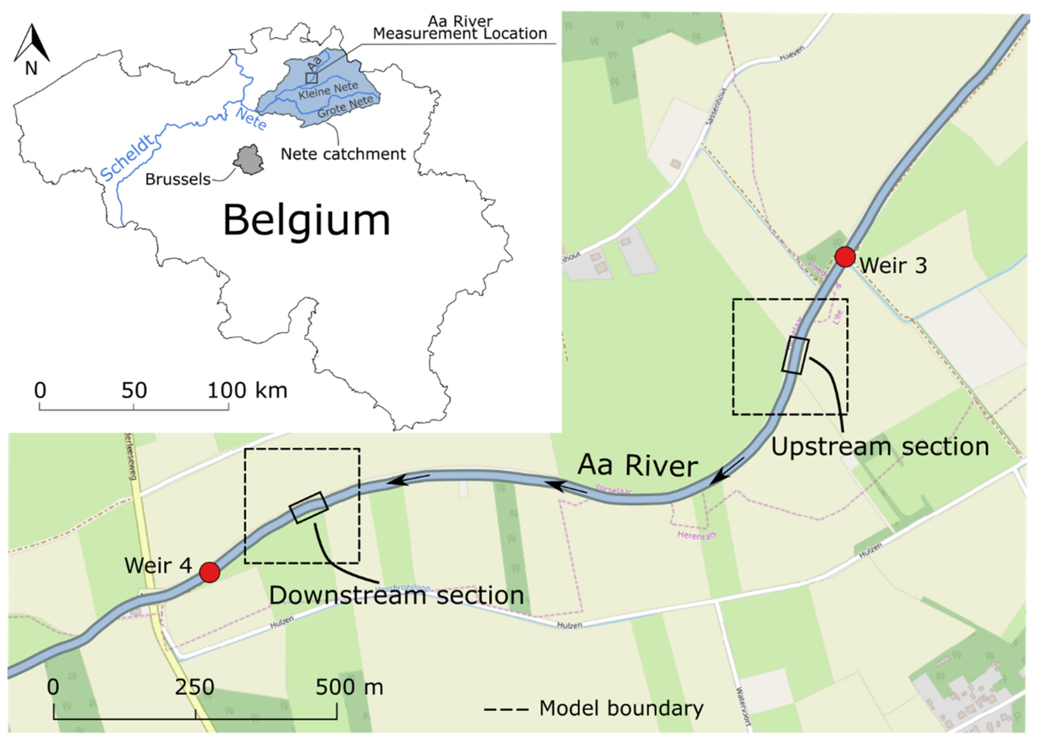
2. Study Area and Field Measurements
3. Methodology
3.1. Temperature Measurements
3.2. Vertical Exchange Flux Estimates from Riverbed Temperature Profiles
3.3. Variogram Analysis and Spatial Interpolation
3.4. Groundwater Flow Modelling
4. Results and Discussion
4.1. Vertical Exchange Flux Estimates Based on 1D Analytical Solution
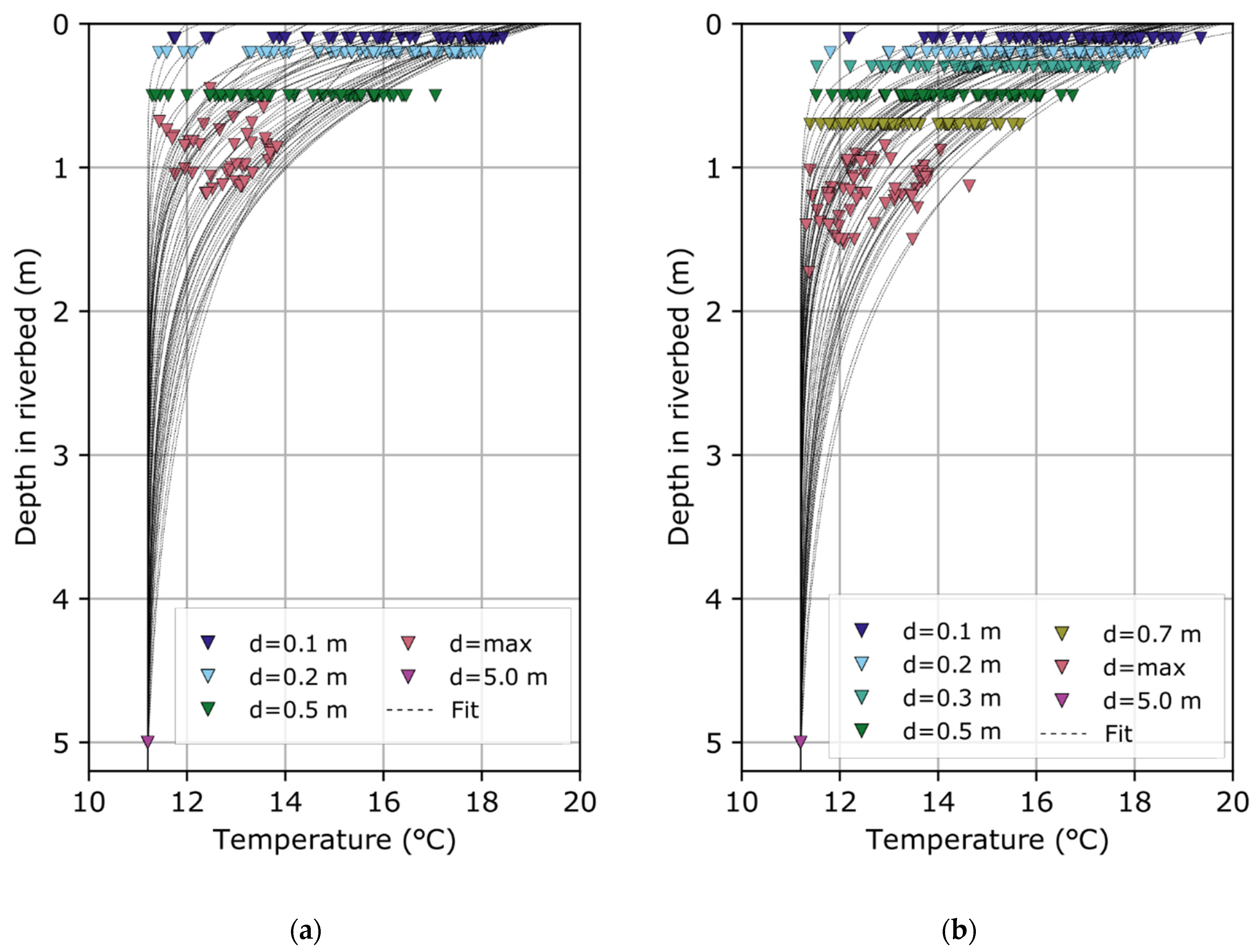
4.1.1. Temperature Measurements with T-Lance
4.1.2. Point-In-Space 1D-Flux Estimates
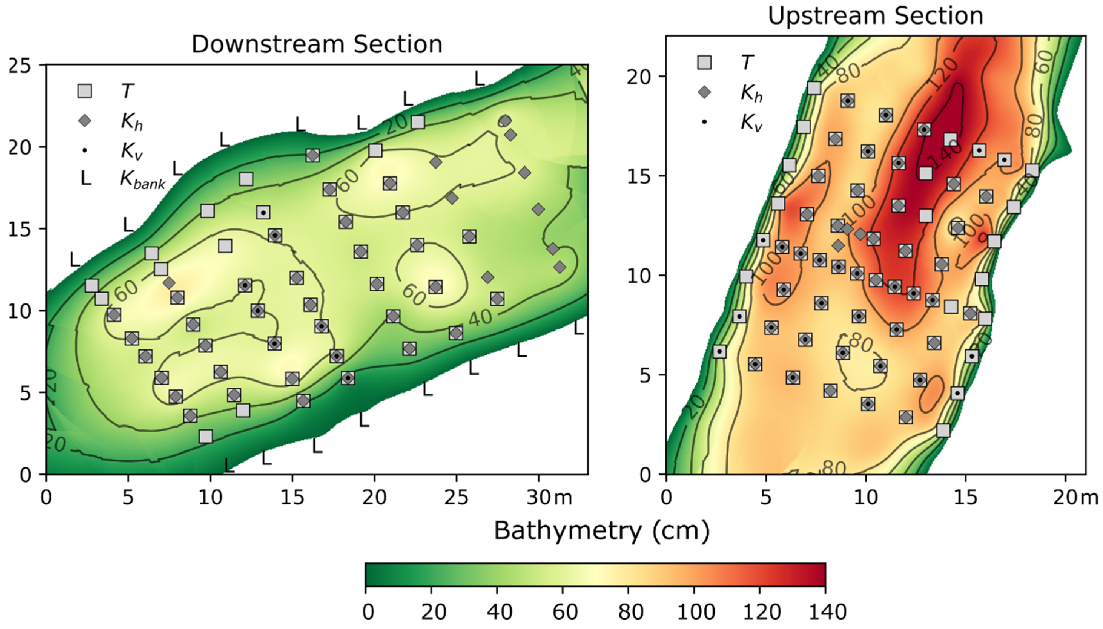
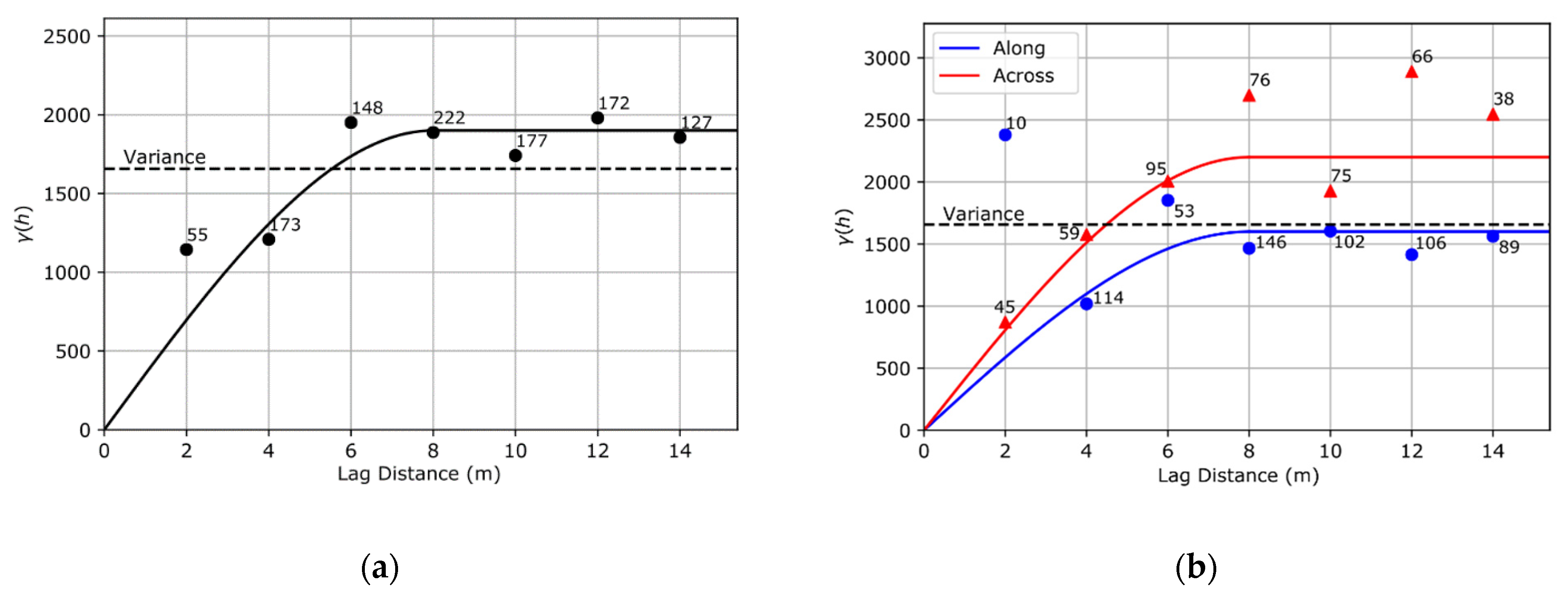
4.1.3. Spatial Variability and Anisotropy
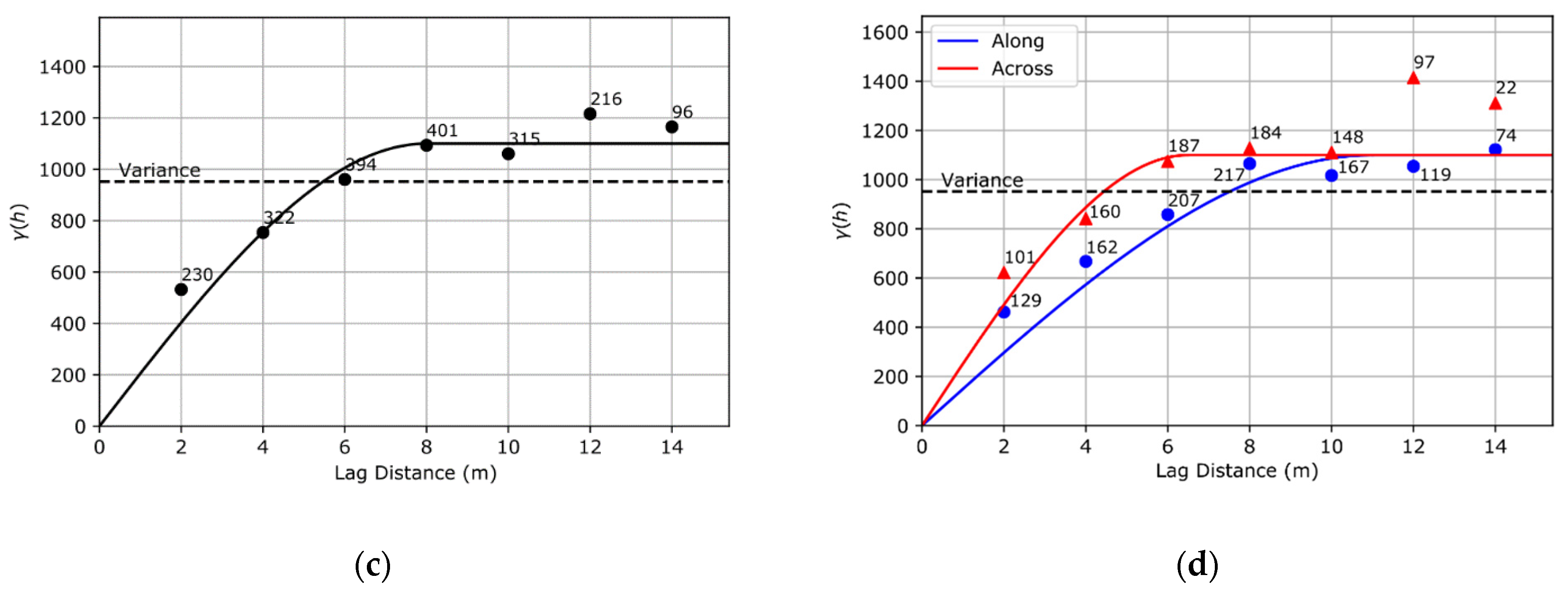
4.1.4. Correlation to Riverbed Hydraulic Conductivity
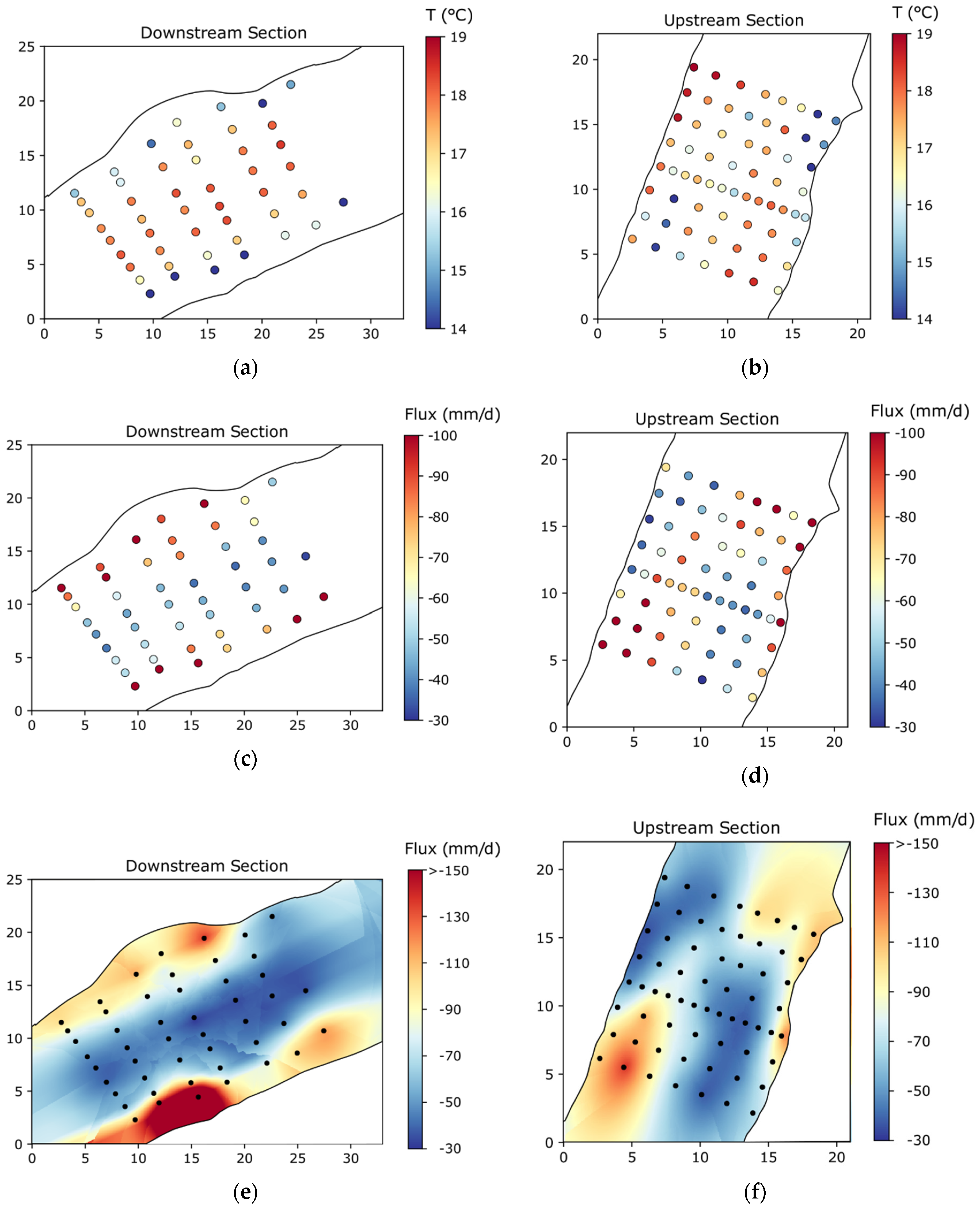
4.2. Fluxes from Groundwater Flow Modelling
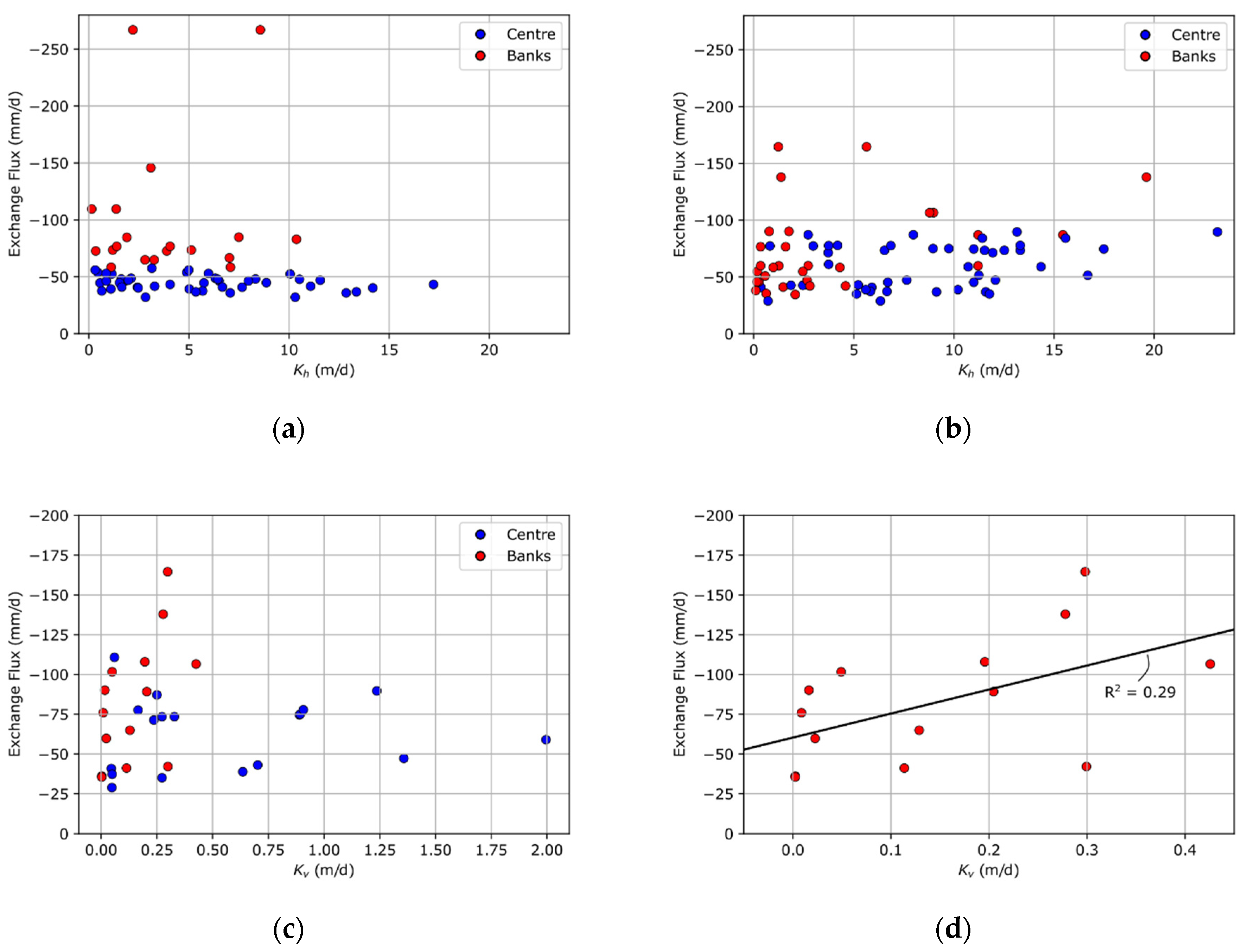
4.2.1. Downstream Section
4.2.2. Upstream Section
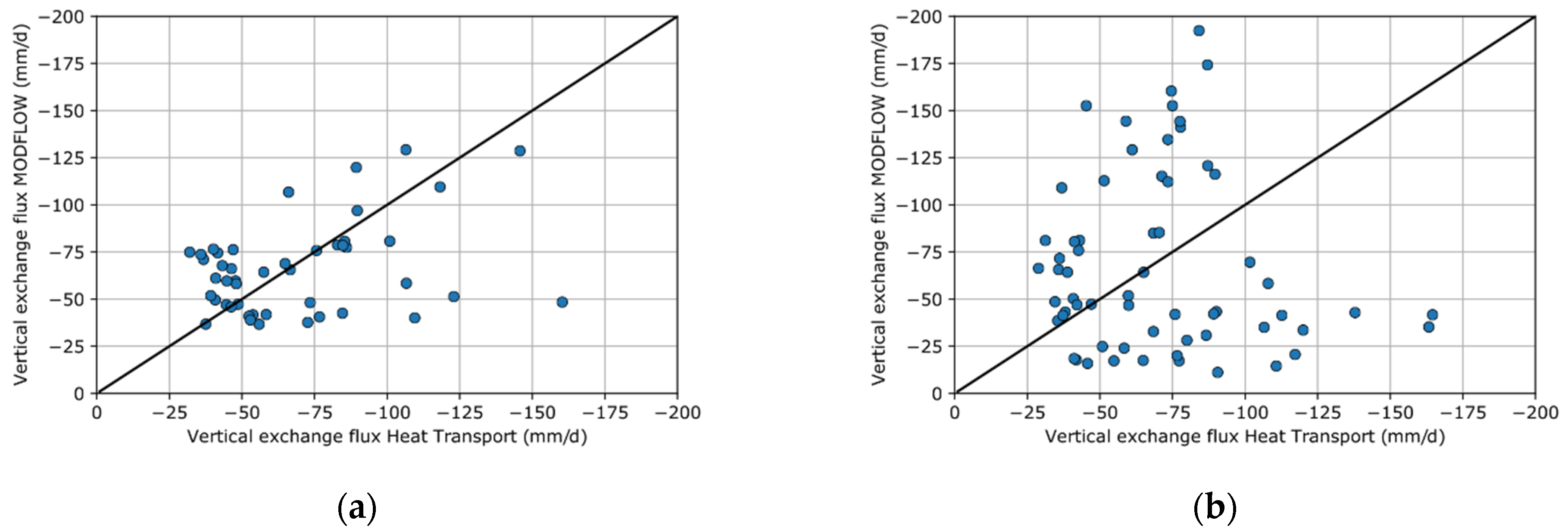
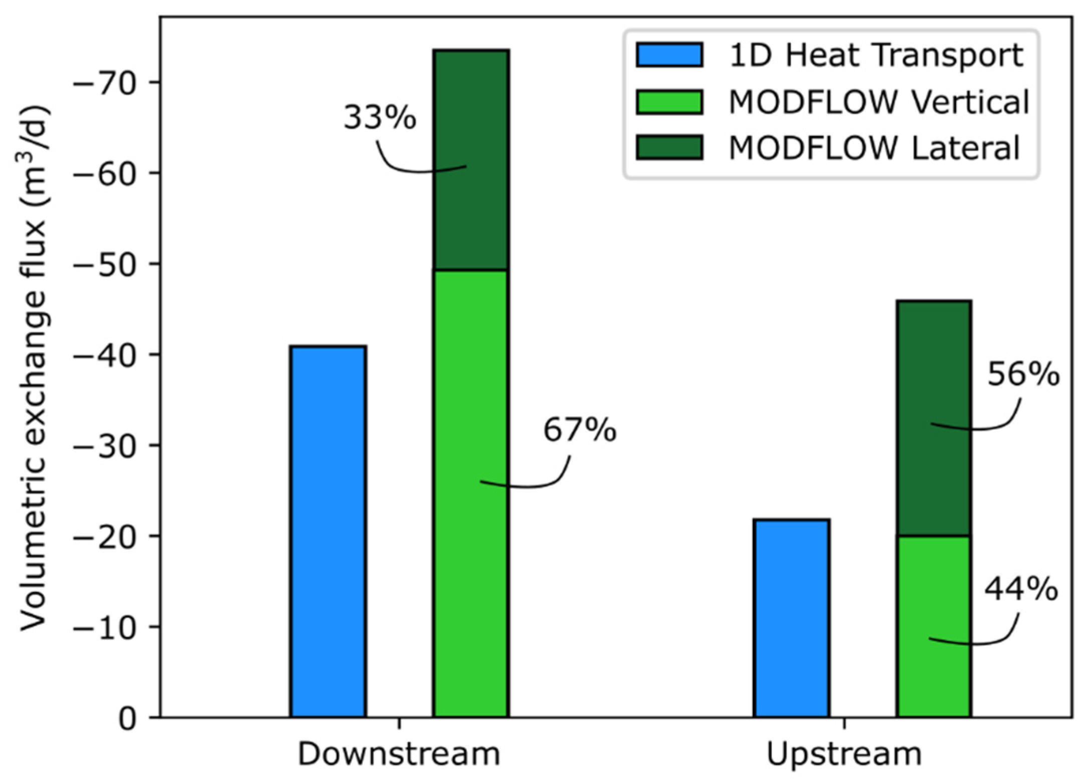
4.3. Comparison of Flux Estimates from Heat Transport and Groundwater Flow Modelling
4.4. Limitations
4.4.1. 1D Analytical Heat Tracer Method
4.4.2. 3D Numerical Groundwater Flow Model
5. Conclusions
Author Contributions
Funding
Institutional Review Board Statement
Informed Consent Statement
Data Availability Statement
Acknowledgments
Conflicts of Interest
References
- Brunner, P.; Therrien, R.; Renard, P.; Simmons, C.T.; Franssen, H.-J.H. Advances in understanding river-groundwater interactions. Rev. Geophys. 2017, 55, 818–854. [Google Scholar] [CrossRef]
- Conant, B.; Robinson, C.E.; Hinton, M.J.; Russell, H.A.J. A framework for conceptualizing groundwater-surface water interactions and identifying potential impacts on water quality, water quantity, and ecosystems. J. Hydrol. 2019, 574, 609–627. [Google Scholar] [CrossRef]
- Weatherill, J.J.; Atashgahi, S.; Schneidewind, U.; Krause, S.; Ullah, S.; Cassidy, N.; Rivett, M.O. Natural attenuation of chlorinated ethenes in hyporheic zones: A review of key biogeochemical processes and in-situ transformation potential. Water Res. 2018, 128, 362–382. [Google Scholar] [CrossRef] [PubMed] [Green Version]
- Kalbus, E.; Reinstorf, F.; Schirmer, M. Measuring methods for groundwater—Surface water interactions: A review. Hydrol. Earth Syst. Sci. 2006, 10, 873–887. [Google Scholar] [CrossRef] [Green Version]
- Rosenberry, D.O.; LaBaugh, J.W. Field Techniques for Estimating Water Fluxes between Surface Water and Ground Water; 4-D2; Geological Survey: Washington, DC, USA, 2008; p. 128.
- Gonzalez-Pinzon, R.; Ward, A.S.; Hatch, C.E.; Wlostowski, A.N.; Singha, K.; Gooseff, M.N.; Haggerty, R.; Harvey, J.W.; Cirpka, O.A.; Brock, J.T. A field comparison of multiple techniques to quantify groundwater–surface-water interactions. Freshw. Sci. 2015, 34, 139–160. [Google Scholar] [CrossRef] [Green Version]
- Baxter, C.; Hauer, F.R.; Woessner, W.W. Measuring Groundwater–Stream Water Exchange: New Techniques for Installing Minipiezometers and Estimating Hydraulic Conductivity. Trans. Am. Fish. Soc. 2003, 132, 493–502. [Google Scholar] [CrossRef]
- Cey, E.E.; Rudolph, D.L.; Parkin, G.W.; Aravena, R. Quantifying groundwater discharge to a small perennial stream in southern Ontario, Canada. J. Hydrol. 1998, 210, 21–37. [Google Scholar] [CrossRef]
- Conant, B., Jr. Delineating and quantifying ground water discharge zones using streambed temperatures. Ground Water 2004, 42, 243–257. [Google Scholar] [CrossRef]
- Darcy, H.P.G. Les Fountaines Publiques de la Ville de Dijon; Victor Dalmont: Paris, France, 1856; p. 647. [Google Scholar]
- Boano, F.; Harvey, J.W.; Marion, A.; Packman, A.I.; Revelli, R.; Ridolfi, L.; Wörman, A. Hyporheic flow and transport processes: Mechanisms, models, and biogeochemical implications. Rev. Geophys. 2014, 52, 2012RG000417. [Google Scholar] [CrossRef]
- Buss, S.R.; Cai, Z.; Cardenas, M.B.; Fleckenstein, J.H.; Hannah, D.M.; Heppell, K.; Hulme, P.J.; Ibrahim, T.; Kaeser, D.; Krause, S.; et al. The Hyporheic Handbook—A Handbook on the Groundwater-Surface Water Interface and Hyporheic Zone for Environmental Managers; SC050070; Environment Agency: Bristol, UK, 2009; p. 280.
- Cook, P.G. Estimating groundwater discharge to rivers from river chemistry surveys. Hydrol. Process. 2013, 27, 3694–3707. [Google Scholar] [CrossRef]
- Cox, M.H.; Su, G.W.; Constantz, J. Heat, Chloride, and Specific Conductance as Ground Water Tracers near Streams. Ground Water 2007, 45, 187–195. [Google Scholar] [CrossRef] [PubMed]
- Irvine, D.J.; Briggs, M.A.; Lautz, L.K.; Gordon, R.P.; McKenzie, J.M.; Cartwright, I. Using Diurnal Temperature Signals to Infer Vertical Groundwater-Surface Water Exchange. Ground Water 2016. [Google Scholar] [CrossRef] [PubMed]
- Rau, G.C.; Andersen, M.S.; McCallum, A.M.; Roshan, H.; Acworth, R.I. Heat as a tracer to quantify water flow in near-surface sediments. Earth-Sci. Rev. 2014, 129, 40–58. [Google Scholar] [CrossRef] [Green Version]
- Kurylyk, B.L.; Irvine, D.J.; Bense, V.F. Theory, tools, and multidisciplinary applications for tracing groundwater fluxes from temperature profiles. Wiley Interdiscip. Rev. Water 2019, 6, e1329. [Google Scholar] [CrossRef] [Green Version]
- Schmidt, C.; Conant, B.; Bayer-Raich, M.; Schirmer, M. Evaluation and field-scale application of an analytical method to quantify groundwater discharge using mapped streambed temperatures. J. Hydrol. 2007, 347, 292–307. [Google Scholar] [CrossRef]
- Anderson, M.P. Heat as a ground water tracer. Ground Water 2005, 43, 951–968. [Google Scholar] [CrossRef]
- Constantz, J. Heat as a tracer to determine streambed water exchanges. Water Resour. Res. 2008, 44. [Google Scholar] [CrossRef]
- Anibas, C.; Buis, K.; Verhoeven, R.; Meire, P.; Batelaan, O. A simple thermal mapping method for seasonal spatial patterns of groundwater–surface water interaction. J. Hydrol. 2011, 397, 93–104. [Google Scholar] [CrossRef]
- Jensen, J.K.; Engesgaard, P. Nonuniform Groundwater Discharge across a Streambed: Heat as a Tracer. Vadose Zone J. 2011, 10, 98–109. [Google Scholar] [CrossRef]
- Lewandowski, J.; Putschew, A.; Schwesig, D.; Neumann, C.; Radke, M. Fate of organic micropollutants in the hyporheic zone of a eutrophic lowland stream: Results of a preliminary field study. Sci. Total Environ. 2011, 409, 1824–1835. [Google Scholar] [CrossRef]
- Anibas, C.; Schneidewind, U.; Vandersteen, G.; Joris, I.; Seuntjens, P.; Batelaan, O. From streambed temperature measurements to spatial-temporal flux quantification: Using the LPML method to study groundwater-surface water interaction. Hydrol. Process. 2016, 30, 203–216. [Google Scholar] [CrossRef]
- Briggs, M.A.; Lautz, L.K.; Buckley, S.F.; Lane, J.W. Practical limitations on the use of diurnal temperature signals to quantify groundwater upwelling. J. Hydrol. 2014, 519, 1739–1751. [Google Scholar] [CrossRef]
- Rosenberry, D.O.; Briggs, M.A.; Delin, G.; Hare, D.K. Combined use of thermal methods and seepage meters to efficiently locate, quantify, and monitor focused groundwater discharge to a sand-bed stream. Water Resour. Res. 2016, 52, 4486–4503. [Google Scholar] [CrossRef] [Green Version]
- Bravo, H.R.; Jiang, F.; Hunt, R.J. Using groundwater temperature data to constrain parameter estimation in a groundwater flow model of a wetland system. Water Resour. Res. 2002, 38. [Google Scholar] [CrossRef]
- Karan, S.; Engesgaard, P.; Rasmussen, J. Dynamic streambed fluxes during rainfall- runoff events. Water Resour. Res. 2014, 50, 2293–2311. [Google Scholar] [CrossRef]
- Munz, M.; Oswald, S.E.; Schmidt, C. Coupled Long-Term Simulation of Reach-Scale Water and Heat Fluxes Across the River-Groundwater Interface for Retrieving Hyporheic Residence Times and Temperature Dynamics. Water Resour. Res. 2017, 53, 8900–8924. [Google Scholar] [CrossRef]
- Shope, C.L.; Constantz, J.E.; Cooper, C.A.; Reeves, D.M.; Pohll, G.; McKay, W.A. Influence of a large fluvial island, streambed, and stream bank on surface water-groundwater fluxes and water table dynamics. Water Resour. Res. 2012, 48, W06512. [Google Scholar] [CrossRef] [Green Version]
- Bredehoeft, J.D.; Papadopulos, I.S. Rates of vertical ground-water movement estimated from the Earth’s thermal profile. Water Resour. Res. 1965, 1, 325–328. [Google Scholar] [CrossRef]
- Turcotte, D.L.; Schubert, G. Geodynamics: Applications of Continuum Physics to Geological Problems; John Wiley & Sons: New York, NY, USA, 1982. [Google Scholar]
- Hatch, C.E.; Fisher, A.T.; Revenaugh, J.S.; Constantz, J.; Ruehl, C. Quantifying surface water-groundwater interactions using time series analysis of streambed thermal records: Method development. Water Resour. Res. 2006, 42. [Google Scholar] [CrossRef] [Green Version]
- Keery, J.; Binley, A.; Crook, N.; Smith, J.W.N. Temporal and spatial variability of groundwater-surface water fluxes: Development and application of an analytical method using temperature time series. J. Hydrol. 2007, 336, 1–16. [Google Scholar] [CrossRef]
- Luce, C.H.; Tonina, D.; Gariglio, F.; Applebee, R. Solutions for the diurnally forced advection-diffusion equation to estimate bulk fluid velocity and diffusivity in streambeds from temperature time series. Water Resour. Res. 2013, 49, 488–506. [Google Scholar] [CrossRef] [Green Version]
- Schneidewind, U. Water Flow and Contaminant Transformation in the Hyporheic Zone of Lowland Rivers. Ph.D. Thesis, Ghent University, Gent, Belgium, January 2016. [Google Scholar]
- Vandersteen, G.; Schneidewind, U.; Anibas, C.; Schmidt, C.; Seuntjens, P.; Batelaan, O. Determining groundwater-surface water exchange from temperature-time series: Combining a local polynomial method with a maximum likelihood estimator. Water Resour. Res. 2015, 51, 922–939. [Google Scholar] [CrossRef]
- Gordon, R.P.; Lautz, L.K.; Briggs, M.A.; McKenzie, J.M. Automated calculation of vertical pore-water flux from field temperature time series using the VFLUX method and computer program. J. Hydrol. 2012, 420, 142–158. [Google Scholar] [CrossRef]
- Irvine, D.J.; Lautz, L.K.; Briggs, M.A.; Gordon, R.P.; McKenzie, J.M. Experimental evaluation of the applicability of phase, amplitude, and combined methods to determine water flux and thermal diffusivity from temperature time series using VFLUX 2. J. Hydrol. 2015, 531, 728–737. [Google Scholar] [CrossRef] [Green Version]
- Swanson, T.E.; Cardenas, M.B. Ex-Stream: A MATLAB program for calculating fluid flux through sediment-water interfaces based on steady and transient temperature profiles. Comput. Geosci. 2011, 37, 1664–1669. [Google Scholar] [CrossRef]
- Van Berkel, M.; Vandersteen, G.; Schneidewind, U.; Anibas, A. LPML and LPMLE3 Codes: Local Polynomial Maximum Likelihood Estimator (Semi-Infinite and 3 Point); 4TU.Center for Research Data, Ed.; 4TU.Centre for Research Data: Delft, The Netherlands, 2018. [Google Scholar]
- Schornberg, C.; Schmidt, C.; Kalbus, E.; Fleckenstein, J.H. Simulating the effects of geologic heterogeneity and transient boundary conditions on streambed temperatures—Implications for temperature-based water flux calculations. Adv. Water Resour. 2010, 33, 1309–1319. [Google Scholar] [CrossRef]
- Cuthbert, M.O.; Mackay, R. Impacts of nonuniform flow on estimates of vertical streambed flux. Water Resour. Res. 2013, 49, 19–28. [Google Scholar] [CrossRef]
- Lautz, L.K. Impacts of nonideal field conditions on vertical water velocity estimates from streambed temperature time series. Water Resour. Res. 2010, 46. [Google Scholar] [CrossRef]
- Reeves, J.; Hatch, C.E. Impacts of three-dimensional nonuniform flow on quantification of groundwater-surface water interactions using heat as a tracer. Water Resour. Res. 2016, 52, 6851–6866. [Google Scholar] [CrossRef]
- Cranswick, R.H.; Cook, P.G.; Shanafield, M.; Lamontagne, S. The vertical variability of hyporheic fluxes inferred from riverbed temperature data. Water Resour. Res. 2014, 50, 3994–4010. [Google Scholar] [CrossRef]
- Shanafield, M.; Pohll, G.; Susfalk, R. Use of heat-based vertical fluxes to approximate total flux in simple channels. Water Resour. Res. 2010, 46. [Google Scholar] [CrossRef]
- Roshan, H.; Rau, G.C.; Andersen, M.S.; Acworth, I.R. Use of heat as tracer to quantify vertical streambed flow in a two-dimensional flow field. Water Resour. Res. 2012, 48. [Google Scholar] [CrossRef]
- Irvine, D.J.; Cranswick, R.H.; Simmons, C.T.; Shanafield, M.A.; Lautz, L.K. The effect of streambed heterogeneity on groundwater-surface water exchange fluxes inferred from temperature time series. Water Resour. Res. 2015, 51, 198–212. [Google Scholar] [CrossRef]
- Genereux, D.P.; Leahy, S.; Mitasova, H.; Kennedy, C.D.; Corbett, D.R. Spatial and temporal variability of streambed hydraulic conductivity in West Bear Creek, North Carolina, USA. J. Hydrol. 2008, 358, 332–353. [Google Scholar] [CrossRef]
- Ghysels, G.; Benoit, S.; Awol, H.; Jensen, E.P.; Debele Tolche, A.; Anibas, C.; Huysmans, M. Characterization of meter-scale spatial variability of riverbed hydraulic conductivity in a lowland river (Aa River, Belgium). J. Hydrol. 2018, 559, 1013–1027. [Google Scholar] [CrossRef]
- Zlotnik, V.; Tartakovsky, D.M. Interpretation of Heat-Pulse Tracer Tests for Characterization of Three-Dimensional Velocity Fields in Hyporheic Zone. Water Resour. Res. 2018, 54, 4028–4039. [Google Scholar] [CrossRef]
- Brunke, M.; Gonser, T. The ecological significance of exchange processes between rivers and groundwater. Freshw. Biol. 1997, 37, 1–33. [Google Scholar] [CrossRef] [Green Version]
- Kalbus, E.; Schmidt, C.; Bayer-Raich, M.; Leschik, S.; Reinstorf, F.; Balcke, G.U.; Schirmer, M. New methodology to investigate potential contaminant mass fluxes at the stream-aquifer interface by combining integral pumping tests and streambed temperatures. Environ. Pollut. 2007, 148, 808–816. [Google Scholar] [CrossRef]
- Woessner, W.W. Stream and fluvial plain ground water interactions: Rescaling hydrogeologic thought. Ground Water 2000, 38, 423–429. [Google Scholar] [CrossRef]
- Lautz, L.K.; Ribaudo, R.E. Scaling up point-in-space heat tracing of seepage flux using bed temperatures as a quantitative proxy. Hydrogeol. J. 2012, 20, 1223–1238. [Google Scholar] [CrossRef]
- Munz, M.; Oswald, S.E.; Schmidt, C. Analysis of riverbed temperatures to determine the geometry of subsurface water flow around in-stream geomorphological structures. J. Hydrol. 2016, 539, 74–87. [Google Scholar] [CrossRef]
- Ghysels, G.; Mutua, S.; Veliz, G.B.; Huysmans, M. A modified approach for modelling river–aquifer interaction of gaining rivers in MODFLOW, including riverbed heterogeneity and river bank seepage. Hydrogeol. J. 2019, 27, 1851–1863. [Google Scholar] [CrossRef]
- Kasahara, T.; Wondzell, S.M. Geomorphic controls on hyporheic exchange flow in mountain streams. Water Resour. Res. 2003, 39, 1–14. [Google Scholar] [CrossRef] [Green Version]
- Anibas, C.; Tolche, A.D.; Ghysels, G.; Nossent, J.; Schneidewind, U.; Huysmans, M.; Batelaan, O. Delineation of spatial-temporal patterns of groundwater/surface-water interaction along a river reach (Aa River, Belgium) with transient thermal modeling. Hydrogeol. J. 2018, 26, 819–835. [Google Scholar] [CrossRef]
- Anibas, C.; Fleckenstein, J.H.; Volze, N.; Buis, K.; Verhoeven, R.; Meire, P.; Batelaan, O. Transient or steady-state? Using vertical temperature profiles to quantify groundwater-surface water exchange. Hydrol. Process. 2009, 23, 2165–2177. [Google Scholar] [CrossRef]
- Baya Veliz, G. Influence of Riverbank Seepage on River-Aquifer Interactions at the Aa River. Master’s Thesis, Vrije Universiteit Brussel (VUB) & KU Leuven, Brussel, Belgium, 2017. [Google Scholar]
- Benoit, S.; Ghysels, G.; Gommers, K.; Hermans, T.; Nguyen, F.; Huysmans, M. Characterization of spatially variable riverbed hydraulic conductivity using electrical resistivity tomography and induced polarization. Hydrogeol. J. 2018, 27, 395–407. [Google Scholar] [CrossRef]
- Mohammed, G.A. Groundwater-Surface Water Interaction along a Lowland River. Ph.D. Thesis, Department of Hydrology and Hydraulic Engineering (HYDR), Vrije Universiteit Brussel (VUB), Brussel, Belgium, 2009. [Google Scholar]
- Mutua, S.M. Analysing the Influence of Groundwater-Surface Water Interaction on the Groundwater Balance in the Aa River. Master’s Thesis, Vrije Universiteit Brussel, Brussels, Belgium, 2013. [Google Scholar]
- Anibas, C.; Buis, K.; Getatchew, A.; Batelaan, O.; Verhoeven, R.; Meire, P. Determination of groundwater fluxes in the Belgian Aa River by sensing and simulation of streambed temperatures. In Proceedings of the Groundwater-Surface Water Interaction: Process Understanding, Conceptualization and Modelling—IUGG2007, Perugia, Italy, 2–13 July 2007; pp. 46–53. [Google Scholar]
- Dams, J.; Nossent, J.; Senbeta, T.B.; Willems, P.; Batelaan, O. Multi-modal approach to assess the impact of climate change on runoff. J. Hydrol. 2015, 529, 1601–1616. [Google Scholar] [CrossRef]
- RMI. Royal Meteorological Institute of Belgium [WWW Document]. Available online: https://www.meteo.be (accessed on 15 October 2019).
- Louwye, S.; De Schepper, S.; Laga, P.; Vandenberghe, N. The Upper Miocene of the southern North Sea Basin (northern Belgium): A palaeoenvironmental and stratigraphical reconstruction using dinoflagellate cysts. Geol. Mag. 2006, 144, 33–52. [Google Scholar] [CrossRef]
- Vandenberghe, N.; Harris, W.B.; Wampler, J.M.; Houthuys, R.; Louwye, S.; Adriaens, R.; Vos, K.; Lanckacker, T.; Matthijs, J.; Deckers, J.; et al. The implications of K-Ar glauconite dating of the Diest Formation on the paleogeography of the Upper Miocene in Belgium. Geol. Belg. 2014, 17, 161–174. [Google Scholar]
- DOV. Databank Ondergrond Vlaanderen. Available online: https://dov.vlaanderen.be/ (accessed on 14 October 2018).
- Chen, X.H. Measurement of streambed hydraulic conductivity and its anisotropy. Environ. Geol. 2000, 39, 1317–1324. [Google Scholar] [CrossRef]
- Stallman, R.W. Steady one-dimensional fluid flow in a semi-infinite porous medium with sinusoidal surface temperature. J. Geophys. Res. 1965, 70, 2821–2827. [Google Scholar] [CrossRef]
- Suzuki, S. Percolation Measurements Based on Heat Flow through Soil with Special Reference to Paddy Fields. J. Geophys. Res. 1960, 65, 2883–2885. [Google Scholar] [CrossRef]
- Irvine, D.J.; Kurylyk, B.L.; Briggs, M.A. Quantitative guidance for efficient vertical flow measurements at the sediment–water interface using temperature–depth profiles. Hydrol. Process. 2019, 34, 649–661. [Google Scholar] [CrossRef]
- Schmidt, C.; Bayer-Raich, M.; Schirmer, M. Characterization of spatial heterogeneity of groundwater-stream water interactions using multiple depth streambed temperature measurements at the reach scale. Hydrol. Earth Syst. Sci. 2006, 10, 849–859. [Google Scholar] [CrossRef] [Green Version]
- Bhaskar, A.S.; Harvey, J.W.; Henry, E.J. Resolving hyporheic and groundwater components of streambed water flux using heat as a tracer. Water Resour. Res. 2012, 48. [Google Scholar] [CrossRef]
- Arriaga, M.A.; Leap, D.I. Using solver to determine vertical groundwater velocities by temperature variations, Purdue University, Indiana, USA. Hydrogeol. J. 2004, 14, 253–263. [Google Scholar] [CrossRef]
- Deutsch, C.V.; Journel, A.G. GSLIB: Geostatistical Software Library and User’s Guide, 2nd ed.; Oxford University Press: Oxford, UK, 1998. [Google Scholar]
- Gringarten, E.; Deutsch, C.V. Teacher’s Aide Variogram Interpretation and Modeling. Math. Geol. 2001, 33, 507–534. [Google Scholar] [CrossRef]
- Remy, N.; Boucher, A.; Wu, J. Applied Geostatistics with SGeMS: A User’s Guide; Cambridge University Press: Cambridge, UK, 2009. [Google Scholar]
- Batelaan, O.; De Smedt, F. WetSpass: A flexible GIS based, distributed recharge methodology for regional groundwater modelling. In Proceedings of the Impact of Human Activity on Groundwater Dynamics at the 6th IAHS Scientific Assembly, Maastricht, The Netherlands, 18–21 July 2001; pp. 11–17. [Google Scholar]
- Bakker, M.; Post, V.; Langevin, C.D.; Hughes, J.D.; White, J.T.; Starn, J.J.; Fienen, M.N. Scripting MODFLOW Model Development Using Python and FloPy. Ground Water 2016, 54, 733–739. [Google Scholar] [CrossRef] [PubMed]
- Harbaugh, A.W. MODFLOW-2005, The U.S. Geological Survey Modular Ground-Water Model—The Ground-Water Flow Process; U.S. Geological Survey: Reston, VA, USA, 2005; p. 253.
- Freeze, R.A.; Cherry, J.A. Groundwater; Prentice-Hall: Englewood Cliffs, NJ, USA, 1979; p. 604. [Google Scholar]
- Storey, R.G.; Howard, K.W.F.; Williams, D.D. Factors controlling riffle-scale hyporheic exchange flows and their seasonal changes in a gaining stream: A three-dimensional groundwater flow model. Water Resour. Res. 2003, 39. [Google Scholar] [CrossRef]
- Sebok, E.; Duque, C.; Engesgaard, P.; Boegh, E. Spatial variability in streambed hydraulic conductivity of contrasting stream morphologies: Channel bend and straight channel. Hydrol. Process. 2015, 29, 458–472. [Google Scholar] [CrossRef]
- Schneidewind, U.; van Berkel, M.; Anibas, C.; Vandersteen, G.; Schmidt, C.; Joris, I.; Seuntjens, P.; Batelaan, O.; Zwart, H.J. LPMLE3: A novel 1-D approach to study water flow in streambeds using heat as a tracer. Water Resour. Res. 2016, 52, 6596–6610. [Google Scholar] [CrossRef] [Green Version]
- Shanafield, M.; Hatch, C.; Pohll, G. Uncertainty in thermal time series analysis estimates of streambed water flux. Water Resour. Res. 2011, 47. [Google Scholar] [CrossRef]
- Hopmans, J.W.; Simunek, J.; Bristow, K.L. Indirect estimation of soil thermal properties and water flux using heat pulse probe measurements: Geometry and dispersion effects. Water Resour. Res. 2002, 38, 7-1–7-14. [Google Scholar] [CrossRef]
- Sebok, E.; Müller, S. The effect of sediment thermal conductivity on vertical groundwater flux estimates. Hydrol. Earth Syst. Sci. 2019, 23, 3305–3317. [Google Scholar] [CrossRef] [Green Version]
- Soto-López, C.D.; Meixner, T.; Ferré, T.P.A. Effects of measurement resolution on the analysis of temperature time series for stream-aquifer flux estimation. Water Resour. Res. 2011, 47, W12602. [Google Scholar] [CrossRef] [Green Version]
- Banks, E.W.; Shanafield, M.A.; Noorduijn, S.; McCallum, J.; Lewandowski, J.; Batelaan, O. Active heat pulse sensing of 3-D-flow fields in streambeds. Hydrol. Earth Syst. Sci. 2018, 22, 1917–1929. [Google Scholar] [CrossRef] [Green Version]
- Angermann, L.; Krause, S.; Lewandowski, J. Application of heat pulse injections for investigating shallow hyporheic flow in a lowland river. Water Resour. Res. 2012, 48, W00P02. [Google Scholar] [CrossRef] [Green Version]
- Gómez-Hernández, J.J.; Wen, X.-H. To be or not to be multi-Gaussian? A reflection on stochastic hydrogeology. Adv. Water Resour. 1998, 21, 47–61. [Google Scholar] [CrossRef]
- Mustafa, S.M.T.; Nossent, J.; Ghysels, G.; Huysmans, M. Integrated Bayesian Multi-model approach to quantify input, parameter and conceptual model structure uncertainty in groundwater modeling. Environ. Model. Softw. 2020, 126, 104654. [Google Scholar] [CrossRef]


| Parameter | Value | Unit |
|---|---|---|
| Thermal conductivity k | 1.8 | J/(s·m·K) |
| 1000 | kg/m3 | |
| 4183 | J/(kg·K) | |
| Variable | °C | |
| 11.2 | °C |
| Section | Direction | Nugget (mm²/day²) | Sill (mm²/day²) | Range (m) |
|---|---|---|---|---|
| Downstream | Omni | 0 | 1900 | 8 |
| Along | 0 | 1600 | 8 | |
| Across | 0 | 2200 | 8 | |
| Upstream | Omni | 0 | 1100 | 8 |
| Along | 0 | 1100 | 11 | |
| Across | 0 | 1100 | 6.5 |
| Section | Method | Avg. (mm/day) | Median (mm/day) | Min. (mm/day) | Max. (mm/day) | St. Dev. (mm/day) |
|---|---|---|---|---|---|---|
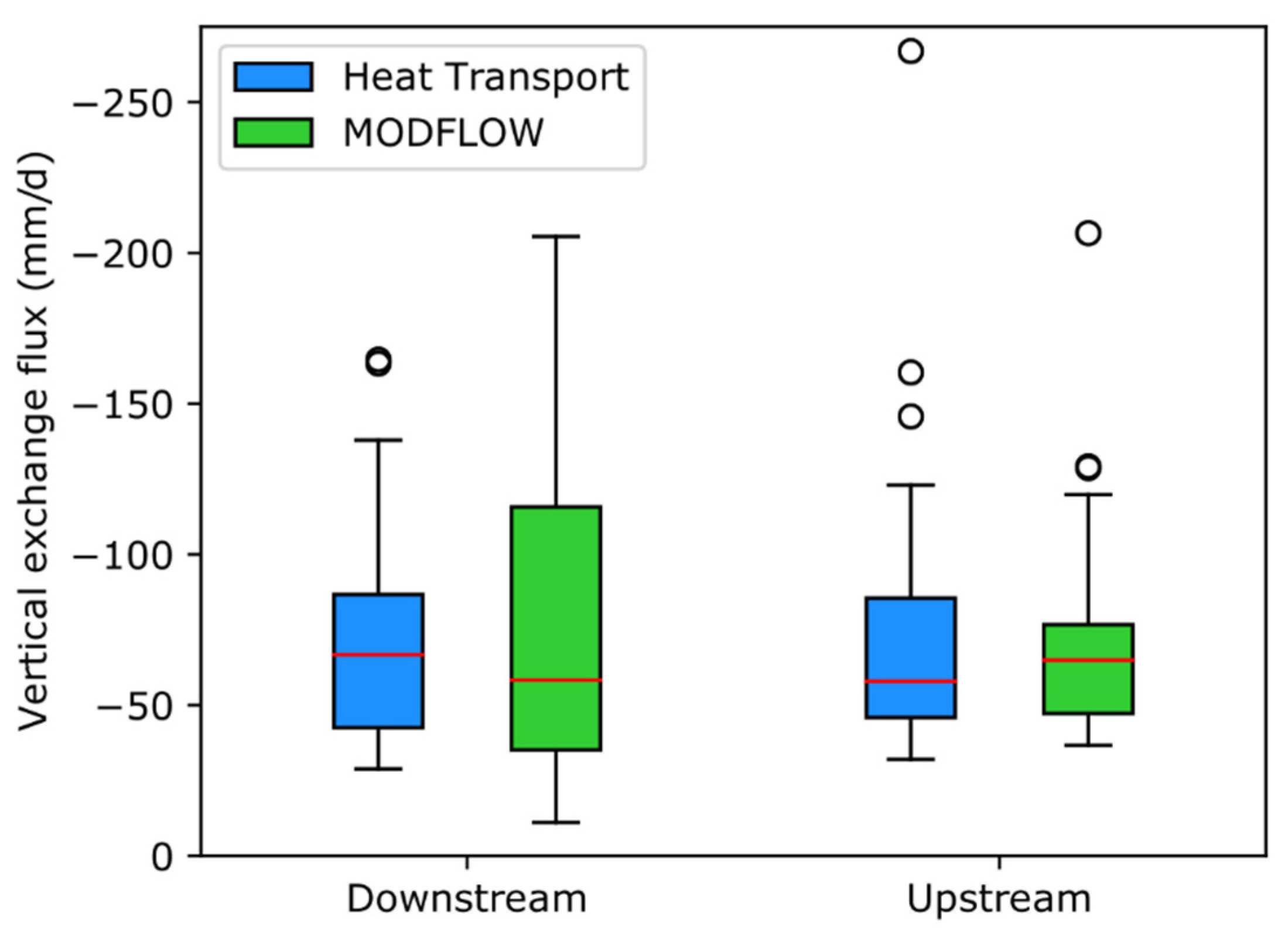
| Downstream | Heat Transport | −72.5 | −57.9 | −32.0 | −266.9 | 41.4 |
| MODFLOW | −68.8 | −64.9 | −36.7 | −206.5 | 31.2 | |
| Upstream | Heat Transport | −69.4 | −66.7 | −28.9 | −164.6 | 30.9 |
| MODFLOW | −76.7 | −58.3 | −11.1 | −205.5 | 54.1 |
Publisher’s Note: MDPI stays neutral with regard to jurisdictional claims in published maps and institutional affiliations. |
© 2021 by the authors. Licensee MDPI, Basel, Switzerland. This article is an open access article distributed under the terms and conditions of the Creative Commons Attribution (CC BY) license (http://creativecommons.org/licenses/by/4.0/).
Share and Cite
Ghysels, G.; Anibas, C.; Awol, H.; Tolche, A.D.; Schneidewind, U.; Huysmans, M. The Significance of Vertical and Lateral Groundwater–Surface Water Exchange Fluxes in Riverbeds and Riverbanks: Comparing 1D Analytical Flux Estimates with 3D Groundwater Modelling. Water 2021, 13, 306. https://doi.org/10.3390/w13030306
Ghysels G, Anibas C, Awol H, Tolche AD, Schneidewind U, Huysmans M. The Significance of Vertical and Lateral Groundwater–Surface Water Exchange Fluxes in Riverbeds and Riverbanks: Comparing 1D Analytical Flux Estimates with 3D Groundwater Modelling. Water. 2021; 13(3):306. https://doi.org/10.3390/w13030306
Chicago/Turabian StyleGhysels, Gert, Christian Anibas, Henock Awol, Abebe Debele Tolche, Uwe Schneidewind, and Marijke Huysmans. 2021. "The Significance of Vertical and Lateral Groundwater–Surface Water Exchange Fluxes in Riverbeds and Riverbanks: Comparing 1D Analytical Flux Estimates with 3D Groundwater Modelling" Water 13, no. 3: 306. https://doi.org/10.3390/w13030306