
Water Demand Prediction Using Machine Learning Methods: A Case Study of the Beijing–Tianjin–Hebei Region in China


Department of Construction Management, School of Economics and Management, Beijing Jiaotong University, Beijing 100044, China
*
Author to whom correspondence should be addressed.
Water 2021, 13(3), 310; https://doi.org/10.3390/w13030310
Submission received: 15 December 2020
/
Revised: 19 January 2021
/
Accepted: 22 January 2021
/
Published: 27 January 2021
(This article belongs to the Section Urban Water Management)
Abstract
:Predicting water demand helps decision-makers allocate regional water resources efficiently, thereby preventing water waste and shortage. The aim of this study is to predict water demand in the Beijing–Tianjin–Hebei region of North China. The explanatory variables associated with economy, community, water use, and resource availability were identified. Eleven statistical and machine learning models were built, which used data covering the 2004–2019 period. Interpolation and extrapolation scenarios were conducted to find the most suitable predictive model. The results suggest that the gradient boosting decision tree (GBDT) model demonstrates the best prediction performance in the two scenarios. The model was further tested for three other regions in China, and its robustness was validated. The water demand in 2020–2021 was provided. The results show that the identified explanatory variables were effective in water demand prediction. The machine learning models outperformed the statistical models, with the ensemble models being superior to the single predictor models. The best predictive model can also be applied to other regions to help forecast water demand to ensure sustainable water resource management.
1. Introduction
Water scarcity is an issue for many cities globally [1]. By 2030, nearly half of the world’s population is expected to live in water-stressed areas [2]. Water demand prediction is crucial for the sustainable management of water distribution systems [3]. It is also a factor that is considered by infrastructure decision-makers to ensure effective water usage plans and schedules, especially in light of the ongoing urban expansion, where consumers are encouraged to reduce their energy and resource consumption [4,5,6].
The economy of the Beijing–Tianjin–Hebei region has been developing rapidly. The demand for city expansion from Beijing to Tianjin and Hebei has increased. This rapid urban expansion has tightened the region’s ability to provide adequate water resources. In the existing water distribution conditions, regional water resource management faces uncertainties and challenges such as water shortages, overall growth in water demand, seasonal demand peaks due to climate change, regional economic competition, and public health requirements.
This study focuses on water demand prediction in the Beijing–Tianjin–Hebei region to support water resource planning and management. The explanatory variables associated with economy, community, water use, and resource availability were derived. A historical dataset covering the period from 2004 to 2019 was collected from the Annual Water Resources Reports [7,8,9] and China Statistics Yearbook [10]. Eleven prediction models, containing both statistical and machine learning models, were designed. Two prediction scenarios were considered. In the interpolation prediction scenario (IPS), the training and the test samples were randomly selected from the entire dataset. In the extrapolation prediction scenario (EPS), the historical dataset was used for training to predict the future water demand. Their performances were compared to identify the most suitable model. To prove its robustness, the best model was further tested on three other regions in China with different geography, climates, and economies. Further, we predicted the water demand for the next two years. The results of this study will help water utilities and policymakers recognize the water demand situation in the Beijing–Tianjin–Hebei region, helping them to formulate water resource management policies effectively and to ensure a stable long-term water supply.
2. Literature Review
A prediction model combines economic and social factors with geographic information to forecast water demand. There are two main steps used in prediction modeling: explanatory variables selection and model building. Explanatory variables (or model features) are selected based on their ability to explain trends in water demand. The model building process involves applying an algorithm to learn the relationship between the selected features and the prediction target (water demand in this case).
2.1. Variables Considered in the Literature for Explaining Water Demand
Studies have shown that urban water demand is impacted by many factors, including economy, society, climate, and environment. Lu et al. [11] developed a hybrid model for predicting monthly water demand in Austin, Texas, pointing out that the demand was highly related to the local population, monthly average temperature, and monthly average humidity. Li et al. [12] used principal component analysis regression to study the annual water demand in Shanghai; the authors found that the population and gross domestic product (GDP) have a significant impact on annual water demand. Zhao and Chen [13] adopted the elastic back propagation neural network algorithm to predict the water demand of urban residents using features such as per capita GDP, the quality of the population (level of education), water prices, temperature, water companies’ total annual water supply, and seasonal changes. Tian and Xue [14] built a backpropagation (BP) neural network model for predicting annual water consumption in Guangdong, China, using features such as total water resources, precipitation, GDP, industrial added value, permanent residents, added value of tertiary industry, effective irrigated area, added value of agriculture, forestry, animal husbandry and fishery, and urban green area. Zhang et al. [15] built models for analyzing water demand in Beijing and Jinan, China, considering factors such as population, GDP, added value in primary, secondary, and tertiary industries, and per capita water resources. Sun et al. [16] evaluated the sustainable use of water resources in Beijing, China, considering the factors of economy, population, water supply and demand, land resources, and water pollution and management. Tang et al. [17] proposed an improved BP neural network model for predicting water demand in Hubei, Chia, using features such as population, farmland irrigation area, GDP, and industrial added value. Zhang et al. [18] found that regional GDP, agricultural output value, industrial output value, year-end population, irrigation area, and per capita disposable income were related to regional water demand. Wang et al. [19] chose population, gross agricultural production, and gross industrial production as the main factors affecting annual water demand in Nanchang city, China. Water demand was also found to be related to climatic factors such as precipitation [20,21]. Table 1 summarizes the explanatory variables affecting water demand.

Table 1.
Main explanatory variables found by other studies to affect water demand.
| Explanatory variables | Unit | Lu et al. [11] | Li et al. [12] | Zhao and Chen [13] | Tian and Xue [14] | Zhang et al. [15] | Sun et al. [16] | Tang et al. [17] | Zhang et al. [18] | Wang et al. [19] | Tiwari et al. [20] | Chen et al. [21] | |
|---|---|---|---|---|---|---|---|---|---|---|---|---|---|
| Economy | GDP | Billion Yuan | √ | √ | √ | √ | √ | √ | |||||
| Per capita GDP | Yuan per Person | √ | √ | √ | |||||||||
| Added value of primary industry | Billion Yuan | √ | √ | √ | √ | ||||||||
| Added value of secondary industry | Billion Yuan | √ | √ | ||||||||||
| Added value of tertiary industry | Billion Yuan | √ | √ | √ | |||||||||
| Per capita disposable income | Yuan | √ | √ | √ | |||||||||
| Community | Year-end population | Million | √ | √ | √ | √ | √ | √ | √ | ||||
| Water use | Agricultural water consumption | Billion m3 | √ | √ | √ | ||||||||
| Irrigated area | Thousand Hectare | √ | √ | √ | √ | ||||||||
| Resource availability | Total water resources | Billion m3 | √ | ||||||||||
| Annual precipitation | mm | √ | √ | √ | |||||||||
2.2. Models for Predicting Water Demand
Choosing an appropriate water demand prediction model is a challenge because it involves many factors, such as technology, population, society, economy, climate, and public policy [3,22,23]. Predictive models can be broadly divided into two groups: statistical and machine-learning models. Statistical models employ probability theory and mathematical statistics to obtain the functional relationship between different variables. Commonly use statistical models for regression include linear regression, ridge regression, and lasso regression. In contrast, machine learning models do not require defining a clear relationship between dependent and explanatory variables [5,24]. Instead, they employ algorithms such as support vector machine, decision tree, and random forest to learn patterns from training data and use them to predict future outcomes.
Statistical models are widely used for water demand prediction [25,26,27,28]. The main limitation of statistical models is that they must have a predetermined structure [29], making it difficult to find one mathematical function that would work well on different data [30]. Furthermore, statistical models often fail to effectively deal with complex data relationships; their prediction accuracy also decreases with an increase in the amount of data [31]. Other methods should be employed when dealing with big and complex data [32]. For example, Rozos et al. [33] employed an integrated system dynamics and cellular automata model to predict water demand under alternative approaches, including distributed water infrastructure.
Machine learning models are becoming increasingly popular and have demonstrated high predictive performance in domains such as urban infrastructure [34,35,36,37], credit risk [38,39], energy [40], ecology [41,42,43], and water resource management [44].
Machine learning models can be further divided into single predictors and ensemble algorithms, according to the number of employed predictors. A single predictor contains only one predictor (or algorithm), such as neural network, support vector machine, or decision tree. Ensemble algorithms such as random forest, AdaBoost, bagging, and gradient-boosting tree aggregate a number of predictors, all contributing to the final prediction result.
Ensemble learning is becoming increasingly popular [45,46]. It uses statistical sampling principles to train multiple models. Each of these models is used to separately predict a new sample. The value of the final prediction result for the new sample is selected based on the majority voting mechanism. In other words, ensemble learning transforms different hypotheses provided by single predictors into one hypothesis.
In the field of predicting water resources, Lee et al. [30] investigated 12 statistical and machine-learning models to predict daily household water usage in response to residential water demand. Pesantez et al. [5] applied random forest, artificial neural network, and support vector machine to smart-meter data to predict the hourly water demand of 90 accounts. Parisouj et al. [47] employed support vector regression, artificial neural network with backpropagation, and extreme learning machine to predict the monthly and daily streamflows of four river basins in the United States. Villarin and Rodriguez-Galiano [32] used classification and regression trees and random forest to establish a multivariate prediction model for water demand in Seville, Spain. Sengupta et al. [48] used support vector machine, artificial neural network, and random forest to predict changes in stream channel morphology.
China’s Beijing–Tianjin–Hebei region is an area with a severe water shortage. Water demand prediction can help its decision-makers to achieve more efficient water resource allocation. Existing studies have used one or a few models to predict water demand. In contrast, this study provides, for the first time, a comprehensive comparative analysis of several statistical and machine-learning models under IPS and EPS. The training and test data refer to the same period of time under IPS, whereas models are built using historical training data and then applied to predict future water demand under EPS.
3. Methodology
3.1. Research Design
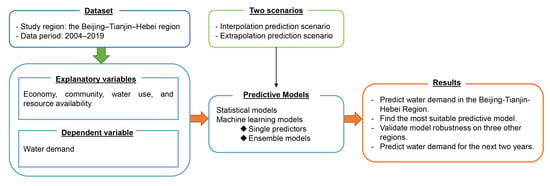
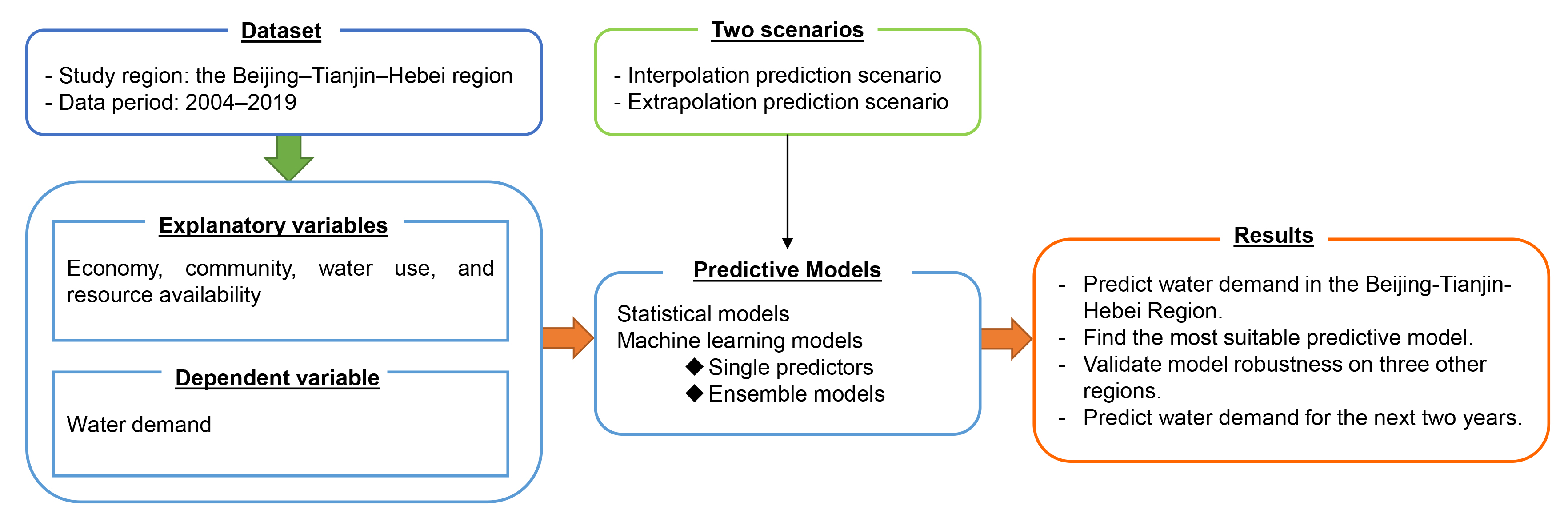
This study was designed to investigate the performance of 11 modeling techniques under two prediction scenarios of water demand in the Beijing–Tianjin–Hebei region. The research design was divided into five steps: data preprocessing, modeling, model training, cross-validation (CV), and model testing (Figure 1).
As the first step, data preprocessing allowed us to reduce the sensitivity of the models to different data scales. The following two prediction scenarios were considered (more details are provided in Section 3.4, Section 3.5 and Section 3.6):
- (1)
- Interpolation prediction scenario (IPS): For each model, a 10-fold CV was applied to randomly selected training samples accounting for 80% of all the data. The fitted models were then tested on the remaining 20% of the data to verify their prediction performance.
- (2)
- Extrapolation prediction scenario (EPS): For each model, a 10-fold CV was applied to the training data covering the period from 2004 to 2018. The fitted models were then tested on the 2019 data.
3.2. Data Preprocessing
Feature scaling was used consistently across all the studied models to ensure the comparability of their prediction results. Normalization was chosen as the feature scaling method. Let D = {X, y} denote the training set, where X = (x1, x2, …, xn) is the n-dimensional explanatory space, and y represents the dependent variable. The normalization of xi can be expressed as
where xi’ denotes the normalized value of an explanatory variable x for an ith sample; max(x) and min(x) denote the maximum and minimum values of x, respectively. Both explanatory and dependent variables were normalized in this study.
3.3. Modeling
The following 11 models were introduced in this study to predict water demand:
- Statistical models: linear regression (LR), ridge regression, least absolute shrinkage and selection operator (lasso) regression, kernel ridge regression (KRR), and Bayesian ridge regression (BRR);
- Machine learning models:
- ➢
- Single predictors: backpropagation neural network (BPNN), decision tree (DT), and support vector machine (SVM);
- ➢
- Ensemble methods: random forest (RF), adaptive boosting (AdaBoost), and gradient-boosting decision tree (GBDT). RF is a parallel integration algorithm, whereas AdaBoost and GBDT are serial-integration algorithms.
The Python Scikit-Learn library [49,50] was used to implement the models. The prediction models for each method listed in Section 3.3 were built separately. The default hyperparameter values of each algorithm were used to train the models. Each algorithm is briefly described below.
3.3.1. Linear Regression
LR expresses the relationship between the explanatory variable(s) x and the dependent variable y through a linear function. It fits a linear model to minimize the residual sum of squares between the actual and estimated values of the dependent variable. The coefficients are estimated using the ordinary least squares (OLS) method.
3.3.2. Ridge and Lasso Regression
Ridge regression and lasso regression are variations of LR. Ridge regression [51] is an improvement of the OLS method. It is a more stable and reliable regression algorithm, owing to the employment of the loss of unbiasedness [52]. The regularization term L2 is added after the sum of squared error (SSE) to control the trade-off between variance and bias.
Lasso regression was proposed by Tibshirani [53]. The important characteristic of this algorithm is that it completely eliminates the least important features by setting their weights to zero [52]. Lasso regression automatically performs feature selection and outputs a sparse matrix model. It replaces the regularization term L2 with the regularization term L1.
3.3.3. Kernel and Bayesian Ridge Regression
KRR is an extension of ridge regression that works well on nonlinear data by mapping them to a new feature space using a kernel, where the data become linearly separable. BRR combines ridge regression with Bayesian statistics.
3.3.4. Backpropagation Neural Network
BPNN, also known as a multilayer perceptron (MLP), comprises an input layer, one or more hidden layers, and an output layer. Its signal propagates forward from the input layer to the output layer through the hidden layers, while the error propagates backward from the output layer to the input layer [54].
In BPNN, a weight vector is applied element-wise to the input feature vector, and the result is passed through an activation function to obtain the dependent value. The commonly used activation functions are threshold, sigmoid, and hyperbolic tangent functions. The objective function is the SSE. The minimum value of the objective function is determined using the gradient descent method.
3.3.5. Decision Tree
DT is a classic machine-learning algorithm. It builds a binary tree based on sample features. The process of arriving at the prediction result is easy to understand and interpret since the resulting decision tree structure is similar to a flowchart, where leaf nodes correspond to the predicted values.
3.3.6. Support Vector Machine
SVM finds a separating hyperplane, fitting y based on x with the largest margin. SVM uses a kernel function to map the original training set with nonlinear features to a high-dimensional feature space, where the data become linearly separable [55]. The popular kernel functions are linear, polynomial, and radial basis functions.
3.3.7. Random Forest
RF, first proposed by Breiman [56], is an ensemble learning algorithm that uses the bagging algorithm for feature selection. In particular, replacement without sampling is used to randomly select a subset of features to construct each tree in the ensemble, while replacement sampling is used to select samples from the original data to train the trees. For each new test sample, the prediction result output by each trained tree in the ensemble is integrated using the majority voting mechanism to obtain the final result.
3.3.8. AdaBoost
AdaBoost is a famous boosting algorithm [57], where each sample is assigned an initial weight, and the weighted data set is then used to train a model. The weight of a sample is increased if the prediction result for it is wrong. Then, the next model is trained again by increasing some weights. This process is repeated several times to get weak learners. The weak learners are then combined to obtain a strong learner [58].
3.3.9. Gradient Boosting Decision Tree
GBDT, first developed by Friedman [59], uses gradient boosting to promote performance. It updates parameters in the direction of the gradient descent. The model’s performance is evaluated using a loss function. GBDT usually operates as a combination of decision trees. Each decision tree learns the residuals from all previous trees. The final result is the aggregation of the results obtained by all decision trees [60].
3.4. Model Training
Random samples, accounting for 80% of the entire dataset, covering the period from 2004 to 2019, constituted the training data in the IPS model. The training data in the EPS model were the data from 2004 to 2018.
3.5. Cross-Validation
When fitting a model using the training set and validating it using the test set, the model can be prone to overfitting, i.e., the model will perform well on seen data but poorly on unseen data. To overcome the problem of overfitting, a 10-fold CV was introduced for the training data. The 10-fold CV randomly divides the training data into ten different subsets, with each subset constituting one fold. Each model is then trained on the nine folds and validated on the remaining fold 10 times, with the validation fold changed in each iteration. The average prediction score and the standard deviation are calculated using the ten scores output by CV. The same CV process was adopted for both IPS and EPS.
3.6. Model Testing
The remaining random samples that account for 20% of the entire dataset for the period from 2004 to 2019 constituted the test data in the IPS model. The test data in the EPS model were the data for 2019 only. To evaluate each model’s performance, the following three metrics were employed: mean squared error (MSE), mean absolute error (MAE), and coefficient of determination (R2). These metrics were considered due to their wide use in studies on water demand prediction [5,30,31,32].
MSE and MAE were used to measure the difference between the actual and predicted values for each sample as follows:
where denotes the predicted value of the ith sample; yi denotes the corresponding actual value; n denotes the number of samples. Lower values of MSE and MAE indicate a better fit of models.
R2 indicates the goodness of fit. It measures the proportion of variance explained by the explanatory variables used in a model, as follows:
where and yi denote the predicted and corresponding actual values of the ith sample, respectively, and denotes the average value of all actual values, . The proportion of explained variance reflects how well unseen samples are predicted. The best possible value of R2 is 1.0.
4. Cast Study: Beijing–Tianjin–Hebei Region in China
4.1. Study Region
The Beijing–Tianjin–Hebei region is located in the north of China, comprising Beijing, Tianjin, and Hebei. It has a population of 110 million and covers an area of 21.67 million ha [61]. The Beijing–Tianjin–Hebei region is adjacent to China’s most water-short river basin. The region suffers serious water scarcity problems [61,62,63].
The total amount of water resources in the Beijing–Tianjin–Hebei region in 2019 was 14.62 billion m3 [10]. The per capita water resources of Beijing, Tianjin, and Hebei were 114.02, 51.79, and 149.5 m3 per person, respectively, which is far below the internationally recognized extreme water shortage standard of 500 m3 per person. While the total amount of water resources in the Beijing–Tianjin–Hebei region is less than 1% of the total water resources of the country, the region accounts for 8% of the country’s total GDP and population.
4.2. Dataset
The following eleven explanatory variables were chosen to characterize water demand based on the literature review presented in Section 2.1:
- Economy: GDP, per capita GDP, added value of primary industry, added value of secondary industry, added value of tertiary industry, and per capita disposable income;
- Community: year-end population;
- Water use: agriculture water consumption and irrigated area;
- Resource availability: total water resources and annual precipitation.
Agriculture water consumption and annual precipitation for the Beijing–Tianjin–Hebei region from 2004 to 2019 were obtained from the Annual Water Resources Reports [7,8,9], while the data from the same period for the remaining variables came from the China Statistics Yearbook [10]. The explanatory variable dataset had 48 rows and 16 columns, of which 48 represented 16 years of historical data from Beijing, Tianjin, and Hebei, and 11 represented the number of explanatory variables. The water demand of the Beijing–Tianjin–Hebei region is the sum of each subregion. Table A1 listed the basic statistics of the variables.
4.3. Predictive Results
4.3.1. Training and CV Results
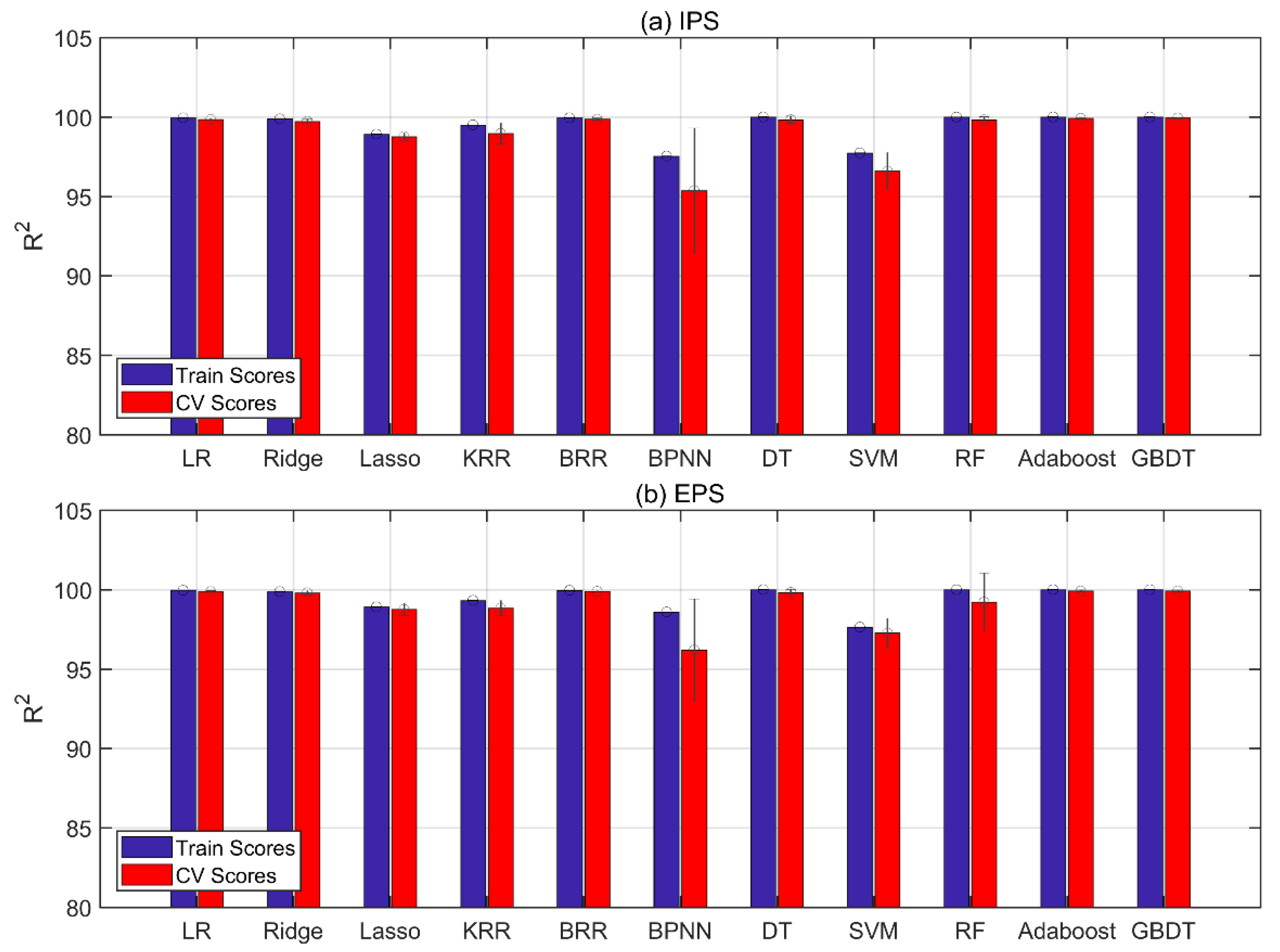
The blue and red bars in Figure 2 represent the training and CV R2 scores for all 11 models, respectively, with the black circles and lines representing the mean and standard deviation of the CV scores, respectively. LR was considered as the baseline model across all the statistical models.
The CV scores of all the models were higher than 95% in IPS. Relatively large standard deviations were observed for KRR, BPNN, and SVM, indicating that the R2 values were highly dispersed across the ten-folds of these models, which means that the models’ performance in each fold significantly deviated from the average performance. In addition to lower standard deviations, the CV scores of LR, BRR, AdaBoost, and GBDT models ranked in the top four. These four models were considered for the test set.
Similarly, the CV scores of all the models were also higher than 95% in EPS. Lasso, KRR, BPNN, SVM, and RF showed higher standard deviations in this scenario. The models that obtained the best CV performance were also the LR, BRR, AdaBoost, and GBDT models. These four models were further promoted to the test set.
The CV performance of the models in EPS was slightly lower than that in IPS. This was mainly because the EPS model focused on future prediction, for which it is much more difficult to achieve a higher prediction effect. On the contrary, IPS predicted data from the same historical period as the training data. Hence, the uncertainties were lower than that in the case of EPS.
4.3.2. Test Results
Table 2 shows the results achieved by the models over the test set under IPS and EPS, respectively. The best values for each metric are highlighted in bold.
The GBDT model outperformed the other models in both scenarios, achieving the lowest MSE and MAE and R2 scores of 99.9999% and 99.9578% in IPS and EPS, respectively. The R2 scores of LR, BRR, and AdaBoost models were lower than that of GBDT by 0.0531%, 0.0529%, and 0.0002%, respectively, in IPS; in EPS, AdaBoost came second and BRR and LR came third and fourth. The test results confirm that the machine-learning models outperform the statistical models, with the ensemble models being superior to the single predictor models. The best model for predicting water demand in these two scenarios is GBDT.
4.3.3. Model Robustness
The GBDT model was further applied to three other regions in China to verify its robustness because it exhibited the best performance in both IPS and EPS. However, the other three models (i.e., LR, BRR, and AdaBoost; see Table 2) had only slightly lower efficiencies. All four models were, therefore, tested for model robustness.
The Harbin–Changchun region is located in the northeast of China, and it comprises Heilongjiang and Jilin, covering an area of 263,640.92 km2 and having an estimated population of 65 million. The Central Plains urban region is located in the central and eastern parts of China and comprises Henan, Shanxi, Hebei, Shandong, and Anhui. It covers an area of 287,000 km2 and has an estimated population of 374 million. The Chengdu–Chongqing region is located in southwestern China and comprises Szechwan and Chongqing. It covers an area of 185,000 km2 and has a population of 115 million. These three regions have vastly different geographical locations (from the north to the south of China) and climate and economic conditions.
The yearly explanatory variables and the dependent variable were collected from 2004 to 2019, according to the related reports [64,65,66,67,68,69,70,71]. The dataset size was 32 × 11, 80 × 11, and 32 × 11 for the Harbin–Changchun region, the Central Plains urban region, and the Chengdu–Chongqing region, respectively. The explanatory variable data were imported into the LR, BRR, AdaBoost, and GBDT models to obtain the predicted value of annual water demand.
Figure 3 shows the comparison results of the actual and predicted values of water demand in the three regions. The LR model’s prediction results are not shown in Figure 3 because the model failed to obtain effective prediction results. This indicates that the LR model is effective for predicting the water demand in the Beijing–Tianjin–Hebei region but cannot be extended to other regions in China.
In contrast, BRR, AdaBoost, and GBDT models could predict the outcomes. The prediction accuracy (R2) of the GBDT model reached 93.1503% (Harbin–Changchun region), 83.1108% (Central Plains urban region), and 93.3015% (Chengdu–Chongqing region). It also obtained the highest prediction accuracy for the Central Plains urban region, with an accuracy greater than that of BRR and AdaBoost models by 8% and 35%, respectively. These models showed minor differences (i.e., the accuracy difference was less than 5%) for the Harbin–Changchun region and the Chengdu–Chongqing region. The BRR model achieved the best results, which was both 3% higher than the other two models for the Harbin–Changchun region and 2% and 3% higher than that of AdaBoost and GBDT models for the Chengdu–Chongqing region. The AdaBoost model performed poorly for the Central Plains urban region, with only 47.93% accuracy. The accuracy should be higher than 50% for robust and acceptable model performance [72,73]. Overall, the GBDT and BRR models proved to be robust. Compared with these two models, the accuracy of the GBDT model was better than that of the BRR model by 3% in these three regions.
Good agreement was not obtained for the Chengdu–Chongqing region before 2012. The early economic growth for this region was relatively flat. Its economic growth rate could not match the Beijing–Tianjin–Hebei region. Further, the region experienced a magnitude-8 earthquake in 2008. Its reconstruction was not completed until the end of 2011 [74]. To accelerate economic development, the Chengyu Economic Zone was established in May 2011. The construction of this economic zone has promoted regional economic development. As seen from Figure 3, the differences between the predicted and actual values decreased after 2012.
4.3.4. Prediction for the Next Two Years
Water demand in the Beijing–Tianjin–Hebei region for the next two years was further predicted. It is difficult to obtain the relevant explanatory variables in a timely manner and to use them to predict the next two years of water demand. Here, we adjusted the forecast period to predict the next two years of water demand.
The next two years’ prediction (NTYP) was similar to the EPS model. The EPS model was trained using the data of the past 15 years (i.e., 2004 to 2018) and was tested on the 16th year’s (i.e., 2019) water demand. NTYP was trained using the data of the past 12 years to predict the future 12 years’ water demand. The GBDT model was used in NTYP as it achieved the best performance in EPS. The actual and predicted values of water demand are shown in Figure 4.
The R2 scores from 2010 to 2019 were 86.62% (Beijing), 94.94% (Tianjin), and 95.57% (Hebei). The water demand in the Beijing–Tianjin–Hebei region was the sum of the demands of its subregions. For the next two years, Beijing’s water demand remains stable, while Tianjin’s water demand first decreases and then increases. Hebei’s water demand remains stable, with a slight decrease. Water demand in the Beijing–Tianjin–Hebei region shows an overall downward trend.
This trend was affected by the policy of the “Beijing–Tianjin–Hebei Coordinated Development Plan” announced in 2015. Half of the manufacturing and advanced manufacturing productions in Beijing were relocated to Hebei. At the same time, Hebei is a big agricultural province with a large population. These factors led to an upward trend in its water demand. With the release of the policy effect, Hebei’s water demand was gradually flattened. Tianjin is focused on finance, commerce, and technology, and its industries were in a relatively advanced condition to form the downward water demand trend.
We further discuss the differences between the actual and predicted values. The predicted value was less than the actual value for Beijing and Tianjin but not for Hebei for 2018–2019 (Figure 4). To actively cooperate with the Beijing–Tianjin–Hebei Coordinated Development Plan, the Beijing Tongzhou District released a city subsidiary-center construction plan at the end of 2018. The subsidiary-center demolition and the substructure construction of an underground utility tunnel were completed in 2019. In the same year, the construction of theme parks, resorts, theaters, libraries, and museums started. The large-scale city subsidiary-center construction caused a significant increase in water demand in 2019. Tianjin began to adjust its GDP calculation method in 2017, resulting in an overall decrease of about 30% in Tianjin’s economy [75]. GDP is an economic explanatory variable. Owing to the adjustment of statistical data, the predicted values for 2018 and 2019 were lower than the actual values. Hebei realized that the proportion of tertiary industry surpassed the proportion of secondary industry in 2018, which was a turning point in its economic development; hence, the actual value of its water demand was lower than the predicted value. There was little difference between the actual and predicted values in 2019.
5. Conclusions
Water scarcity has become a problem of concern for many cities in the world. Predicting water demand helps policymakers and water suppliers maintain the balance between the supply and demand of urban water resources, thereby preventing water wastage and shortage.
This study presents an analysis of water demand in the Beijing–Tianjin–Hebei region of China between 2004 and 2019. Eleven statistical and machine-learning models were built for predicting water demand based on economy, community, water use, and resource availability in IPS and EPS. Models were trained using 10-fold CV. The best four models were evaluated on the test data by the metrics of MSE, MAE, and R2 score.
According to the results, the GBDT model demonstrated the best performance among all the considered models, achieving the lowest error rates and R2 scores of 99.9999% and 99.9578% in IPS and EPS, respectively. A comparison of model performance also showed that the machine-learning models outperformed the statistical models. Among the machine-learning models, the ensemble models appeared to be superior to the single predictor models.
The GBDT model was further validated in three other regions in China with different geography, climates, and economies. The predicted accuracies were higher than 80% in all the cases. This proves the robustness of the GBDT model. Datasets with the same explanatory variables can be applied to water demand prediction in other areas. In addition, for the next two years, water demand was predicted by adjusting the training and test datasets. The trend was provided, and the reasons were explained.
The results of the study will help municipalities and utilities combine their own databases and the needs of corporate industry to carry out water demand prediction, optimizing the relationship between water supply and demand and saving uncertain water scheduling costs. In the future, we plan to further subdivide water demand and analyze the crucial reasons for changes in water demand in the Beijing–Tianjin–Hebei region. Multiscenario water demand forecasting should also be designed to be optimized with water supply data. In this study, a relatively small dataset was used. Large water demand datasets that cover all provinces and cities in China should be considered. The reused water from wastewater and polluted water can be considered in the predictive model as it mitigates overall demand. In addition, the year 2020 is different from other years, owing to the impact of COVID-19. It is worthy to compare the water demand data between 2020 and previous years. The difference between the actual and predicted values of water demand can also be discussed after the 2020 data are released.
Author Contributions
Conceptualization, Q.S.; methodology, Q.S.; software, Q.S. and R.T.Z.; validation, Q.S.; formal analysis, Q.S. and R.T.Z.; investigation, Q.S. and R.T.Z.; resources, R.T.Z.; data curation, R.T.Z.; writing—original draft preparation, Q.S. and R.T.Z.; writing—review and editing, Q.S.; visualization, Q.S.; supervision, Q.S.; project administration, Q.S.; funding acquisition, Q.S. All authors have read and agreed to the published version of the manuscript.
Funding
This work was supported in part by the Fundamental Research Funds for the Central Universities, grant number 2019JBW007; the National Natural Science Foundation of China, grant number 71501008; the Beijing Social Sciences Foundation, grant number 18GLC070; the Ministry of Education of Humanities and Social Science Foundation, grant number 20YJC630121; the China Scholarship Council, grant number 201707095080.
Institutional Review Board Statement
Not applicable.
Informed Consent Statement
Not applicable.
Data Availability Statement
Publicly available datasets were analyzed in this study. This data can be found in [7,8,9,10]. All data, models, or code generated or used during the study are available from the corresponding author by request ([email protected]).
Conflicts of Interest
The authors declare no conflict of interest. The funders had no role in the design of the study; in the collection, analyses, or interpretation of data; in the writing of the manuscript, or in the decision to publish the results.
Appendix A
Table A1.
Basic statistics of the variables used in the study. (The abbreviations of the standard deviation is Std).
Table A1.
Basic statistics of the variables used in the study. (The abbreviations of the standard deviation is Std).
| Variables | Units | Mean | Std | Min | Max |
|---|---|---|---|---|---|
| Water demand | Billion m3 | 8.45 | 7.74 | 2.21 | 20.4 |
| GDP | Billion Yuan | 1736.35 | 936.79 | 311.10 | 3537.13 |
| Per capita GDP | Yuan per Person | 66,566.60 | 37,324.61 | 12,487.00 | 16,422.00 |
| Added value of primary industry | Billion Yuan | 98.21 | 129.20 | 8.74 | 351.84 |
| Added value of secondary industry | Billion Yuan | 671.37 | 422.17 | 168.60 | 1584.62 |
| Added value of tertiary industry | Billion Yuan | 966.78 | 655.00 | 131.98 | 2954.25 |
| Per capita disposable income | Yuan | 28,810.09 | 15,283.60 | 7951.31 | 73,848.51 |
| Year-end population | Million | 35.02 | 26.79 | 10.24 | 75.92 |
| Agricultural water consumption | Billion m3 | 5.38 | 6.20 | 0.37 | 15.69 |
| Irrigated area | Thousand Hectare | 1668.90 | 2030.30 | 109.24 | 4603.07 |
| Total water resources | Billion m3 | 6.37 | 6.48 | 0.81 | 23.55 |
| Annual precipitation | mm | 531.89 | 85.15 | 408.20 | 850.30 |
References
- Greve, P.; Kahil, T.; Mochizuki, J.; Schinko, T.; Satoh, Y.; Burek, P.; Fischer, G.; Tramberend, S.; Burtscher, R.; Langan, S.; et al. Global assessment of water challenges under uncertainty in water scarcity projections. Nat. Sustain. 2018, 1, 486–494. [Google Scholar] [CrossRef]
- Bakkes, J.A.; Bosch, P.R.; Bouwman, A.F.; Eerens, H.C.; Den Elzen, M.; Isaac, M.; Janssen, P.; Goldewijk, K.K.; Kram, T.; De Leeuw, F.; et al. (Eds.) Background Report to the OECD Environmental Outlook to 2030: Overviews, Details, and Methodology of Model-Based Analysis; Netherlands Environmental Assessment Agency (MNP): Bilthoven, The Netherlands, 2008. [Google Scholar]
- House-Peters, L.A.; Chang, H. Urban water demand modeling: Review of concepts, methods, and organizing principles. Water Resour. Res. 2011, 47, 5. [Google Scholar] [CrossRef] [Green Version]
- Pacchin, E.; Gagliardi, F.; Alvisi, S.; Franchini, M. A Comparison of Short-Term Water Demand Forecasting Models. Water Resour. Manag. 2019, 33, 1481–1497. [Google Scholar] [CrossRef]
- Pesantez, J.; Berglund, E.Z.; Kaza, N. Smart meters data for modeling and forecasting water demand at the user-level. Environ. Model. Softw. 2020, 125, 104633. [Google Scholar] [CrossRef]
- Derrible, S. Urban infrastructure is not a tree: Integrating and decentralizing urban infrastructure systems. Environ. Plan. B Urban Anal. City Sci. 2017, 44, 553–569. [Google Scholar] [CrossRef]
- Beijing Water Authority. Water Resources Reports for Beijing. 2019. Available online: http://swj.beijing.gov.cn/ (accessed on 10 November 2020).
- Tianjin Water Authority. Water Resources Reports for Tianjin. 2019. Available online: http://swj.tj.gov.cn/ (accessed on 10 November 2020).
- Department of Water Resources of Hebei Province. Water Resources Reports of Hebei Province. 2019. Available online: http://slt.hebei.gov.cn/ (accessed on 10 November 2020).
- China Statistics Bureau. China Statistics Yearbook. Beijing: China Statistics Bureau. 2019. Available online: http://www.stats.gov.cn/ (accessed on 10 November 2020).
- Lu, H.; Matthews, J.; Han, S. A hybrid model for monthly water demand prediction: A case study of Austin, Texas. AWWA Water Sci. 2020, 2, 1175. [Google Scholar] [CrossRef]
- Li, M.; Finlayson, B.; Webber, M.; Barnett, J.; Webber, S.; Rogers, S.; Chen, Z.; Wei, T.; Chen, J.; Wu, X.; et al. Estimating urban water demand under conditions of rapid growth: The case of Shanghai. Reg. Environ. Chang. 2017, 17, 1153–1161. [Google Scholar] [CrossRef]
- Zhao, Y.; Chen, X.J. Prediction Model on Urban Residential Water Based on Resilient BP Learning Algorithm. Appl. Mech. Mater. 2014, 543, 4086–4089. [Google Scholar] [CrossRef]
- Tian, T.; Xue, H. Prediction of annual water consumption in Guangdong Province based on Bayesian neural network. IOP Conf. Series Earth Environ. Sci. 2017, 69, 12032. [Google Scholar] [CrossRef] [Green Version]
- Zhang, Z.G.; Shao, Y.S.; Xu, Z.X. Prediction of urban water demand on the basis of Engel’s coefficient and Hoffmann index: Case studies in Beijing and Jinan, China. Water Sci. Technol. 2010, 62, 410–418. [Google Scholar]
- Sun, Y.; Liu, N.; Shang, J.; Zhang, J. Sustainable utilization of water resources in China: A system dynamics model. J. Clean. Prod. 2017, 142, 613–625. [Google Scholar] [CrossRef]
- Tang, Z.Q.; Liu, G.; Xu, W.N.; Xia, Z.Y.; Xiao, H. Water Demand Forecasting in Hubei Province with BP Neural Network Model. Adv. Mater. Res. 2012, 599, 701–704. [Google Scholar] [CrossRef]
- Zhang, Q.; Diao, Y.; Dong, J. Regional Water Demand Prediction and Analysis Based on Cobb-Douglas Model. Water Resour. Manag. 2013, 27, 3103–3113. [Google Scholar] [CrossRef]
- Wang, H.; Wang, W.; Cui, Z.; Zhou, X.; Zhao, J.; Ya, L. A new dynamic firefly algorithm for demand estimation of water resources. Inf. Sci. 2018, 438, 95–106. [Google Scholar] [CrossRef]
- Tiwari, M.K.; Adamowski, J.F. Medium-Term Urban Water Demand Forecasting with Limited Data Using an Ensemble Wavelet–Bootstrap Machine-Learning Approach. J. Water Resour. Plan. Manag. 2015, 141, 04014053. [Google Scholar] [CrossRef] [Green Version]
- Chen, X.; Li, F.; Li, X.; Hu, Y.; Hu, P. Evaluating and mapping water supply and demand for sustainable urban ecosystem management in Shenzhen, China. J. Clean. Prod. 2020, 251, 119754. [Google Scholar] [CrossRef]
- Fricke, K. Analysis and Modelling of Water Supply and Demand under Climate Change, Land Use Transformation and Socio-Economic Development: The Water Resource Challenge and Adaptation Measures for Urumqi Region, Northwest China; Springer Science & Business Media: Berlin, Germany, 2013. [Google Scholar]
- Donkor, E.A.; Mazzuchi, T.A.; Soyer, R.; Roberson, J.A. Urban Water Demand Forecasting: Review of Methods and Models. J. Water Resour. Plan. Manag. 2014, 140, 146–159. [Google Scholar] [CrossRef]
- Mitchell, T.M. Machine Learning; McGraw-Hill Education: New York, NY, USA, 1997. [Google Scholar]
- Arbues, F.; Villanua, I. Potential for Pricing Policies in Water Resource Management: Estimation of Urban Residential Water Demand in Zaragoza, Spain. Urban Stud. 2006, 43, 2421–2442. [Google Scholar] [CrossRef]
- House-Peters, L.; Pratt, B.; Chang, H. Effects of Urban Spatial Structure, Sociodemographics, and Climate on Residential Water Consumption in Hillsboro, Oregon1. JAWRA J. Am. Water Resour. Assoc. 2010, 46, 461–472. [Google Scholar] [CrossRef]
- Kontokosta, C.E.; Jain, R.K. Modeling the determinants of large-scale building water use: Implications for data-driven urban sustainability policy. Sustain. Cities Soc. 2015, 18, 44–55. [Google Scholar] [CrossRef] [Green Version]
- Ashoori, N.; Dzombak, D.A.; Small, M.J. Modeling the Effects of Conservation, Demographics, Price, and Climate on Urban Water Demand in Los Angeles, California. Water Resour. Manag. 2016, 30, 5247–5262. [Google Scholar] [CrossRef]
- Hastie, T.; Tibshirani, R.; Friedman, J. The Elements of Statistical Learning; Springer: Berlin, Germany, 2009; pp. 43–99. [Google Scholar]
- Lee, D.; Derrible, S. Predicting Residential Water Demand with Machine-Based Statistical Learning. J. Water Resour. Plan. Manag. 2020, 146, 04019067. [Google Scholar] [CrossRef]
- Mu, L.; Zheng, F.; Tao, R.; Zhang, Q.; Kapelan, Z. Hourly and Daily Urban Water Demand Predictions Using a Long Short-Term Memory Based Model. J. Water Resour. Plan. Manag. 2020, 146, 05020017. [Google Scholar] [CrossRef]
- Villarin, M.C.; Rodriguez-Galiano, V.F. Machine Learning for Modeling Water Demand. J. Water Resour. Plan. Manag. 2019, 145, 04019017. [Google Scholar] [CrossRef]
- Rozos, E.; Butler, D.; Makropoulos, C. An integrated system dynamics–cellular automata model for distributed water-infrastructure planning. Water Sci. Tech. Water Supply 2016, 16, 1519–1527. [Google Scholar] [CrossRef] [Green Version]
- Golshani, N.; Shabanpour, R.; Mahmoudifard, S.M.; Derrible, S.; Mohammadian, A. Modeling travel mode and timing decisions: Comparison of artificial neural networks and copula-based joint model. Travel Behav. Soc. 2018, 10, 21–32. [Google Scholar] [CrossRef]
- Lee, D.; Derrible, S.; Pereira, F.C. Comparison of Four Types of Artificial Neural Network and a Multinomial Logit Model for Travel Mode Choice Modeling. Transp. Res. Rec. J. Transp. Res. Board 2018, 2672, 101–112. [Google Scholar] [CrossRef] [Green Version]
- Ali, S.; Wu, K.; Weston, K.; Marinakis, D. A Machine Learning Approach to Meter Placement for Power Quality Estimation in Smart Grid. IEEE Trans. Smart Grid 2015, 7, 1552–1561. [Google Scholar] [CrossRef]
- Marvuglia, A.; Messineo, A. Monitoring of wind farms’ power curves using machine learning techniques. Appl. Energy 2012, 98, 574–583. [Google Scholar] [CrossRef]
- García, V.; Marqués, A.; Sánchez-Garreta, J. Exploring the synergetic effects of sample types on the performance of ensembles for credit risk and corporate bankruptcy prediction. Inf. Fusion 2019, 47, 88–101. [Google Scholar] [CrossRef]
- Xia, Y.; Liu, C.; Li, Y.; Liu, N. A boosted decision tree approach using Bayesian hyper-parameter optimization for credit scoring. Expert Syst. Appl. 2017, 78, 225–241. [Google Scholar] [CrossRef]
- Voyant, C.; Notton, G.; Kalogirou, S.; Nivet, M.; Paoli, C.; Motte, F.; Fouilloy, A. Machine learning methods for solar radiation forecasting: A review. Renew. Energy 2017, 105, 569–582. [Google Scholar] [CrossRef]
- Muñoz-Mas, R.; Gil-Martínez, E.; Oliva-Paterna, F.J.; Belda, E.J. and Martínez-Capel, F. Tree-based ensembles unveil the microhabitat suitability for the invasive bleak (Alburnus alburnus L.) and pumpkinseed (Lepomis gibbosus L.): Introducing XGBoost to eco-informatics. Ecol. Inform. 2019, 53. [Google Scholar] [CrossRef]
- Darling, E.S.; Alvarez-Filip, L.; Oliver, T.A.; McClanahan, T.R.; Côté, I.M. Evaluating life-history strategies of reef corals from species traits. Ecol. Lett. 2012, 15, 1378–1386. [Google Scholar] [CrossRef]
- Archibald, S.; Roy, D.P.; Van Wilgen, B.W.; Scholes, R.J. What limits fire? An examination of drivers of burnt area in Southern Africa. Glob. Chang. Biol. 2009, 15, 613–630. [Google Scholar] [CrossRef] [Green Version]
- Rozos, E. Machine Learning, Urban Water Resources Management and Operating Policy. Resources 2019, 8, 173. [Google Scholar] [CrossRef] [Green Version]
- Nascimento, D.S.; Coelho, A.L.; Canuto, A.M. Integrating complementary techniques for promoting diversity in classifier ensembles: A systematic study. Neurocomputing 2014, 138, 347–357. [Google Scholar] [CrossRef]
- Lessmann, S.; Baesens, B.; Seow, H.-V.; Thomas, L.C. Benchmarking state-of-the-art classification algorithms for credit scoring: An update of research. Eur. J. Oper. Res. 2015, 247, 124–136. [Google Scholar] [CrossRef] [Green Version]
- Parisouj, P.; Mohebzadeh, H.; Lee, T. Employing Machine Learning Algorithms for Streamflow Prediction: A Case Study of Four River Basins with Different Climatic Zones in the United States. Water Resour. Manag. 2020, 34, 4113–4131. [Google Scholar] [CrossRef]
- Sengupta, A.; Hawley, R.J.; Stein, E.D. Predicting Hydromodification in Streams Using Nonlinear Memory-Based Algorithms in Southern California Streams. J. Water Res. Plan. Mang. 2018, 144, 144. [Google Scholar] [CrossRef]
- Pedregosa, F.; Varoquaux, G.; Gramfort, A.; Michel, V.; Thirion, B.; Grisel, O.; Blondel, M.; Prettenhofer, P.; Weiss, R.; Dubourg, V.; et al. Scikit-learn: Machine learning in Python. J. Mach. Learn. Res. 2011, 12, 2825–2830. [Google Scholar]
- API Design for Machine Learning Software: Experiences from the Scikit-Learn Project. Available online: https://arxiv.org/pdf/1309.0238.pdf (accessed on 1 July 2020).
- Hoerl, A.E.; Kennard, R.W. Ridge regression: Applications to nonorthogonal problems. Technometrics. 1970, 12, 69–82. [Google Scholar] [CrossRef]
- Khan, M.H.R.; Bhadra, A.; Howlader, T. Stability selection for lasso, ridge and elastic net implemented with AFT models. Stat Appl. Genet Mol. 2019, 18. [Google Scholar] [CrossRef] [PubMed] [Green Version]
- Tibshirani, R. Regression shrinkage and selection via the lasso. J. R. Stat. Soc. Ser. B 1996, 58, 267–288. [Google Scholar] [CrossRef]
- Geng, S.; Wang, X. Research on data-driven method for circuit breaker condition assessment based on back propagation neural network. Comput. Electr. Eng. 2020, 86, 106732. [Google Scholar] [CrossRef]
- Cortes, C.; Vapnik, V. Support-vector networks. Mach. Learn. 1995, 20, 273–297. [Google Scholar] [CrossRef]
- Breiman, L. Random forests. Mach. Learn. 2001, 45, 5–32. [Google Scholar] [CrossRef] [Green Version]
- Freund, Y.; Schapire, R.E. Experiments with a new boosting algorithm. In Machine Learning: Proceedings of the Thirteenth International Conference; Saitta, L., Ed.; Morgan Kaufmann Publishers: San Francisco, CA, USA, 1996. [Google Scholar]
- Feng, D.-C.; Liu, Z.-T.; Wang, X.-D.; Jiang, Z.-M.; Liang, S.-X. Failure mode classification and bearing capacity prediction for reinforced concrete columns based on ensemble machine learning algorithm. Adv. Eng. Inform. 2020, 45, 101126. [Google Scholar] [CrossRef]
- Friedman, J.H. Greedy function approximation: A gradient boosting machine. Ann. Stat. 2001, 1189–1232. [Google Scholar] [CrossRef]
- Ebrahimi, M.; Mohammadi-Dehcheshmeh, M.; Ebrahimie, E.; Petrovski, K. Comprehensive analysis of machine learning models for prediction of sub-clinical mastitis: Deep Learning and Gradient-Boosted Trees outperform other models. Comput. Biol. Med. 2019, 114, 103456. [Google Scholar] [CrossRef]
- Zhao, D.; Tang, Y.; Liu, J.; Tillotson, M.R. Water footprint of Jing-Jin-Ji urban agglomeration in China. J. Clean. Prod. 2017, 167, 919–928. [Google Scholar] [CrossRef]
- Zhang, Z.; Shi, M.; Yang, H. Understanding Beijing’s Water Challenge: A Decomposition Analysis of Changes in Beijing’s Water Footprint between 1997 and 2007. Environ. Sci. Technol. 2012, 46, 12373–12380. [Google Scholar] [CrossRef] [PubMed]
- Derrible, S. An approach to designing sustainable urban infrastructure. MRS Energy Sustain. 2019, 5, 5. [Google Scholar] [CrossRef] [Green Version]
- Sichuan Provincal Water Resources Department. Water Resources Reports for Sichuan. 2019. Available online: http://slt.sc.gov.cn/scsslt/xzfw/szy_list.shtml (accessed on 10 November 2020).
- Chongqing Water Resources Department. Water Resources Reports for Chongqing. 2019. Available online: http://slj.cq.gov.cn/zwgk_250/fdzdgknr/tjgb/ (accessed on 10 November 2020).
- HeiLongJiang Provincal Water Resources Department. Water Resources Reports for HeiLongJiang Province. 2019. Available online: http://slt.hlj.gov.cn/channels/154.html (accessed on 10 November 2020).
- Jilin Provincal Water Resources Department. Water Resources Reports for Jilin. 2019. Available online: http://slt.jl.gov.cn/zwgk/szygb/ (accessed on 10 November 2020).
- Henan Provincal Water Resources Department. Water Resources Reports for Henan. 2019. Available online: http://slt.henan.gov.cn/bmzl/szygl/szygb/ (accessed on 10 November 2020).
- Shanxi Provincal Department of Water Resources. Water Resources Reports for Shanxi. 2019. Available online: http://slt.shanxi.gov.cn/zncs/szyc/szygb/ (accessed on 10 November 2020).
- Anhui Water Resources Department. Water Resources Reports for Anhui. 2019. Available online: http://slt.ah.gov.cn/tsdw/swj/szyshjjcypj/ (accessed on 10 November 2020).
- Water Resources Department of Shandong Province. Water Resources Reports for Shandong. 2019. Available online: http://wr.shandong.gov.cn/ (accessed on 10 November 2020).
- Moriasi, D.N.; Arnold, J.G.; Van Liew, M.W.; Bingner, R.L.; Harmel, R.D.; Veith, T.L. Model Evaluation Guidelines for Systematic Quantification of Accuracy in Watershed Simulations. Trans. ASABE 2007, 50, 885–900. [Google Scholar] [CrossRef]
- Miraji, M.; Liu, J.; Zheng, C. The impacts of water demand and its implications for future surface water resource management: The case of tanzania’s wami ruvu basin (WRB). Water 2019, 11, 1280. [Google Scholar] [CrossRef] [Green Version]
- The People’s Government of Sichuan Province. 2012 Sichuan Province Work Report. 2012. Available online: http://www.gov.cn/test/2012-02/02/content_2056707.htm (accessed on 20 January 2021).
- Li, T. Binhai New Area of Tianjin Development Report; Annual Report on the Development of China’s Special Economic Zones(2018); Social Science Academic Press: Beijing, China, 2019. [Google Scholar]
Figure 1.
Research design.

Figure 2.
The R2 scores of the considered models.

Figure 3.
Actual and predicted values of water demand in (a) the Harbin–Changchun region, (b) the Central Plains urban region, and (c) the Chengdu–Chongqing region (WD is the water demand, AV is the actual value, and PV is the predicted value).
Figure 3.
Actual and predicted values of water demand in (a) the Harbin–Changchun region, (b) the Central Plains urban region, and (c) the Chengdu–Chongqing region (WD is the water demand, AV is the actual value, and PV is the predicted value).

Figure 4.
Actual and predicted values of water demand in (a) Beijing, (b) Tianjin, (c) Hebei, and (d) the Beijing–Tianjin–Hebei region from 2010 to 2021 (WD is the water demand, AV is the actual value, and PV is the predicted value).
Figure 4.
Actual and predicted values of water demand in (a) Beijing, (b) Tianjin, (c) Hebei, and (d) the Beijing–Tianjin–Hebei region from 2010 to 2021 (WD is the water demand, AV is the actual value, and PV is the predicted value).

Table 2.
Test performance of the models.
| IPS | ||||
|---|---|---|---|---|
| Metric | LR | BRR | AdaBoost | GBDT |
| MSE | 0.00010812 | 0.00010758 | 0.00000057 | 0.00000016 |
| MAE | 0.00906555 | 0.00929241 | 0.00040798 | 0.00032787 |
| R2 (%) | 99.9468% | 99.9470% | 99.9997% | 99.9999% |
| EPS | ||||
| Metric | LR | BRR | AdaBoost | GBDT |
| MSE | 0.00079666 | 0.00053748 | 0.00009235 | 0.00006178 |
| MAE | 0.02147535 | 0.01805283 | 0.00720000 | 0.00584230 |
| R2 (%) | 99.4558% | 99.6329% | 99.9369% | 99.9578% |
The best values for each metric are highlighted in bold.
Publisher’s Note: MDPI stays neutral with regard to jurisdictional claims in published maps and institutional affiliations. |
© 2021 by the authors. Licensee MDPI, Basel, Switzerland. This article is an open access article distributed under the terms and conditions of the Creative Commons Attribution (CC BY) license (http://creativecommons.org/licenses/by/4.0/).
Share and Cite
MDPI and ACS Style
Shuang, Q.; Zhao, R.T. Water Demand Prediction Using Machine Learning Methods: A Case Study of the Beijing–Tianjin–Hebei Region in China. Water 2021, 13, 310. https://doi.org/10.3390/w13030310
AMA Style
Shuang Q, Zhao RT. Water Demand Prediction Using Machine Learning Methods: A Case Study of the Beijing–Tianjin–Hebei Region in China. Water. 2021; 13(3):310. https://doi.org/10.3390/w13030310
Chicago/Turabian StyleShuang, Qing, and Rui Ting Zhao. 2021. "Water Demand Prediction Using Machine Learning Methods: A Case Study of the Beijing–Tianjin–Hebei Region in China" Water 13, no. 3: 310. https://doi.org/10.3390/w13030310
Note that from the first issue of 2016, this journal uses article numbers instead of page numbers. See further details here.