
Impeller Optimization in Crossflow Hydraulic Turbines
by
 , , , , ,
Marco Sinagra
1 ,
,
Calogero Picone
1 ,
,
Costanza Aricò
1,*,
Antonio Pantano
1 ,
,
Tullio Tucciarelli
1,
Marwa Hannachi
2 and
Zied Driss
2
1
Department of Engineering, University of Palermo, 90128 Palermo, Italy
2
National School of Engineers of Sfax, University of Sfax, Sfax 3038, Tunisia
*
Author to whom correspondence should be addressed.
Water 2021, 13(3), 313; https://doi.org/10.3390/w13030313
Submission received: 24 November 2020
/
Revised: 15 January 2021
/
Accepted: 25 January 2021
/
Published: 27 January 2021
(This article belongs to the Special Issue Hydraulic Dynamic Calculation and Simulation)
Abstract
:Crossflow turbines represent a valuable choice for energy recovery in aqueducts, due to their constructive simplicity and good efficiency under variable head jump conditions. Several experimental and numerical studies concerning the optimal design of crossflow hydraulic turbines have already been proposed, but all of them assume that structural safety is fully compatible with the sought after geometry. We show first, with reference to a specific study case, that the geometry of the most efficient impeller would lead shortly, using blades with a traditional circular profile made with standard material, to their mechanical failure. A methodology for fully coupled fluid dynamic and mechanical optimization of the blade cross-section is then proposed. The methodology assumes a linear variation of the curvature of the blade external surface, along with an iterative use of two-dimensional (2D) computational fluid dynamic (CFD) and 3D structural finite element method (FEM) simulations. The proposed methodology was applied to the design of a power recovery system (PRS) turbine already installed in an operating water transport network and was finally validated with a fully 3D CFD simulation coupled with a 3D FEM structural analysis of the entire impeller.
1. Introduction
It is well known that most of the potential energy owned by the water in its catchment sites, such as springs, wells, and natural or artificial basins, is usually dissipated in the water distribution networks (WDN), either along the pipes during transport or in valves for discharge and/or pressure regulation. In this context, energy recovery from mini-hydro turbines with positive outlet pressure installed in transport and distribution water pipes has recently gained great attention in the scientific literature [1], especially when the device can supply the same function as the valves [1,2]. These turbines are usually pumps used as turbines (PATs) [1,3,4], bulb type turbines [5,6,7], or crossflow type turbines [8,9,10,11,12], such as the power recovery system (PRS) [13,14,15,16]. The main advantage of the PRS turbine, with respect to the other ones, is that the regulation of its characteristic curve can be easily done by means of a mobile flap, which can change the inlet area of the impeller, still saving a good efficiency within a large range of head jumps and flow rates.
In the standard design of crossflow type turbines, large attention is given to the maximization of hydraulic efficiency, defined as the ratio between the net powers measured at the turbine axis and the difference between the hydraulic power at the inlet and outlet turbine sections [11]. On the other hand, in crossflow type turbines, the load distribution at a given time is quite uneven among the blades. The high frequency of the impeller rotation, usually ranging between 500 and 1000 rpm, implies a fast reduction of the maximum admissible stress and the blade mechanic failure is quite common in practice. For this reason, a significant thickness of the blades is required for structural safety, which is much larger than the thicknesses often used in laboratory or numerical experiments.
In traditional crossflow turbines, the section of each blade with a plane normal to the axis is given by two circular arcs. The simplest shape is given by a single radius and a constant thickness, with rounded ends. A more efficient shape is given by two circular arcs with different radius and a variable thickness, decreasing from the middle toward the two ends of the blade. In the following, it is first shown that in this second case the maximum efficiency is attained when the external surface of the blade is tangent to the inlet surface of the impeller. On the other hand, the maximum thickness of the blade can be, in this case, not sufficient for the machine structural safety. To maintain the tangent condition with a larger maximum thickness, it is necessary to move from a quadratic to a cubic shape of the blade external surface.
The external impeller radius, its rotational velocity and the blade width are computed in the proposed procedure assuming a fully open flap position during the flow rate–head jump modal values, using the methodology already proposed in [8]. The maximum thickness of the blades, their shapes, and their numbers, as well as the possible allocation of an intermediate septum at the middle of the blade width, are selected using instead a new iterative procedure.
The procedure assumes a cubic profile of the blades computed according to the following conditions: the given maximum thickness, the thickness derivative at the external extremity according to the previously cited tangent condition, a small initial and final thickness set according to constructive requirements. The inlet velocity attack angle, the initial blade number, and the ratio between the external/internal impeller radius are fixed, according to the results of previous studies [8,9,17,18]. The maximum thickness is computed according to an iterative procedure where two-dimensional (2D) computational fluid dynamic (CFD) flow simulations are alternated with 3D finite element method (FEM) structural analysis of a single blade, in order to attain a good efficiency and a maximum stress within a fixed limit, using a standard workstation with few dozens of physical processors. A fully 3D CFD simulation is finally run, along with a 3D FEM structural analysis of the whole impeller.
To the best of our knowledge, very few research papers, such as [19], attempt to provide a turbine design where mechanic validation of the machine is guaranteed along with the search for optimal hydrodynamic efficiency.
This paper is organized as follows: in Section 2, the new procedure for the impeller design is incorporated in the more general design strategy of the PRS turbine. In Section 3, the numerical CFD model used to support the design strategy is presented, along with the comparison between 2D and 3D solutions. In Section 4, the new cubic profile of the turbine blades is explained. In Section 5, the structural limit of the impeller is discussed, along with its implication on the hydraulic efficiency. In Section 6, the design procedure is presented. In Section 7, the procedure is applied to the case study of Fontes Episcopi power plant. Conclusions follow in Section 8.
2. PRS Turbine Design
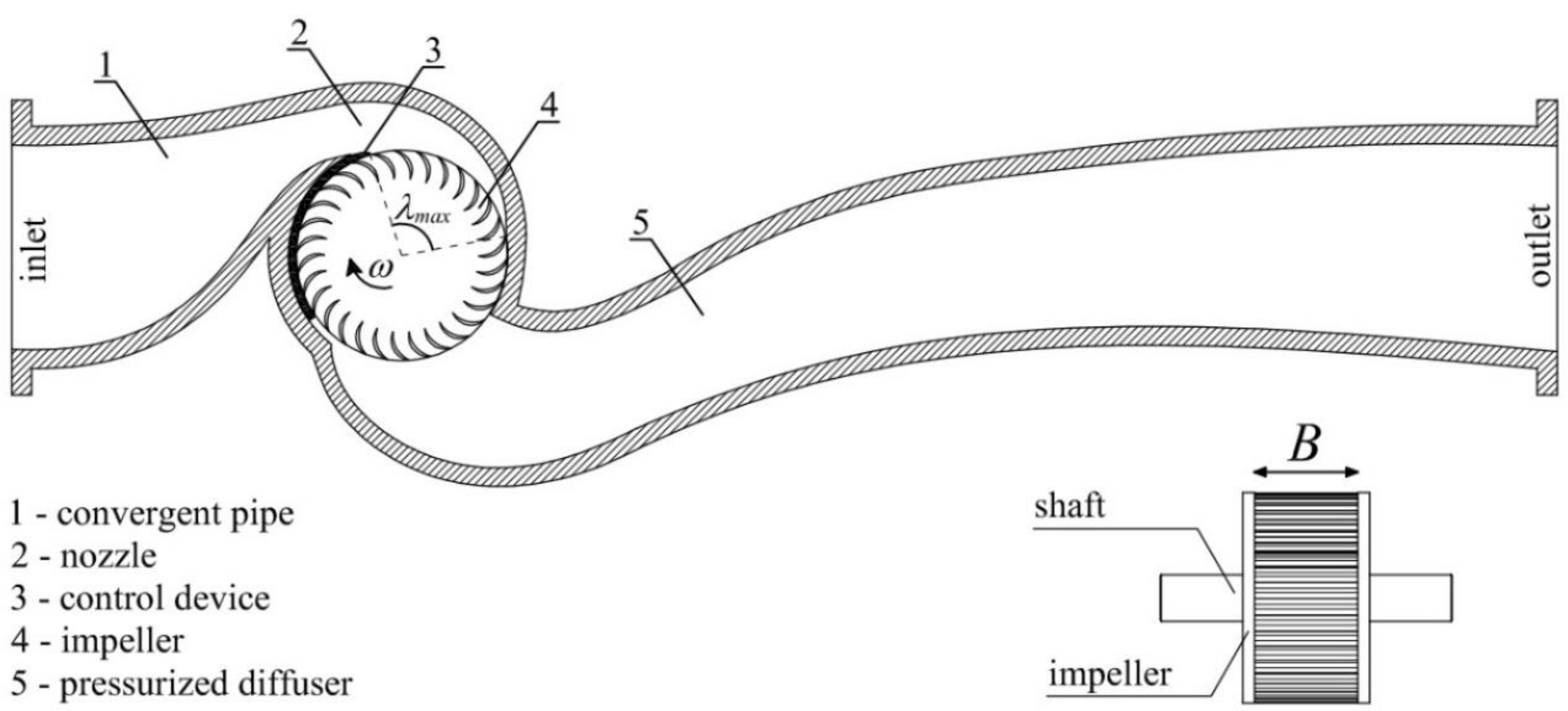
PRS is a new inline turbine with a mobile regulation flap, a pressurized diffuser, and the same impeller of the crossflow turbine (Figure 1).
The design procedure for PRS is divided into three parts: (1) design of rotational velocity, impeller diameter, and width; (2) stator design; (3) design of blade shape and number.
The first and second parts have already been proposed by the present authors [14] and will now be briefly summarized. The water jet velocity inside the turbine is given by Equation (1):
where CV = 0.98 and ξ = 2.1 are constant coefficients [13], ΔH is the head drop between inlet and outlet PRS sections, ω is the impeller rotational velocity, D is the outer impeller diameter, and g is the gravity acceleration. The momentum Equation (1) can be coupled with the relative velocity optimality condition, which is represented by Equation (2):
where Vr is the optimal velocity ratio, for PRS turbines equal to 1.7 [14] and α is the velocity inlet angle, with respect to the tangent direction, approximately equal to 15°. For a given value of the impeller rotational velocity ω, usually chosen among a finite number of possible speeds of the electric generator coupled to the turbine, Equations (1) and (2) can be solved in the V and D unknowns. Note that the rotational velocity ω is function only of the frequency f of the alternating current (AC) grid and of the number p of the polar couples of the electrical generator coupled to the turbine, according to the following equation:
3. Fluid Dynamic Investigation
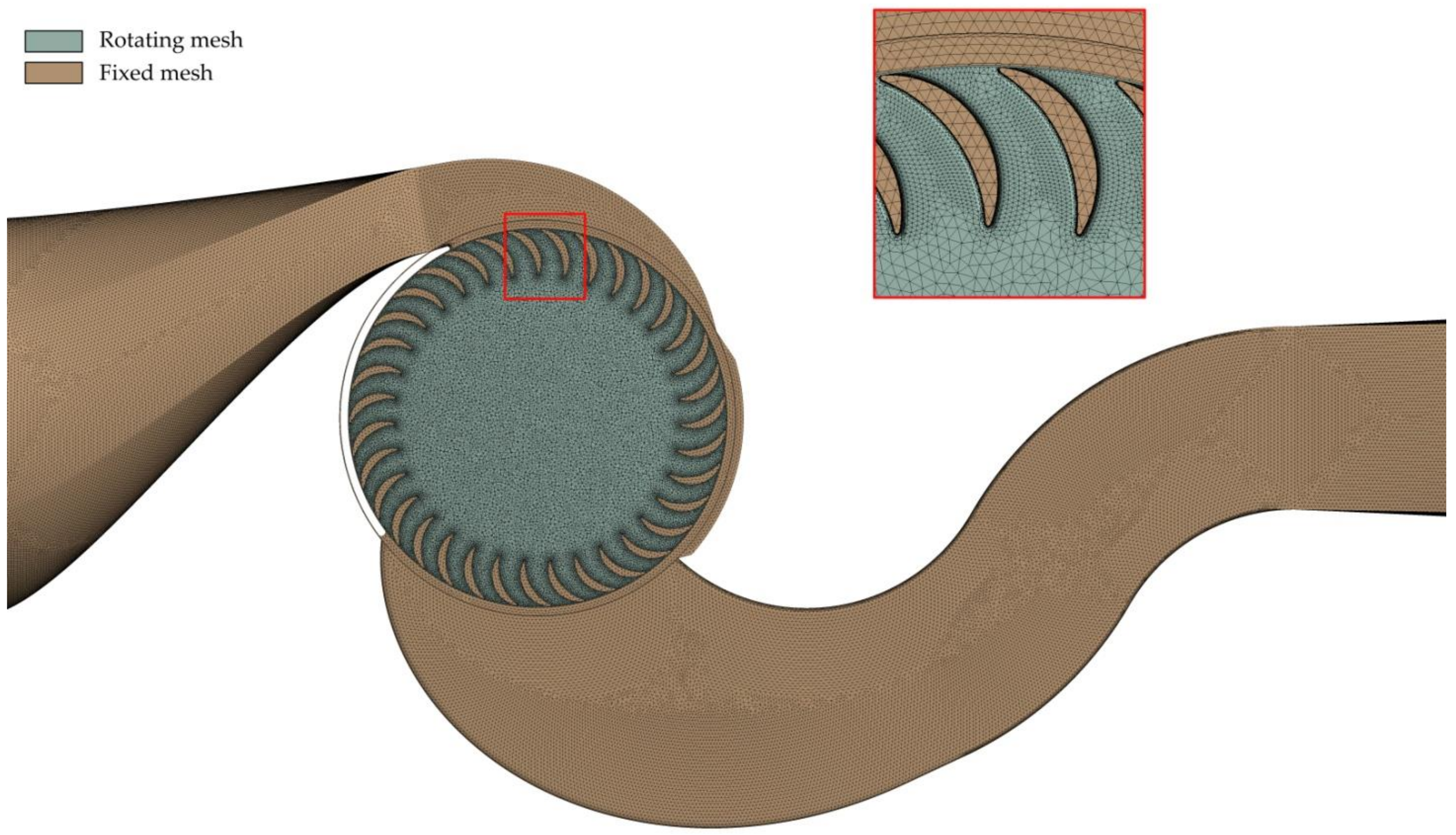
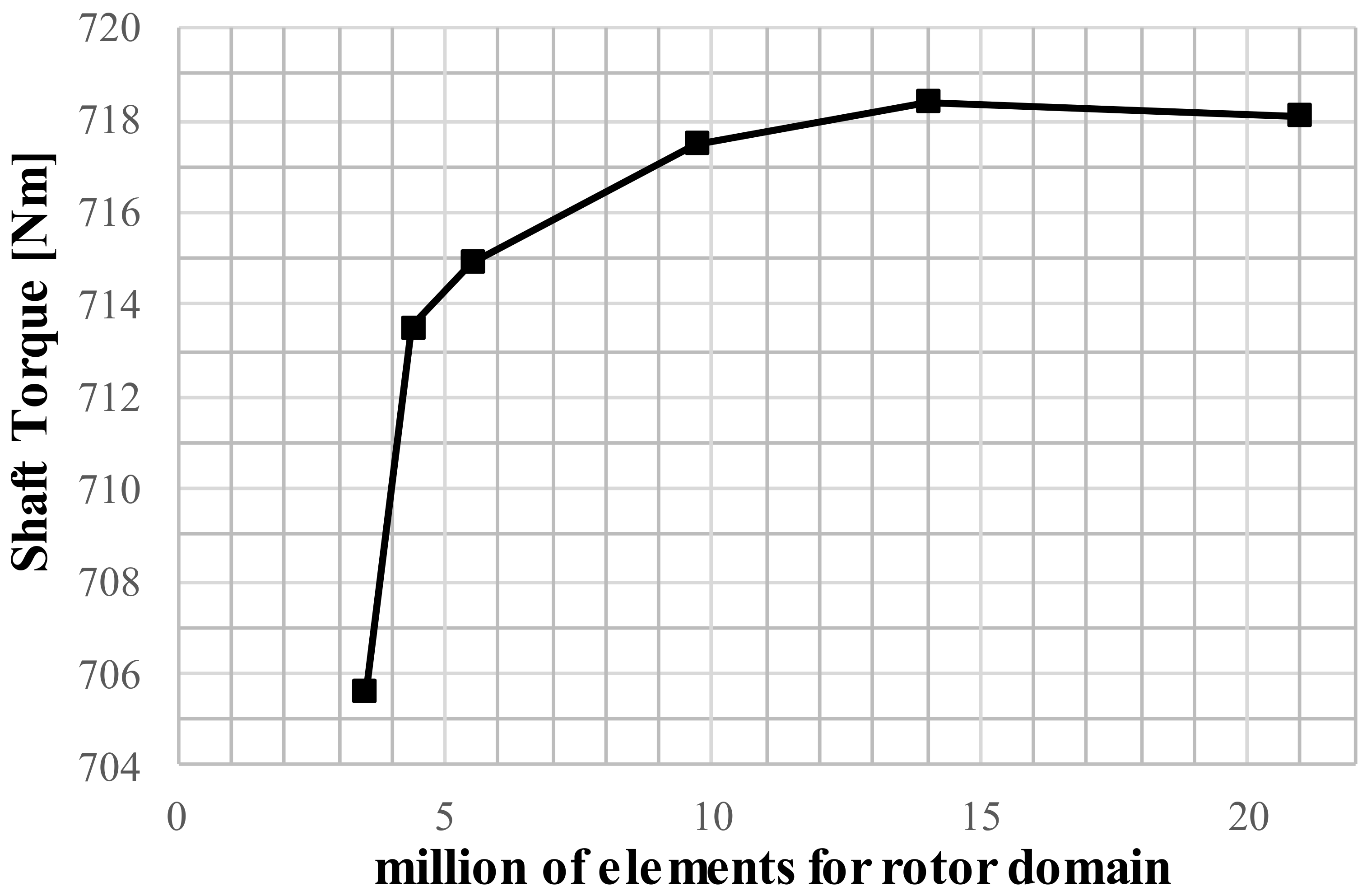
Optimal impeller design could be achieved through a set of 3D CFD simulations, coupled with associated structural 3D FEM analysis. However, this approach is computationally very intensive and, using standard computers, each simulation would take many weeks or even months of numerical calculation. The 2D and 3D CFD models of the PRS turbine have already been studied and validated with experimental and field data from the same authors in previous works [13,14,15,16]. In the present study, the same models have been applied for the design of two different machines, named PRS1 and PRS2 (Table 1). For each of them, the computational domain was divided into two sub-domains: the stator (convergent pipe, nozzle, and pressurized diffuser, see Figure 1), with an inertial reference system; the rotor (impeller), with a non-inertial reference system. Both domains were discretized into tetrahedral and prismatic elements and the mesh density was increased until an almost constant shaft torque was achieved. See Figure 2—the final domain discretization of PRS1 turbine in the 3D model, and in Figure 3—the shaft torque plotted versus the corresponding number of elements of the rotor domain.
Note that with more than 14 million elements in the rotor domain, the shaft torque increment becomes negligible. For this reason, we selected this grid as the optimal one.
Simulations were carried out using the Ansys CFX commercial code, solving the Reynolds-averaged Navier Stokes (RANS) equations [12,18]. CFX gives the option to select one among different advection models. We chose the high-resolution scheme, which uses second order differencing for the advection terms in flow regions with low variable gradients [18]. The high-resolution scheme uses the first order advection terms in areas where the gradients change sharply, to prevent overshoots and undershoots, and maintain robustness. The RNG k-epsilon turbulence model was selected in the CFX code, according to previous studies [12]; the interface between the stationary and rotating domains was the transient rotor-stator type. The time step adopted for each run was 2.5 × 10⁻⁴ s. The root mean square residual was used for the convergence criterion with a residual target equal to 1.0 × 10⁻⁵. The boundary conditions selected in the simulation according to the design data are the following: (a) the total pressure per unit weight at the nozzle inlet, corresponding to the piezometric level plus the kinetic energy per unit weight, (b) the flow rate at the outlet section of the casing. The initial condition for unsteady state simulation was the fluid field output computed, according to the steady state flow assumption.
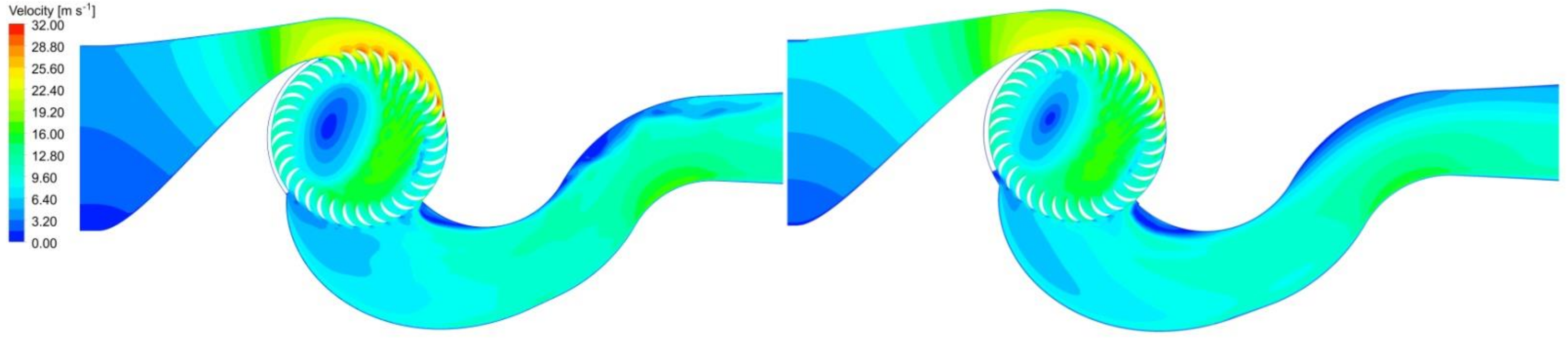
Due to the symmetry of the impeller, with respect to a plane normal to its axis, the difference between the 2D and the 3D solution of a Banki type turbine is usually small [20]. Most important, this difference does not affect the optimality of the 2D parameters, because the reduction of efficiency observed in 3D models is not dependent on their setting. To this end, Table 2 provides the efficiencies computed by solving three different configurations of the PRS1 turbine using 2D and 3D models. The 3D efficiencies are all below the 2D ones, but the optimal configuration is the same for both models. Adopting the 2D assumption, the velocity and the pressure field of the PRS1 turbine described in Table 1 was computed with a CPU time of only 20 h. Figure 4 shows the velocity field in the symmetry plane of the 3D simulation (left) and the 2D simulation (right). The results show a good match for the accuracy required by the proposed iterative design procedure.
4. Design of Blade Shape and Number
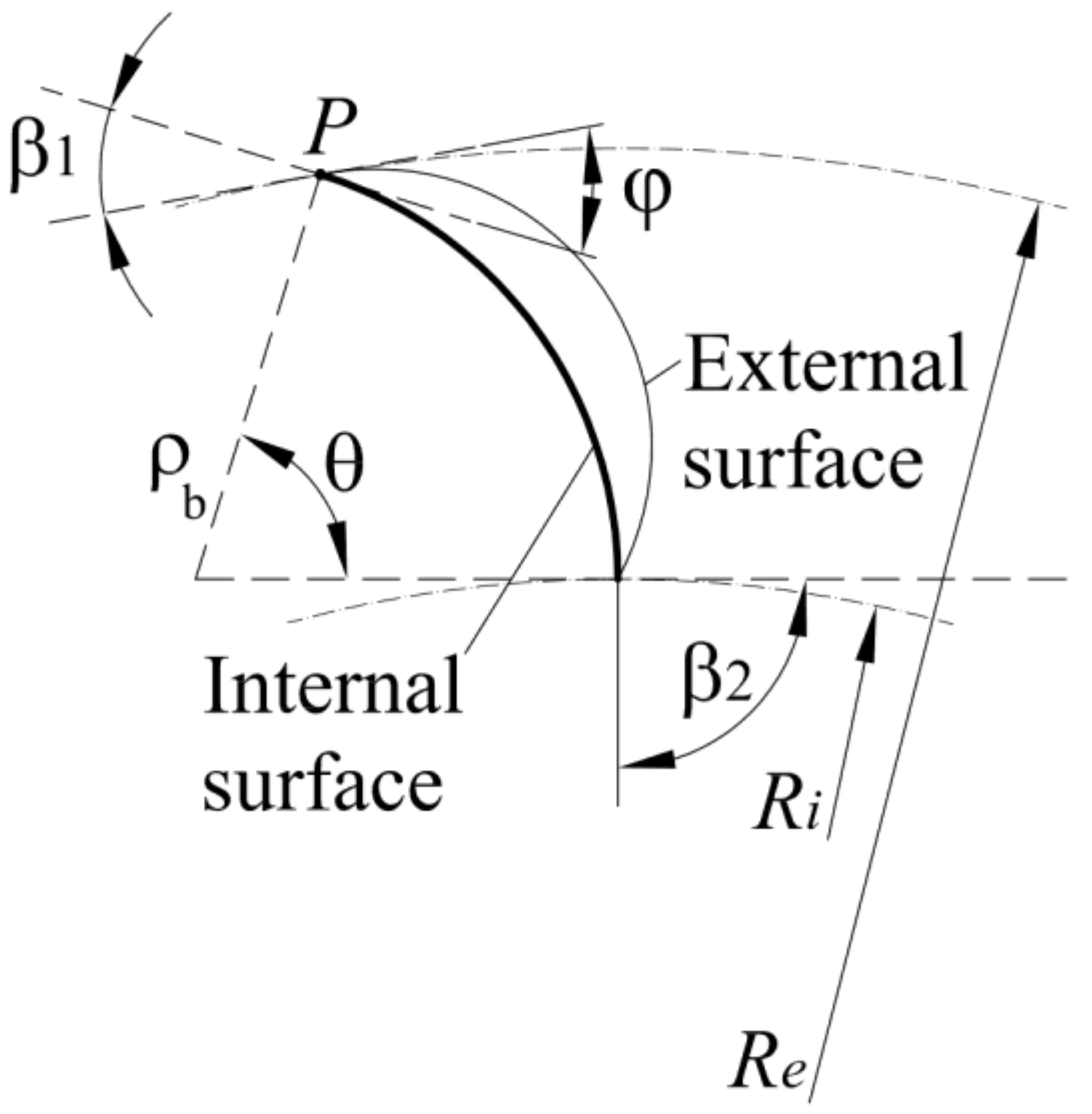
In the proposed new blade section, the internal surface is the same traditional one with circular shape, and the center of the circle is located at the intersection of the two directions orthogonal to the inlet and outlet relative velocities (Figure 5). The exit angle β2 is equal to 90°. The inlet angle β1 guarantees to the inlet water particles a relative velocity tangent to the inlet blade surface. Note that, because the velocity norm V in Equations (1), (2) and (4) represents the mean value along all the inlet impeller surface, the radial velocity component in P is smaller than the mean value, due to the φ angle existing between the directions tangent to the internal and the external surface. This also implies that the velocity ratio in Equation (2) is smaller than the ratio computed using the local velocity in P instead of the mean one. Previous experiments suggest a value equal to 2 [20]. According to this hypothesis, the radius ρb, the angle β1 and the central angle θ of the blade can be computed as a solution of Equation (5), setting the optimal value of the impeller inner diameter ratio Di/D equal to 0.75 [16].
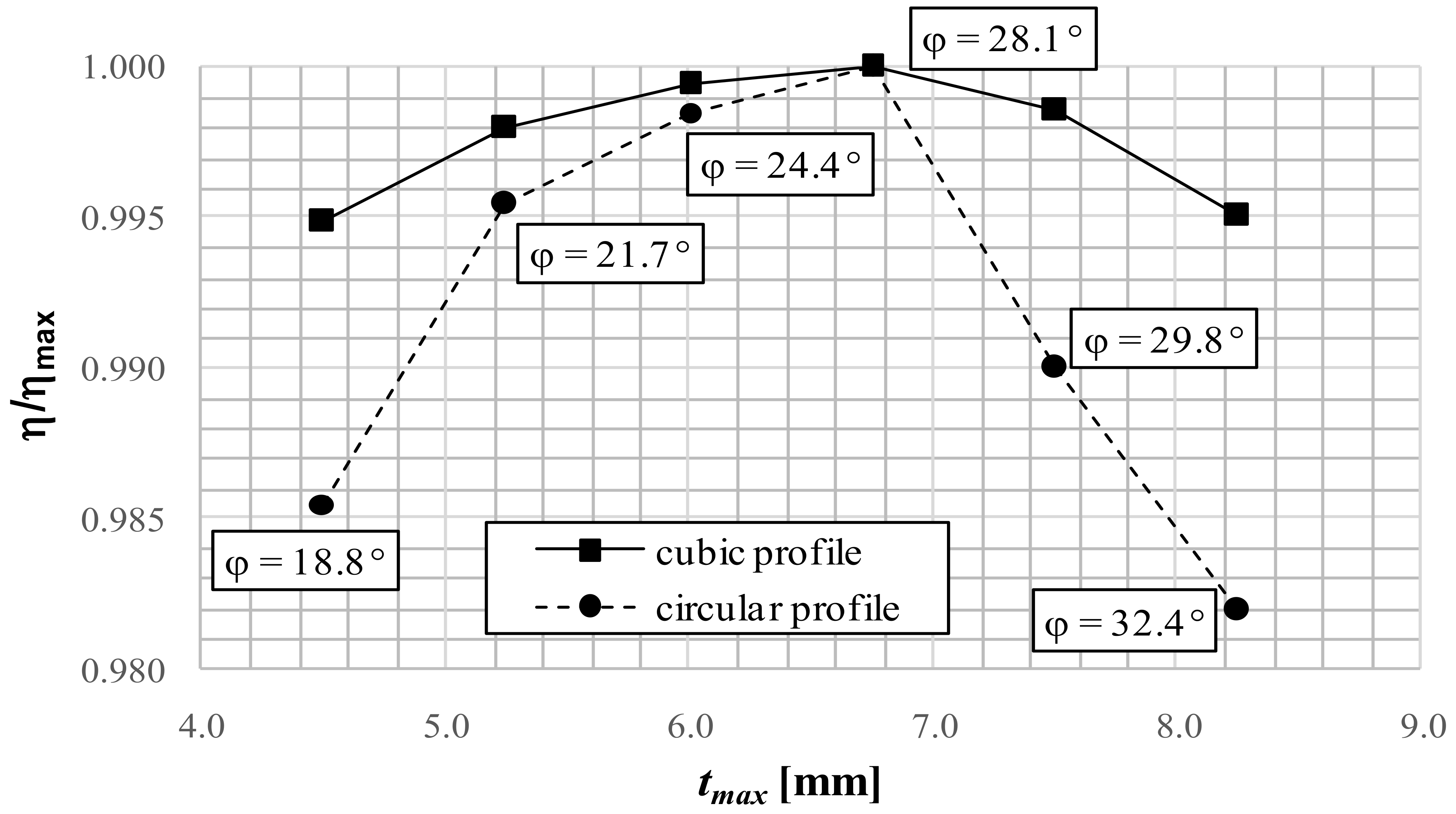
Table 1 lists the parameters of two case studies of the PRS turbine, marked as PRS1and PRS2, with a traditional circular profile of the external surface. Note in Figure 6 the corresponding turbine efficiency computed for several φ values and corresponding maximum thickness tmax, scaled by the best efficiency obtained for an angle φ = β1 (see Figure 5). The efficiencies are computed with 2D CFD simulations, setting a fixed pressure value in the inlet and outlet boundaries. The number of blades is optimized for each couple of φ and tmax values. Sharp edges are well known to provide a local stress concentration along the same edges, which can be avoided by rounding off the edges with a circular profile, as shown in Figure 7a. A value tmin = 0.1 tmax corresponds to a maximum stress located outside the edge, without a significant reduction of the hydraulic efficiency with respect to the value obtained with tmin = 0. We note in Figure 6 that the maximum efficiency is computed for both PRS1 and PRS2 with φ = β1, corresponding to an external surface tangent to the inlet impeller surface. The reason is likely to be that the increment of the φ angle provides a reduction of the α attack angle of the water particles along a large part of the channel inlet, and a corresponding efficiency increment. For φ values larger than β1, the attack angle becomes negative, with a sharp efficiency reduction.
Let us call tmax,opt the maximum thickness corresponding to the condition φ = β1. Note that, if the maximum thickness does not guarantee the blade structural resistance and the computed maximum von Mises stress is higher than the admissible limit, we need to give up the maximum efficiency condition in favor of a more robust design.
The previous results show how the maximization of the efficiency of simply circular blades can lead to a poor mechanical design. To avoid that, we change the profile of the external surface moving from a second-order (circular) to the following third-order (cubic spline) profile:
where t is the thickness along the radial direction, orthogonal to the internal surface, and δ is the angle between the radial directions at (1) the given point and (2) the intersection of the internal blade surface with the impeller inlet (Figure 7a). Coefficients a, b, c, and d are computed by setting:
where tmax is the maximum thickness, tmin is the minimum thickness at the outlet extremity, t’ is the derivative with respect to δ in the interval (δmin; θ), tmin is empirically set equal to 0.1 tmax and δ* is a fifth auxiliary unknown.
t’(δmin) = tan(β1 − δmin)
t(δmin) = t0
t(θ) = tmin
t(δ*) = tmax
t’(δ*) = 0
The angle δmin and the thickness t0 are the parameters of the tip of the blade and are computed to guarantee the tangent condition of the external blade surface to the impeller inlet surface. The inner blade extremity has a circular profile with radius rf, tangent in point P1 to the cubic spline profile of the external surface and in P2 to the circular profile of the internal surface (Figure 7b). rf is empirically set equal to 0.1 tmax.
Equations (7–11) guarantee the tangent condition of the external surface to the inlet impeller surface for different possible values of the maximum thickness. Figure 8 shows how the cubic profile allows to maintain high efficiencies, in the PRS1 turbine, while changing the tmax thickness value.
5. Maximum von Mises Stress Computation
The total power at the turbine shaft is obtained by summing the torque of each blade multiplied by the rotational velocity of the impeller.
Let us define as τ the ratio between the power provided by a single blade and the total available hydraulic power, which is:
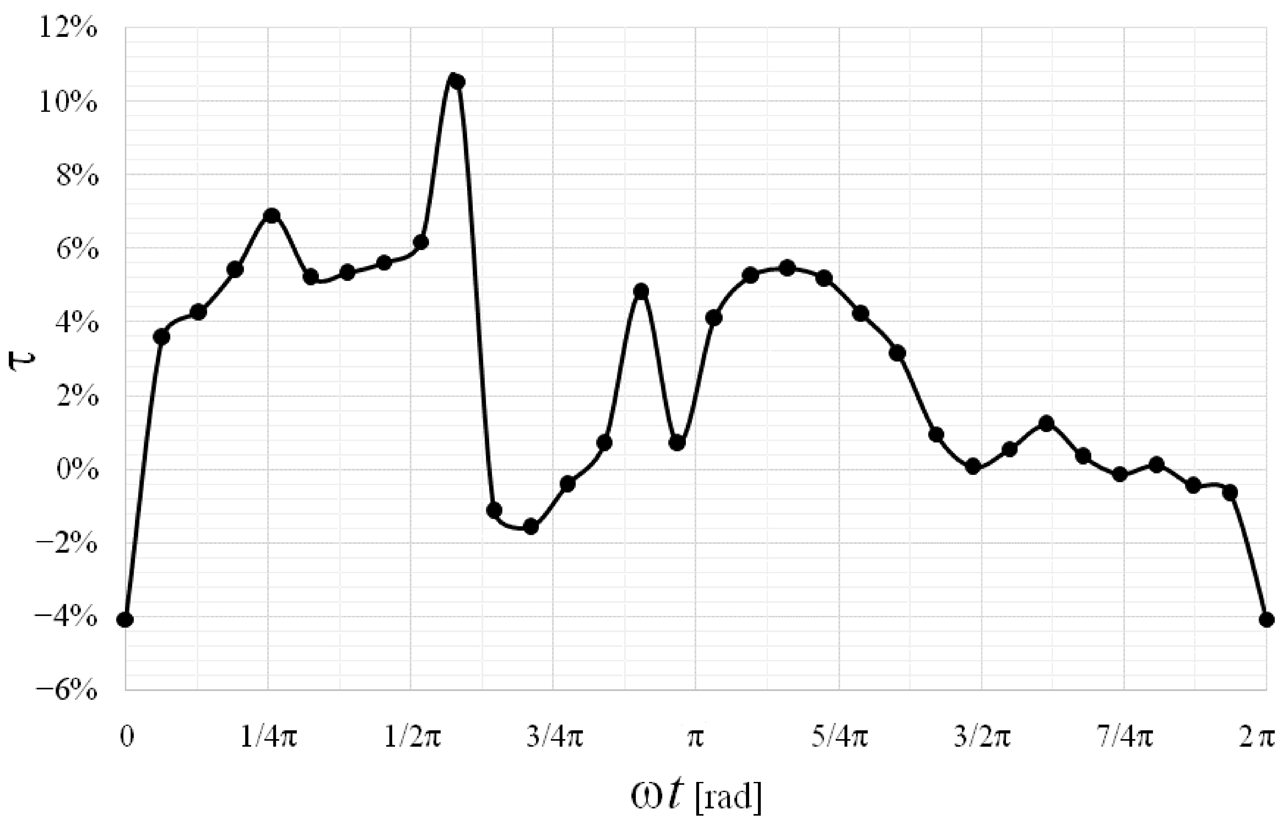
In crossflow impellers, the torque of the blades at a given time is not the same, because it depends on the position of the blade itself. Figure 9 shows the τ distribution obtained in PRS1 turbine for a given blade, as function of its position. The total number of blades was 31.
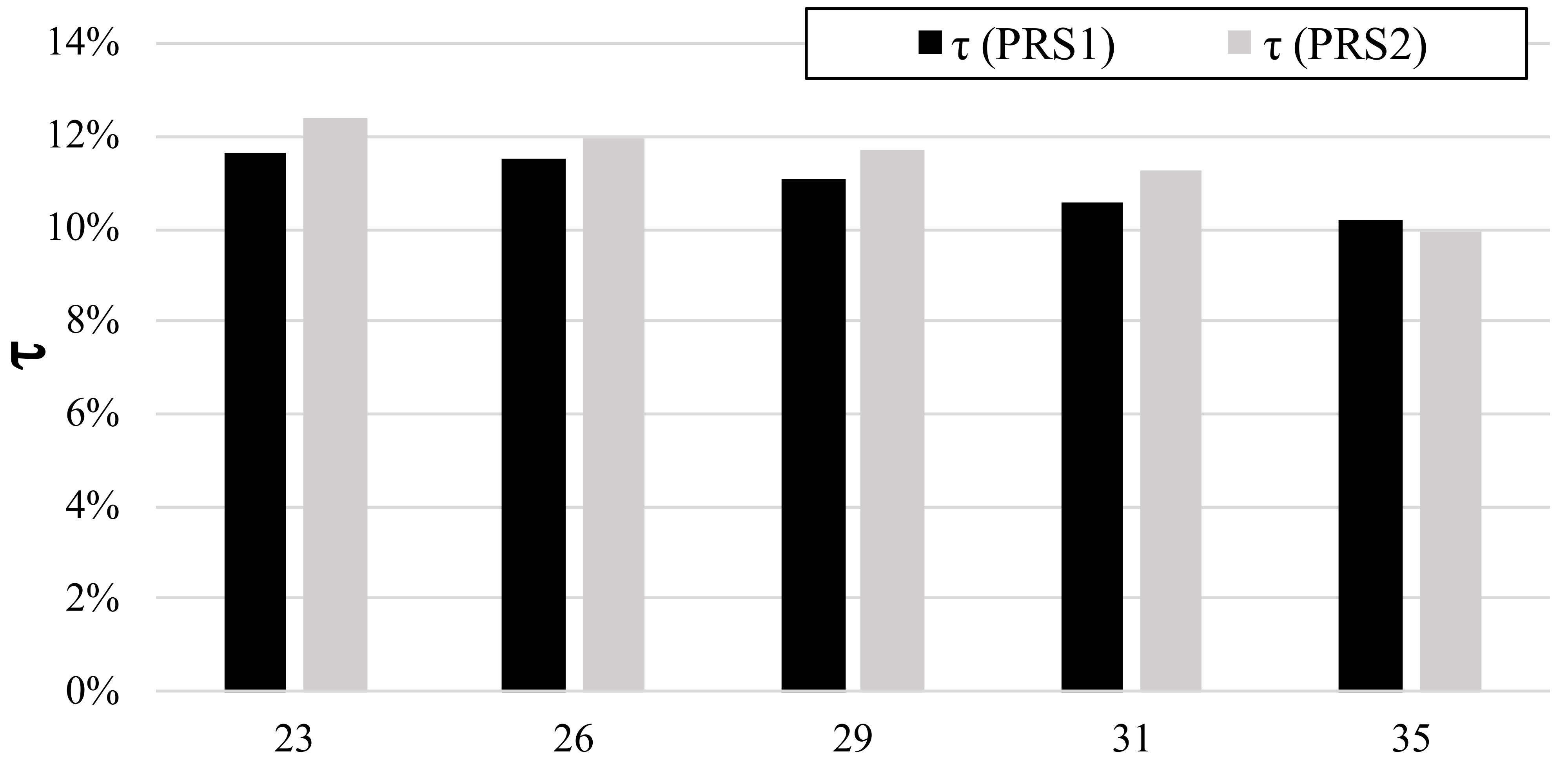
The trend of τ shows a strong variation since, as is well known, in crossflow turbines the shaft torque is provided by the flow that runs through the impeller in two different stages, known as first and second stages. In the transition between the first and second stages, the blade is stressed in the opposite direction due to the dragging action it exerts on the fluid, which does not constitute the main jet. The contribution to the overall power of the first stage is always greater than the second stage, with a peak for the single blade, which we call τmax. Using several CFD 2D test cases the behavior of this parameter was analyzed as a function of the number of blades of the impeller, within the range 22–35 suggested by most of the authors (see Table 3). The results obtained for two different impellers are summarized in Figure 10. We can observe that the maximum value of the ratio τ drops very slowly, along with the increase in the number of blades, in the analyzed range. For this reason, the maximum von Mises stress s is initially assumed independent from the number of blades.
For the same turbine, two operating configurations return two different values of the maximum stress. The first one occurs when the impeller is rotating and, therefore, the maximum von Mises stress must be compared with the fatigue limit, due to the high frequency of the load cycle in each blade. The second configuration occurs when the impeller is still, but is crossed by a discharge corresponding to the maximum head drop (greater than the maximum discharge at work) and the Mises stress can be compared with the yield strength. For the materials usually adopted, the first configuration is more severe than the second one and, for this reason, we carry on the design according to the first configuration and carry on a simple validation for the second one.
Design of the Maximum Admissible von Mises Stress Sadm
Mechanical elements, such as turbine blades, are often subject to loads that vary over time. The load on a mechanical element increases up to the maximum value and then decreases up to the minimum value in a cyclical manner. When a mechanical component is damaged under the action of cyclical tensions, although the values of the nominal stress peaks remain below the tensile stress, collapse occurs due to phenomena caused by fatigue. Some authors argue that 80–90% [27] of failure of structural components is due to these phenomena. To explain the physical mechanism of fatigue damage [28,29], it must first of all be noted that construction materials are never homogeneous and isotropic. Even if no carvings are present, stresses are distributed unevenly, and it is easy to locally exceed the yield limit, even if the nominal stress always remains much lower. Fatigue failure is due to localized damage accumulation, caused by cyclic deformation in the plastic field. Typically, the break occurs after several thousand cycles.
There is not, to date, a mathematical model able to fully describe the fatigue behavior of materials; the empirical approach is the most widely used from a practical point of view.
To determine the strength of a material under the action of fatigue loads the specimens of a particular material are subjected to forces that vary cyclically over time between a maximum and a minimum pre-set value, up to mechanical failure. The curve interpolating the experimental results is known as the Wöhler curve [30], which is plotted in a diagram with number of cycles at failure (Nf) versus nominal stress Sf.
In the Wöhler diagram, we distinguish three Nf ranges:
- A first quasi-static resistance or low cycle fatigue range (Nf < 103÷4), where Sf remains constant;
- A range with a high number of cycles (103÷4 < Nf < 106), where the Wöhler curve equation is of the type Sf µ Nf = K, with µ and K constants relative to the material;
- A third range with a very high number of cycles (Nf > 106) where Sf again remains constant, but much smaller than in the first Nf range.
The nominal stress occurring in the third Nf range is called the fatigue limit, Sl, and is the maximum alternating stress value at which no breakage occurs. Experimental tests show that, for steel, the fatigue limit varies between 40 and 60% of the tensile strength Sr, and the average fatigue limit for rotating bending specimens can be obtained with the following relationships:
- Sl = 0.5 Sr for Sr < 1400 MPa;
- Sl = 700 MPa for Sr > 1400 MPa.
6. The Proposed Methodology for Impeller Design
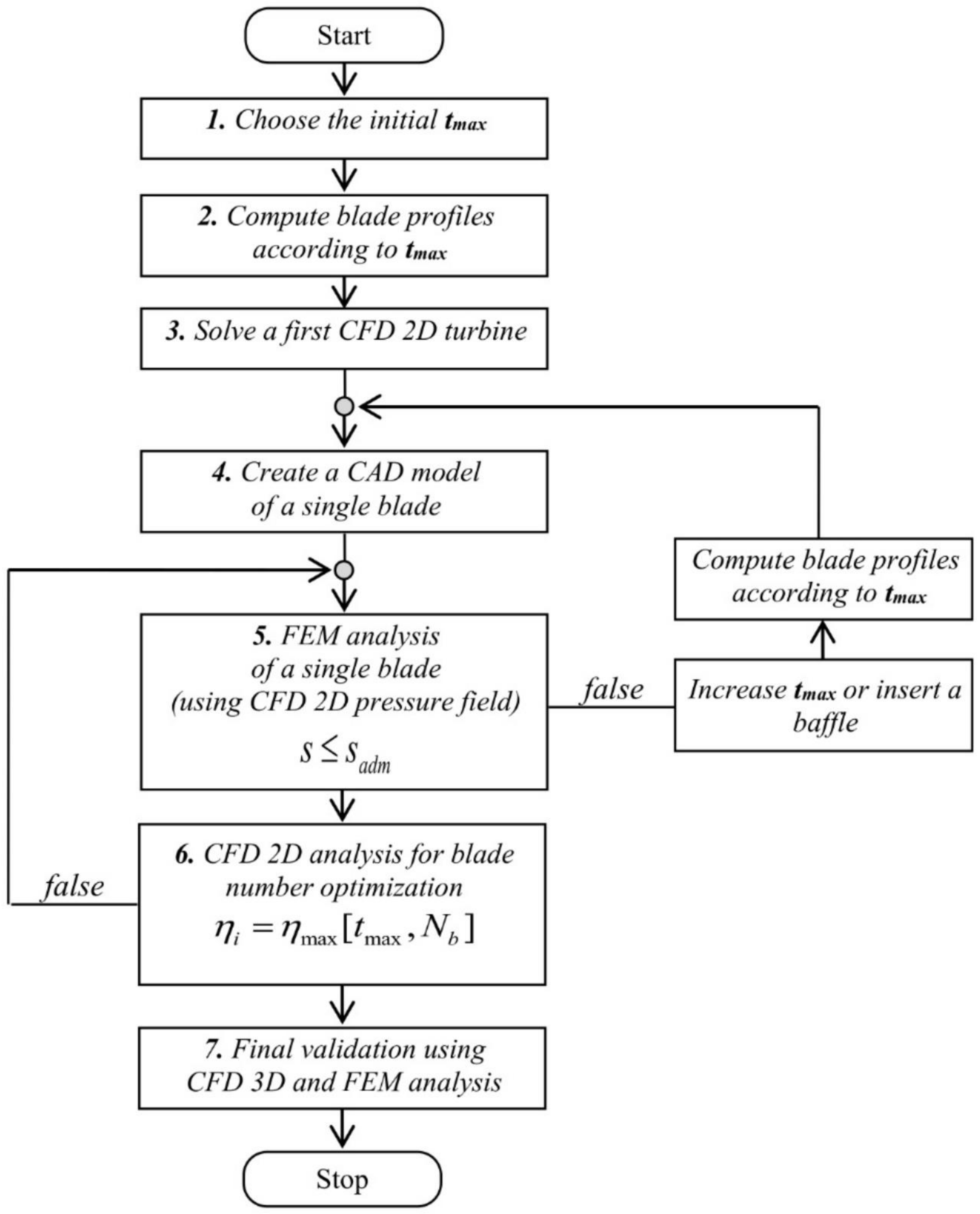
The proposed methodology can be summarized in the following steps:
- Compute width B and diameter D according to the procedure described in Section 2. Choose a small maximum blade thickness tmax, as the initial tentative value.
- Compute the internal and external blade profiles according to the procedure explained in the previous section.
- Solve a first 2D CFD model using an impeller with 35 blades, which is the upper limit of the usual range, and export the pressure distribution on the blade surface.
- Create a 3D CAD model of a single blade, based on the impeller width B and on the previously computed profile. Add to the CAD model a small portion of the two disks at the lateral contours of the blade; compute the fillet radius at the blade-disk connection and, after the first iteration, at the connection with eventual baffles. After the first iteration, use the pressure field on the blade previously computed in point 6.
- Using a 3D FEM code, compute the stress field and the maximum von Mises stress S in the selected blade.
- If the maximum thickness used in point 4 leads to a maximum von Mises stress value above the admissible one, here indicated as Sadm, then a new attempt must be made. To this end, either increase the maximum thickness or introduce a new reinforcing baffle. Using the new geometry, compute again the corresponding blade section and update the number of blades with the optimal one corresponding to the new maximum thickness by iteratively solving a 2D CFD model. Update the pressure distribution on the blade surface and go back to point 5. The trial and error procedure must be repeated until the computed maximum stress is below the admissible one.
- Perform a final validation of the impeller geometry using only one 3D CFD simulation coupled with 3D FEM analysis.
The above procedure is shown in the flow chart of Figure 11. In the following, the single steps will be explained in detail.
To compute the profiles of the internal and external surface, an initial value for the maximum thickness tmax is required. A reasonable choice would be to start with a small reliable value and gradually increase it until the maximum von Mises stress is less than Sadm.
Once the cross-section of the blade is designed in step 2, a 3D CAD model of a blade with a length equal to the width B of the impeller has to be designed in step 4. See, in Figure 12, the blade obtained in the next case study, adopting t = 7 mm and B = 55 mm.
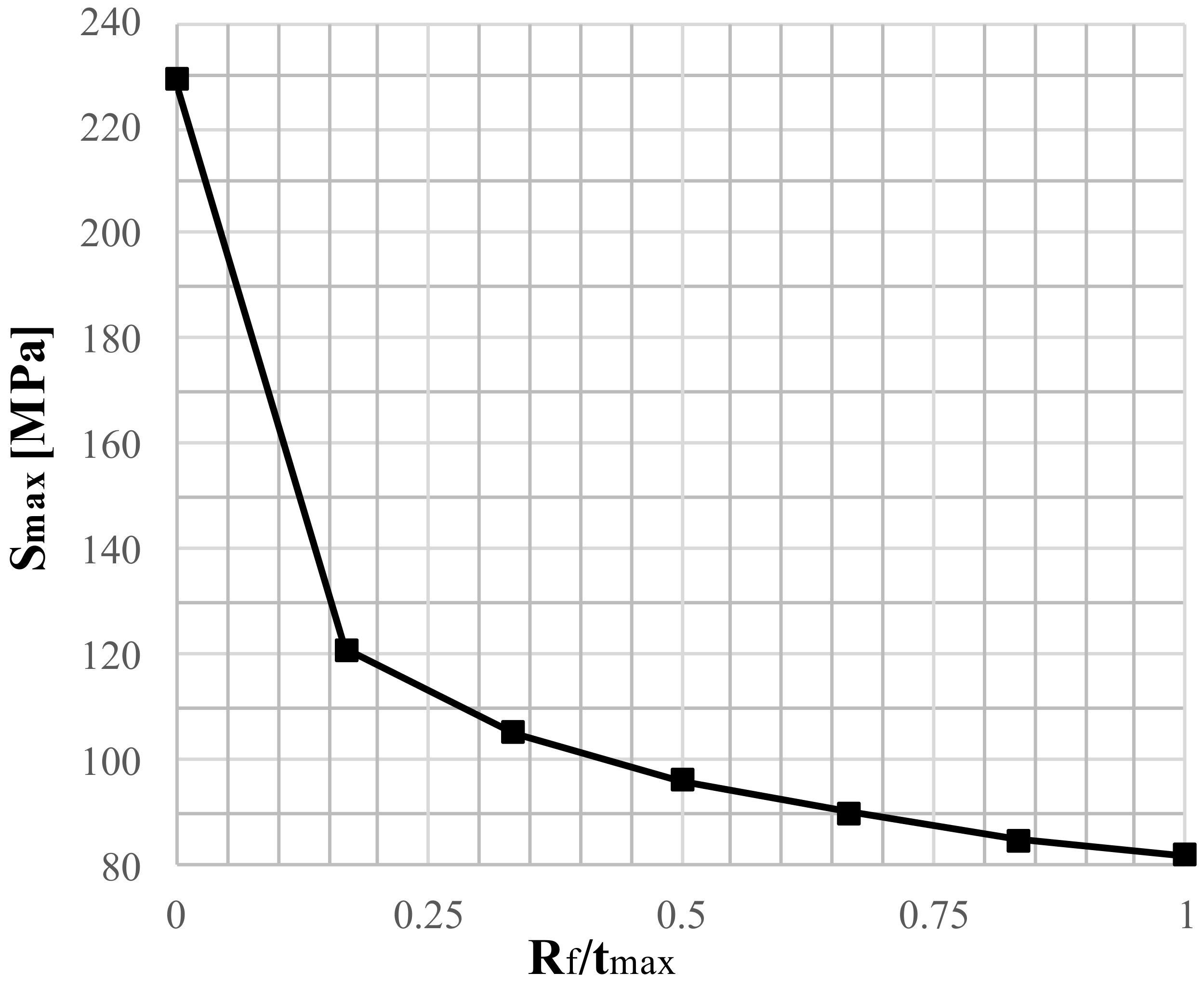
To complete the CAD model required in this approach for the FEM analysis, a small portion of the two disks at the ends of the blade needs to be added. If the impeller design includes one or more intermediate baffles, it is also necessary to design a part of it. A connection radius, Rf, must be introduced at the blade-baffle connection. A fillet radius is always present in the real impeller and cannot be neglected to avoid exceptionally high stresses along the surface intersections. A parametric study was carried out to determine an approximate optimal value of the fillet radius as a function of the maximum thickness t for different impellers.
As expected, the peak stress level first decreases very quickly when the fillet radius increases; then the reduction becomes slower and slower (see Figure 13). It was found that the stress level seems to converge for values of Rf/tmax ratio higher than 0.833. A ratio Rf/tmax = 0.833 is also a reasonable design choice.
In Figure 14 a CAD model of one blade, including a small portion of the two disks at the ends of the blade, and a part of a reinforcing baffle, are shown.
In order to validate the blade stresses, a FEM analysis is carried out by loading the blade with the pressures obtained by the CFD 2D iterative analyses, assuming a constant pressure along the width.
In the structural analysis, one of the two modeled portions of disk must be fixed and a constraint must be imposed on the baffle to allow only a rotation around the axis of the turbine and to block all the other DOFs (Degrees of Freedom). The structural simulation will make it possible to compute the von Mises stresses of the blade. In particular, the maximum stress value in a crossflow hydraulic turbine should be much lower than the fatigue limit of the material. If this condition is verified the CFD 2D simulations will make it possible to obtain the maximum efficiency by optimizing the number of blades for a known maximum thickness t. Otherwise, the procedure must be repeated by increasing the thickness t or by inserting a baffle.
Final validation of the entire impeller is carried out by performing a single 3D CFD simulation including a structural FEM analysis.
7. A Case Study: Fontes Episcopi Power Plant
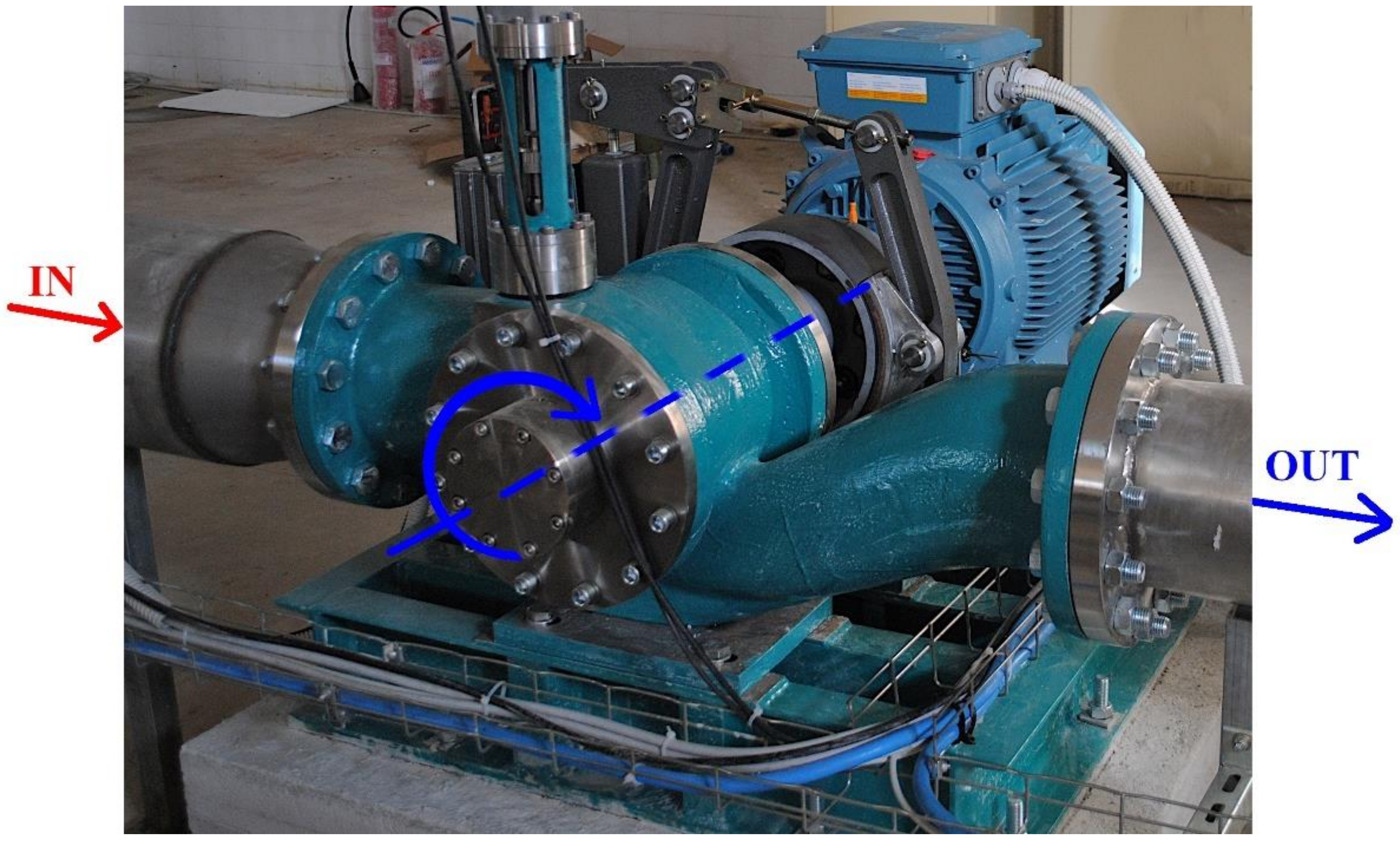
We applied the proposed procedure for the design of a PRS turbine already installed in a pressure regulation hydraulic node, named Fontes Episcopi, which is part of a larger Water Transport Network of Sicily (Italy), named Gela–Aragona. The installed PRS turbine (Figure 15) was designed with the following input parameters: ΔH = 100 m, Q = 100 l/s and ω = 1500 rpm, and the results of the field tests were reported in a previous work by some of the authors [13]. Unfortunately, the operating conditions (ΔH and Q) actually occurring in the site were different from the design input parameters and the turbine, in the start-up period, worked with a mean efficiency of only 61%. Using the same input parameters and an inlet angle λmax = 110° (Figure 1), a new PRS turbine, called PRS2, was designed with the proposed procedure, according to the input parameters listed in Table 1. Trough Equations (1–4), the resulting impeller diameter D and width B were found to, respectively, be 234 and 55 mm.
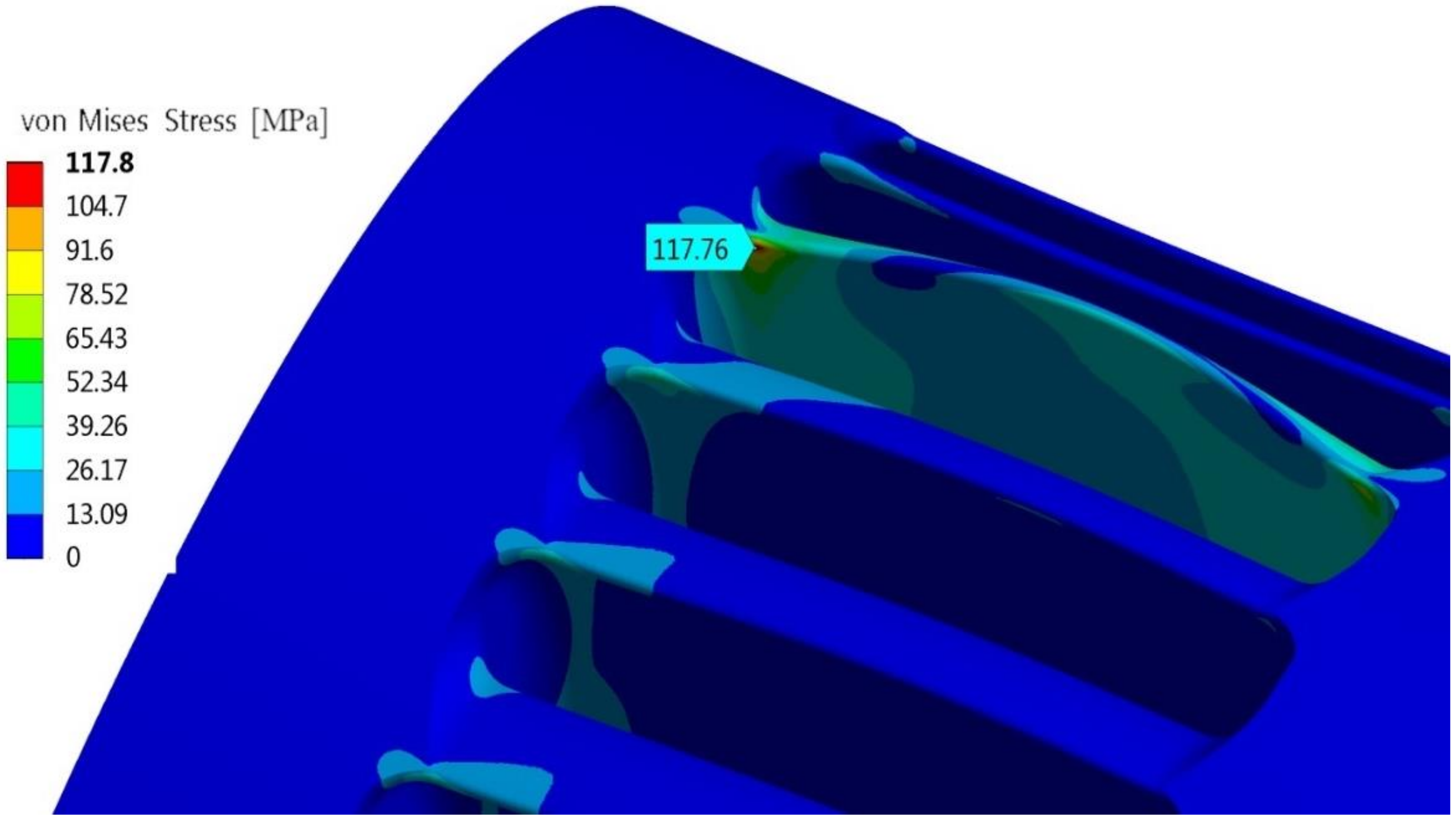
Three different impellers, made of stainless steel, were designed using traditional blade design (impeller 1 and 2) and the new proposed blade design (proposed impeller). The tensile strength for stainless steel, Sr, was set equal to 500 MPa, with a corresponding fatigue limit Sl equal to 250 MPa. Application of a reasonable safety factor 3 [31,32] provided Sadm = 250/3 MPa = 83.3 MPa. The external surface of the blades of impeller 1 had a circular profile. The corresponding maximum efficiency was η = 79.3%, attained for φ = β1, tmax = 5.12 mm and a number of blades equal to 34. The maximum von Mises stress Smax = 117.76 MPa was not lower than the admissible limit Sadm (see Figure 16, where the stress is the result of 3D FEM analysis).
If the condition φ = β1 is relaxed, it is possible in impeller 2 to increase tmax up to 7 mm, corresponding to an optimal number of blades equal to 27 (computed by CFD 2D analyses, and not reported here for brevity). In this case, the maximum von Mises stress is less than Sadm (see Figure 17) but the efficiency decreases up to η = 78.2%.
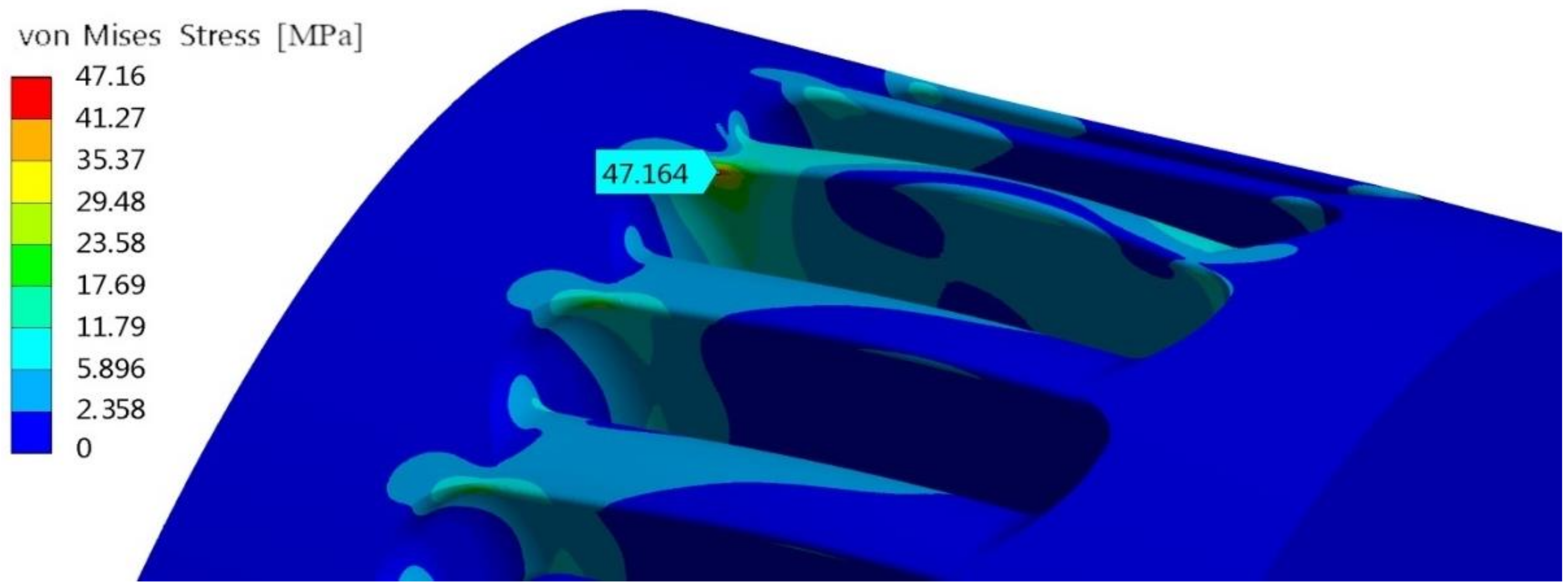
The external surface of the blades of the proposed impeller had a cubic profile, as computed according to the procedure described in Section 5, with φ = β1, tmax = 7 mm and nb = 27. The resulting efficiency value was η = 79.2% and the maximum von Mises stress was below the admissible limit Sadm (see Figure 18).
The von Mises stress obtained by FEM analysis of a single blade (Figure 19) was similar to the final one computed with a CFD simulation coupled with a FEM analysis of all the impeller (Figure 18) and equal to 45.91 MPa.
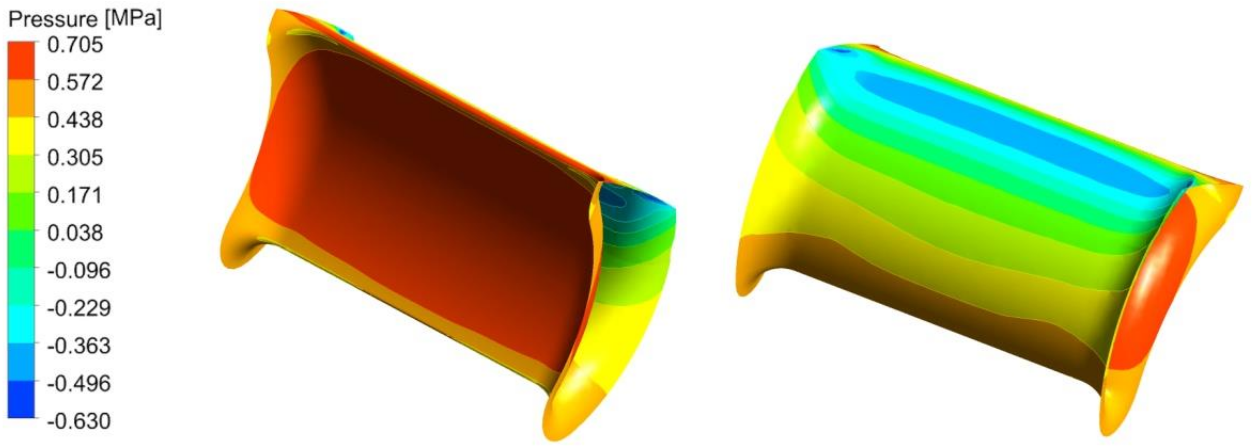
In Figure 20, the pressures on the internal and external surface of the most loaded blade, computed by the final 3D CFD analysis, are shown. The hypothesis of a constant pressure holding along the width for the most stressed blade is approximately validated.
The PRS with the proposed impeller had the best efficiency and the corresponding maximum von Mises stress was always below the admissible limit. Results are summarized in Table 4.
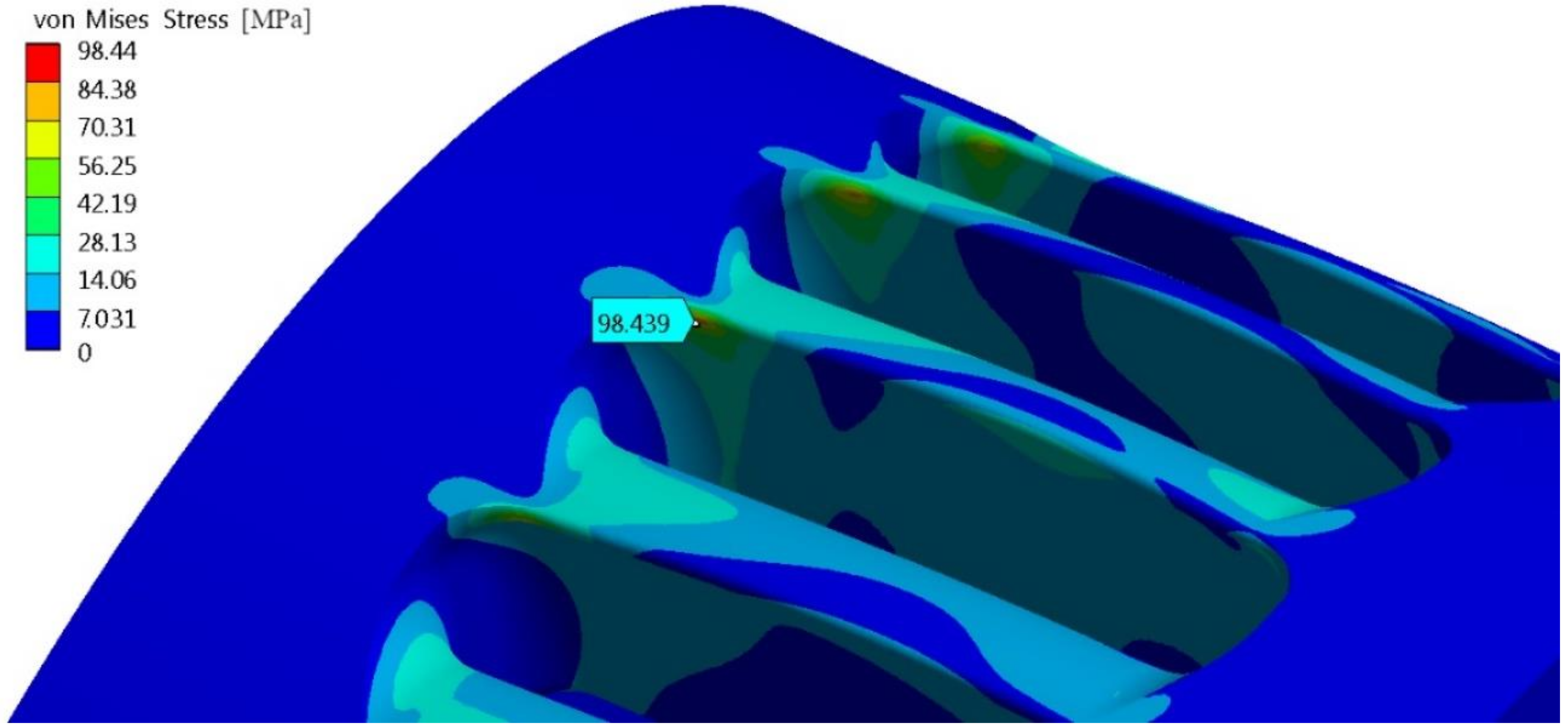
In the real installation, the PRS is equipped with a negative brake, to be used in the case of sudden failure of the electric network. When the network fails, the brake blocks the impeller rotation, and the water flow increases up to 1.4 times the design value [13]. In this case, the impeller is subject to higher normal stresses than those previously seen, but no cycle occurs. In this case, for the proposed blade profile, the 3D FEM analysis computed a maximum von Mises stress equal to 98.44 MPa (Figure 21), which is lower than the tensile strength, around 215 MPa.
8. Conclusions
A new procedure for the design of the blade profile in crossflow type turbines, coupling hydraulic efficiency with mechanical reliability, is proposed and numerically tested for a real case study. A proper use of 2D-CFD models and 3D-FEM structural models makes it possible to limit the computational effort, in order to achieve the final design within a reasonable time using a standard workstation with a few dozen processors.
In the case study, a total of 30 2D CFD simulations and seven 3D blade structural analyses were carried out, with a total computational time of 600 h on a computer working with several CPU Intel® Xeon(R) E5-2650 v3 processors. The same problem, solved as the search of a 3D coupled structural and hydrodynamic optimization of the whole impeller, subject to the admissible stress constraint, would require a computational time of 16 days per simulation. Even with only two optimization parameters (number of blades and maximum thickness), the required computational time would have been larger than the actual one of several orders of magnitude.
The new methodology is also based on the non-circular profile of the external surface of the blades. Because crossflow turbines are often selected due to their constructive simplicity, this particular shape seems to be in conflict with the previous motivation. On the other hand, the size of the crossflow impellers remains very small, also for very high power levels. Growing 3D printing technologies allow inexpensive construction of molds with very complex geometries but limited size, where mechanical components, such as the whole impeller, can easily be obtained by fusion. The cost of the impeller, made with this new technology, turns out to be much smaller than the cost required using standard technologies for blades with a circular profile.
Author Contributions
Conceptualization, M.S. and T.T.; methodology, M.S., T.T., C.A., and A.P.; validation, A.P., C.P., Z.D., and M.S.; investigation, M.S., T.T., C.A., A.P., and C.P.; data curation, C.P., A.P., and C.A.; writing—original draft preparation, M.S., T.T., C.A., A.P., and C.P.; writing—review and editing, M.S., T.T., C.A., A.P., and C.P.; visualization, C.P. and M.H.; supervision, T.T. and Z.D. All authors have read and agreed to the published version of the manuscript.
Funding
This research received no external funding.
Institutional Review Board Statement
Not applicable.
Informed Consent Statement
Not applicable.
Conflicts of Interest
The authors declare no conflict of interest.
References
- Fecarotta, O.; Aricò, C.; Carravetta, A.; Martino, R.; Ramos, H.M. Hydropower Potential in Water Distribution Networks: Pressure Control by PATs. Water Resour. Manag. 2015, 29, 699–714. [Google Scholar] [CrossRef]
- Carravetta, A.; Fecarotta, O.; Sinagra, M.; Tucciarelli, T. Cost-Benefit Analysis for Hydropower Production in Water Distribution Networks by a Pump as Turbine. J. Water Resour. Plan. Manag. 2014. [Google Scholar] [CrossRef]
- De Marchis, M.; Milici, B.; Volpe, R.; Messineo, A. Energy Saving in Water Distribution Network through Pump as Turbine Generators: Economic and Environmental Analysis. Energies 2016, 9, 877. [Google Scholar] [CrossRef] [Green Version]
- Carravetta, A.; Del Giudice, G.; Fecarotta, O.; Ramos, H.M. PAT Design Strategy for Energy Recovery in Water Distribution Networks by Electrical Regulation. Energies 2013, 6, 411. [Google Scholar] [CrossRef] [Green Version]
- Nakamura, Y.; Komatsu, H.; Shiratori, S.; Shima, R.; Saito, S.; Miyagawa, K. Development of high-efficiency and low-cost shroudless turbine for small hydropower generation plant. In Proceedings of the ICOPE 2015—International Conference on Power Engineering, Yokohama, Japan, 30 November–4 December 2015. [Google Scholar]
- Samora, I.; Hasmatuchi, V.; Münch-Alligné, C.; Franca, M.J.; Schleiss, A.J.; Ramos, H.M. Experimental characterization of a five blade tubular propeller turbine for pipe inline installation. Renew. Energy 2016, 95, 356–366. [Google Scholar]
- Vagnoni, E.; Andolfatto, L.; Richard, S.; Münch-Alligné, C.; Avellan, F. Hydraulic performance evaluation of a micro-turbine with counter rotating runners by experimental investigation and numerical simulation. Renew. Energy 2018, 126, 943–953. [Google Scholar] [CrossRef] [Green Version]
- Sammartano, V.; Aricò, C.; Sinagra, M.; Tucciarelli, T. Cross-Flow Turbine Design for Energy Production and Discharge Regulation. J. Hydraul. Eng. 2014. [Google Scholar] [CrossRef]
- Sinagra, M.; Sammartano, V.; Aricò, C.; Collura, A. Experimental and Numerical Analysis of a Cross-Flow Turbine. J. Hydraul. Eng. 2015. [Google Scholar] [CrossRef]
- Sammartano, V.; Filianoti, P.; Sinagra, M.; Tucciarelli, T.; Scelba, G.; Morreale, G. Coupled hydraulic and electronic regulation of cross-flow turbines in hydraulic plants. J. Hydraul. Eng. 2017, 143, 04016071. [Google Scholar] [CrossRef]
- Adhikari, R.; Wood, D. The design of high efficiency crossflow hydro turbines: A review and extension. Energies 2018, 11, 26. [Google Scholar] [CrossRef] [Green Version]
- Sammartano, V.; Morreale, G.; Sinagra, M.; Tucciarelli, T. Numerical and experimental investigation of a cross-flow water turbine. J. Hydraul. Res. 2016, 54, 321–331. [Google Scholar] [CrossRef] [Green Version]
- Sinagra, M.; Sammartano, V.; Morreale, G.; Tucciarelli, T. A new device for pressure control and energy recovery in water distribution networks. Water 2017, 9, 309. [Google Scholar] [CrossRef] [Green Version]
- Sinagra, M.; Aricò, C.; Tucciarelli, T.; Morreale, G. Experimental and numerical analysis of a backpressure Banki inline turbine for pressure regulation and energy production. Renew. Energy 2020, 149, 980–986. [Google Scholar] [CrossRef]
- Sinagra, M.; Aricò, C.; Tucciarelli, T.; Amato, P.; Fiorino, M. Coupled Electric and Hydraulic Control of a PRS Turbine in a Real Transport Water Network. Water 2019, 11, 1194. [Google Scholar] [CrossRef] [Green Version]
- Sammartano, V.; Sinagra, M.; Filianoti, P.; Tucciarelli, T. A Banki-Michell turbine for in-line hydropower systems. J. Hydraul. Res. 2017, 55, 686–694. [Google Scholar] [CrossRef]
- Jasa, L.; Ardana, I.; Priyadi, A.; Purnomo, M. Investigate curvature angle of the blade of banki’s water turbine model for improving efficiency by means particle swarm optimization. Int. J. Renew. Energy Res. 2017, 7, 1. [Google Scholar]
- Ceballos, Y.C.; Valencia, M.C.; Zuluaga, D.H.; Del Rio, J.S.; García, S.V. Influence of the Number of Blades in the Power Generated by a Michell Banki Turbine. Int. J. Renew. Energy Res. 2017, 7, 4. [Google Scholar]
- Khan, M.A.; Badshah, S. Design and Analysis of Cross Flow Turbine for Micro Hydro Power Application using Sewerage Water. J. Appl. Sci. Eng. Technol. 2014, 8. [Google Scholar] [CrossRef]
- Sammartano, V.; Aricò, C.; Caravatta, A.; Fecarotta, O.; Tucciarelli, T. Banki-Michell Optimal Design by Computational FluidDynamics Testing and Hydrodynamic Analysis. Energies 2013, 6, 2362–2385. [Google Scholar] [CrossRef]
- Choi, Y.D.; Yoon, H.Y.; Inagaki, M.; Ooike, S.; Kim, Y.J.; Lee, Y.H. Performance improvement of a cross-flow hydro turbine by air layer effect. IOP Publ. 2010. [Google Scholar] [CrossRef]
- Aziz, N.M.; Totapally, H.G.S. Design Parameter Refinement for Improved Cross Flow Turbine Performance. In Engineering Report; Departement of Civil Engineering, Clemson University: Clemson, SC, USA, 1994. [Google Scholar]
- Olgun, H.; Ulku, A. A Study of Cross-Flow Turbine—Effects of Turbine Design Parameters on Its Performance; Department of mechanical engineering, University of Karadeniz Technical: Trabzon, Turkey, 1992; pp. 2838–2884. [Google Scholar]
- Aziz, N.M.; Desai, V.R. An Experimental Study of the Effect of Some Design Parameters in Cross-Flow Turbine Efficiency; Engineering Report; Department of Civil Engineering, Clemson University: Clemson, SC, USA, 1991. [Google Scholar]
- Mani, S.; Shukla, P.K.; Parashar, C.; Student, P.G. Effect of Changing Number of Blades and Discharge on the Performance of a Cross-Flow Turbine for Micro Hydro Power Plants. Int. J. Eng. Sci. Comput. 2016, 6, 8. [Google Scholar]
- Acharya, N.; Chang-Gu, K.; Thapa, B.; Lee, Y.H. Numerical analysis and performance enhancement of a cross-flow hydro turbine. Renew. Energy 2015, 80, 819–826. [Google Scholar] [CrossRef]
- Committee on Fatigue and Fracture Reliability of the Committee on Structural Safety and Reliability of the Structural Division. J. Struct. Div. 1982, 108, 3–88.
- Schijve, J. Fatigue of structures and materials in the 20th century and the state of the art. Int. J. Fatigue 2003, 25, 679–702. [Google Scholar] [CrossRef]
- Suresh, S. Fatigue of Materials; Cambridge University Press: Cambridge, UK, 2004; ISBN 978-0-521-57046-6. [Google Scholar]
- Ciavarella, M.; Papangelo, A. On notch and crack size effects in fatigue, Paris law and implications for Wöhler curves. Frat. Ed Integrità Strutt. 2018. [Google Scholar] [CrossRef] [Green Version]
- Katinić, M.; Kozak, D.; Gelo, I.; Damjanović, D. Corrosion fatigue failure of steam turbine moving blades: A case Study. Eng. Fail. Anal. 2019, 106, 104136. [Google Scholar] [CrossRef]
- Brekke, H. Hydraulic Turbines Design, Erection and Operation; Norwegian university of Science and Technology (NTNU) Publications: Trondheim, Norway, 2015; p. 324. [Google Scholar]
Figure 1.
Power recovery system (PRS) turbine sketch.

Figure 2.
Three-dimensional (3D) computational mesh of the PRS1 turbine.

Figure 3.
Shaft Torque versus number of elements of rotor domain.

Figure 4.
Velocity field in the 3D (left) and 2D (right) simulations.

Figure 5.
Blade internal and external surface.

Figure 6.
Efficiencies for circular outer profile.

Figure 7.
(a) Blade with new external profile; (b) tangent condition of external end.

Figure 8.
Efficiency of blades with circular and cubic external profiles.

Figure 9.
Values of τ for different positions of the blade.

Figure 10.
Maximum torque ratio τ versus number of blades.

Figure 11.
Flow chart of the impeller optimization.

Figure 12.
CAD model of one blade with tmax = 7 mm.

Figure 13.
Stress level versus Rf/tmax.

Figure 14.
Final CAD model including part of the disks and the baffle.

Figure 15.
PRS turbine of the case study.

Figure 16.
von Mises stress for impeller 1.

Figure 17.
von Mises stress for impeller 2.

Figure 18.
von Mises stress for proposed impeller.

Figure 19.
von Mises stress for single blade finite element method (FEM) analysis.

Figure 20.
Pressure computed by computational fluid dynamic (CFD) 3D transient analysis.

Figure 21.
von Mises stress for the proposed impeller.


Table 1.
PRS1 and PRS2 parameters.
| PRS Parameter | PRS1 | PRS2 |
|---|---|---|
| ΔH | 40 m | 100 m |
| Q | 210 l/s | 100 l/s |
| D | 297 mm | 234 mm |
| B | 144 mm | 55 mm |
| ω | 755 rpm | 1500 rpm |
| α | 15° | 15° |
| β | 28.2° | 28.2° |
| λmax | 110° | 110° |
Table 2.
Efficiencies computed by solving different configuration of PRS1.
| PRS1 Configuration | 2D Efficiencies | 3D Efficiencies |
|---|---|---|
| Rotor with 33 blades | 0.855 | 0.779 |
| Rotor with 35 blades | 0.856 | 0.780 |
| Rotor with 37 blades | 0.854 | 0.777 |
Table 3.
Number of blades in a crossflow hydraulic turbine in different papers.
| Authors | Optimum Number of Blades | Reference |
|---|---|---|
| Ceballos Y.C. et al., | 28 | [18] |
| Sammartano V., et al. | 35 | [20] |
| Choi Y. D., et al. | 30 | [21] |
| Aziz N.M., Totapally H.G.S | 30 | [22] |
| Olgun H., Ulkun A. | 28 | [23] |
| Aziz N. M, Desai V. R. | 25 | [24] |
| Mani S., et al. | 22 | [25] |
| Acharya N., et al. | 22 | [26] |
Table 4.
Comparison of impellers.
| Impeller | Impeller 1 | Impeller 2 | Proposed Impeller |
|---|---|---|---|
| External profile | Circular | Circular | Cubic |
| tmax | 5.12 mm | 7 mm | 7 mm |
| nb | 34 | 27 | 27 |
| η | 79.3% | 78.2% | 79.2% |
| Smax | 117.76 MPa | 47.16 MPa | 45.14 MPa |
Publisher’s Note: MDPI stays neutral with regard to jurisdictional claims in published maps and institutional affiliations. |
© 2021 by the authors. Licensee MDPI, Basel, Switzerland. This article is an open access article distributed under the terms and conditions of the Creative Commons Attribution (CC BY) license (http://creativecommons.org/licenses/by/4.0/).
Share and Cite
MDPI and ACS Style
Sinagra, M.; Picone, C.; Aricò, C.; Pantano, A.; Tucciarelli, T.; Hannachi, M.; Driss, Z. Impeller Optimization in Crossflow Hydraulic Turbines. Water 2021, 13, 313. https://doi.org/10.3390/w13030313
AMA Style
Sinagra M, Picone C, Aricò C, Pantano A, Tucciarelli T, Hannachi M, Driss Z. Impeller Optimization in Crossflow Hydraulic Turbines. Water. 2021; 13(3):313. https://doi.org/10.3390/w13030313
Chicago/Turabian StyleSinagra, Marco, Calogero Picone, Costanza Aricò, Antonio Pantano, Tullio Tucciarelli, Marwa Hannachi, and Zied Driss. 2021. "Impeller Optimization in Crossflow Hydraulic Turbines" Water 13, no. 3: 313. https://doi.org/10.3390/w13030313
Note that from the first issue of 2016, this journal uses article numbers instead of page numbers. See further details here.