Low Flow and Drought in a German Low Mountain Range Basin

Abstract

Rising temperatures and changes in precipitation patterns in the last decades have led to an increased awareness on low flow and droughts even in temperate climate zones. The scientific community often considers low flow as a consequence of drought. However, when observing low flow, catchment processes play an important role alongside precipitation shortages. Therefore, it is crucial to not neglect the role of catchment characteristics. This paper seeks to investigate low flow and drought in an integrative catchment approach by observing the historical development of low flows and drought in a typical German low mountain range basin in the federal state of Hesse for the period 1980 to 2018. A trend analysis of drought and low flow indices was conducted and the results were analyzed with respect to the characteristics of the Gersprenz catchment and its subbasin, the Fischbach. It was shown that catchments comprising characteristics that are likely to evoke low flow are probably more likely to experience short-term, seasonal low flow events, while catchments incorporating characteristics that are more robust towards fluctuations of water availability will show long-term sensitivities towards meteorological trends. This study emphasizes the importance of small-scale effects when dealing with low flow events.

1. Introduction

Insufficient understanding of the relationship between low flows, drought propagation, and catchment processes has been identified as a challenge in the assessment of the effects of influencing factors such as climate and catchment characteristics on the low flow behavior of a stream or river.

Low flow is a hydrological extreme that may severely influence water quantity and quality in streams, affecting not only the associated environment [1] but also the socioeconomic realm [2]. In order to understand the causes and consequences of low flow, it is important to take into consideration the processes in complex hydrological systems. Drought events are known to be a major influencing factor of low flow [3].

The World Meteorological Organization (WMO) defines low flow as the “flow of water in a stream during prolonged dry weather” [4]. This indicates an inherent relation between the occurrence of low flows and droughts. Droughts may be defined as natural hazards that result from shortfalls in precipitation over a certain period of time [5]. However, not every drought event has a low flow event as a consequence. This is the case, e.g., when the existing water resources in a catchment can compensate for the precipitation deficit. Furthermore, low flow may occur as a seasonal phenomenon and, thus, as an essential element of the flow regime of any river. These seasonal low flows may further be aggravated by climatic developments. On the one hand, below-average precipitation may result in a low flow event. On the other hand, a seasonal low flow event does not necessarily imply a drought [6].

Observing the long-term measurement data of climate variables and stream discharge helps to analyze regional climate trends while providing the possibility to depict drought and low flow events. However, to promote a better understanding of the processes that evoke low flow on a catchment scale, the influence of catchment characteristics on runoff and stream discharge should be taken into consideration as well [7].

An increase in global temperature and changes in precipitation patterns in the last decades has led to regionally varying effects on small-scale hydrological processes and hydrological extremes. In agreement with the United Nations Framework Convention on Climate Change (UNFCCC), these global developments are understood as climate change [8].

Since 2018, the awareness on low flows and droughts as an emerging issue has risen in Germany. The concern that low flow severities and frequencies will increase has grown with warming temperatures and lengthening dry seasons [9,10,11]. Droughts have gained importance, resulting in national projects such as the drought monitor at the Helmholtz Centre for Environmental Research (UFZ) in Leipzig or national research projects such as DrIVER, DüMa-3sam, or DRIeR at the University of Freiburg [12,13].

Several papers discuss the drivers and effects of reduced water availability in hydrological systems [3]. Often, precipitation and temperature are seen as determining factors not only in the occurrence of droughts [14] but also in the evolvement of low flow [15,16,17]. Some studies focus on so-called drought-induced low flows [18], but only a few studies observe droughts and low flow in an integrated approach on a catchment scale [19,20]. However, when observing low flow in particular, catchment processes such as runoff, infiltration, and storage play major roles in addition to drought events [3,21,22]. Van Lanen et al. [7] showed that runoff processes and, thus, sensitivities of streams towards droughts are largely influenced by catchment characteristics. Not only the stream flow itself but also dry anomalies such as drought and low flow are related to catchment characteristics [23,24,25]. Even on the catchment scale, spatial variation is important and should be taken into account. For example, Peters et al. [26] found that, for the Pang catchment in the UK, groundwater droughts spatially varied, attenuating with increasing distance from the stream. Furthermore, Trambauer et al. [27] found differences in the hydrological behavior of the Limpopo catchment and its subcatchments. Consequently, even catchments with very similar climatic conditions may show differences in their low flow behavior [28].

How much the impacts of influencing factors, such as climate and catchment characteristics, weigh on the low flow behavior of a stream or river has not been fully understood. The scientific community has not yet established a fundamental understanding on the relation between catchment processes, drought propagation, and low flow [3].

Therefore, this study aims to take a further step towards enhancing the understanding of low flow processes in river catchments by investigating the historical development of low flows and drought in a typical German low mountain range basin in the federal state of Hesse.

The state of Hesse was severely affected by the heat wave in 2018. The Hessian State Agency for Nature Conservation, Environment, and Geology (HLNUG) reported consequences for the state of Hesse, such as field and forest fires as well as damages and losses of crops. Moreover, the severe water shortages in rivers and streams led to strict regulations in water withdrawals and to economic shortages [29].

This study took place in the catchment of the river Gersprenz in south Hesse. Measurement data of the smaller, upstream subcatchment, the Fischbach, enabled an analysis of the results with respect to spatial variability. Furthermore, catchment characteristics of the study region were taken into consideration in the interpretation of the low flow analysis. The specific objectives of this study included (1) exploring trends in drought and low flow for the period 1980 to 2018 for the Gersprenz catchment and the Fischbach subcatchment and (2) analyzing these trends with respect to trends detected for the climate variables Precipitation (P) and Temperature (T) as well as the catchment characteristics. In order to achieve these objectives, the drought indices Standardized Precipitation Index (SPI) and Standardized Precipitation-Evapotranspiration Index (SPEI) were computed to assess trends in the evolution of the magnitude of drought events. Exceptionally dry years, also referred to as drought years [30], were identified to contextualize and match the occurrence of severe low flow events. To depict low flow, an analysis with daily measurement data was performed. The 1-, 7-, and 30-day annual minima were determined, and the characteristic values SumD, MaxD, and SumV were computed for each year of the study period. Finally, the results were observed on the basis of the development of climate variables and extensively discussed in line with the catchment characteristics, allowing an integrative, catchment-based approach towards drought and low flow analysis.

2. Materials and Methods

2.1. Study Site: River Basin Gersprenz

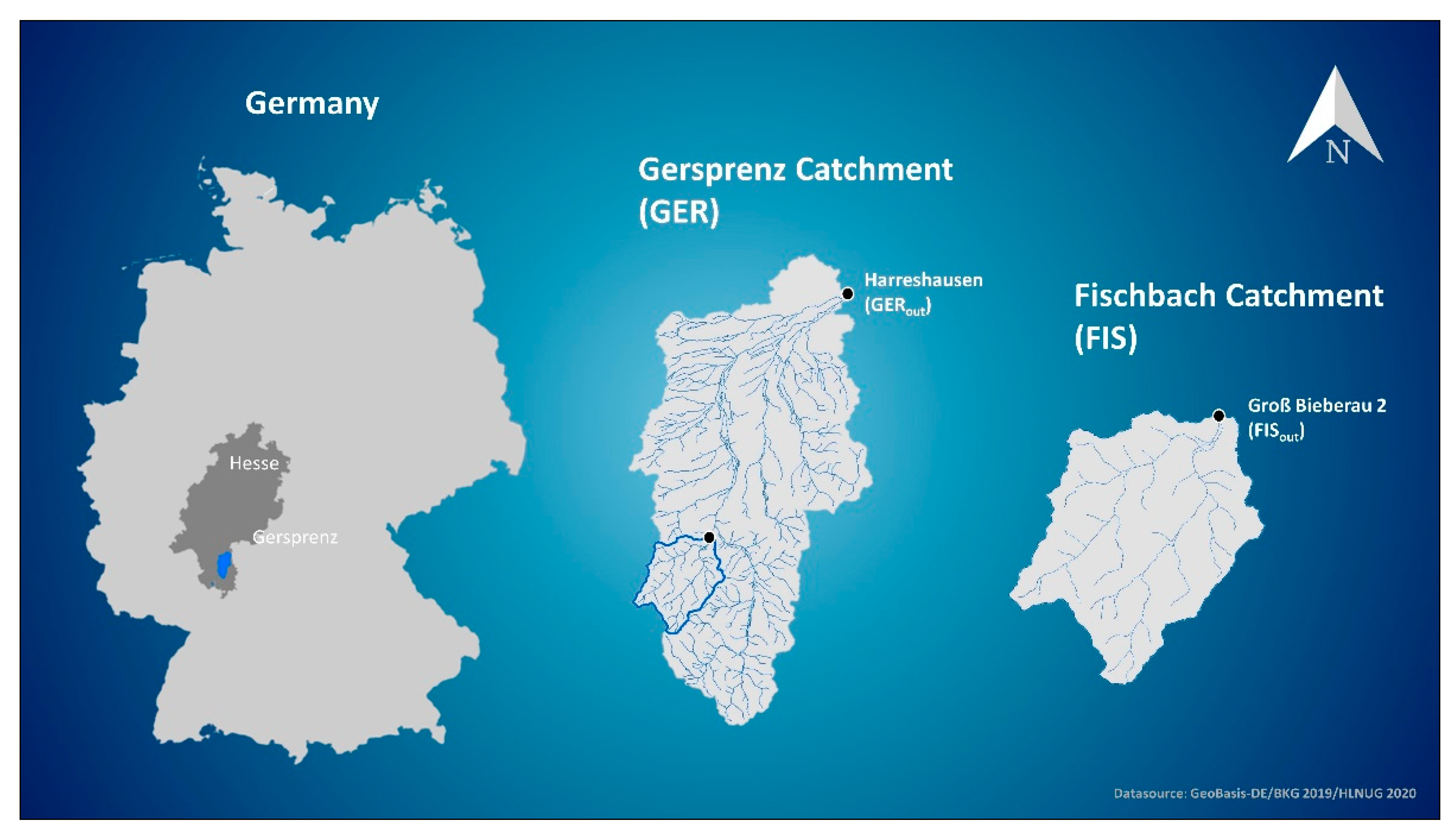
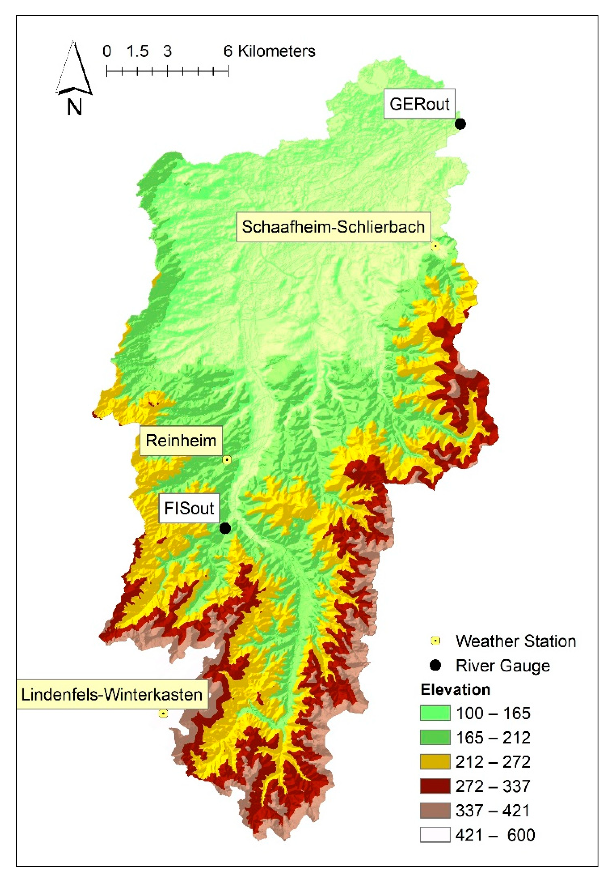
Located in the temperate climate zone of central Europe, the catchment of the Gersprenz river is a typical low mountain range basin. The river basin was established as a field laboratory by the Chair of Engineering Hydrology and Water Management at the Technical University of Darmstadt in 2016 [31], with the goals to enhance the understanding of small-scale catchment processes and to establish an ongoing research with varying foci, creating an integrated and interdisciplinary approach towards hydrological research. The Gersprenz basin measures approximately 500 km², enclosing the significantly smaller subbasin of the Fischbach, which measures approximately 36 km² (Figure 1). The catchment is part of the river basin district Rhine. The Gersprenz river flows into the lower Main river. In agreement with the Water Framework Directive, the Gersprenz may be classified as a “small river” (catchment size between 100 and 1000 km²), while the Fischbach may be classified as a “stream” (catchment size below 100 km²) [32]. As shown in Figure 1, the Gersprenz catchment was delineated by the gauge Harreshausen for this study (ID: 24762653) [33]. The gauge in Groß-Bieberau 2 defines the Fischbach catchment (ID: 24761005) [33].

For simplicity of affiliation, the Gersprenz catchment from now on will be denoted as GER and the Fischbach catchment will be referred to as FIS, while the outlets will be referred to as GER_out and FIS_out, respectively.

The dimensions of the catchments are reflected in the discharge (Q) of the rivers. Within the 39-year study period, a mean discharge ($\overline{Q}$) of 3.08 m³/s was determined for the Gersprenz at the outlet GER_out while $\overline{Q}$ measured 0.34 m³/s at FIS_out, the outlet of the Fischbach (

Table 1. Mean discharge ($\overline{Q})$ and Absolute Minimum Flow (AMF) in the Gersprenz outlet (GER_out) and the Fischbach outlet (FIS_out) for the study period 1980–2018 (data source: The Hessian State Agency for Nature Conservation, Environment, and Geology (HLNUG) [33]).

	GERout	FISout
$\overline{\mathit{Q}}$	3.08 m3/s	0.34 m3/s
AMF	0.37 m3/s	0.02 m3/s

). The lowest recorded daily discharges, the Absolute Minimum Flow (AMF), were 0.37 m³/s and 0.02 m³/s for GER_out and FIS_out, respectively, within the period 1980 to 2018.

In FIS, the elevations range from 160 to 600 m above sea level (m.a.s.l.). GER comprises elevations reaching down to 100 m.a.s.l. The average hill slope in FIS (10.4°) is nearly double the size of the average hill slope in GER (6.2°)—based on a Digital Elevation Model (DEM) of 1 m resolution [34]. The climate changes with varying terrain conditions: The temperature and precipitation data sets retrieved from weather stations in the study region were shown to have distinctive statistical properties, given the different topographical features of the basins. Whilst the average temperature ($\overline{T}$) for the study period measured 10.2 °C in GER, $\overline{T}$ was lower in FIS at 8.8 °C. The average annual precipitation ($\overline{P}$) was 774.8 mm in FIS, whereas GER experienced 641.7 mm of rainfall per year on average for the study period 1980 to 2018 [35]. The climate variable data sets were retrieved from stations in proximity to the gauges. The data should be treated with care, as the stations may not reflect the conditions in the catchment as a whole. The exact locations of the measurement stations are given in the next section.

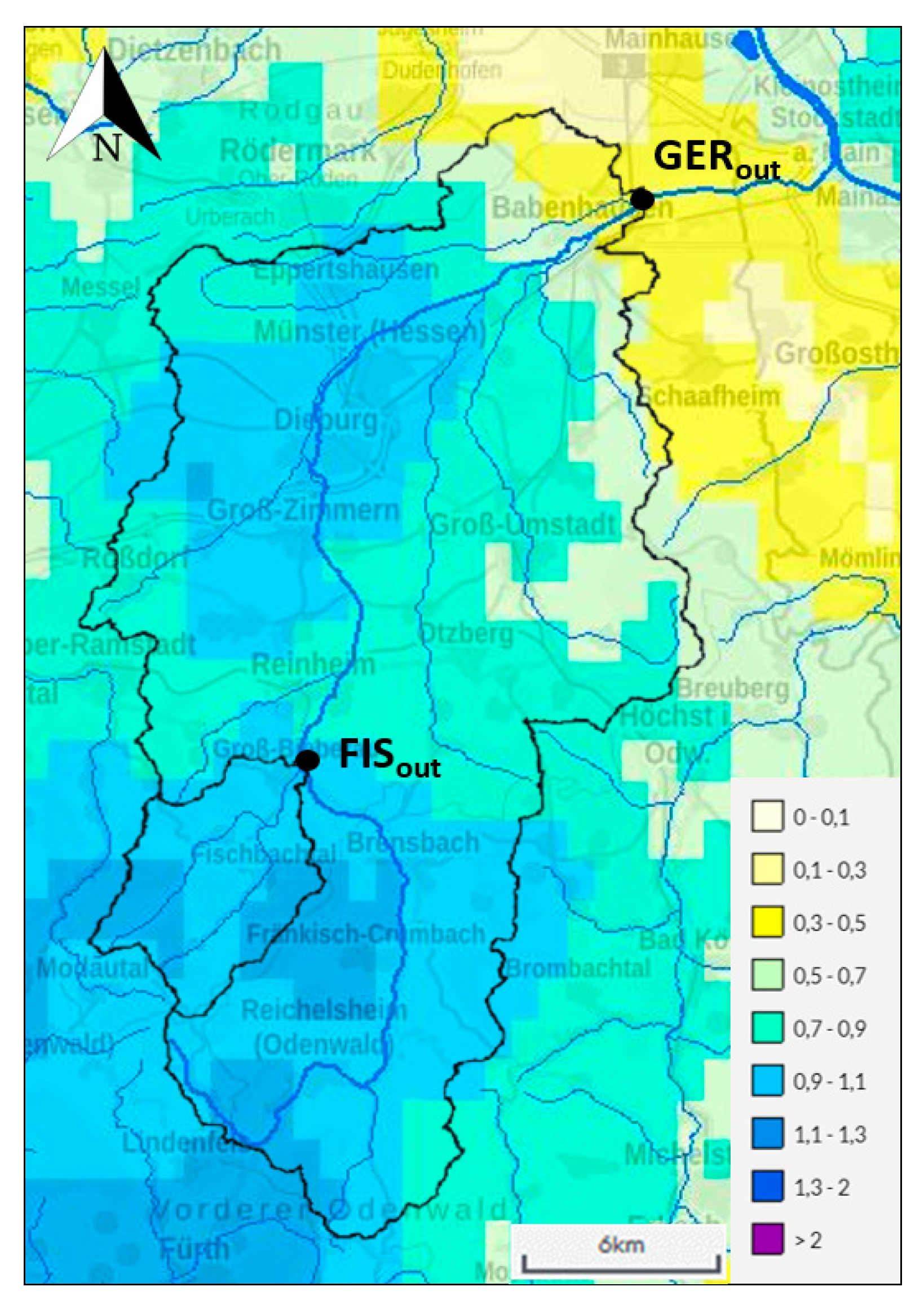
Different drainage densities further characterize the study area GER and its subcatchment FIS. The so-called drainage density defines the ratio between the total length of a river and the catchment area [36]. It is determined by the permeability of the subsoil as well as the slope. High drainage densities indicate steeper slopes than low drainage densities. Furthermore, lower drainage densities in catchments with similar climatic conditions indicate higher permeability of subsoils and deep seepage. The drainage density in FIS was shown to be slightly higher than in GER (compare Figure 2), indicating that, in FIS, impermeable soils may prevail while reflecting the sloping terrain of the subcatchment.

In general, FIS is a typical German low mountain range river basin dominated by coarse substrates and rich in silicates. Different forms of granite and diorite prevail in this area, which is part of the crystalline Odenwald [37]. Thus, the water storage capacity in FIS is presumably low. To the north, the catchment area of the Gersprenz passes from the crystalline Odenwald to the Reinheimer Hügelland (Reinheimer Hill Country) into the Untermainebene (lower Main plain). Soft rock soils made of sand, gravel, and clay dominate here. The Untermainebene consists mostly of tertiary deposits covered by younger river deposits [31]. Consequently, the lower areas of GER are characterized by higher infiltration rates and water storage capacities.

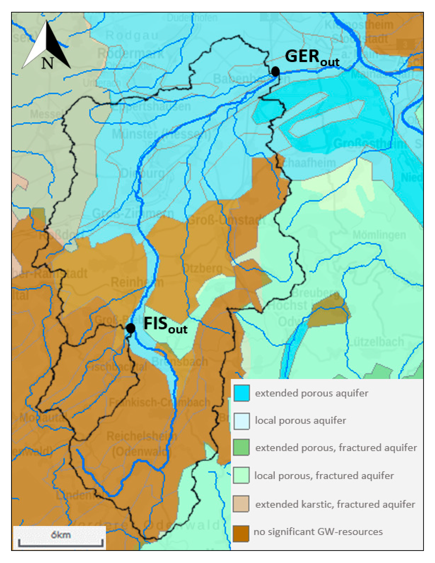
The groundwater (GW) resources reflect this: large parts of the study area go without any significant GW reservoirs. However, an extended porous aquifer is located in the subsurface north of GER (See Figure 3). This leads to a higher overall yield in the wells in the northern part of the catchment. The yield of the wells in FIS is estimated to be less than 2 L/s [38]. While the GW reserves vary noticeably between the northern and southern parts of the study region, the GW recharge rates were shown to be nearly equal in GER and FIS. The Federal Institute for Geosciences and Natural Resources (BGR [39]) estimated average, annual GW recharge rates for Germany based on a multi-level regression method [40]. Based on this data, the average annual GW recharge rates were found to be 134 mm/a and 140 mm/a in FIS and GER, respectively. In agreement with the Bavarian State Office for the Environment (LfU), GW recharge should not be set equal to the GW availability [41]. Especially the crystalline, mountainous areas are often characterized by high GW recharge rates but low underground storage capacities.

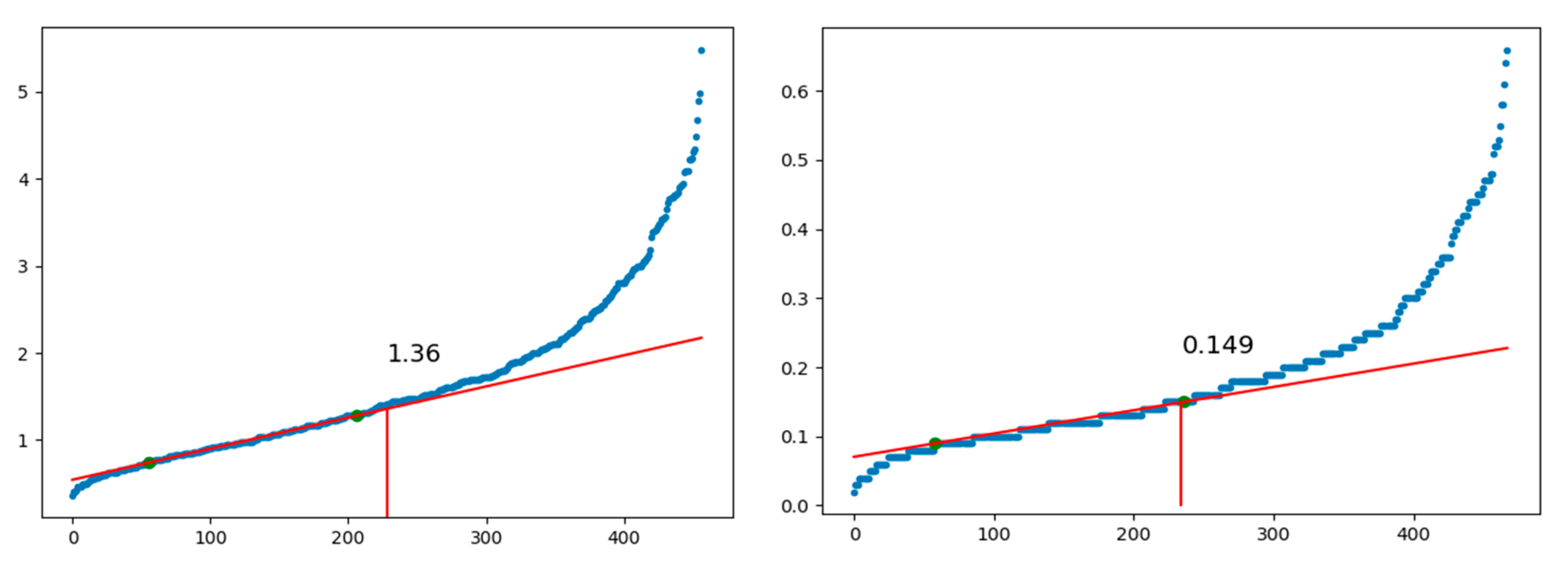
On the scale of annual values, the groundwater recharge rate corresponds approximately to the baseflow, which feeds the receiving water body even during periods of low rainfall. Thus, the baseflow is the fraction of the GW feeding into the river, which may be indicated by the Baseflow Index (BFI) [42]. Kissel and Schmalz [43] investigated the suitability of various baseflow estimation methods for German low mountain ranges based on the discharge time series retrieved from FIS_out. The examined baseflow separation methods included digital filters, a Mass Balance Filter (MBF), and noncontinuous estimation methods. Based on the results of the conducted analysis, a recommendation to use the Kille method for baseflow estimation was derived for the study region. Consequently, this method was applied to estimate the BFI for GER_out and FIS_out. The plot of the ranked monthly minima from 1980 to 2018 is shown for the respective river gauges in Figure 4.

The mean baseflow in GER_out is 1.36 m³/s, which corresponds to a BFI of 0.44. The mean baseflow in FIS_out is 0.149 m³/s, resulting in a BFI of 0.45. The BFI in FIS_out deviates by 0.01 from the BFI detected by Kissel and Schmalz for the same river gauge. This may be explained by the different study periods; Kissel and Schmalz [43] determined the BFI based on daily discharge data from 1974 to 2013, while in this study, the computation was based on daily discharge data from 1980 to 2018.

Additional discharge into the Gersprenz takes place through municipal wastewater treatment plants at nine locations. The inlets are located mostly close to settlements. In FIS, no additional water is discharged into the stream [45]. Anticipating that the additional discharge in GER was not taken into consideration in the determination of the BFI, the baseflow fraction in FIS_out is estimated to be slightly higher than in GER_out, despite the lower storage capacity of the crystalline Odenwald.

It is common knowledge that hydrological processes are greatly influenced by land-use [46]. An analysis of the change layers of the CORINE Land Cover data set [47] showed that no significant increase in sealed soil took place between 1990 to 2018 (reference year) in the study area. Paved areas were augmented by approximately 2%. According to Authorative Topographic-Cartographic Information System (ATKIS) data provided by the Hessian Agency for Land Management and Geoinformation (HVBG [34]), GER is dominated by agricultural land-use types, which add up to 48.3%. Forests are ranked second with 36.1%, while settlements make up 12.6% of the land-use coverage. In FIS, the prevailing land-use type is forests, with 50.1%. Agriculture and settlements take up 41.8% and 6.5% of the area, respectively (See Schmalz and Kruse [31] for a more detailed description of land-use types in the research basin). Consequently, water resources in the entire Gersprenz catchment are mainly used for agricultural purposes. However, extractions for private purposes are also notably high and have become an issue during dry periods, as repeatedly reported by local newspapers (e.g., ECHO) [48]. In 2018, the low flow situation reached a point to which the regional council of Darmstadt imposed restrictions on water withdrawal due to the alarming water scarcity [49].

2.2. Database

Historic low flow and drought analyses require long-term, consistent measurement time series. The discharge measurement data used in this study was provided by the HLNUG as daily averages for the stations GER_out and FIS_out for the entire study period 1980–2018 [33].

The measurements of climate variables T and P were retrieved from measurement stations of the German weather service (DWD) [35]. Available data was highly limited due to the period of interest being only 39 years. Finally, with the objective to link the climate variables to the discharge measurements, the weather stations were selected according to their proximity to the gauges. P for the catchment of Fischbach was retrieved from the station Reinheim, located at 165 m.a.s.l., as shown in Figure 5. Unfortunately, the station Reinheim (ID: 4134) lacked T records.

Time series on T were retrieved from the weather station Lindenfels-Winterkasten (ID: 3018), which is located at 445 m.a.s.l. and was found to be representative for the subcatchment.

The weather station closest to GER_out was found to be Schaafheim-Schlierbach (ID 4411), providing both P and T time series. This station is located at 155 m.a.s.l., and was therefore representative for the elevation range of 100 to 165 m.a.s.l. (compare Figure 5). Missing values were interpolated via regression analysis.

2.3. Drought Indices

Studies have shown that there is a close interrelation between the occurrence of droughts and the variability of T and P over time [50,51,52,53]. Changes in P patterns and increasing T were shown to favor the emergence of droughts. Therefore, this study initially observed the trends and development of annual average T and annual sums of P in the study region. Subsequently, the occurrence of droughts throughout the study period was investigated. In order to adequately identify and classify the severity of drought events, existing indices were used. In agreement with the German Weather Service [54], the Standardized Precipitation Index (SPI) is the most widely used drought index. Developed by McKee et al. [55], the index enables classification of drought according to its magnitude while expressing the drought event’s probability (

Table 2. Standardized Precipitation Index (SPI) and Standardized Precipitation-Evapotranspiration Index (SPEI) categories and their probability of recurrence.

Range	Category	Probability of Recurrence
−1 to 0	mild dryness	1 in 3 years
−1.5 to −1	moderate dryness	1 in 10 years
−2 to −1.5	severe dryness	1 in 20 years
≤−2	extreme dryness	1 in 50 years

). The index may be calculated based on multiple timescales reflecting the impacts of a drought on various water resources [56].

In this study, the SPI was obtained for each calendar year by fitting a gamma distribution to monthly precipitation values. For an automated computation of the index, the R-Studio package precincton (precipitation intensity, concentration, and anomaly analysis) was used [57]. The advantage of the SPI index requiring only P data in its computation is also its offset. Especially with climate change and increasing global temperatures [58], it has become of interest to include evaporation processes as a factor in the identification of drought events. Thus, an extension of the SPI was developed by Vicente-Serrano et al. [59], namely the Standardized Precipitation-Evapotranspiration Index (SPEI). The SPEI takes into consideration Potential Evapotranspiration (PET) in mm based on T time series and the measurement location. Based on the limited data availability, Hargreaves’ equation was chosen for the determination of PET:

$$ET=0.0022\ast R_A\ast \mathsf{\Delta }{T}^{0.5}\ast \left(T+17.8\right),$$

(1)

where $R_A$ is the mean extraterrestrial radiation (mm/a), which is a function of the latitude; $\mathsf{\Delta }T$ is the temperature difference of the mean monthly maximum temperature and the mean monthly minimum temperature for the respective month of interest (°C); and $T$ is the mean air temperature (°C) [60]. The SPEI was computed using the R-Studio package SPEI developed by Čadro and Uzunović [61] for each calendar year of the study period. Both indices were obtained taking into account 3-, 6-, 12-, and 24 months of antecedent rainfall. Therefore, the minimum requirement of 30 years for good results was exceeded [62]. Based on the analysis of T, P, SPI, and SPEI time series, it was possible to depict exceptionally dry years, so-called drought years, within the study period.

2.4. Low Flow Indices

According to German normative regulations, low flow may be defined as a minimum flow that falls below a certain threshold (DIN4049) [63]. The thresholds thereby applied are based on the averages of so-called n-day time series [6,64]. In this study, the 1-, 7-, and 30-day annual minima (AMIN, AMIN7, and AMIN30) were determined [65,66]. In order to ensure comparability with the drought indices, all low flow indices were computed for each calendar year of the study period. The n-day time series showed the development of the lowest daily, weekly, and monthly flows for each year of the study period 1980–2018, consisting of 39 flow rates given in m³/s. The time series were analyzed for trends as described in the last subsection of this section. The threshold values were calculated based on the n-day time series. In detail, they were derived by creating the mean of the annual minima time series (MAM, MAM7, and MAM30) [21]. Based on these thresholds, it was possible to determine the characteristic values SumD, MaxD, and SumV (see

Table 3. Low flow characteristic values [67].

Characteristic Value	Description	Unit
SumD	Total number of days within a year on which the flow falls below a defined threshold.	Days (d)
MaxD	Maximum number of consecutive days within a year on which the flow falls below a defined threshold.	Days (d)
SumV	Sum of the volumetric deficit between the daily flow and a defined threshold for one year.	Volume (m3)

).

These further values enabled us not only to take into account the absolute minima, as given by the n-day time series but also to identify the frequency and duration of low flow events. While SumD defines the total number of days with flow under a certain threshold, MaxD describes the maximum number of consecutive days with low flow for each year. If the difference between the two parameters is minor, the longest continuous period of low flow is regarded as characteristic for the respective year [9]. SumV is the volume deficit in m³ for each year. As SumV is an absolute number, which is linked to the stream size, a fourth threshold-dependent indicator was determined: MAM7-days is the number of days with MAM7 flow needed to balance out the deficit of each year [9]. Finally, consulting these indicators, it was possible to identify the years especially effected by low flow and to link these with the prior determined drought years. In addition, the development of the characteristic values throughout the investigative period was examined for trends.

Finally, low flow is significantly influenced by the catchment’s water storage capacity. High storage capacities will buffer meteorological extremes [68]. The ratio MAM/$\overline{Q}$ indicates the storage capacity of a catchment as well as the variability of the discharge regime throughout the year [9]. The index ranges between 0 and 1, and the higher the value of the index, the lower the sensitivity of a catchment towards hydrological extremes, such as droughts.

As mentioned, the calculation of low flow extremes and characteristic values was executed based on historical measurement data retrieved from the gauges GER_out (delineating the Gersprenz catchment) and FIS_out (delineating the Fischbach catchment) [33]. The period for the study (1980–2018) was chosen according to data availability while ensuring that the total amount of years taken into consideration exceeded the minimum requirement for the low flow statistical analysis of 30 years [21,67].

2.5. Trend Analysis

The trend analyses in this study were carried out according to the regulations of the German Association for Water, Wastewater, and Waste [69,70]. Trends were depicted for the measurement time series as well as the obtained drought and low flow indices for the study period 1980 to 2018 using a simple linear regression analysis. The significance of the trends was evaluated with Student’s t-test at a significance level of 5% (α = 0.05) after confirming a normal distribution of the respective data set using the Kolmogorov–Smirnov Test.

3. Results

3.1. Temperature and Precipitation

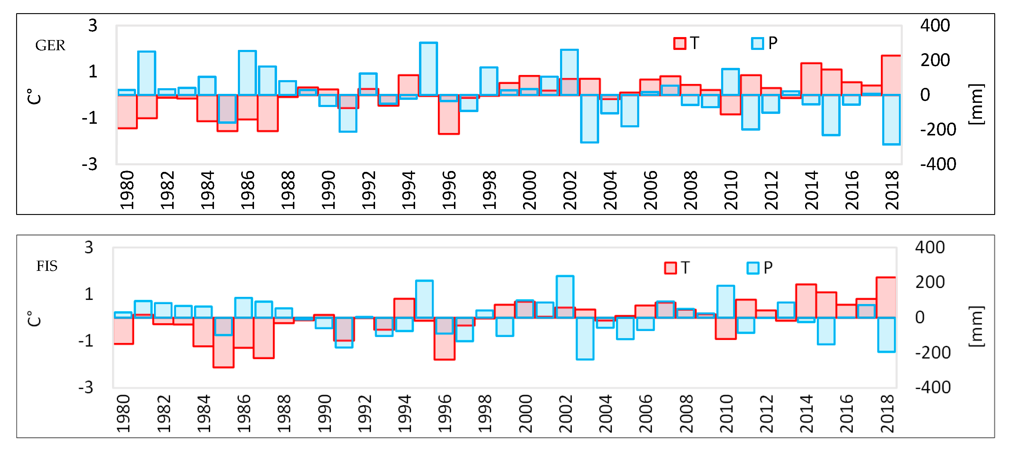
Average annual T was shown to significantly increase throughout the study period. As measurement data on evaporation was not available for the study region [71], total annual PET was obtained using the Hargreaves method (see the section on drought indices). The results displayed a significant increase in the determined annual PET in the study area from 1980 to 2018. The average PET in FIS was 730 mm for the study period, increasing by 2.7 mm per year. In GER, the average annual PET was nearly 843 mm, with an increase of 3.7 mm each year. The increases in T and PET are likely to be affiliated with climate change, as supported by the global analysis given in the National Center for Environmental Information’s Global Climate report (NOAA) [72] as well as a regional analysis conducted by the Hessian Center for Climate Change and Adaptation [10]. While the increase in global T is quite certain, the resulting effects of climate change on P are harder to measure and predict due to regional and seasonal variations in rainfall patterns [73]. This was confirmed by the results of this study, where a negative trend of total annual rainfall was examined in both catchments but only the decline of annual P in FIS was shown to be significant at the 95% confidence level. Dry years were identified by observing deviations from the long-term averages (N = 39 years). The five years with a maximum sum of the absolute positive deviations of $\overline{T}$ and the absolute negative deviations of $\overline{P}$ were classified as exceptionally dry for both catchments, with 2018, 2015, 2011, 2003, and 1991 resulting as dry years (Figure 6).

The identified dry years correspond to the dry years defined in Klimaveränderung und Wasserwirtschaft (KLIWA)—a study on low flow carried out by the south German states Baden-Wuerttemberg, Rhineland-Palatinate, and Bavaria [9]. The findings confirm that 2018 was an extremely hot and dry year [11,29]. The results should be treated with care, as uncertainties arise from the locations of the historic weather stations, which are in the lower areas of the respective catchments and do not take into account rainfall events in the upper elevations of the catchments [74].

3.2. Drought

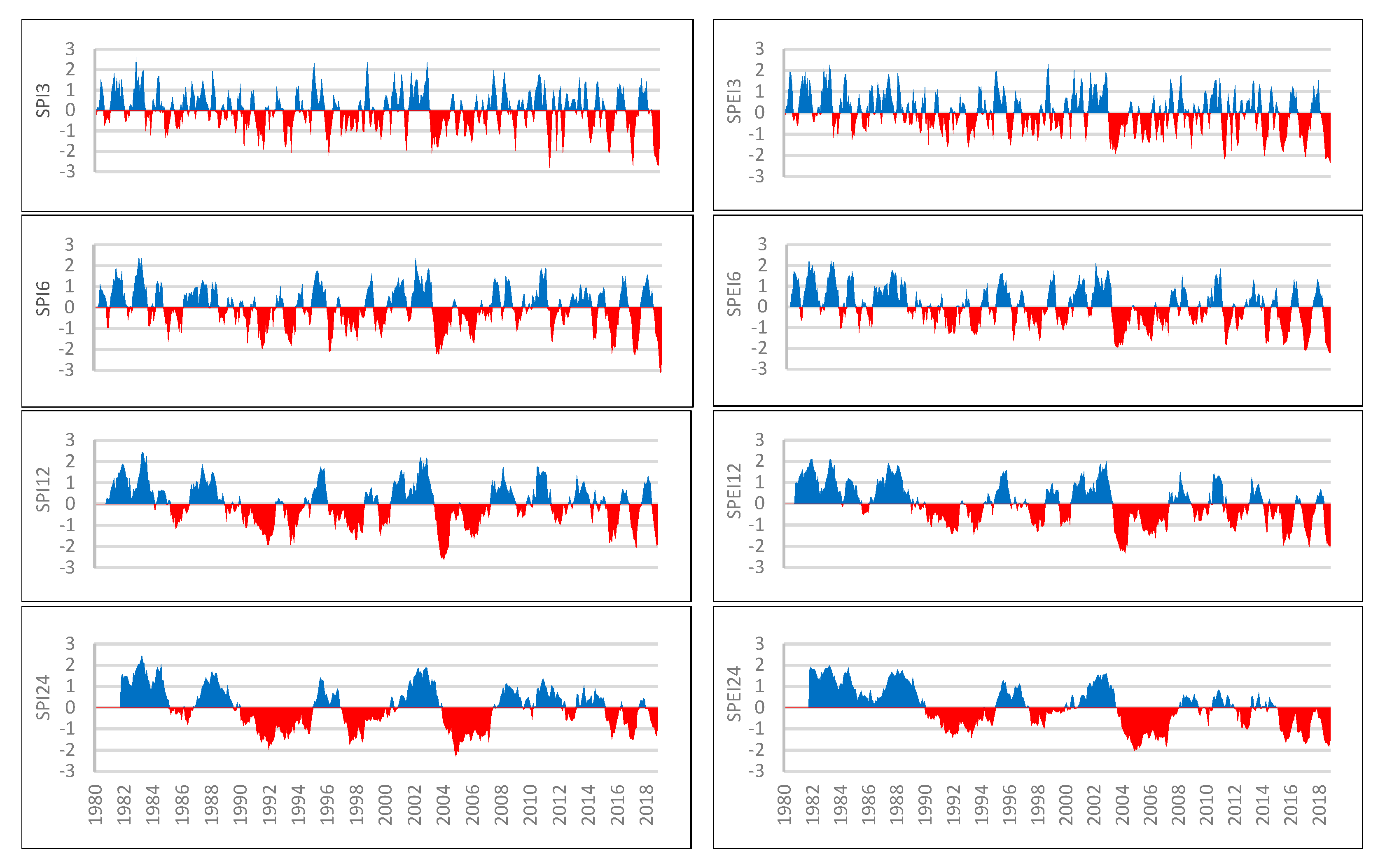
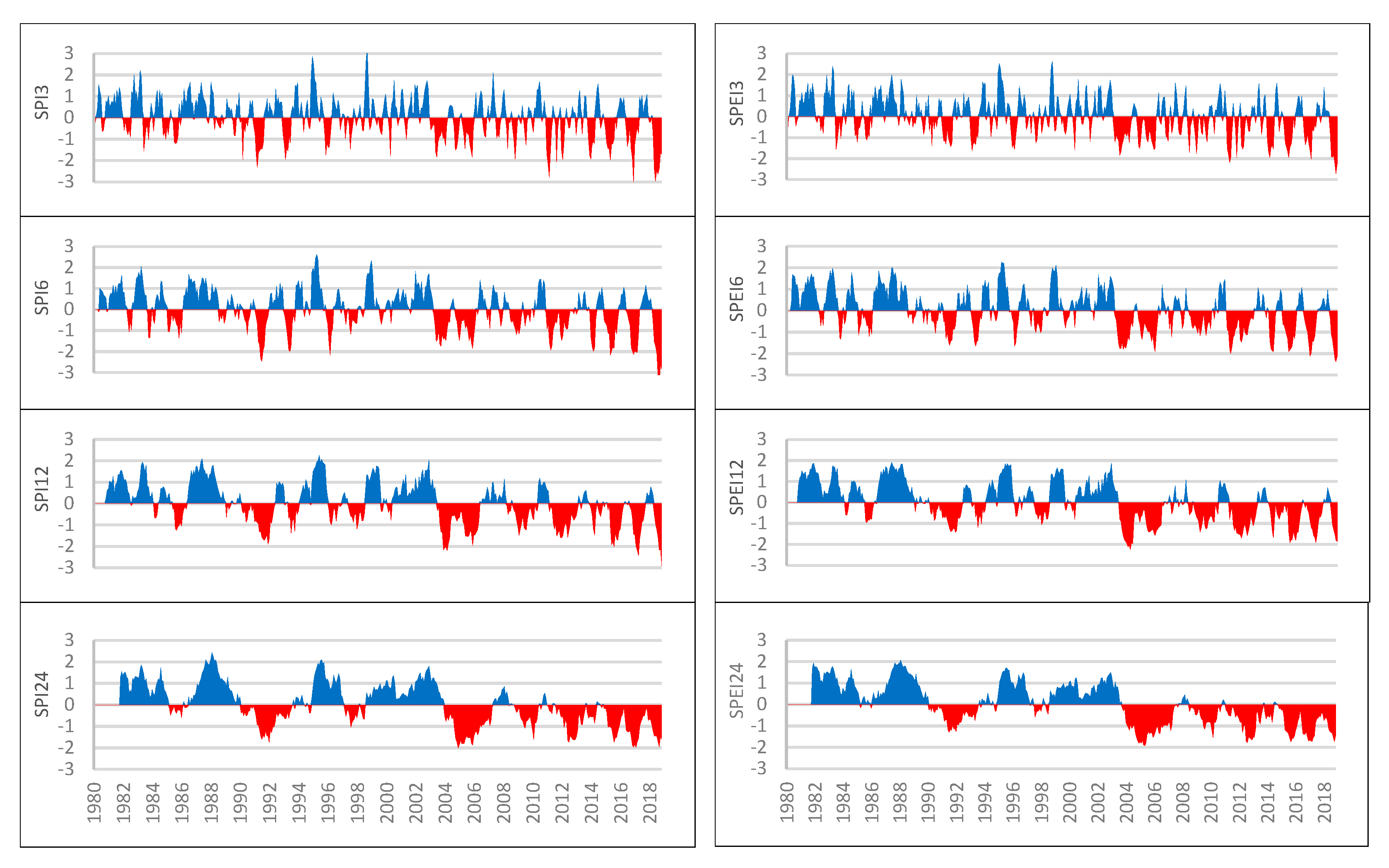
The number of months considered in the calculation of drought indices determines the drought characteristics [56,75]. SPI3 and SPEI3 take into consideration three months for each monthly index and therefore reflect short-term P patterns. HLNUG [29] states that the SPI3 indicates agricultural droughts in Germany. Taking into account more months within the calculation process will indicate medium- to long-term changes in P, which are likely to affect changes in the hydrological realm. Considering 6 months for the calculation will indicate seasonal trends in P, determining stream flow and reservoir levels, while taking into account 12 or more months will designate drought events, which may even hint to changes in GW levels [56]. Figure 7 and Figure 8 show the drought indices SPI and SPEI for 3-, 6-, 12-, and 24 months throughout the study period for GER and FIS, respectively.

The SPI24 and SPEI24 take into consideration many months, usually resulting in the minor fluctuations in wet and dry conditions balancing out to zero, which is why these indices designate historically exceptional droughts [56]. Observing the results in Figure 7 and Figure 8, it is remarkable to see a shift from predominantly moist conditions, which are indicated by positive SPI24 and SPEI24 values in blue, to predominantly dry conditions, indicated by the negative values in red, in both catchments. In general, the results presented in Figure 7 and Figure 8 confirm the findings of Bindi et al. [62] and Labudová et al. [75], which state that, with an increasing number of months, drought events will become less frequent with longer durations and lower magnitudes.

Extreme events with indices lower than -2 usually occur once every 50 years [56]. The findings presented in

Table 4. Years with extreme drought events (SPI and SPEI ≤ −2 and a probability of recurrence of 1 in 50 years) taking into consideration the 3-, 6-, and 12-month antecedent conditions in GER and FIS.

		SPI			SPEI
RK		3	6	12	3	6	12
GER	1	2011 (May)	2018 (Oct–Dec)	2004 (Jan–Jul)	2018 (Jul–Nov)	2018 (Sep–Dec)	2004 (Jan–May)
	2	2017 (Jan–Feb)	2017 (Jan–Feb, Apr)	2003 (Dec)	2011 (May–Jun)	2017 (Jan–Mar)	2017 (Jun)
	3	2018 (Aug–Nov)	2003 (Jul–Sep, Nov)	2017 (Jun)	2017 (Feb)	2003 (Aug–Sep)	2018 (Dec)
	4	1996 (Mar)	2015 (Jul)		2014 (Mar)		2003 (Dec)
	5	2003 (Apr)	1996 (Mar–Apr)		2011 (Jun)
	6	2012 (Apr)
	7	2015 (Jun–Jul)
	8	1993 (Aug)
FIS	1	2016 (Dec)	2018 (Aug–Dec)	2018 (Oct–Dec)	2018 (Oct–Dec)	2018 (Oct–Dec)	2004 (Mar–May)
	2	2018 (May–Sep)	1991 (Jul–Aug)	2017 (Mar–May)	2011 (May)	2017 (Jan)
	3	2011 (Feb–Mar, Sep)	2015 (Jun)	2004 (Jan–Apr)	2017 (Feb)	2011 (Jun)
	4	1991 (Apr)	1996 (Apr)	2015 (Sep)
	5		2017 (Jan, Mar–Apr)

display the years and month(s) in which extreme drought events took place in GER and FIS throughout the study period 1980 to 2018. Extreme events were determined when the indices SPI3, −6 and −12, as well as SPEI3, −6 and −12, fell below -2. They were ranked according to their magnitude. More than 92% of extreme events occurred in the last 15 years of the 39-year study period.

With respect to the indices, it was shown that, when taking into account PET in drought determination, as done for computation of the SPEI, the magnitudes of the events were considered less extreme, as the total number of extreme events detected with the SPEI was lower than that of the SPI. Computation of the SPI and SPEI on the 6- and 12-month bases showed an increase in the magnitude of hydrologically relevant droughts. It was shown that the magnitudes of the drought events significantly increased at the 95% confidence level throughout the study period in both catchments. The years dominated by droughts with high magnitudes and long durations were found to be coherent with the dry years depicted in the last section of this paper. Regarding the magnitude and duration of drought, 2018 was shown to be an exceptional year.

3.3. Low Flow

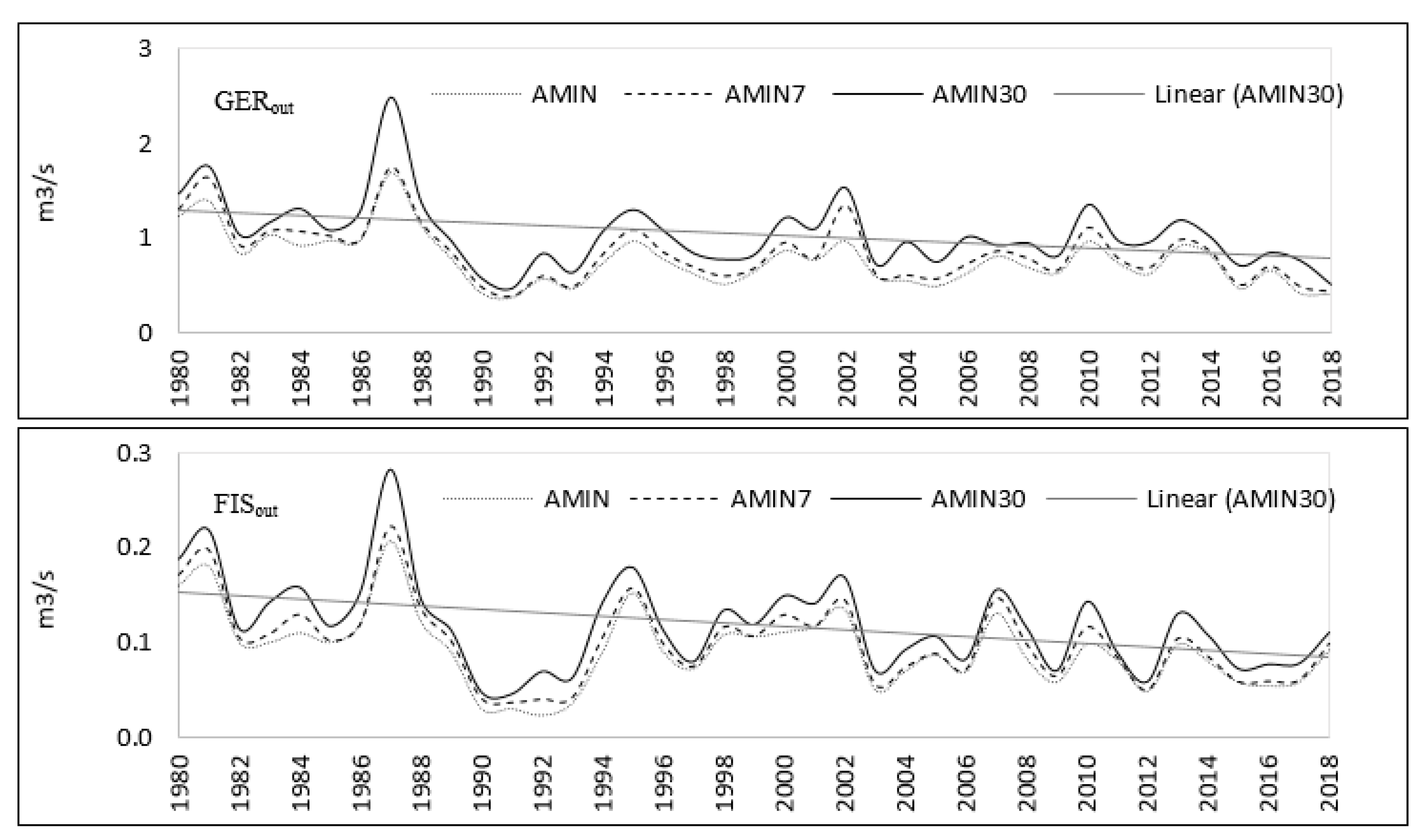
Annual $\overline{Q}$ significantly decreased throughout the study period at both gauges (t-test). A slight decrease in annual maxima was observed but was not found to be significant at the α = 0.10 level after accounting for serial correlation. The time series of AMIN, AMIN7, and AMIN30 displayed significant negative trends at both gauges (Figure 9). The results confirm a decline in water availability in the Gersprenz and Fischbach catchments from 1980 to 2018. The findings are supported by the study conducted by KLIWA, which states that climate trends, such as increasing T, have a greater impact on low flow than on average flow [9].

The five years with the lowest AMINx values and the year and month(s) of occurrence are ranked in

Table 5. Top five years with the lowest extreme values (AMIN, AMIN7, and AMIN3) in GER_out and FIS_out.

	GERout			FISout
RK	AMIN	AMIN7	AMIN30	AMIN	AMIN7	AMIN30
1	1991 (Sep)	1991 (Sep)	1991 (Aug/Sep)	1992 (Sep)	2017 (Jun)	1991 (Aug/Sep)
2	1990 (Aug)	2018 (Sep)	2018 (Aug/Sep)	1990 (Jul)	1991 (Sep)	1990 (Jul/Aug)
3	2017 (Jun)	1990 (Aug)	1990 (Jul/Aug)	1991 (Aug)	1990 (Jul/Aug)	2017 (May/Jun)
4	2018 (Sep)	1993 (Aug)	1993 (Aug/Sep)	2017 (Jun)	1992 (Sep)	2012 (Aug/Sep)
5	1993 (Jul)	2017 (Jun)	2015 (Aug/Sep)	1993 (Jul)	1993 (Jul)	1993 (Jun/Jul)

. Most extreme values occurred in the late summer months or in the early autumn months. This confirms the findings of Belz et al. [76].

In addition, it was shown that the years 1990–1993 were determined by extreme low flows in both catchments. The analysis of T and P data identified 1991 as a dry year. However, dry conditions ranging over a period of three years were not immediately visible. From the drought indices, the SPI and SPEI24 clearly depicted this period as exceptionally dry, showing that antecedent drought conditions play a major role when dealing with low flow.

In general, extreme AMINx values do not reflect the duration of low flow events and the frequency of low flows throughout the year. This is why further low flow characteristic values were determined. By averaging the n-day time series, it was possible to obtain the threshold values necessary for determination of the characteristic values SumD, MaxD, and SumV (

Table 6. Threshold values retrieved by averaging the AMIN, AMIN7, and AMIN30 time series.

	GERout	FISout
MAM	0.772 m3/s	0.093 m3/s
MAM7	0.851 m3/s	0.102 m3/s
MAM30	1.043 m3/s	0.118 m3/s

).

Characteristic values were given for the thresholds MAM, MAM7, and MAM30 for each year of the study period. The threshold MAM was obtained by averaging the AMIN time series, the threshold MAM7 was obtained by averaging the AMIN7 time series, and so on. It may be pointed out that, with an increasing number of days taken into account for calculation of the threshold, the resulting characteristic values are augmented: e.g., the total number of days with low flow for the study period will be higher for the monthly threshold MAM30 than for the daily threshold MAM.

The results are presented in

Table 7. Characteristic values GER_out 1980–2018.

	SumD (d)			MaxD (d)			SumV (m3)
Threshold	MAM	MAM7	MAM30	MAM	MAM7	MAM30	MAM	MAM7	MAM30
1980	0	0	0	0	0	0	0	0	0
1981	0	0	0	0	0	0	0	0	0
1982	0	1	15	0	1	13	0	953	120,849
1983	0	0	3	0	0	2	0	0	842
1984	0	0	3	0	0	3	0	0	16,394
1985	0	0	34	0	0	10	0	0	30,277
1986	0	0	9	0	0	7	0	0	28,446
1987	0	0	0	0	0	0	0	0	0
1988	0	0	0	0	0	0	0	0	0
1989	0	6	50	0	1	13	0	13,492	497,871
1990	59	82	103	25	33	45	724,098	1,208,226	2,707,303
1991	102	112	142	33	40	48	1,786,486	2,524,165	4,592,263
1992	24	45	89	8	10	25	172,534	407,476	1,537,839
1993	63	88	148	21	21	25	855,958	1,347,862	3,347,195
1994	1	7	56	1	3	15	2725	25,676	458,946
1995	0	0	4	0	0	2	0	0	11,490
1996	1	8	41	1	2	11	133	18,853	426,225
1997	18	30	70	6	12	24	106,937	260,130	1,082,363
1998	27	36	65	17	18	22	223,045	438,646	1,298,688
1999	13	26	70	9	17	26	57,888	177,696	1,061,627
2000	0	0	13	0	0	6	0	0	102,144
2001	3	9	24	2	7	9	399	38,814	335,055
2002	0	0	1	0	0	1	0	0	6329
2003	22	36	89	9	11	30	222,380	408,406	1,441,935
2004	10	13	45	10	10	14	103,281	176,544	601,876
2005	68	91	132	17	19	31	654,447	1,181,376	3,018,705
2006	15	22	56	6	7	22	63,338	189,438	863,298
2007	0	5	28	0	2	16	0	6491	316,305
2008	10	32	74	3	8	10	28,977	169,588	1,020,414
2009	34	44	78	15	18	20	172,999	441,083	1,472,544
2010	0	0	3	0	0	3	0	0	18,122
2011	4	14	109	2	8	41	6580	60,857	993,083
2012	11	23	62	7	9	16	56,758	165,334	862,390
2013	0	0	15	0	0	6	0	0	75,057
2014	0	6	31	0	3	19	0	4852	328,379
2015	94	109	138	22	25	33	906,735	1,612,379	3,682,213
2016	23	39	67	9	11	13	65,265	285,120	1,131,633
2017	47	64	88	17	18	18	547,975	914,599	2,168,278
2018	116	127	148	39	45	47	1,872,155	2,706,934	4,972,379
Total	765	1075	2103	279	359	646	8,631,094	14,784,990	40,628,758
Trend	sig.	sig.	sig.	sig.	sig.	sig.	-	-	sig.

and

Table 8. Characteristic values FIS_out 1980–2018.

	SumD (d)			MaxD (d)			SumV (m3)
Threshold	MAM	MAM7	MAM30	MAM	MAM7	MAM30	MAM	MAM7	MAM30
1980	0	0	0	0	0	0	0	0	0
1981	0	0	0	0	0	0	0	0	0
1982	0	4	23	0	2	9	0	618	20,323
1983	0	1	10	0	1	7	0	154	8198
1984	0	0	1	0	0	1	0	0	733
1985	0	17	24	0	5	12	0	2626	32,289
1986	0	0	0	0	0	0	0	0	0
1987	0	0	0	0	0	0	0	0	0
1988	0	0	0	0	0	0	0	0	0
1989	3	13	37	1	3	8	658	4600	40,959
1990	84	101	113	49	53	54	194,679	264,431	418,966
1991	133	152	162	73	74	75	345,394	454,611	681,269
1992	81	100	109	28	29	29	151,685	219,348	370,241
1993	89	132	155	26	41	42	182,816	260,579	467,912
1994	3	5	13	3	3	7	658	3364	16,446
1995	0	0	0	0	0	0	0	0	0
1996	2	10	35	2	3	12	439	3272	36,036
1997	51	63	85	25	32	33	38,833	81,442	188,480
1998	0	0	2	0	0	2	0	0	1467
1999	0	0	15	0	0	13	0	0	11,000
2000	0	0	1	0	0	1	0	0	733
2001	0	0	0	0	0	0	0	0	0
2002	0	0	0	0	0	0	0	0	0
2003	67	83	113	26	27	37	97,639	153,651	295,414
2004	81	99	118	28	29	29	45,413	112,922	269,705
2005	13	23	49	8	10	12	2851	14,784	67,039
2006	47	83	95	19	23	40	37,092	80,211	208,774
2007	0	0	0	0	0	0	0	0	0
2008	4	20	46	2	4	9	1741	7409	55,335
2009	63	101	139	20	49	73	66,521	122,735	296,338
2010	0	1	5	0	1	2	0	154	4531
2011	72	143	176	27	45	45	18,383	86,885	317,424
2012	95	134	170	52	66	69	150,436	232,375	452,128
2013	0	3	17	0	3	10	0	463	15,059
2014	19	29	47	6	8	10	9351	26,079	81,124
2015	85	117	157	27	50	79	108,585	188,364	385,398
2016	0	2	26	0	2	6	0	1000	20,364
2017	109	128	173	24	24	39	292,437	388,783	609,676
2018	53	88	139	22	29	30	60,008	120,554	289,080
Total	1154	1652	2255	468	616	795	1,805,620	2,831,417	5,662,441
Trend	-	sig.	sig.	-	-	sig.	-	-	-

. A color scale was adapted ranging from green (low values) to red (high values). The sums of the characteristic values for the 39-year study period are given below the time series in the second-last row of the table. Whether the detected trends of each annual time series are significant at the 95% level is indicated in the last row.

Significant increases in SumD and MaxD were identified for all MAMx thresholds in GER_out (Table 7), indicating a tendency towards years with more days with discharge subceeding the threshold as well as a prolongation in the duration of low flow periods. For the characteristic value SumV, increasing trends were detected; however, the trend was only significant at the 95% level with a threshold of MAM30. In FIS_out, positive trends were equally identified for all characteristic values. For SumD, these were only significant with MAM7 and MAM30 as thresholds, whereas the development of MaxD over time showed only a significant positive trend with MAM30 as the threshold (Table 8). For SumV, no significant trends were detected in FIS_out. Interesting enough, when observing the characteristic values, close to double the number of total SumD and MaxD values were found in FIS_out compared to GER_out. This exposes FIS_out as far more likely to experience low flows of higher frequencies and durations compared to GER_out. In contrast, GER_out displays significant increases in SumD and MaxD already at the lowest threshold.

Prior dry years were identified based on annual T and P deviations as well as drought intensities within that year. The years with high SumD and MaxD values indicated the years with exceptionally many days with low flow and long low flow durations. In GER, these low flow years correspond better to the dry years than in FIS. A clarifying example is given in the extreme year 2018: this year was the most extreme year regarding droughts, identified by the drought indicators SPI and SPEI. On the one hand, this is reflected by the characteristic values in GER_out, where 2018 is the most extreme low flow year for each category and threshold. On the other hand, low flow in FIS_out seems to have been less affected by the intense hot and dry period in 2018. As an extreme low flow year, the year 1991 stands out in FIS_out.

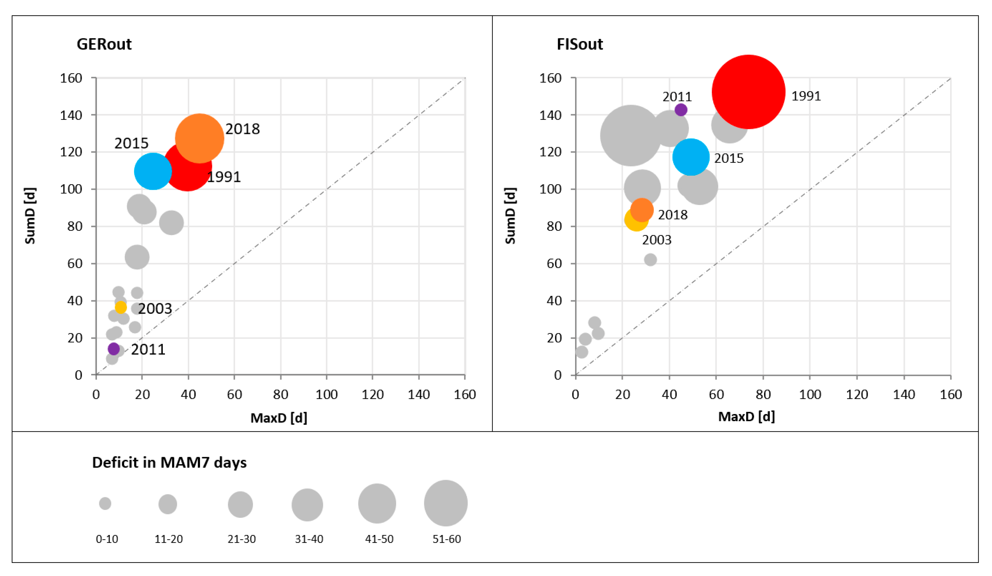
These results are further visualized in Figure 10, where SumD and MaxD are presented as scatterplots for each catchment for the threshold MAM7. Each year is indicated as a point value within the scatterplot. The closer the points are to the dotted line, the larger the fraction of consecutive days with low flow within that year. A point located on the dotted line indicates a year with an uninterrupted low flow event. The size of each dot indicates the number of days needed to balance out the deficit within that year. The larger the circle, the more days with MAM7 flow needed to compensate the lack of water. While GER would have needed 37 days of MAM7 flow to balance the deficit in 2018, FIS would have needed only 14 days. The graph also shows that, the lower the sum of SumD, the more likely there is an accordance between the total number of days below the threshold and MaxD (the maximum number of consecutive days below the threshold). Figure 10 confirms that FIS_out experiences low flow more frequently than GER_out.

4. Discussion

Given the topographical characteristics of the study region, average T is slightly higher (≈1.4 °C) and average P is slightly lower (≈133 mm) in GER compared to FIS. However, the development towards hotter and drier years is a common factor within the study area. While T rose by approximately 0.05 °C annually in the study area, P sank by 1.6 mm/a and 5.3 mm/a in GER and FIS, respectively. In addition, PET rose by 3.7 and 2.7 mm/a in GER and FIS, respectively. Consequently, drought events were shown to occur with greater magnitudes and prolonged duration in both catchments within the investigation period 1980 to 2018. This common development of climatic conditions was not reflected entirely when observing low flow patterns and occurrences. While there was a general trend of decreasing water availability in both streams, the development of characteristic low flow values comprised slight—but significant—differences in the two basins.

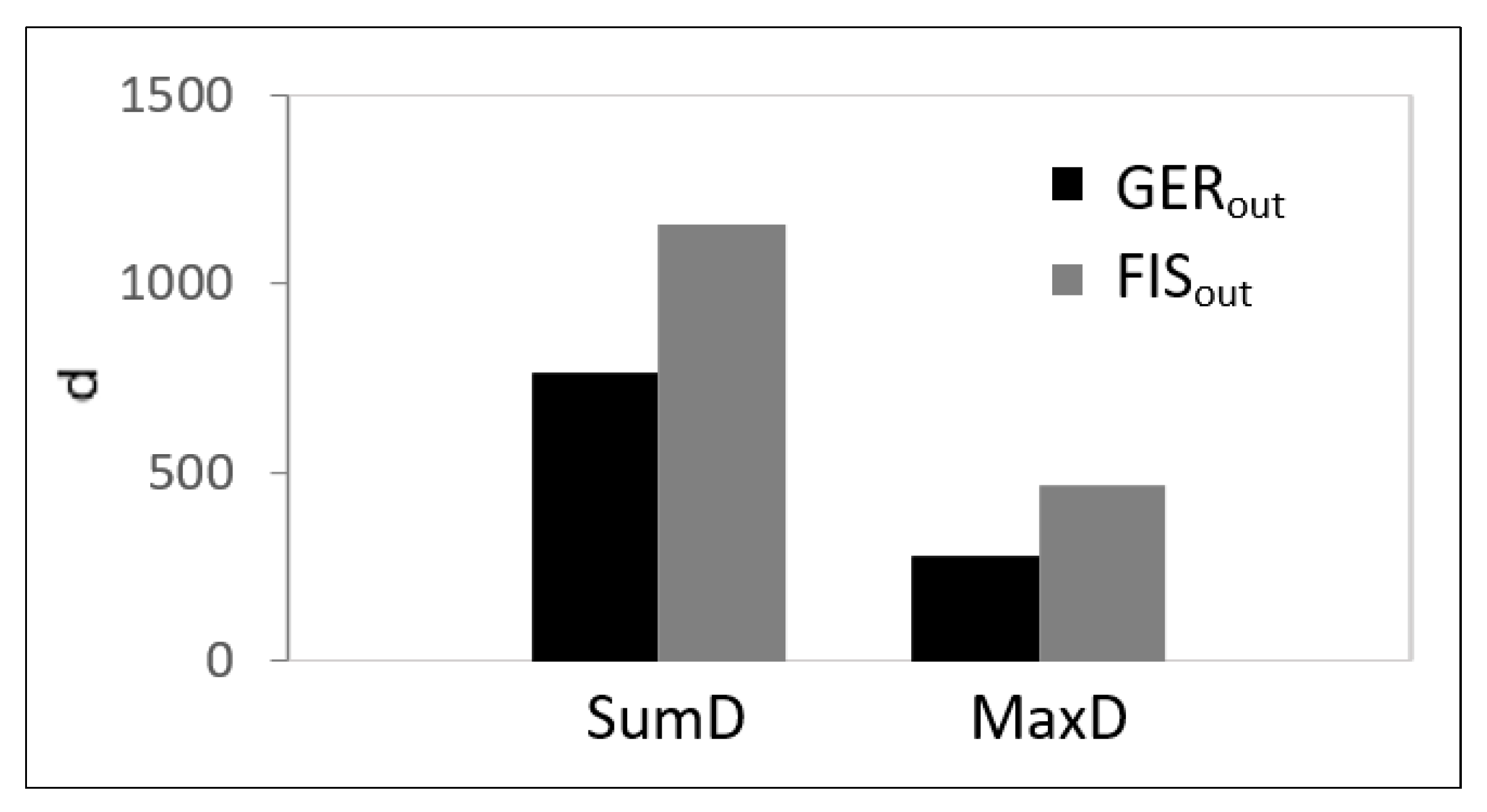
The total sums of characteristic values SumD and MaxD were found to be close to double as high in FIS_out compared to GER_out for the entire study period (Figure 11). On the other hand, GER_out was characterized by significantly trending increases in low flow occurrences and duration already for the lowest threshold (MAM). In FIS_out, SumD increased significantly at the 95% level solely for thresholds MAM7 and MAM30. The characteristic value MaxD was shown to increase only for the monthly threshold (MAM30). Resultantly, FIS_out experienced a high total number of low flow events throughout the study period, while in GER_out, the frequency and duration of low flow events per year increased significantly throughout the study period from 1980 to 2018.

An analysis of the change layers of the CORINE Land Cover (CLC) data sets did not reveal significant changes in land-use. Consequently, urban expansion or diversification of land-use may be ruled out as the reason for these depicted trends, leaving meteorological factors as the main impacting variables. Therefore, it is very likely that the significant increases in characteristic values SumD and MaxD in GER_out are linked to increasing T and decreasing P values. Additionally, PET rose at a higher rate in GER compared to FIS, very probably resulting in more low flow days per year [77].

The findings suggest that low flow in GER_out shows a higher sensitivity to climate-induced variability and has a greater long-term sensitivity towards droughts than in FIS_out. The ratio of MAM and $\overline{Q}$ in GER_out was shown to be lower than in FIS_out: while MAM/$\overline{Q}$ equals 0.25 in GER_out, the ratio equals 0.28 in FIS_out. In addition, the BFI in FIS_out was slightly higher than that in GER_out, at 0.45 and 0.44, respectively, with the actual BFI in GER_out probably being even lower, as the additional discharge in GER_out through wastewater treatment plants was not taken into account. Both the MAM/$\overline{Q}$ and the BFI indicate a higher sensitivity of GER_out towards hydrological extremes, such as droughts. However, these indices should be treated with care, as they were determined for a main catchment and its upstream subcatchment. Nevertheless, higher correlations between low flow indices and drought indices were also determined for GER_out. Subsequently, there seems to be a higher likelihood for drought-induced flows in GER_out compared to FIS_out.

The results suggest a longer duration of low flow events as well as a higher frequency of low flow in FIS_out from the catchment’s characteristics described in Section 2. While FIS is located in the crystalline Odenwald, the prevailing environments in GER are the Reinheimer Hügelland and the lower Main plain. While the elevations in the south measure up to 600 m.a.s.l., the lowest point of GER lies at about 100 m.a.s.l. Even though the altitude causes higher overall P, the steep slopes and the low usable field capacity of the soils prevailing in FIS lead to a high proportion of direct runoff while suggesting low buffering reserves of GW or intermediate storage [37]. Stoelzle et al. [20] found that hydrogeology has a decisive influence on how sensitive a catchment is towards short and long dry periods in Germany. It was shown that porous, complex aquifers have an increased long-term sensitivity towards droughts. This is in accordance with the findings in this paper. On the one hand FIS, which does not encompass any noticeable GW resources, showed high frequencies of low flow. On the other hand, GER, in which extended, porous aquifers are located, experienced low flow less frequently while showing a greater sensitivity towards the trends of changing climate variables. Staudinger et al. [78] state that catchments at lower elevations and low slopes, such as GER, are more sensitive towards meteorological droughts than catchments at higher elevations with steeper slopes, such as FIS, further supporting the findings of this study. In addition, the higher drainage density in the subcatchment suggests a lower permeability of the subsoil and less deep seepage. The domination of unconsolidated rock in the northern part of the catchment hint to overall better infiltration rates and storage capacities. Moreover, the smaller catchment size of FIS and the lower discharges make the stream more susceptible to dry and hot periods. While $\overline{Q}$ measured 0.34 m³/s in FIS_out for the entire observation period of 39 years, the average flow rate in GER_out measured 3.08 m³/s. While the Gersprenz is a small river, the Fischbach belongs to the category of streams. At the same evaporation rate, the losses in the Fischbach are expected to be higher than in the Gersprenz. In addition, the actual Evapotranspiration (ET) in the catchment may impact the catchments’ sensitivity towards droughts and low flows. The German Federal Institute of Hydrology (BfG) [79] estimated the average annual sums of actual ET for certain land-use types in Germany based on a method developed by Glugla et al. [80]. It was shown that the actual ET in forests was up to nearly 27% higher than in agricultural land-use types depending on the soil conditions and tree types. The prevailing land-use type in the subcatchment FIS is forests, while the prevailing land-use type in GER is agriculture. The PET determined with the Hargreaves equation was higher in GER than in FIS. However, the Hargreaves equation is based on the assumption of endless water availability and does not take into consideration land-use. Therefore, it is very likely that the actual ET is higher in the subcatchment, in which more than half of the area is covered in forests. Consequently, the impact of actual ET rates should also not be neglected. Finally, the evidence from this study suggests that FIS_out seems to be more prone to seasonal, short-term low-flow events, which do not necessarily inaugurate a meteorological drought [6], while low flow in GER_out is sensitive towards long-term changes of climatological variables, reflecting the trends of increasing magnitudes of drought events depicted for the study period.

In agreement with Smakhtin [6], the international glossary of hydrology [4] defines low flow as the “flow of water in a stream during prolonged dry weather”. This definition is adapted widely [81] and suggests an inherent relation between low flow and drought. The results of this study, however, emphasize that even small-scale system processes will influence low flow behavior. Therefore, extreme caution must be taken when analyzing the effects of droughts and trending climate variables on hydrological processes or when modeling low flow. This study showed that low flow is highly sensitive towards regional circumstances and catchment characteristics. In addition, the results emphasize the importance of antecedent conditions when identifying major low flow periods. The drought indicators SPI24 and SPEI24, which take into account climatic conditions of the 24 antecedent months, were most accurate in identifying years with extreme low flow behavior. This is in accordance with the study of Rolls et al. [1], which determined antecedent conditions as one of six ecologically relevant hydrological attributes of low flow. Generally, the superposition of influencing factors leads to a complex chain of effects. Nevertheless, the results of this study allow the conclusion that catchment characteristics and climatological variability and trends weigh differently in their impacts on low flow in different catchments. As a result, a climatic dry phase or drought does not necessarily result in low flow. Catchment characteristics significantly determine the sensitivity of the low flow behavior with respect to climate change.

5. Conclusions

This study showed that there has been a strong tendency towards drier and hotter years in the low mountain range basin of the river Gersprenz in the period of 1980 to 2018. This result is in coherence with the worldwide trend of global warming. Concurrently, the region was shown to experience droughts of increasing magnitudes throughout the study period. In addition, a general trend towards extreme low flows was proven for the study area. Thus, the results portray declining water availability for the Gersprenz and the Fischbach catchments. However, the catchments encompassed different trends and low-flow sensitivities. The evidence from this study suggests that the effects of drought on low flow depend on the catchment’s characteristics and the antecedent climate conditions.

In general, it was shown that a catchment’s sensitivity towards low flow is highly dependent on the site’s morphology, hydrogeology, prevailing land-use types, as well as catchment and stream size. Catchments comprising characteristics that are likely to evoke low flow (e.g., low water storage capacities, low seepage, steep slopes, low drainage densities, etc.) are probably more likely to experience short-term, seasonal low flow events. In contrast, catchments incorporating characteristics that are more robust towards fluctuations of water availability (e.g., high water storage capacities, high seepage, moderate terrain, high drainage densities, etc.) will show long-term sensitivities towards meteorological trends. As a consequence, it can be inferred that alteration and shaping of watershed properties can influence the low-flow sensitivity of the watershed. Taken together, this study emphasizes the importance of small-scale effects when dealing with low flow events, showing that even subcatchment characteristics will determine whether a low flow event is drought-induced. Despite the interaction of influencing factors complicating the determination of each individual factor’s role, this study can be seen as a further step in enhancing the understanding of low flow processes in river catchments.

References

- Rolls, R.J.; Leigh, C.; Sheldon, F. Mechanistic effects of low-flow hydrology on riverine ecosystems: Ecological principles and consequences of alteration. Freshw. Sci. 2012, 31, 1163–1186. [Google Scholar] [CrossRef] [Green Version]
- Burn, D.H.; Buttle, J.M.; Caissie, D.; MacCulloch, G.; Spence, C.; Stahl, K. The Processes, Patterns and Impacts of Low Flows Across Canada. Can. Water Resour. J. 2008, 33, 107–124. [Google Scholar] [CrossRef] [Green Version]
- Van Loon, A.F. Hydrological Drought Explained. WIREs Water 2015, 2, 359–392. [Google Scholar] [CrossRef]
- WMO: World Meteorological Organisation. International Glossary of Hydrology; WMO: Geneva, Switzerland, 1974. [Google Scholar]
- Vogt, J.; Somma, F. Drought and Drought Mitigation in Europe. In Advances in Natural and Technological Hazards Research; Springer: Dordrecht, The Netherlands, 2000. [Google Scholar] [CrossRef]
- Smakhtin, V.U. Low flow hydrology: A review. J. Hydrol. 2001, 240, 147–186. [Google Scholar] [CrossRef]
- Van Lanen, H.A.; Wanders, N.; Tallaksen, L.M.; Van Loon, A.F. Hydrological drought across the world: Impact of climate and physical catchment structure. Hydrol. Earth Syst. Sci. 2013, 17, 1715–1732. [Google Scholar] [CrossRef] [Green Version]
- UNFCCC. United Nations Framework Convention on Climate Change: Handbook; Climate Change Secretariat: Bonn, Germany, 2006. [Google Scholar]
- KLIWA (Klimaveränderung und Wasserwirtschaft). Niedrigwasser in Süddeutschland. Analysen, Szenarien und Handlungsempfehlungen, KLIWA-Berichte Heft 23; Deutscher Wetter Dienst (DWD), Landesanstalt für Umwelt Baden-Württemberg (LUBW), Bayerisches Landesamt für Umwelt (BLfU), Landesamt für Umwelt Rheinland-Pfalz (LfU); Arbeitskreis KLIWA: Offenbach, Germany; Karlsruhe, Germany; Hof, Germany; Mainz, Germany, 2018. [Google Scholar]
- HLNUG: Hessisches Landesamt für Naturschutz, Umwelt und Geologie. Klimawandel in Hessen: Beobachteter Klimawandel; HLNUG: Wiesbaden, Germany, 2018. [Google Scholar]
- Mühr, B.; Kubisch, S.; Marx, A.; Stötzer, J.; Wisotzky, C.; Latt, C.; Siegmann, F.; Glattfelder, M.; Mohr, S.; Kunz, M. Dürre & Hitzewelle Sommer 2018; Center for Disaster Management and Risk Reduction Technology (Karlsruhe Institute of Technology): Karlsruhe, Germany, 2018. [Google Scholar]
- Marx, A. UFZ: Helmholtz Zentrum für Umweltforschung. Dürremonitor Deutschland. Available online: www.ufz.de/index.php?de=37937 (accessed on 20 December 2020).
- University of Freiburg. Drought Projects. Available online: www.drought.uni-freiburg.de (accessed on 20 December 2020).
- Teuling, A.J.; Van Loon, A.F.; Seneviratne, S.I.; Lehner, I.; Aubinet, M.; Heinesch, B.; Bernhofer, C.; Grünwald, T.; Prasse, H.; Spank, U. Evapotranspiration amplifies European summer drought. Geophys. Res. Lett. 2013, 40, 2071–2075. [Google Scholar] [CrossRef]
- Kormos, P.R.; Luce, C.H.; Wenger, S.J.; Berghuijs, W.R. Trends and sensitivities of low streamflow extremes to discharge timing and magnitude in Pacific Northwest mountain streams. Water Resour. Res. 2016, 52, 4990–5007. [Google Scholar] [CrossRef] [Green Version]
- Jones, R.N.; Chiew, F.H.; Boughton, W.C.; Zhang, L. Estimating the sensitivity of mean annual runoff to climate change using selected hydrological models. Adv. Water Resour. 2006, 29, 1419–1429. [Google Scholar] [CrossRef] [Green Version]
- Safeeq, M.; Fares, A. Hydrologic response of a Hawaiian watershed to future climate change scenarios. Hydrol. Process. 2012, 26, 2745–2764. [Google Scholar] [CrossRef]
- Bowling, L.; Egan, S.; Holliday, J.; Honeyman, G. Did spatial and temporal variations in water quality influence cyanobacterial abundance, community composition and cell size in the Murray River, Australia during a drought-affected low-flow summer? Hydrobiologia 2016, 765, 359–377. [Google Scholar] [CrossRef]
- Haslinger, K.; Koffler, D.; Schöner, W.; Laaha, G. Exploring the link between meteorological drought and streamflow: Effects of climate-catchment interaction. Water Resour. Res. 2014, 50, 2468–2487. [Google Scholar] [CrossRef]
- Stoelzle, M.; Stahl, K.; Morhard, A.; Weiler, M. Streamflow sensitivity to drought scenarios in catchments with different geology. Geophys. Res. Lett. 2014, 41, 6174–6183. [Google Scholar] [CrossRef]
- WMO: World Meteorological Organisation. Manual on Low-Flow Estimation and Prediction—Operational Hydrology Report No. 50; WMO: Geneva, Switzerland, 2008. [Google Scholar]
- Maniak, U. Hydrologie und Wasserwirtschaft: Eine Einführung für Ingenieure, 7th ed.; Springer: Berlin, Germany, 2016. [Google Scholar]
- Engeland, K.; Hisdal, H.; Beldring, S. Predicting low flows in ungauged catchments. In Climate Variability and Change: Hydrological Impacts, Proceedings of the Fifth FRIEND World Conference, Havana, Cuba, 27 November–1 December 2006; Demuth, S., Gustard, A., Planos, E., Scatena, F., Servat, E., Eds.; IAHS Press: Wallingford, UK, 2006; Volume 308, pp. 163–168. [Google Scholar]
- Eng, K.; Milly, P.C.D. Relating low-flow characteristics to the base flow recession time constant at partial record stream gauges. Water Resour. Res. 2007, 43. [Google Scholar] [CrossRef] [Green Version]
- Tokarczyk, T.; Jakubowski, W. Temporal and spatial variability of drought in mountain catchments of the Nysa Klodzka basin. In Climate Variability and Change: Hydrological Impacts, Proceedings of the Fifth FRIEND World Conference, Havana, Cuba, 27 November–1 December 2006; Demuth, S., Gustard, A., Planos, E., Scatena, F., Servat, E., Eds.; IAHS Press: Wallingford, UK, 2006; Volume 308, pp. 139–144. [Google Scholar]
- Peters, E.; Bier, G.; van Lanen, H.; Torfs, P. Propagation and spatial distribution of drought in a groundwater catchment. J. Hydrol. 2006, 321, 257–275. [Google Scholar] [CrossRef]
- Trambauer, P.; Werner, M.; Winsemius, H.C.; Maskey, S.; Dutra, E.; Uhlenbrook, S. Hydrological drought forecasting and skill assessment for the Limpopo River basin, southern Africa. Hydrol. Earth Syst. Sci. 2015, 19, 1695–1711. [Google Scholar] [CrossRef] [Green Version]
- Menzel, L. Hydrologische Extreme: Dürren. In Hydrologie; Fohrer, N., Bormann, H., Miegel, K., Casper, M., Bronstert, A., Schumann, A., Weiler, M., Eds.; Haupt Verlag: Bern, Switzerland, 2016; pp. 223–229. [Google Scholar]
- HLNUG: Hessisches Landesamt für Naturschutz, Umwelt und Geologie. Niedrigwasser und Trockenheit 2018; HLNUG: Wiesbaden, Germany, 2018.
- Douglas, E.; Vogel, R.; Kroll, C. Trends in floods and low flows in the United States: Impact of spatial correlation. J. Hydrol. 2000, 240, 90–105. [Google Scholar] [CrossRef]
- Schmalz, B.; Kruse, M. Impact of Land Use on Stream Water Quality in the German Low Mountain Range Basin Gersprenz. Landsc. Online 2019, 72, 1–17. [Google Scholar] [CrossRef] [Green Version]
- EC. European Water Framework Directive. In Richtlinie 2000/60/EG des Europäischen Parlaments und des Rates vom 23. Oktober 2000 zur Schaffung eines Ordnungsrahmens für Maßnahmen der Gemeinschaft im Bereich der Wasserpolitik; European Parliament: Brussels, Belgium, 2000. [Google Scholar]
- HLNUG: Hessisches Landesamt für Naturschutz, Umwelt und Geologie. Discharge Data of the Gauges Harreshausen (ID: 24762653) and Groß Bieberau 2 (ID: 24761005); HLNUG: Wiesbaden, Germany, 2019.
- HVBG: Hessian Agency for Land Management and Geoinformation. ATKIS ©. Amtliches Topographisch-Kartographisches Informations System [Authorative Topographic-Cartographic Information System]; HVBG: Wiesbaden, Germany, 2017. [Google Scholar]
- DWD: Deutscher Wetterdienst. CDC—Climate Data Center. Observations Germany. Available online: https://cdc.dwd.de/portal/ (accessed on 26 March 2020).
- Horton, R.E. Erosional Development Of Streams And Their Drainage Basins; Hydrophysical Approach To Quantitative Morphology. Geol. Soc. Am. Bull. 1945, 56, 275–370. [Google Scholar] [CrossRef] [Green Version]
- HLNUG: Hessisches Landesamt für Naturschutz, Umwelt und Geologie. Hydrogeologie von Hessen–Odenwald und Sprendlinger Horst. (Grundwasser in Hessen, Heft 2); HLNUG: Wiesbaden, Germany, 2017.
- BfG: Bundesanstalt für Gewässerkunde. Hydrologischer Atlas Deutschland. Available online: https://geoportal.bafg.de/mapapps/resources/apps/HAD/index.html?lang=de (accessed on 5 November 2020).
- BGR: Bundesanstalt für Geowissenschaften und Rohstoffe. Hydrogeologische Karten für den Hydrologischen Atlas von Deutschland. Mittlere jährliche Grundwasserneubildung (GWN1000). Available online: https://www.bgr.bund.de/DE/Themen/Wasser/Produkte/produkte_node.html (accessed on 20 December 2020).
- Neumann, J. Flächendifferenzierte Grundwasserneubildung von Deutschland—Entwicklung und Anwendung des makroskaligen Verfahrens HAD-GWNeu. Ph.D. Thesis, Martin-Luther-Universität Halle-Wittenberg, Halle/Saale, Germany, 2004. [Google Scholar]
- LfU: Bayrisches Landesamt für Umwelt. Grundwasserneubildung. Available online: https://www.lfu.bayern.de/wasser/grundwasserneubildung/index.htm (accessed on 30 November 2020).
- Bloomfield, J.P.; Allen, D.J.; Griffiths, K.J. Examining geological controls on baseflow index (BFI) using regression analysis: An illustration from the Thames Basin, UK. J. Hydrol. 2009, 373, 164–176. [Google Scholar] [CrossRef] [Green Version]
- Kissel, M.; Schmalz, B. Comparison of Baseflow Separation Methods in the German Low Mountain Range. Water 2020, 12, 1740. [Google Scholar] [CrossRef]
- Kille, K. Das Verfahren MoMNQ, ein Beitrag zur Berechnung der mittleren langjährigen Grundwasserneubildung mit Hilfe der monatlichen Niedrigwasserabflüsse. Z. Dt. Geol. Ges. Sonderh. Hydrogeol. 1970, 89–95. [Google Scholar]
- HLNUG: Hessisches Landesamt für Naturschutz, Umwelt und Geologie. WRRL-Viewer. Das Fachinformationssystem des Landes Hessen Rund um das Thema EG-Wasserrahmenrichtlinie (WRRL). Available online: http://wrrl.hessen.de/mapapps/resources/apps/wrrl/index.html?lang=de (accessed on 12 November 2020).
- Gorte, B.G.H. Land-Use and Catchment Characteristics. In Remote Sensing in Hydrology and Water Management; Schultz, G.A., Engman, E.T., Eds.; Springer: Berlin/Heidelberg, Germany, 2000; pp. 133–156. [Google Scholar] [CrossRef]
- EEA: European Environment Agency. Copernicus Land Monitoring Service—Corine Land Cover. Available online: https://www.eea.europa.eu/data-and-maps/data/copernicus-land-monitoring-service-corine (accessed on 20 December 2020).
- Jörs, R. Gersprenz Findet Zurück zur Natur. In ECHO; Available online: https://www.echo-online.de/lokales/darmstadt-dieburg/eppertshausen/gersprenz-findet-zuruck-zur-natur_17544647 (accessed on 20 December 2020).
- LOKALES: Odenwaldkreis. Wasserentnahme aus Gersprenz Verboten. Available online: https://www.echo-online.de/lokales/odenwaldkreis/odenwaldkreis/wasserentnahme-aus-gersprenz-verboten_18907046 (accessed on 20 December 2020).
- HVBG: Hessian Agency for Land Management and Geoinformation. Digital Elevation Model (ATKIS® DGM)—1 m Resolution; HVBG: Wiesbaden, Germany, 2017. [Google Scholar]
- Li, J.; Chen, Y.D.; Gan, T.Y.; Lau, N.C. Elevated increases in human-perceived temperature under climate warming. Nat. Clim. Change 2018, 8, 43–47. [Google Scholar] [CrossRef]
- Tesfaye, S.; Taye, G.; Birhane, E.; van der Zee, S.E. Observed and model simulated twenty-first century hydro-climatic change of Northern Ethiopia. J. Hydrol. Reg. Stud. 2019, 22, 100595. [Google Scholar] [CrossRef]
- Del Toro-Guerrero, F.J.; Kretzschmar, T. Precipitation-temperature variability and drought episodes in northwest Baja California, México. J. Hydrol. Reg. Stud. 2020, 27, 100653. [Google Scholar] [CrossRef]
- DWD: Deutscher Wetterdienst. Dokumentation: Standardized Precipitation Index SPI; DWD: Offenbach, Germany, 2015.
- McKee, T.B.; Doesken, N.J.; Kleist, J. The relationship of drought frequency and duration to time scale. In Proceedings of the Eighth Conference on Applied Climatology, Anaheim, CA, USA, 17–22 January 1993; pp. 179–184. [Google Scholar]
- WMO: World Meteorological Organization. Standardized Precipitation Index User Guide; WMO: Geneva, Switzerland, 2012. [Google Scholar]
- Povoa, L.V.; Nery, J.T. Precipitation Intensity, Concentration and Anomaly Analysis. Available online: https://cran.r-project.org/web/packages/precintcon/precintcon.pdf (accessed on 20 December 2020).
- Wu, F.F.; Yang, X.H.; Shen, Z.Y. A three-stage hybrid model for regionalization, trends and sensitivity analyses of temperature anomalies in China from 1966 to 2015. Atmos. Res. 2018, 205, 80–92. [Google Scholar] [CrossRef]
- Vicente-Serrano, S.M.; Beguería, S.; López-Moreno, J.I. A Multiscalar Drought Index Sensitive to Global Warming: The Standardized Precipitation Evapotranspiration Index. J. Clim. 2010, 23, 1696–1718. [Google Scholar] [CrossRef] [Green Version]
- Hargreaves, G.H.; Samani, Z.A. Reference Crop Evapotranspiration from Temperature. Appl. Eng. Agric. 1985, 1, 96–99. [Google Scholar] [CrossRef]
- Čadro, S.; Uzunović, M. How to Use: Package ‘SPEI’ For Basic Calculations; 2013; Available online: https://cran.r-project.org/web/packages/SPEI/SPEI.pdf (accessed on 21 September 2020). [CrossRef]
- Bindi, M.; Brandani, G.; Dessì, A. Impact of Climate Change on Agricultural and Natural Ecosystems; Firenze University Press: Florence, Italy, 2009. [Google Scholar]
- DIN4049: Deutsches Institut für Normung e.V. DIN 4049 Teil 3: Begriffe zur Quantitativen Hydrologie; Deutsches Institut für Normung e.V.: Berlin, Germany, 1994. [Google Scholar]
- Eslamian, S.; Eslamian, F.A. Handbook of Drought and Water Scarcity: Environmental Impacts and Analysis of Drought and Water Scarcity; CRC Press: Boca Raton, FL, USA, 2017; Volume 1. [Google Scholar]
- Svensson, C.; Kundzewicz, W.Z.; Maurer, T. Trend detection in river flow series: 2. Flood and low-flow index series. Hydrol. Sci. J. 2005, 50, 824. [Google Scholar] [CrossRef] [Green Version]
- Kay, A.L.; Bell, V.A.; Guillod, B.P.; Jones, R.G.; Rudd, A.C. National-scale analysis of low flow frequency: Historical trends and potential future changes. Clim. Chang. 2018, 147, 585–599. [Google Scholar] [CrossRef] [Green Version]
- LfU: Bayrisches Landesamt für Umwelt. Kenn-und Schwellenwerte für Niedrigwasser. Begriffserläuterungen und Methodik für Auswertungen am LfU. Available online: https://www.lfu.bayern.de/wasser/klima_wandel/auswirkungen/niedrigwasserabfluesse/doc/niedrigwasserkennwerte.pdf (accessed on 5 March 2020).
- Staudinger, M.; Stoelzle, M.; Seeger, S.; Seibert, J.; Weiler, M.; Stahl, K. Catchment water storage variation with elevation. Hydrol. Process. 2017, 31, 2000–2015. [Google Scholar] [CrossRef]
- DVWK: Deutsche Vereinigung für Wasserwirtschaft, Abwasser und Abfall e.V. Niedrigwasseranalyse; Teil 1: Statistische Untersuchung des Niedrigwasser-Abflusses; Parey: Hamburg, Germany, 1983. [Google Scholar]
- IKSR: Internationale Kommission zum Schutz des Rheins. Bestandsaufnahme zu den Niedrigwasserverhältnissen am Rhein. Bericht Nr. 248; IKSR: Koblenz, Germany, 2018. [Google Scholar]
- Wang, K.; Liu, X.; Tian, W.; Li, Y.; Liang, K.; Liu, C.; Li, Y.; Yang, X. Pan coefficient sensitivity to environment variables across China. J. Hydrol. 2019, 572, 582–591. [Google Scholar] [CrossRef]
- NOAA: National Oceanic and Atmospheric Administration—National Centers for Environmental Information. State of the Climate: Global Climate Report for Annual 2019; NOAA: Washington, DC, USA, 2019.
- IPCC: Intergovernmental Panel on Climate Change. Climate Change 2014: Synthesis Report. Contribution of Working Groups I, II and III to the Fifth Assessment Report of the Intergovernmental Panel on Climate Change; IPCC: Geneva, Switzerland, 2014. [Google Scholar]
- Booij, M.J.; Huisjes, M.; Hoekstra, A.Y. Uncertainty in climate change impacts on low flows. In Climate variability and Change: Hydrological Impacts, Proceedings of the Fifth FRIEND World Conference, Havana, Cuba, 27 November–1 December 2006; Demuth, S., Gustard, A., Planos, E., Scatena, F., Servat, E., Eds.; IAHS Press: Wallingford, UK, 2006; Volume 308, pp. 401–406. [Google Scholar]
- Labudová, L.; Labuda, M.; Takáč, J. Comparison of SPI and SPEI applicability for drought impact assessment on crop production in the Danubian Lowland and the East Slovakian Lowland. Theor. Appl. Climatol. 2017, 128, 491–506. [Google Scholar] [CrossRef]
- Belz, J.; Brahmer, G.; Buiteveld, H.; Engel, H.; Grabher, R.; Hodel, H.; van Vuuren, W. Das Abflussregime des Rheins und Seiner Nebenflüsse im 20. Jahrhundert—Analyse, Veränderungen, Trends; KHR-Bericht Nr. I-22; International Commission for the Hydrology of the Rhine basin (CHR): Koblenz, Germany; Lelystad, The Netherlands, 2007. [Google Scholar]
- Roderick, M.L.; Sun, F.; Lim, W.H.; Farquhar, G.D. A general framework for understanding the response of the water cycle to global warming over land and ocean. Hydrol. Earth Syst. Sci. 2014, 18, 1575–1589. [Google Scholar] [CrossRef] [Green Version]
- Staudinger, M.; Weiler, M.; Seibert, J. Quantifying sensitivity to droughts: An experimental modeling approach. Hydrol. Earth Syst. Sci. 2015, 19, 1371–1384. [Google Scholar] [CrossRef] [Green Version]
- BfG: Bundesanstalt für Gewässerkunde. Mittlere Jährliche Verdunstungshöhe. Available online: https://geoportal.bafg.de/dokumente/had/Verdunstungshoehe.pdf (accessed on 30 November 2020).
- Glugla, G.; Jankiewicz, P.; Rachimow, C.; Lojek, K.; Richter, K.; Fürtig, G.; Krahe, P. BAGLUVA–Wasserhaushaltsverfahren zur Berechnung vieljähriger Mittelwerte der tatsächlichen Verdunstung und des Gesamtabflusses. In BfG-Bericht; Bundesanstalt für Gewässerkunde: Koblenz, Germany, 2003; Volume 1342, p. 102. [Google Scholar]
- EPA: United States Environmental Protection Agency. Definition and Characteristics of Low Flows. Available online: https://www.epa.gov/ceam/definition-and-characteristics-low (accessed on 21 September 2020).
Figure 1.
Field laboratory located in the federal state of Hesse in Germany.
Figure 2.
Drainage density in the Gersprenz (GER) and Fischbach (FIS) in km/km2 (data source: BfG [38]).
Figure 3.
Groundwater resources in the GER and FIS (data source: BfG [38]).
Figure 4.
Ranked monthly flow minima according to Kille [44] and mean baseflow value in GERout and FISout. The green dots are manually selected interpolation points for the fitted red line. Based on daily flow data from the HLNUG [33].
Figure 5.
Locations of measurement stations (data source: HVBG (50)).
Figure 6.
Deviations of annual mean temperatures and annual precipitation to long-term averages in GER (top) and FIS (bottom): the years 2018, 2015, 2011, and 1991 were identified as exceptionally dry.
Figure 7.
Drought indices SPI and SPEI for 3-, 6-, 12-, and 24 months in GER.
Figure 8.
Drought indices SPI and SPEI for 3-, 6-, 12-, and 24 months in FIS.
Figure 9.
AMIN, AMIN7, and AMIN30 time series with linear trends given for the AMIN30 data in GERout and FISout.
Figure 10.
Scatterplot presenting SumD and MaxD values for the threshold MAM7 for each year of the study period 1980–2018: the size of each circle indicates the number of MAM7 days necessary to balance out the deficit of each year (scheme inspired by KLIWA [9]).
Figure 11.
Total SumD and MaxD values for the MAM threshold in GERout and FISout (1980–2018).