Assessment of Streamflow Simulation for a Tropical Forested Catchment Using Dynamic TOPMODEL—Dynamic fluxEs and ConnectIvity for Predictions of HydRology (DECIPHeR) Framework and Generalized Likelihood Uncertainty Estimation (GLUE)

Abstract

Rainfall runoff modeling has been a subject of interest for decades due to a need to understand a catchment system for management, for example regarding extreme event occurrences such as flooding. Tropical catchments are particularly prone to the hazards of extreme precipitation and the internal drivers of change in the system, such as deforestation and land use change. A model framework of dynamic TOPMODEL, DECIPHeR v1—considering the flexibility, modularity, and portability—and Generalized Likelihood Uncertainty Estimation (GLUE) method are both used in this study. They reveal model performance for the streamflow simulation in a tropical catchment, i.e., the Kelantan River in Malaysia, that is prone to flooding and experiences high rates of land use change. Thirty-two years’ continuous simulation at a daily time scale simulation along with uncertainty analysis resulted in a Nash Sutcliffe Efficiency (NSE) score of 0.42 from the highest ranked parameter set, while 25.35% of the measurement falls within the uncertainty boundary based on a behavioral threshold NSE 0.3. The performance and behavior of the model in the continuous simulation suggests a limited ability of the model to represent the system, particularly along the low flow regime. In contrast, the simulation of eight peak flow events achieves moderate to good fit, with the four peak flow events simulation returning an NSE > 0.5. Nonetheless, the parameter scatter plot from both the continuous simulation and analyses of peak flow events indicate unidentifiability of all model parameters. This may be attributable to the catchment modeling scale. The results demand further investigation regarding the heterogeneity of parameters and calibration at multiple scales.

1. Introduction

A work of hydrological modeling research is an interactive learning of data and the knowledge—i.e., process understanding, theory, and a model structure [1]. Modeling has greatly improved by increases in computing power and sophistication within the last 20 years, not only in reference to the computing capability but also the availability of remote sensing data [2] that supplement field measurement data. These developments result in an evolution of hydrological models into more sophisticated forms, particularly in terms of model complexity and spatial scale such as in a physically based distributed model [3,4]. However, the higher the complexity of a model structure may be, the more data is required and the greater number of parameters needed to be calibrated and validated [2]. For a large catchment with data scarcity issues [5,6], a model with less structural complexity, for example that in the form of a distributed conceptual model, may be a better alternative.

A conceptual model is built based on a perception of a complex system that is described into mathematical equations and coded for a computer simulation [7]. The physical process is simplified into components of storage and transfer between them that are controlled by the water balance equation [5,6]. Conceptual rainfall runoff models such as HBV, PDM, and TOPMODEL are commonly used due to their simplicity and practicality yet at the same time having a sound scientific basis [8,9]. Nevertheless, all models have their own limitations and, furthermore, they may not produce comparable results. TOPMODEL, for example, was developed for a hillslope and found to underperform in simulations of groundwater levels and the distribution of saturated areas [10]. Nevertheless, further improvements to the original model were made by adding a groundwater term as a local storage deficit based on a field survey produced good model performance [11]. Later, a dynamic version of the model introduced the kinematic wave solution aiming to remove the rigid assumption required for the original version that the water table is defined as a succession of steady states, neglecting the groundwater temporal response [12]. TOPMODEL, intentionally introduced as a concept [7], was made publicly available by the recent works of the Dynamic TOPMODEL (DynaTOPMODEL) framework development in R [13] and Dynamic fluxEs and ConnectIvity for Predictions of Hydrology (DECIPHeR v1) coded in FORTRAN [14].

Both frameworks offer the advantages of accessibility, modularity, and portability [15]. These allow the needed interactive learning previously mentioned for an individual catchment. This is achieved by taking into account the issue of the uniqueness of a catchment [7], data availability, and model structure adaptation to a certain application in practice [9]. Just released in 2018, DECIPHeR version 1, which is used in this study, is a flexible model framework available as an open source via github. The distributed concept in the model is explained ranging from the Hydrological Response Unit (HRU) definition being lumped—whereby a single HRU covers the entire catchment—to fully distributed where an HRU is assigned for every grid cell [14]. DECIPHeR, which was on purpose developed for a wide range of spatial and temporal scales [14], allows simulation on multiple catchments and the experimentation of new concepts to capture the complexity and the heterogeneity in a catchment system through additional model structure and related parameters [14]. A single structure is introduced in the model with a built-in option of Monte Carlo sampling to generate the random parameter sets distribution used for uncertainty analysis.

The Generalized Likelihood Uncertainty Estimation (GLUE) methodology of the uncertainty analysis frameworks in hydrological modeling [16] can be used to analyze model parameter uncertainty and understand model behavior. There have been arguments that the method is subjective mainly for the threshold assumption [16,17] and suggestions to value the method as a weighted sensitivity analysis instead of a probabilistic method [18]. The threshold assumption is intended as a boundary of acceptability, where values above the threshold are considered to be behavioral [19] and are further used in the uncertainty analysis. The method where many sets of parameters provides acceptable simulation results—a concept known as equifinality [19,20]—is common [21,22] for assessing the model’s behavior toward the observed behavior of the system.

There have been few applications of the TOPMODEL based model such as DECIPHeR to a tropical forested catchment. The original TOPMODEL was reportedly used in a variety of small sized tropical catchments [23,24]. It has been also applied in Peninsular Malaysia, Malaysian Borneo and Thailand for short periods of observed data [25,26,27]. The model was mostly applied on small catchments [13,28,29], some are due to field measurement and used in the model analysis [11,26,27,30]. The implementation on a large scale catchment has also been attempted [31] with modification of block-wise [32], multiple catchment [14] and global scale applications [33].

The study area, Kelantan catchment (12,142 Km²) Peninsular Malaysia, is a large catchment with a tendency to experience extreme flooding [34] and significant land use change. Recent flood events were in 2014 and 2017 [35,36]. The highest water level recorded in the Kelantan catchment was in 2014, which highlights the important work of hydrological research [34]. A land use classification study for 20 years, from 1994 to 2014, revealed a 13.7% decrease in forest land and a 6.2% increase in oil palm plantations [37] in the catchment. These spurred many hydrological and modeling studies to be conducted in the area [38,39]. Some modeling studies on the Kelantan catchment adopted semidistributed approaches like HEC-HMS in modeling runoff using the Soil Conservation Service Curve Number (SCS-CN) method [39,40,41]. There have been studies that reported good model performance using the method [37,39]. Other methods such as the Integrated Flood Analysis System (IFAS) [38] have also been applied. However, the CN method, which imposes an empirical approach, has been developed based on humid rain-fed agricultural areas and is noted to performing poorly for a forested catchment [42]. Other model applications in the Kelantan catchment are either lumped conceptual models [43,44] where the performance varied with poor validation (R2 < 0.5), or based on machine learning approaches [45], where the performance is better (NSE > 0.9). Unlike in the lumped model where the processes were not made explicit, the machine learning is able to “learn” the surface-subsurface complexity from the data but is not spatially identified.

However, uncertainty analysis is a significant missing aspect of these existing works, which treated models as robust prediction tools rather than a means of improving system understanding. It is obvious that the entire process of modeling either the simplified or the complex assumption does inherit uncertainty due to data or/and a model assumption [16]. The common practice in a model calibration has been accepting a set of parameters based on performance measure values. On the other hand, in the uncertainty approach, the confidence interval is built based on the numbers of parameter sets considered to be behavioral toward the observed value of the system [19]. The range of parameters, instead of exact values, offers a wider scope of understanding the system.

The objective of this paper is to test the DECIPHeR model framework in a typical tropical forested catchment to assess the performance and the uncertainty of the model toward the system. The model is applied for the continuous time period from 1985 to 2016; an analysis on shorter segmented peak flow periods are also presented. The assumption of homogeneous parameters is used, neglecting the spatial complexity of the system. The model simulation is analyzed in terms of the uncertainty intervals to gain understanding on the differences between performances during different events and towards identifying the model parameters responsible for the deviations from the observations.

2. Materials and Methods

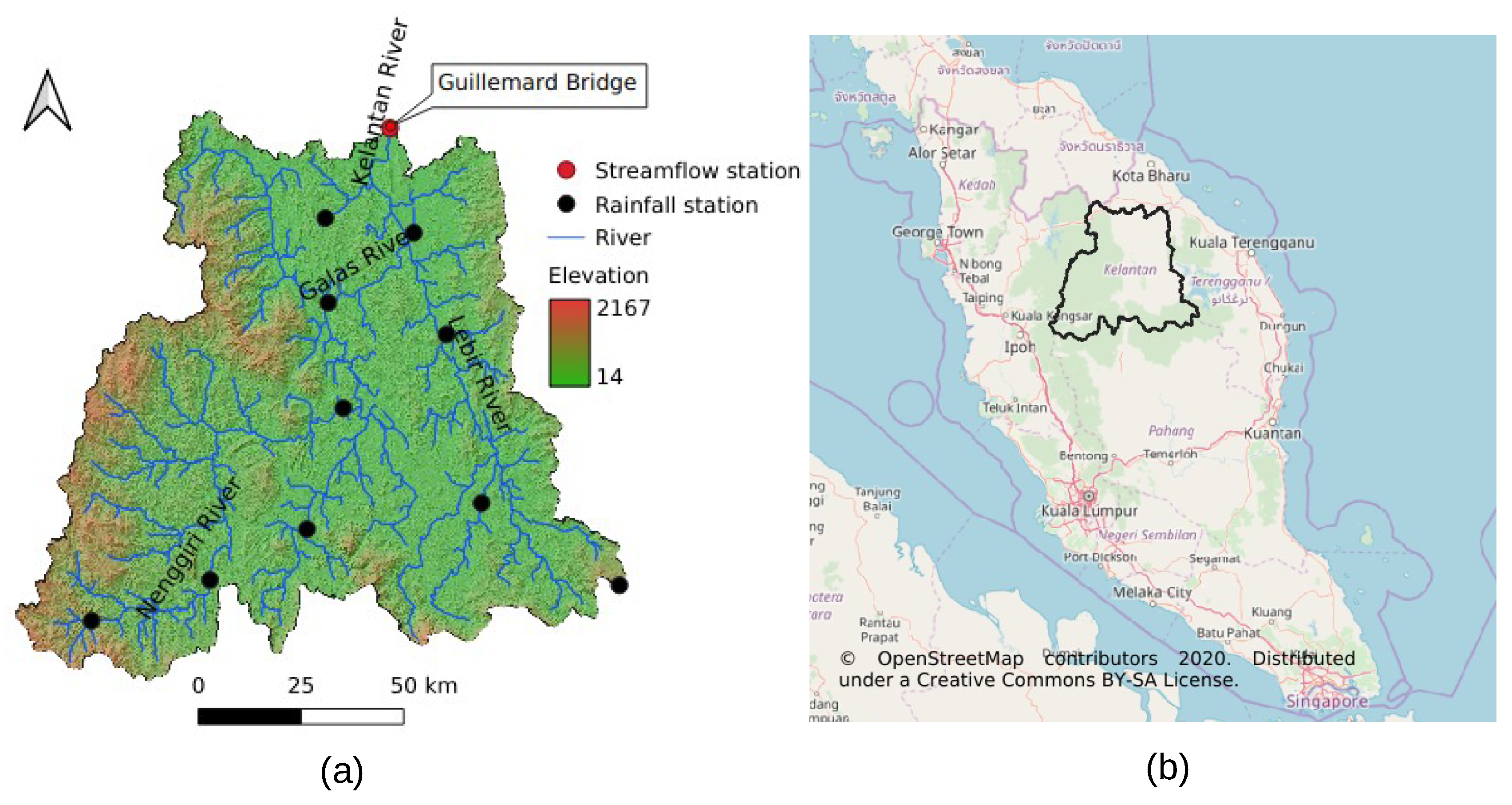
2.1. Study Area

The Kelantan catchment is located in the northern part of Malaysia Peninsular, geographically bounded between 4${}^{\circ }$30${}^{\prime }$ N to 6${}^{\circ }$15${}^{\prime }$ N latitude and 101${}^{\circ }$ E to 102${}^{\circ }$45${}^{\prime }$ E. The main tributaries are the Nenggiri, Galas, Lebir and Kelantan Rivers, Figure 1. The mean annual precipitation of the peninsula is around 2300 mm [46]. Considering the length of streamflow data availability, the catchment is delineated given the output at Station Sg. Kelantan at Guillemard Bridge. The delineated area is calculated using the Digital Terrain Analysis (DTA) in the DECIPHeR as 12,142 Km². The population of Kelantan based on 2015 data is 1.718 million [47] with approximately one third of the population living in the downstream area of the catchment [34], which is the most flood-prone.

2.2. Input Data

The main input data required by the model are: Digital Elevation Model (DEM), rainfall data, discharge data and evapotranspiration data. The DEM used is the Shuttle Radar Topography Mission (SRTM) 1 Arc-Second Global elevation data retrieved from https://earthexplorer.usgs.gov provided by the United State Geological Survey (USGS). The data set comes in tiles of 1 degree size, 30 m of spatial resolution and WGS84 Geographic (EPSG: 4326) [48]. The data set has been recognized by the hydrologic modeling community for its near-global coverage and high-resolution [49]. It is also reported that the quality of the SRTM data of the X-SAR band, after being validated with the reference DEM data set of two sites in Southern Germany, is sufficient for the TOPMODEL application on a medium scale catchment [49]. Hence, no further validation process was taken in this study.

The historical daily data of rainfall and discharge are acquired from The Department of Irrigation and Drainage (DID) of Malaysia. Ten rainfall gauge stations within the catchment and the streamflow station at the Guillemard Bridge of 32 years period from 1 January 1985–31 December 2016 are used for the model driving data. The gauges’ spatial distribution is shown in Figure 1. The gauged rainfall is converted to gridded rainfall after applying the Thiessen Polygon method for the gauges’ areal coverage. The polygon is aggregated into the grid size of the DEM, with every grid assigned to hold the value of the related gauges. The gauges were selected considering the least missing data record.

Global Land Evaporation Amsterdam Model (GLEAM) datasets, which provide different components of evapotranspiration separately based on satellite data [50,51], is also used in this study. A global validation was already applied to the provided data set using a large database from 2325 in situ sensors and 91 Eddy-covariance towers which returns correlation between 0.78 and 0.81 for evaporation fluxes [50]. The data retrieved is the potential evaporation in unit mm/day from GLEAM v3 which is stored in 3D array, on a 0.25${}^{\circ }$ × 0.25${}^{\circ }$ latitude-longitude grid and in a daily temporal resolution. The grid is also converted into the projection of the DEM and aggregated into the similar grid size. The data value is resampled into the new grid using bilinear interpolation.

2.3. The Concept and the Framework of the Rainfall Runoff Model

The original conceptual rainfall-runoff TOPMODEL has been known for the hydrological similarity points theory based on the topographic index $ln(atan\beta )$, assuming the saturated zone as a result of the successive steady state of the upslope area [7,52]. The dynamic version has been introduced by replacing the assumption of quasi steady state with the kinematic wave routing, while keeping the exponential transmissivity assumption, controlled by parameter $SZM$, and truncated by parameter $S_{max}$ [12,13,14].

The model, which was introduced as a concept rather than a tool [53], has not been publicly available until recently via the Dynamic TOPMODEL in R [13] and the DECIPHeR model framework which is coded in FORTRAN [14]. The DECIPHeR framework used in this study offers more advantages compared to the R version, which is applicable only for a single catchment. The framework was developed with the flexibility allowing users to explore a wider system from a single catchment up to multicatchments at a continental scale to modify the model structure by embedding a different conceptualization and to vary parameters recognizing a site specific issue by adding variability of spatial data layers such as land cover. The model is run in two steps, the DTA and Rainfall-Runoff Model. Using DEM, gauges’ coordinates, rainfall data grid, and the potential evapotranspiration data grid, the DTA is run to produce: (1) HRUs and the connectivity in the landscape, (2) river network and the routing properties, and (3) the extent and the simulated output location.

The assumption of the model is that the lateral fluxes in the saturated zone of an each elemental effective upslope contributing area a in the topographic index is numerically solved using the kinematic solution [12]. The flow is proportionally distributed between HRU and a river reach using a matrix, Equation (1), weighed by accumulated area and slope. Each HRU contains information of topographic information, inputs, the model structure, and the parameters set [14]. A wide range of parameters is used for the Monte Carlo sampling, as introduced in the DECIPHeR and presented in

Table 1. The dynamic TOPMODEL parameters range.

Parameter	Description	Lower Limit	Upper Limit
$SZM$ [m]	Form of exponential decline in conductivity	0.001	0.07
$ln\left(T_0\right)ln$[m${}^2$ h${}^{-1}$]	Effective lateral saturated transmissivity	−7	5
$S{r}_{max}$ [m]	Maximum root zone storage	0.005	0.15
$S{R}_{init}$ [m]	Initial root zone deficit	0	0.01
$T_d$ [m h${}^{-1}$]	Unsaturated zone time delay	0.1	40
$CHV$ [m h${}^{-1}$]	Channel routing velocity	250	4000
$S_{max}$ [m]	Maximum effective deficit of subsurface saturated zone	0.2	3

.

$$W=\left[\begin{array}{ccc}{w}_{11}& \cdots & w_{1n}\\ ⋮& \ddots & ⋮\\ w_{n1}& \cdots & w_{nn}\end{array}\right]$$

(1)

where ${\sum }_{i=1}^n{w}_{ij}=1$.

RR is run based on the HRU and routing files from the DTA’s result, time series data of rainfall, and potential evapotranspiration. At the initialization stage, a mean area weighted discharge calculated from the mean of the data is applied as the initial flow, which is assumed to only occur due to the subsurface flow. The structure of the model defines into three stores, root zone, unsaturated zone, and saturated zone. Precipitation $\left(P\right)$ and Evapotranspiration $\left(ET\right)$ are directly added to and removed from the root zone. The $ET$ is calculated based on the potential evapotranspiration data $\left(PET\right)$ and is controlled by the $S{r}_{max}$ parameter, as shown in Equation (2).

$$ET=PET\times (S_{rz}/S{r}_{max})$$

(2)

where $S_{rz}$ is the maximum specific storage.

The excess of rainfall from the root zone storage is either added into the unsaturated zone to the full capacity or stored into saturation excess storage. The unsaturated flux is calculated using Equation (3), controlled by the time delay parameter $T_d$.

$$q_{uz}=S_{uz}/(S_d\times T_d)$$

(3)

where $S_{uz}$ is the unsaturated zone storage and $S_d$ is the storage deficit.

The changes of storage deficit over time of each HRU, Equation (4), are defined by the input fluxes from upslope HRU $q_{in}$, recharge fluxes from unsaturated zone $q_{uz}$, and output fluxes from downslope HRU $q_{sat}$.

$$\frac{d{S}_d}{dt}=q_{sat}-q_{in}-q_{uz}$$

(4)

The $q_{sat}$, given the exponential transmissivity profile $SZM$, can be written as Equation (5) [13].

$$\frac{dq}{dt}=-\frac{q}{SZM}\frac{d{S}_d}{dt}$$

(5)

where q is fluxes per unit area. The equation is derived from the kinematic formulation iteratively solved and applied proportionally using Equation (1) for the entire HRU and river reach. The flux value is added to subsurface store constrained by the $S_{max}$ parameter before the excess is stored into the excess storage. The headwaters produced at the river network are then routed to the outlet [14].

In this study, the default model structure of the framework is applied homogeneously for each HRU. The model structure modification—excluded from the current study scope—is required for adding the complexity of the system, along with additional parameters related to the modified concept. However, a different parameter set can be assigned for an HRU based on a particular spatial layer such as land use. In this case the output fluxes may better represent the heterogeneity of rainfall runoff response of a catchment.

2.4. GLUE Analysis

GLUE method was introduced based on the concept of finding a global optimum acceptable parameter sets of behavioral model in the model space known as the equifinality concept [7,20,54]. Simulations applied based on Monte Carlo sets of parameter samples, which are required in the thousands, to produce the range of likelihood weighted prediction. The prediction quantiles at any time step t is represented by Equation (6)

$$P({\widehat{Q}}_t<q)=\sum _{i=1}^{N}L\left[M\left({\mathsf{\Theta }}_i\right)\right|({\widehat{Q}}_{i,t}<q)]$$

(6)

where $M\left({\mathsf{\Theta }}_i\right)$ is the ith Monte Carlo sample, that the likelihood $\sum L\left[M\left({\mathsf{\Theta }}_i\right)\right]=1$, while ${\widehat{Q}}_{i,t}$ is the variable of interest, and N is the number of behavioral samples [7].

The most common performance measure used either in optimization or GLUE is the Nash–Sutcliffe Efficiency ($NSE$), [19,22,55], Equation (7).

$$NSE=1-\frac{{\sum }_{i=1}^N{[Q_{obs}\left(i\right)-Q_{sim}\left(i\right)]}^2}{{\sum }_{i=1}^N{[Q_{obs}\left(i\right)-{\overline{Q}}_{obs}]}^2}$$

(7)

where $Q_{obs}$ is the observed discharge, and $Q_{sim}$ is the model simulated discharge. The efficiency which determines the relative value of error variance to the observed data variance, may range from $-\infty$ to 1. The values close to 1 indicate higher model accuracy. Aside from $NSE$ as the relative indicator, $RMSE$ and $R^2$ are used as the absolute and the graphical indicator consecutively and ideally to be included in a model evaluation [56]. To get the average tendency of the simulated result toward the observed, $PBIAS$ is also calculated in the evaluation.

The uncertainty assessment in GLUE implicitly accounts all sources of uncertainty of the model structure or data input [19], regardless of the opinion of the subjective definition on the cut-off threshold [16]. This suggests that the method is not to be used for future interval predictions [17]. In this study, the uncertainty boundary is weighted to the $NSE$ threshold value 0.3 [8,57].

3. Results and Discussion

The DTA delineates 12,142 Km² catchment based on the given output station at Jam Guillemard Bridge. It returns 2415 HRUs which is an area ranging from 0.0009 Km² to 56.50 Km², classified based on:

• Topographic classifier: three slope classes, three area classes, and five elevation classes
• 10 Rainfall grid classes—gauges data gridded after Thiessen polygon applied
• 29 Potential evapotranspiration grid classes

The spatial variability applied for the computational efficiency are subjected to the catchment and the input data grid scale. Adding more classes may return a higher number of HRUs, which is not important for the current study purpose. The model is run for 5000 simulations to produce the Monte Carlo sampling of the parameter sets.

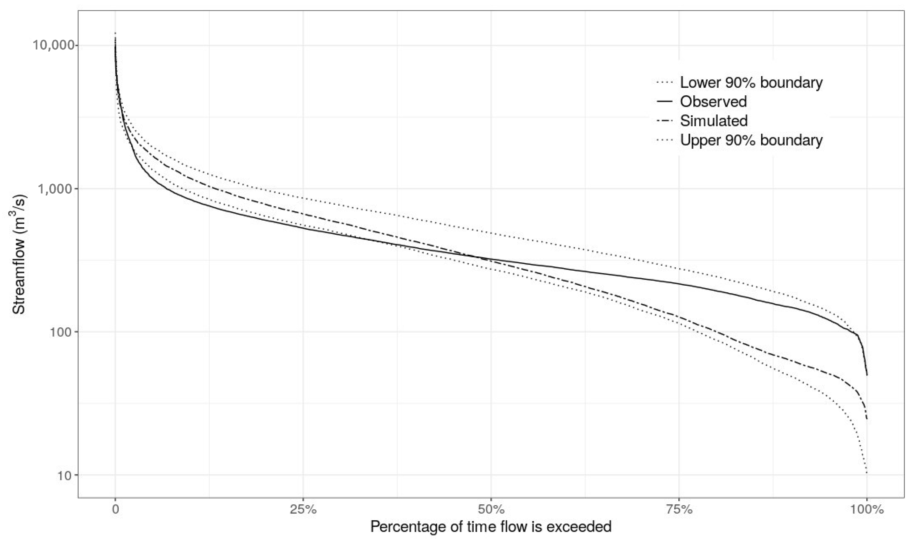
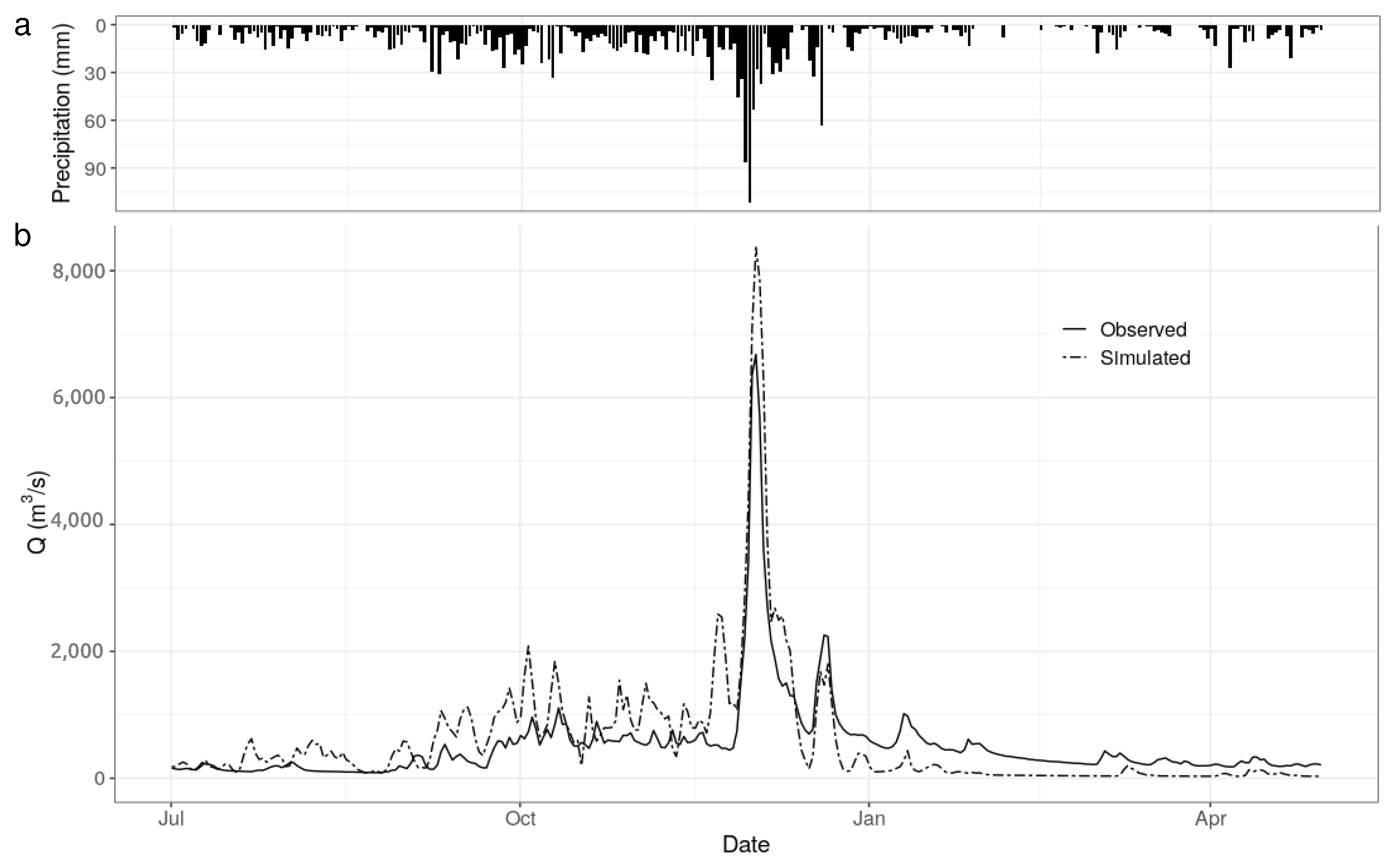
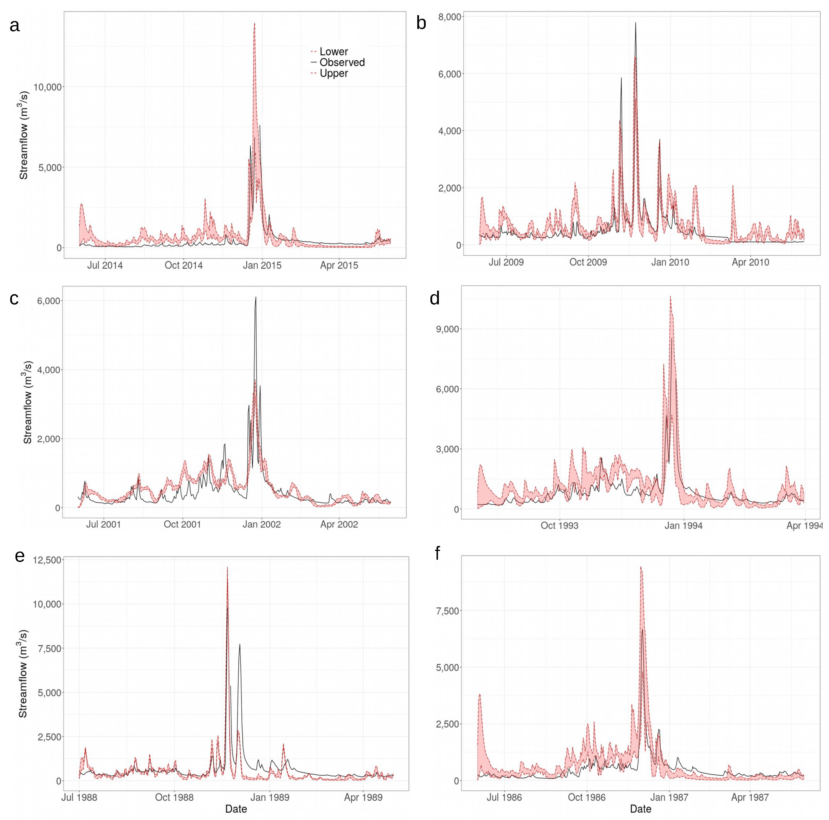
3.1. Streamflow Simulation and Model Performance

The 32 years of data simulated are presented in Figure 2 in terms of the Flow Duration Curve (FDC). The simulated line is from the highest ranked parameter, which returns $NSE$ = 0.42. The 90% upper and lower boundary are weighted based on the rejection threshold $NSE$ = 0.3. Low flows up to the 48% percentile exceedence are underestimated by the simulation while flows higher than 35% percentile exceedence is overestimated even by the lower 90% boundary. Overall, 25% of the measurement falls within the GLUE uncertainty boundary. The model FDC lines decline steeper than the observed one, which indicates the model produces higher surface flow than subsurface flow—the slope defines the characteristic- [58]. The model suggests that the flow is overestimating high flow and underestimating low flow. It maintains water balance—of precipitation, evaporation and discharge—in producing the surface runoff while the subsurface flow and storage are defined by the parameters. The underestimating of the subsurface flow in this case is the result of applying homogeneous parameters to the catchment. However, the variability of soil permeability represented by $T_0$ and $SZM$ in terms of nonmonotic exponential decline is difficult to define in the TOPMODEL structure and in parameterisation [26].

The flatter FDC of the observed streamflow compared to the simulation suggests the stream to be heavily dominated by subsurface flow which is not well captured by the model. This result corroborates the poorer model performance in groundwater-dominated catchments in the application across Great Britain [14]. Groundwater layers are observed to occur in the catchment affecting the subsurface flow. Based on the simplified hydrogeological map of the Peninsular Malaysia [59,60], sandstone and volcanic rock aquifers surrounded by igneous rock aquifers underlie the Kelantan catchment. These groundwater layers, particularly from upstream areas, play a vital role in controlling the low flow [61] derived from subsurface flow, which is addressed in the model as saturated fluxes defined by the parameters $SZM$ and the saturated transmissivity $T_0$ constraint to $S_{max}$ value. The homogeneous parameter applied in the current work does not consider the spatial variability of the groundwater layer. The ranged values assigned to the parameters do not represent the layer variability but instead are for the uncertainty computation. This suggests that better representation of groundwater recharge within the model is needed to improve the subsurface flow and supports the previous argument for the improvement of the groundwater dynamics [14].

The simulation result of the highest ranked parameter set is plotted for one peak of year 1986–1987, presented in Figure 3. Graphically the simulated streamflow is able to locate the fluctuations of the observed peaks. Along the 32-year simulation, 11 of the highest peak events are underestimated while the rest are overestimated. In both cases, the model simulation overestimates low flow before the peak but fall below the observed line after the peak recession. Since the stormflow strongly depends on the antecedent moisture [62], the low flow overestimation before the peaks are suspected to be due to the initial soil moisture value during dry period subjected to parameters $S{r}_{max}$, $S{R}_{init}$, $S_{max}$. The deep recession after the peak is due to the transmissivity exponential function, where the parameter $Szm$ controls the fall of the line. Meanwhile, the underestimation after the peaks is due to the soil state of the wet period.

The model performance evaluation returns $NSE$ = 0.42, $R^2$ = 0.47, $RMSE$ = 508.15 m${}^3$/s and $PBIAS$ = −8.8. The $NSE$ and the $R^2$ below 0.5 are considered as not satisfactory for daily streamflow simulation [63,64]. The magnitude of the $RMSE$ is also evidence of the poor model performance. However, $PBIAS$ being less than 10% is considered to be a good rating [64], whereas the negative value indicates the model overestimation bias [64,65]. In many modeling practices, these measures could justify a model be rejected. However, since the model here is aimed as a tool to gain a better understanding of the hydrological processes in the system, these patterns in the result help identify the need for the most relevant data and for the model to be further investigated.

It is inevitable that the driving data contains errors to which the uncertainty analysis is applied and parameter identification can only compensate to some level. The precipitation data from the 10 stations contain missing data of up to 15% while the streamflow observation data for the 32-year period contains 7% missing data, which may be affecting the analysis. Analysis of the water balance in the observation data set reveals that runoff constitutes 45% of the rainfall, whereas evapotranspiration makes up 49%, leaving the remaining 6% to be in storage. This suggests underestimation of rainfall within the input, which may be contributing to the modeling accuracy. Furthermore, the point rainfall is interpolated over the catchment area which may introduce additional uncertainty. The simulated fluxes indicate 50% runoff, 5% higher than that of the observed, leaving only 1% stored. Additionally, there is also a possibility of error in the GLEAM product of evapotranspiration used. It has been globally validated, but not locally corrected, for Peninsular Malaysia. Past work looking into bias and correlation with the in situ measurements of the GLEAM products in temperate countries has shown a bias of 10–30% in Switzerland [66] and correlation of 0.76 in The Netherlands [67].

The result of segmented simulation for wet periods having peaks over 6000 m${}^3$/s within the 32 years time length is tabulated in

Table 2. The segmented simulation result of peaks over 32 years.

Peak	Simulation Range (Year-Month)	Rainfall-Runoff Ratio (Q/P)	Highest Recorded Peak (m3/s)	Numerical Goodness of Fit for the Highest Rank of Parameter Set				Measurement to Fall inside the GLUE Uncertainty Limits (%)
				$\mathit{N}\mathit{S}\mathit{E}$	${\mathit{R}}^{\mathbf{2}}$	$\mathit{R}\mathit{M}\mathit{S}\mathit{E}$	$\mathit{P}\mathit{B}\mathit{I}\mathit{A}\mathit{S}$
1	2014-06/2015-05	0.40	7613.5	0.68	0.74	448.18	−21.0	14.52
2	2012-06/2013-03	0.36	6215.5	0.17	0.34	826.43	−49.6	NA
3	2009-06/2010-05	0.50	7786.0	0.70	0.75	423.43	−18.5	28.76
4	2007-06/2008-05	0.67	8028.4	0.25	0.62	638.94	6.4	NA
5	2001-06/2002-05	0.50	6111.8	0.40	0.64	392.20	−14.1	13.97
6	1993-08/1994-03	0.57	8533.7	0.72	0.75	478.00	−12.8	38.68
7	1988-07/1989-04	0.64	9775.1	0.32	0.48	772.83	30.5	17.10
8	1986-06/1987-05	0.45	6680.5	0.78	0.81	434.26	−16.0	23.83

. The length of the simulation range varies based on data quality considerations. The eight (8) peaks of data are numbered based on the sequential year. Similar rejection criteria of $NSE$ 0.3 is applied. Of the eight peaks, only two are rejected as being nonbehavioral, that is, none of the measurements fall inside the GLUE uncertainty limits. Meanwhile four peaks, Peak 1, 3, 6, 8, perform with a satisfying result, producing $NSE$ > 0.6, $R^2$ > 0.7. However, the measurement to fall inside the uncertainty limit is still below 50%. Although it is behavioral and the $NSE$ being over the rejection criteria, the model still poorly captures the system behavior. Lastly, for the remaining two peaks, though considered as behavioral, the performance results are very poor being $NSE$ 0.4 and 0.32, while $R^2$ 0.64 and 0.48, consecutively. The magnitude of the $RMSE$ also indicates the poor performance of the model. Meanwhile, the $PBIAS$ returns a varied result of positive and negative values that is underestimating and overestimating. Peak two and peak four having the lowest and the highest rainfall-runoff ratios, 0.36 and 0.67 consecutively, are rejected because the model is non behavioral. The other 6 peaks, with 4 peaks returning $NSE$ > 0.5 and 2 peaks returning $NSE$ < 0.5, are accepted as behavioral.

The six segmented behavioral model simulation plots are presented in Figure 4. Of special note for Peak 1, Figure 4a, it includes the year 2014 characterized by a big flood event reported [34,68] as the highest peak since year 1967 [69]. The recorded data, however, contains missing data at the peak event, which captured the highest amount of only 7613.5 m³/s. A study of flood risk in the Kelantan catchment between 1992 to 2014 showed that the maximum discharge at the Guillemard station is 12,900 m³/s [70]. That is, should the missing record of the peak value approximate 12,900 m³/s the simulation does indeed come close to representing the peak. Referring to the segmented simulation presented in Figure 4, the model prediction returning $NSE$ below 0.5 are for peak events 5 and 7, Figure 4c,e, while the better simulations returning $NSE$ above 0.5 are Peak 1, 3, 6, 8 as presented in Figure 4a,b,d,f. Simulation (c) fails to predict the magnitude of the two highest peaks. The deviation before the peak is also high but the recession does fit the observed. Meanwhile, simulation (e) overpredicts the first highest peak and fails to capture the second one completely. The deviation before the peak is small but the recession is simulated more quickly than the observed. In both events, the performance measures are similar but the indications of model underperformance are different. Hence, the reason why the model is able to predict some peaks but not others could not be inferred.

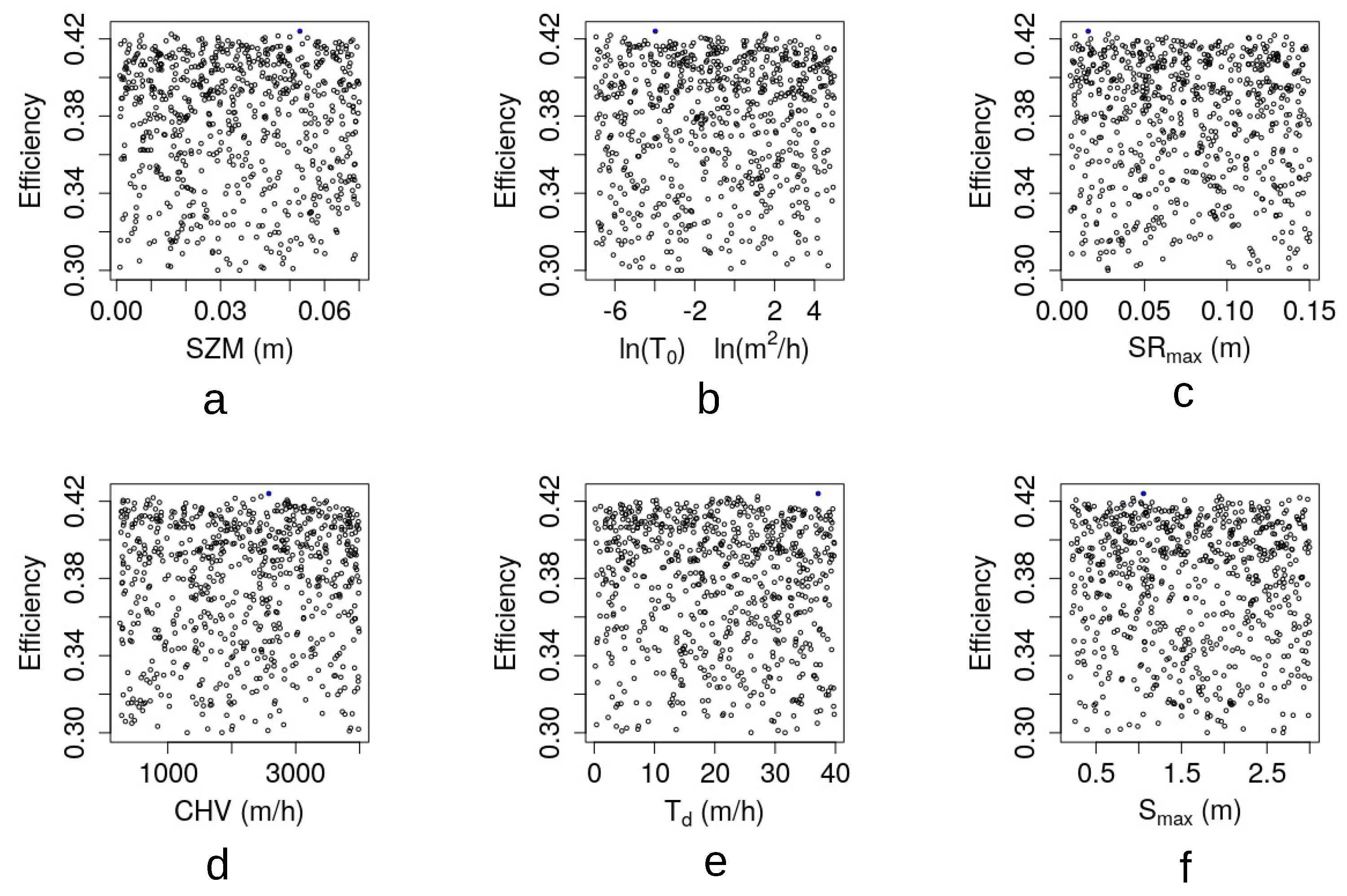
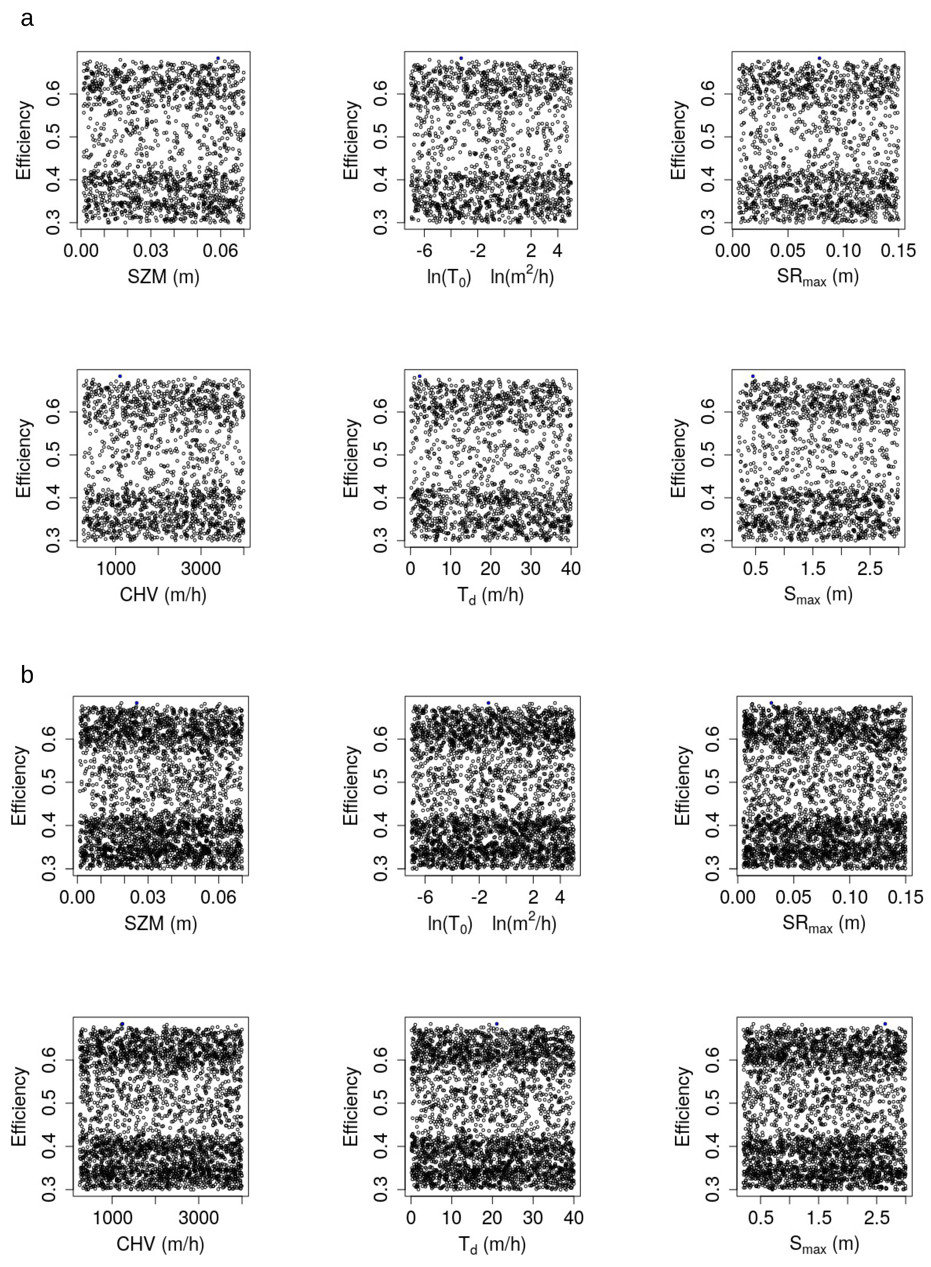
3.2. Analysis of Model Parameters

In spite of general model poor performance, there are sets of behavioral parameters that indicate the equifinality of the model toward the system. The behavioral parameter distribution are plotted using a scatterplot, presented in Figure 5 for the 32 year period simulated. It can be seen that the scatterplots do not appear to have any pattern; instead, the efficiency appear random across the parameter values. This supports the prior FDC discussion that the model parameters do not represent the system well because they are applied homogeneously throughout the catchment.

As for the segmented simulations, all the behavioral peaks addressed show similar nonidentifiablity of the parameters. Only Peak 1’s plot is presented in Figure 6. Previous studies of TOPMODEL and dynamic TOPMODEL application have suggested that the most sensitive parameters are $SZM$, $T_0$, and $S{r}_{max}$[12,13,71], which is not the case here even though the set of parameters are being behavioral given the acceptable model threshold of $NSE$ 0.3. It is important to note, however, that some of the segmented simulations do return a better performance of $NSE$, which indicates better parameter sets. A higher number (i.e., 10,000 sets) is also represented in the scatterplot Figure 6b, which also shows that it does not affect the scatter pattern.

The nonidentifiability of parameters is suspected due to the large scale of the catchment where heterogeneity is inevitable. A semidistributed HRU approach could represent a better spatial process of the system compared to a lumped or a black box model. However, actual improvement in process understanding can only be achieved when the parameters can be identified at more local scales. In the Kelantan catchment, more significant groundwater recharge could be expected in the upstream forested areas. However, given that the model is calibrated at a single point, it generalizes all infiltration processes across the entire catchment and is unable to accurately represent the spatial variability of the hydrological processes. This requires a modification of the model structure and additional parameters definition. Extensive field measurements may be required to support calibration of spatial varying parameters, otherwise the parameter space becomes too large. The effort is more applicable to small catchment study such as the TOPMODEL application in small Baru River Catchment in Malaysian Borneo [27] and the field based local scale calibration of HEC-HMS in Aspio river Italy [72].

4. Conclusions

In this work, the DECIPHeR framework was tested in a representative tropical forested catchment. In general the model’s ability to simulate the system is reasonable but limited based on performance measures alone. However, as an interactive framework for understanding the hydrological processes and the modeling of the system, DECIPHeR enabled identification of further advances to be made.

Underperformance of the model to represent the system due to low flows can be observed from both the continuous 32 years period and the segmented event simulations after the peak recession. The FDC curve further confirms overall low flow estimation. The simulation before and after the peaks suggests that soil controls on runoff may be responsible for the deviations from the observed streamflow. This is supported by the ability of the model to correctly capture the timings of large and small peaks. The behavioral model parameters being insensitive and unidentifiable may indicate the spatial heterogeneity of the parameters, which is yet to be addressed by the model framework; instead a homogeneous parameter assumed to fit the entire catchment may only work for small catchments. These are the considerations for further analysis of the model application introducing new spatial layers for representing soil and landcover heterogeneity, modification in the model structure to differentiate processes for different landcover and soils, and application of the model at smaller subcatchments.

The conclusions of this study are nevertheless subjected to several limitations of the study. Firstly, the 32 year period (1985–2016) of simulations based on data availability only allows inspection of the model during the particular time period. Secondly, there may be errors introduced due to interpolated rainfall, as well as the use of the satellite-based $PET$ from GLEAM, which is a global dataset without local bias correction.

References

1. Sivapalan, M.; Takeuchi, K.; Franks, S.; Gupta, V.; Karambiri, H.; Lakshmi, V.; Liang, X.; McDonnell, J.; Mendiondo, E.; O’connell, P.; et al. IAHS Decade on Predictions in Ungauged Basins (PUB), 2003–2012: Shaping an exciting future for the hydrological sciences. Hydrol. Sci. J. 2003, 48, 857–880. [Google Scholar] [CrossRef] [Green Version]
2. Silberstein, R. Hydrological models are so good, do we still need data? Environ. Model. Softw. 2006, 21, 1340–1352. [Google Scholar] [CrossRef]
3. Singh, V.P.; Frevert, D.K. Mathematical Models of Small Watershed Hydrology and Applications; Water Resources Publication: Lone Tree, CO, USA, 2002. [Google Scholar]
4. Merz, R.; Parajka, J.; Blöschl, G. Scale effects in conceptual hydrological modeling. Water Resour. Res. 2009, 45. [Google Scholar] [CrossRef]
5. Devia, G.K.; Ganasri, B.; Dwarakish, G. A review on hydrological models. Aquat. Procedia 2015, 4, 1001–1007. [Google Scholar] [CrossRef]
6. Sitterson, J.; Knightes, C.; Parmar, R.; Wolfe, K.; Avant, B.; Muche, M. An overview of rainfall-runoff model types. In International Congress on Environmental Modelling and Software; Brigham Young University: Provo, UT, USA, 2018. [Google Scholar]
7. Beven, K.J. Rainfall-Runoff Modelling: The Primer; John Wiley & Sons: Oxford, UK, 2011. [Google Scholar]
8. Uhlenbrook, S.; Seibert, J.; Leibundgut, C.; Rodhe, A. Prediction uncertainty of conceptual rainfall-runoff models caused by problems in identifying model parameters and structure. Hydrol. Sci. J. 1999, 44, 779–797. [Google Scholar] [CrossRef]
9. Fenicia, F.; Kavetski, D.; Savenije, H.H. Elements of a flexible approach for conceptual hydrological modeling: 1. Motivation and theoretical development. Water Resour. Res. 2011, 47. [Google Scholar] [CrossRef]
10. Seibert, J. Conceptual Runoff Models-Fiction or Representation of Reality; Acta Universitatis Upsaliensis: Uppsala, Sweden, 1999. [Google Scholar]
11. Campling, P.; Gobin, A.; Beven, K.; Feyen, J. Rainfall-runoff modelling of a humid tropical catchment: The TOPMODEL approach. Hydrol. Process. 2002, 16, 231–253. [Google Scholar] [CrossRef]
12. Beven, K.; Freer, J. A dynamic topmodel. Hydrol. Process. 2001, 15, 1993–2011. [Google Scholar] [CrossRef]
13. Metcalfe, P.; Beven, K.; Freer, J. Dynamic TOPMODEL: A new implementation in R and its sensitivity to time and space steps. Environ. Model. Softw. 2015, 72, 155–172. [Google Scholar] [CrossRef] [Green Version]
14. Coxon, G.; Freer, J.; Lane, R.; Dunne, T.; Knoben, W.J.; Howden, N.J.; Quinn, N.; Wagener, T.; Woods, R. DECIPHeR v1: Dynamic fluxEs and ConnectIvity for Predictions of HydRology. Geosci. Model Dev. 2019, 12. [Google Scholar] [CrossRef] [Green Version]
15. Buytaert, W.; Reusser, D.; Krause, S.; Renaud, J.P. Why can’t we do better than Topmodel? Hydrol. Process. Int. J. 2008, 22, 4175–4179. [Google Scholar] [CrossRef]
16. Pechlivanidis, I.G.; Jackson, B.M.; Mcintyre, N.R.; Wheater, H.S. Catchment scale hydrological modelling: A review of model types, calibration approaches and uncertainty analysis methods in the context of recent developments in technology and applications. Glob. NEST J. 2011, 13, 193–214. [Google Scholar]
17. Stedinger, J.R.; Vogel, R.M.; Lee, S.U.; Batchelder, R. Appraisal of the generalized likelihood uncertainty estimation (GLUE) method. Water Resour. Res. 2008, 44. [Google Scholar] [CrossRef]
18. Montanari, A. What do we mean by ‘uncertainty’? The need for a consistent wording about uncertainty assessment in hydrology. Hydrol. Process. Int. J. 2007, 21, 841–845. [Google Scholar] [CrossRef]
19. Beven, K.; Freer, J. Equifinality, data assimilation, and uncertainty estimation in mechanistic modelling of complex environmental systems using the GLUE methodology. J. Hydrol. 2001, 249, 11–29. [Google Scholar] [CrossRef]
20. Beven, K. Environmental Modelling: An Uncertain Future; Routledge: London, UK, 2010. [Google Scholar]
21. Page, T.; Beven, K.J.; Freer, J.; Neal, C. Modelling the chloride signal at Plynlimon, Wales, using a modified dynamic TOPMODEL incorporating conservative chemical mixing (with uncertainty). Hydrol. Process. Int. J. 2007, 21, 292–307. [Google Scholar] [CrossRef]
22. Montanari, A. Large sample behaviors of the generalized likelihood uncertainty estimation (GLUE) in assessing the uncertainty of rainfall-runoff simulations. Water Resour. Res. 2005, 41. [Google Scholar] [CrossRef]
23. Gil, E.G.; Tobón, C. Hydrological modelling with TOPMODEL of Chingaza páramo, Colombia. Rev. Fac. Nac. Agron. Medellín 2016, 69, 7919–7933. [Google Scholar]
24. Buytaert, W.; Beven, K. Models as multiple working hypotheses: Hydrological simulation of tropical alpine wetlands. Hydrol. Process. 2011, 25, 1784–1799. [Google Scholar] [CrossRef]
25. Suliman, A.H.A.; Katimon, A.; Darus, I.Z.M.; Shahid, S. TOPMODEL for streamflow simulation of a tropical catchment using different resolutions of ASTER DEM: Optimization through response surface methodology. Water Resour. Manag. 2016, 30, 3159–3173. [Google Scholar] [CrossRef]
26. Chappell, N.A.; Bidin, K.; Sherlock, M.; Lancaster, J. Parsimonious spatial representation of tropical soils within dynamic, rainfall-runoff models. In Forests, Water and People in the Humid Tropics; Cambridge University Press: Cambridge, UK, 2004; pp. 756–769. [Google Scholar]
27. Chappell, N.A.; Franks, S.W.; Larenus, J. Multi-scale permeability estimation for a tropical catchment. Hydrol. Process. 1998, 12, 1507–1523. [Google Scholar] [CrossRef] [Green Version]
28. Peters, N.E.; Freer, J.; Beven, K. Modelling hydrologic responses in a small forested catchment (Panola Mountain, Georgia, USA): A comparison of the original and a new dynamic TOPMODEL. Hydrol. Process. 2003, 17, 345–362. [Google Scholar] [CrossRef]
29. Suliman, A.H.A.; Gumindoga, W.; Katimon, A. Semi-distributed rainfall-runoff modeling utilizing ASTER DEM in Pinang Catchment of Malaysia. Sains Malays. 2014, 43, 1379–1388. [Google Scholar]
30. Gumindoga, W.; Rientjes, T.; Haile, A.; Dube, T. Predicting streamflow for land cover changes in the Upper Gilgel Abay River Basin, Ethiopia: A TOPMODEL based approach. Phys. Chem. Earth Parts A/B/C 2014, 76, 3–15. [Google Scholar] [CrossRef]
31. Arenas-Bautista, M.C.; Arboleda-Obando, P.F.; Duque-Gardeazabal, N.; Saavedra-Cifuentes, E.; Donado, L.D. Hydrological Modeling in Tropical Regions via TopModel. Study Case: Central Sector of the Middle Magdalena Valley-Colombia. Preprints 2018. [Google Scholar] [CrossRef] [Green Version]
32. Takeuchi, K.; Ao, T.; Ishidaira, H. Introduction of block-wise use of TOPMODEL and Muskingum-Cunge method for the hydroenvironmental simulation of a large ungauged basin. Hydrol. Sci. J. 1999, 44, 633–646. [Google Scholar] [CrossRef]
33. Magome, J.; Gusyev, M.; Hasegawa, A.; Takeuchi, K. River discharge simulation of a distributed hydrological model on global scale for the hazard quantification. In Proceedings of the 21st International Congress on Modelling and Simulation (MODSIM2015), Broadbeach, Australia, 29 November–4 December 2015; pp. 1593–1599. [Google Scholar]
34. Jaafar, A.S.; Sidek, L.M.; Basri, H.; Zahari, N.M.; Jajarmizadeh, M.; Noor, H.M.; Osman, S.; Mohammad, A.H.; Azad, W.H. An overview: Flood catastrophe of Kelantan watershed in 2014. In ISFRAM 2015; Springer: Singapore, 2016; pp. 17–29. [Google Scholar] [CrossRef]
35. Butler, R. High Deforestation Rates in Malaysian States Hit by Flooding. Mongabay, 19 January 2015. [Google Scholar]
36. Shakirah, J.A.; Sidek, L.; Hidayah, B.; Nazirul, M.; Jajarmizadeh, M.; Ros, F.; Roseli, Z. A Review on Flood Events for Kelantan River Watershed in Malaysia for Last Decade (2001–2010). In Proceedings of the IOP Conference Series: Earth and Environmental Science, Putrajaya, Malaysia, 23–25 February 2016; IOP Publishing Ltd.: Bristol, UK, 2016; Volume 32, p. 012070. [Google Scholar] [CrossRef]
37. Ahmad Shafuan, M.F. Runoff Estimation Using SCS CN Method For Kelantan River Basin. In Proceedings of the International Conference on Water Resources, Bayview Hotel, Langkawi, Malaysia, 24–25 November 2015. [Google Scholar] [CrossRef]
38. Hafiz, I.; Sidek, L.; Basri, H.; Fukami, K.; Hanapi, M.; Livia, L.; Jaafar, A. Integrated flood analysis system (IFAS) for Kelantan river basin. In Proceedings of the 2014 IEEE 2nd International Symposium on Telecommunication Technologies (ISTT), Langkawi, Malaysia, 24–26 November 2014; pp. 159–162. [Google Scholar]
39. Saadatkhah, N.; Tehrani, M.H.; Mansor, S.; Khuzaimah, Z.; Kassim, A.; Saadatkhah, R. Impact assessment of land cover changes on the runoff changes on the extreme flood events in the Kelantan River basin. Arab. J. Geosci. 2016, 9, 687. [Google Scholar] [CrossRef]
40. Basarudin, Z.; Adnan, N.A.; Latif, A.R.A.; Tahir, W.; Syafiqah, N. Event-based rainfall-runoff modelling of the Kelantan River Basin. In Proceedings of the IOP Conference Series: Earth and Environmental Science, Kuching, Malaysia, 26–29 August 2013; Volume 18, p. 012084. [Google Scholar]
41. Adnan, N.A.; Atkinson, P. Disentangling the effects of long-term changes in precipitation and land use on hydrological response in a monsoonal catchment. J. Flood Risk Manag. 2018, 11, S1063–S1077. [Google Scholar] [CrossRef] [Green Version]
42. Woodward, D.E.; Hawkins, R.H.; Hjelmfelt, A.; Van Mullem, J.; Quan, Q.D. Curve number method: Origins, applications and limitations. In Proceedings of the US Geological Survey Advisory Committee on Water Information–Second Federal Interagency Hydrologic Modeling Conference, Las Vegas, NV, USA, 28 July–1 August 2002. [Google Scholar]
43. Nasr, A.; Bruen, M. Development of neuro-fuzzy models to account for temporal and spatial variations in a lumped rainfall–runoff model. J. Hydrol. 2008, 349, 277–290. [Google Scholar] [CrossRef] [Green Version]
44. Shamseldin, A.Y.; O’CONNOR, K.M.; Nasr, A.E. A comparative study of three neural network forecast combination methods for simulated river flows of different rainfall—Runoff models. Hydrol. Sci. J. 2007, 52, 896–916. [Google Scholar] [CrossRef]
45. Fu, M.; Fan, T.; Ding, Z.; Salih, S.Q.; Al-Ansari, N.; Yaseen, Z.M. Deep Learning Data-Intelligence Model Based on Adjusted Forecasting Window Scale: Application in Daily Streamflow Simulation. IEEE Access 2020, 8, 32632–32651. [Google Scholar] [CrossRef]
46. Wong, C.; Venneker, R.; Uhlenbrook, S.; Jamil, A.; Zhou, Y. Variability of rainfall in Peninsular Malaysia. Hydrol. Earth Syst. Sci. Discuss. 2009, 6, 5471–5503. [Google Scholar] [CrossRef] [Green Version]
47. Jabatan Penerangan. Available online: http://pmr.penerangan.gov.my (accessed on 10 June 2017).
48. USGS. Earth Explorer. SRTM/Shuttle Radar Topography Mission 1 Arc-Second Digital Terrain Elevation Data-Global. Available online: https://earthexplorer.usgs.gov/ (accessed on 10 November 2017).
49. Ludwig, R.; Schneider, P. Validation of digital elevation models from SRTM X-SAR for applications in hydrologic modeling. ISPRS J. Photogramm. Remote Sens. 2006, 60, 339–358. [Google Scholar] [CrossRef]
50. Martens, B.; Gonzalez Miralles, D.; Lievens, H.; Van Der Schalie, R.; De Jeu, R.A.; Fernández-Prieto, D.; Beck, H.E.; Dorigo, W.; Verhoest, N. GLEAM v3: Satellite-based land evaporation and root-zone soil moisture. Geosci. Model Dev. 2017, 10, 1903–1925. [Google Scholar] [CrossRef] [Green Version]
51. Gonzalez Miralles, D.; Holmes, T.; De Jeu, R.; Gash, J.; Meesters, A.; Dolman, A. Global land-surface evaporation estimated from satellite-based observations. Hydrol. Earth Syst. Sci. 2011, 15, 453–469. [Google Scholar] [CrossRef] [Green Version]
52. Beven, K.J.; Kirkby, M.J. A physically based, variable contributing area model of basin hydrology/Un modèle à base physique de zone d’appel variable de l’hydrologie du bassin versant. Hydrol. Sci. J. 1979, 24, 43–69. [Google Scholar] [CrossRef] [Green Version]
53. Beven, K. TOPMODEL: A critique. Hydrol. Process. 1997, 11, 1069–1085. [Google Scholar] [CrossRef]
54. Beven, K.; Binley, A. The future of distributed models: Model calibration and uncertainty prediction. Hydrol. Process. 1992, 6, 279–298. [Google Scholar] [CrossRef]
55. Shen, Z.; Chen, L.; Chen, T.; Di Baldassarre, G. Analysis of parameter uncertainty in hydrological and sediment modeling using GLUE method: A case study of SWAT model applied to Three Gorges Reservoir Region, China. Hydrol. Earth Syst. Sci. 2012, 16, 121–132. [Google Scholar] [CrossRef] [Green Version]
56. Harmel, R.D.; Smith, P.K.; Migliaccio, K.W. Modifying goodness-of-fit indicators to incorporate both measurement and model uncertainty in model calibration and validation. Trans. ASABE 2010, 53, 55–63. [Google Scholar] [CrossRef]
57. Freer, J.; Beven, K.; Ambroise, B. Bayesian estimation of uncertainty in runoff prediction and the value of data: An application of the GLUE approach. Water Resour. Res. 1996, 32, 2161–2173. [Google Scholar] [CrossRef]
58. Searcy, J.K.; Hardison, C.H. Double-Mass Curves; Number 1541; US Government Printing Office: Washington, DC, USA, 1960.
59. Heng, C.L. Groundwater utilisation and management in Malaysia. In Proceedings of the 41 st CCOP Annual Session, Tsukuba, Japan, 15–18 November 2004; p. 83. [Google Scholar]
60. Chong, F.; Tan, D.N. Hydrogeological Activities in Peninsular Malaysia and Sarawak; Geological Society of Malaysia: Kuala Lumpur, Malaysia, 1986; Volume 2, pp. 827–842. [Google Scholar]
61. Brutsaert, W. Long-term groundwater storage trends estimated from streamflow records: Climatic perspective. Water Resour. Res. 2008, 44. [Google Scholar] [CrossRef]
62. Noguchi, S.; Nik, A.R.; Yusop, Z.; Tani, M.; Sammori, T. Rainfall-runoff responses and roles of soil moisture variations to the response in tropical rain forest, Bukit Tarek, Peninsular Malaysia. J. For. Res. 1997, 2, 125–132. [Google Scholar] [CrossRef]
63. Moriasi, D.N.; Gitau, M.W.; Pai, N.; Daggupati, P. Hydrologic and water quality models: Performance measures and evaluation criteria. Trans. ASABE 2015, 58, 1763–1785. [Google Scholar]
64. Moriasi, D.N.; Arnold, J.G.; Van Liew, M.W.; Bingner, R.L.; Harmel, R.D.; Veith, T.L. Model evaluation guidelines for systematic quantification of accuracy in watershed simulations. Trans. ASABE 2007, 50, 885–900. [Google Scholar] [CrossRef]
65. Gupta, H.V.; Sorooshian, S.; Yapo, P.O. Status of automatic calibration for hydrologic models: Comparison with multilevel expert calibration. J. Hydrol. Eng. 1999, 4, 135–143. [Google Scholar] [CrossRef]
66. Freund, E.R.; Zappa, M.; Kirchner, J.W. Averaging over spatiotemporal heterogeneity substantially biases evapotranspiration rates in a mechanistic large-scale land evaporation model. Hydrol. Earth Syst. Sci 2020, 24, 5015–5025. [Google Scholar] [CrossRef]
67. Martens, B.; De Jeu, R.A.; Verhoest, N.E.; Schuurmans, H.; Kleijer, J.; Miralles, D.G. Towards Estimating Land Evaporation at Field Scales Using GLEAM. Remote Sens. 2018, 10, 1720. [Google Scholar] [CrossRef] [Green Version]
68. Alias, N.E.; Mohamad, H.; Chin, W.Y.; Yusop, Z. Rainfall analysis of the Kelantan big yellow flood 2014. J. Teknol. 2016, 78. [Google Scholar] [CrossRef] [Green Version]
69. Azlee, A. Worst floods in Kelantan, confirms NSC. Retrieved January 2015, 5, 2017. [Google Scholar]
70. Ghorbani, K.; Wayayok, A.; Abdullah, A.F. Simulation of flood risk area in Kelantan watershed, Malaysia using numerical model. J. Teknol. 2016, 78, 51–57. [Google Scholar] [CrossRef] [Green Version]
71. Freer, J.E.; McMillan, H.; McDonnell, J.; Beven, K. Constraining dynamic TOPMODEL responses for imprecise water table information using fuzzy rule based performance measures. J. Hydrol. 2004, 291, 254–277. [Google Scholar] [CrossRef]
72. Fronzi, D.; Tazioli, A. Groundwater and flood events in different hydrogeological periods: A case study in the Aspio river (Marche Region). Ital. J. Eng. Geol. Environ. 2019, 1. [Google Scholar] [CrossRef]
Figure 1. (a) Kelantan River network and catchment with rainfall and streamflow stations, (b) The Kelantan catchment location in Peninsular Malaysia.
Water 13 00317 g001
Figure 2. Flow Duration Curve plot of the 32 years observed data, simulation result of the highest rank parameter, and the GLUE uncertainty boundary.
Water 13 00317 g002
Figure 3. (a) The mean areal precipitation, (b) The observed and the simulated streamflow of the highest rank parameter set.
Water 13 00317 g003
Figure 4. The observed and the GLUE uncertainty boundary. (a) Peak 1, (b) Peak 3, (c) Peak 5, (d) Peak 6, (e) Peak 7, (f) Peak 8.
Water 13 00317 g004
Figure 5. Scatter plot of efficiency versus behavioral parameters values (a) Form of exponential decline in conductivity, (b) Effective lateral saturated transmissivity, (c) Maximum root zone storage, (d) Channel routing velocity, (e) Unsaturated zone time delay, (f) Maximum effective deficit of subsurface saturated zone, for 32 years’ simulation.
Water 13 00317 g005
Figure 6. Scatter plot of efficiency versus behavioral parameters values for Peak 1 (a) 5000 simulations, (b) 10,000 simulations.
Water 13 00317 g006