
Secondary Currents with Scour Hole at Grade Control Structures


Department of Civil, Environmental, Land, Building Engineering and Chemistry, Polytechnic University of Bari, Via E. Orabona 4, 70125 Bari, Italy
*
Author to whom correspondence should be addressed.
Water 2021, 13(3), 319; https://doi.org/10.3390/w13030319
Submission received: 25 December 2020
/
Revised: 22 January 2021
/
Accepted: 23 January 2021
/
Published: 28 January 2021
(This article belongs to the Special Issue Flow Hydrodynamic in Open Channels: Interaction with Natural or Man-Made Structures)
Abstract
:Most studies on local scouring at grade control structures have principally focused on the analysis of the primary flow field, predicting the equilibrium scour depth. Despite the numerous studies on scouring processes, secondary currents were not often considered. Based on comprehensive measurements of flow velocities in clear water scours downstream of a grade control structure in a channel with non-cohesive sediments, in this study, we attempted to investigate the generation and turbulence properties of secondary currents across a scour hole at equilibrium condition. The flow velocity distributions through the cross-sectional planes at the downstream location of the maximum equilibrium scour depth clearly show the development of secondary current cells. The secondary currents form a sort of helical-like motion, occurring in both halves of the cross-section in an axisymmetric fashion. A detailed analysis of the turbulence intensities and Reynolds shear stresses was carried out and compared with previous studies. The results highlight considerable spatial heterogeneities of flow turbulence. The anisotropy term of normal stresses dominates the secondary shear stress, giving the impression of its crucial role in generating secondary flow motion across the scour hole. The anisotropy term shows maximum values near both the scour mouth and the scour bed, caused, respectively, by the grade control structure and the sediment ridge formation, which play fundamental roles in maintaining and enhancing the secondary flow motion.
1. Introduction
The presence of natural or man-made structures on riverbeds plays an important role in the evolution of river morphology and sediment entrainment. Flow turbulence properties and secondary currents play a crucial role in sediment transport, and, in turn, suspended particle motion influences turbulence, such as Reynolds shear stress and velocity [1]. In addition to the fluid–particle interactions, which definitely influence the flow velocity distribution, the fluid–structure interactions, i.e., with natural vegetations, riverbed debris, bridge piers and abutments, sills, sluice gates, spillways, weirs, spur dikes, off-shore platforms, wind turbines, energy converters, etc., cause additional complex effects on the flow hydrodynamic characteristics. Local scouring is produced due to these complex flow patterns occurring in the surroundings of such structures. The local scouring process has attracted the attention and interest of many scientists for decades [2,3,4,5,6,7,8,9,10,11,12,13,14,15,16,17,18].
Experimental studies on the scouring process at grade control structures (GCSs) in riverbeds [3,5,9,17,18] showed that the scour often developed downstream of the structure. The extension of the scour hole is strongly influenced by the properties of the incoming flow, which is usually a two-dimensional jet-like flow. Owing to the high velocity of the entering jet flow, a large amount of sediment erosion locally occurs downstream of the GCS, forming the scour hole. Because of the large velocity gradients among the jet flow and that in the scour pool, the jet diffuses near the bed, and is redirected at a reduced bed velocity. The equilibrium state occurs when the path of the impinging jet becomes long enough and its diffused velocity is reduced to values below the minimum value required to move the sediments [17,18]. The entering jet produces a very complex flow field in the scour hole. For structures around which the flow passes (bypassed structures), i.e., bridge piers, abutments, offshore platforms, and wind turbines, the scour profile is considerably affected by the flow turbulence structures, generated in the form of a horseshoe vortex, wake vortex, and surface roller [14].
Most studies on local scouring downstream of GCSs have essentially focused on the prediction of the maximum scour dimensions at equilibrium, especially the maximum scour depth and the maximum length. For the sake of simplicity, in these studies, flows have been analyzed in the plane of flow symmetry (along the channel axis), neglecting the effect of the wall-normal velocity component. However, flows within scour holes, regardless of the GCS’s geometry, are three-dimensional, and therefore, secondary currents can occur in some cross-sections of the scour hole. Secondary currents represent circulation of fluids around the axis of the primary flow [19].
In open channel flows, secondary currents affect the distribution of bed shear stress, Reynolds stress, and turbulence intensities across the channel [20]. In large channels, the secondary currents consist of a series of counter-rotating cells through the sectional planes. Between the cells, upwelling and downwelling alternating movement zones may occur, which extend over the entire water column. Secondary current cells often generate a sort of undulating bottom shear stress distribution in the transverse direction, affecting the whole depth-flow field and the free-surface flow pattern [20,21]. According to Albayrak and Lemmin [20], the dynamics of secondary currents are strongly affected by the channel aspect ratio. The authors [20] observed that the number of secondary current cells changes proportionally with the aspect ratio. Within the range of their experimental conditions, Albayrak and Lemmin [20] also argued that, for a given aspect ratio, the number of secondary current cells is not affected by changes in the Reynolds number or the Froude number. Papanicolaou et al. [22] proved that the presence of secondary currents increases the sidewall shear stress and affects the turbulent production within a channel flow.
Secondary flow circulation and scouring processes were also observed in stream confluences [23,24,25]. The increase of flow velocity due to tributary junction generates a zone of maximum scour located near the center of the confluence. This zone is characterized by dominant flow convergence and a consistent pattern of secondary circulation.
Despite the numerous studies conducted on local scouring, a lack of information regarding the structures and generation of a secondary current in scour holes has been noted in literature. The main factors generating secondary currents in straight non-circular channel flows have been and remains a topic of much discussion and conjecture. In this study, we essentially focus on the hydrodynamic characteristics of flow across scour holes developed downstream of a GCS in sand riverbeds. Thanks to several measurements of the flow velocities performed through the scour cross-section at the position of maximum equilibrium scour depth, the secondary current patterns in the scour hole were achieved. This paper aims to: (i) check the development of secondary currents in scour hole downstream of a GCS, (ii) analyze the evolution of the turbulence structure in the scour hole at the equilibrium condition, and (iii) try to understand the physical origin of secondary current cells across the equilibrium scour hole.
2. Theoretical Considerations
Sand ridges, also termed sediment strips, which are usually aligned parallel to the direction of the mean flow, have been widely observed in nature, i.e., in rivers with a bed composed of non-cohesive material, continental shelves, estuaries, and deserts [26]. These phenomena are strongly related to the development of secondary currents. In the literature (e.g., [20,21,26]), steady secondary currents have been classified into two categories: (i) secondary currents of the first kind (skew-induced stream-wise vorticity), taking origin from mean flow, but driven by curvature effect, and (ii) secondary currents that are generated by anisotropy of flow turbulence.
For steady flow and incompressible fluid, the time-averaged continuity and Navier–Stokes equations are (using index notation):
where xi and xj = (x, y, z) is the direction tensor, Ui and Uj = (U, V, W) is the time-averaged velocity tensor, in which U, V, and W are the velocity along x, y, and z, respectively, ρ is the water density, p is the pressure force, ν is the water kinematic viscosity, gi is the gravitational acceleration tensor, τij = −U′iU′j is the shear stress tensor, and U′iU′j is the time-averaged shear stress of U′iU′j(t) over the length of the time series. The instantaneous velocity is defined as ui(t) = Ui + U′i(t), where U′i = (U′, V′, W′) is the velocity fluctuation tensor of u, v, and w, respectively.
From Equation (2), one can obtain the equation of the transport of stream-wise momentum as:
In Equation (3), I is the pressure gradient driving the flow, II indicates the convective transport of stream-wise momentum, III represents the transport due to viscous shear stresses, and IV is the transport due to turbulent stresses. The term III is generally negligible, except close to boundaries (bed and banks/walls). In the case of uniformly developed turbulent flow, ∂/∂x = 0 in the terms II, III, and IV.
Since, in this study, the channel is straight, and the anisotropy of the flow turbulence could be the source of the secondary current formation. In this case, the secondary currents (steady and incompressible flow) can be described by the stream-wise vorticity equation as:
where ,, and are the stream-wise, the span-wise, and the vertical vorticities, respectively. The term A1 in Equation (4) represents the rate of change of ωx due to the convection of fluid by the mean flow velocities: primary flow U and secondary motions V and W. The term A2 represents the tilting and stretching of the three vorticities by the gradients of the mean flow velocities. The term A3 represents the viscous diffusion of ωx. The terms A4, A5, and A6 represent the rates of change of the normal and shear stresses in the cross-section plane, which are theoretically responsible for developing and maintaining the second kind of secondary currents [27,28].
3. Experimental Set-Up
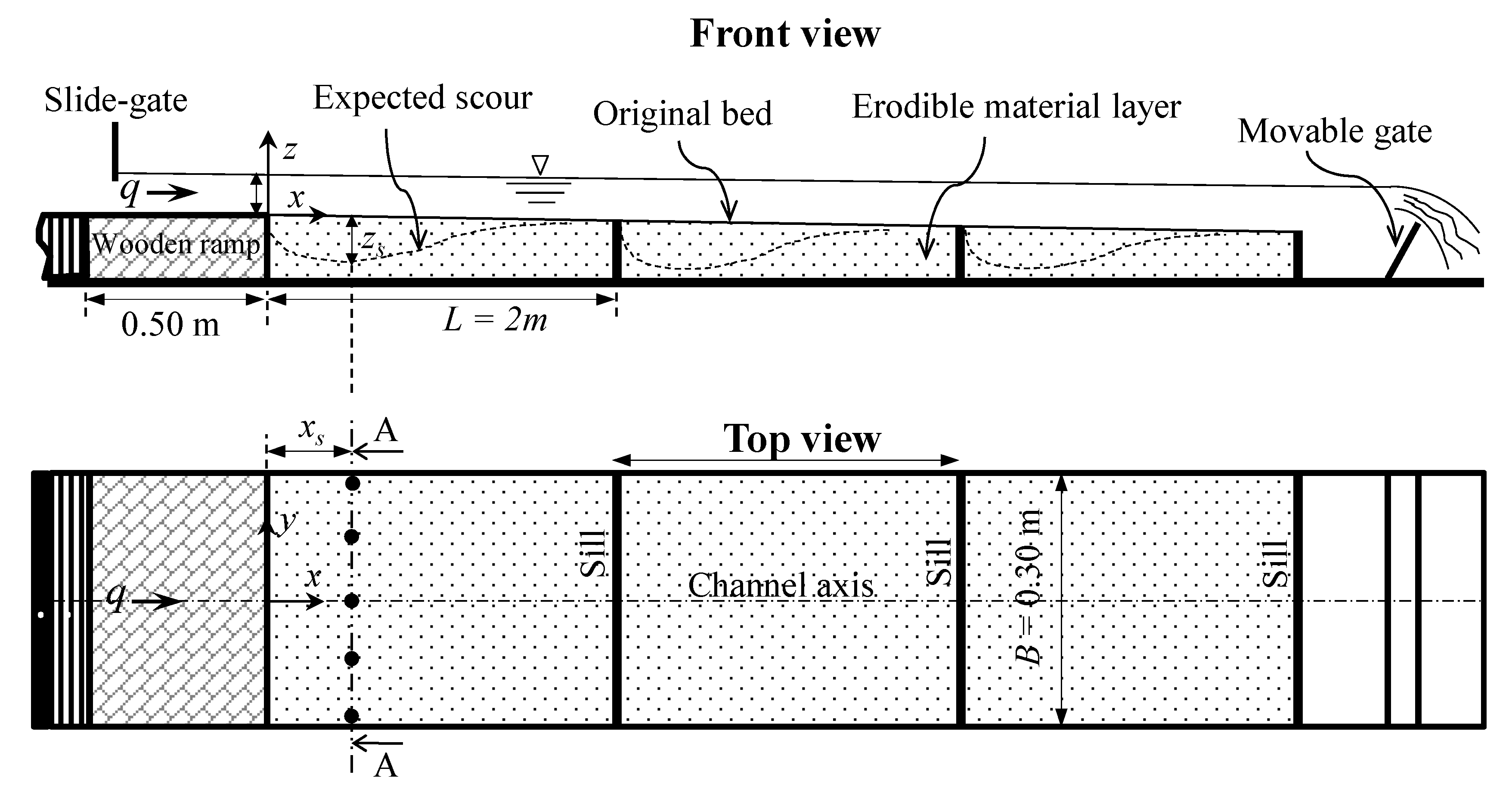
The experiments on the scour processes were carried out in a rectangular flume of closed-circuit flow at the Hydraulic Laboratory of the Mediterranean Agronomic Institute of Bari (Bari, Italy). The flume had glass sidewalls and a Plexiglas floor, allowing a good side view of the flow. It was 7.72 m long, 0.30 m wide, and 0.40 m deep. A pump with a maximum discharge of 24 L/s was used to deliver water from the laboratory sump to an upstream tank equipped with a baffle and lateral weir, maintaining a constant head upstream of a movable slide gate constructed at the inlet of the flume. The slide gate regulates channel flow discharge. To create a smooth flow transition from the upstream reservoir to the flume, a rectangular wooden ramp, playing the role of a first GCS, was installed at the inlet of the flume; it was 1.55 m long and 0.15 m thick, and of the same channel width (Figure 1). At the outlet of the flume, water was intercepted by a stilling tank, equipped with three vertical grids to stabilize water, and a triangular weir (V-notch sharp crested weir) to measure the discharge with a relative uncertainty of ± 8%. At the downstream end of the flume, a movable gate made of Plexiglas and hinged at the channel bottom was used to regulate the flow depth.
To simulate grade control structures to protect riverbeds against erosion, in this study, we used a series of sills that consisted of PVC plates 0.30 m wide and 0.01 m thick. The sills were installed on an experimental area extended 6 m along the channel, downstream of the wooden ramp. The sill height decreased progressively as it went downstream from the wooden ramp, respecting a determined initial slope S0 of 0.0086. Different configurations were investigated, the difference between them being the distance between GCSs (sills).
The flume bottom between the GCSs was covered with an erodible bed material layer, consisting of almost uniform sand particles with a median size, d50, of 1.8 mm and a density of 2650 kg/m3. Along the experimental area, the sand layer was leveled respecting the maximum GCS heights, forming the original bed of the channel with a slope S0 (Figure 1).
To check the development of secondary current cells within the scour hole, detailed measurements of the flow velocity field were carried out through cross-sectional planes of the scour at equilibrium condition. The velocity data were collected using a 3-D Acoustic Doppler Velocimeter (ADV) system, developed by Nortek, with a sampling rate of 25 Hz and for a time windows of 3 min. The sampling volume of the ADV was located 5 cm below the transmitter probe. The ADV was used with a velocity range equal to ±0.30 m/s, a measured velocity accuracy of ±1%, and a sampling volume of less than 0.25 cm3. For high-resolution measurements, the manufacturer recommended a 15 dB signal-to-noise ratio (SNR) and a correlation coefficient larger than 70%. The acquired data were filtered based on the Tukey method, and bad samples (SNR < 15 dB and correlation coefficient < 70%) were also removed. Additional details concerning the ADV system operations can be found in [29,30,31,32,33]. Flow velocity measurements through the scour hole were carried out for different configurations in both the longitudinal plane of symmetry and in some transversal planes, such as the cross-section A-A in Figure 1.
Table 1 reports the hydraulic parameters of the experiments, where Us is the mean flow velocity at the downstream location, xs, of maximum equilibrium scour depth (in correspondence of hs), hs is the axial (y = 0) flow depth in the equilibrium scour hole at xs, u* is the mean bottom friction velocity, Ar = B/hs is the channel aspect ratio at xs, Fds = Us/(ghs)0.5 is the Froude number at xs, Res = UsRs/ν is the Reynolds number at xs, and Rs = Bhs/(B + 2hs) is the hydraulic radius at xs. For the sake of brevity, in this study, we focus in detail on the data of tests T10, T12, and T13 for the analysis of the turbulent parameters. Further information on the experiments can be found in Ben Meftah et al. [17].
4. Results and Discussion
4.1. Flow Velocities in Scour Cross-Sections
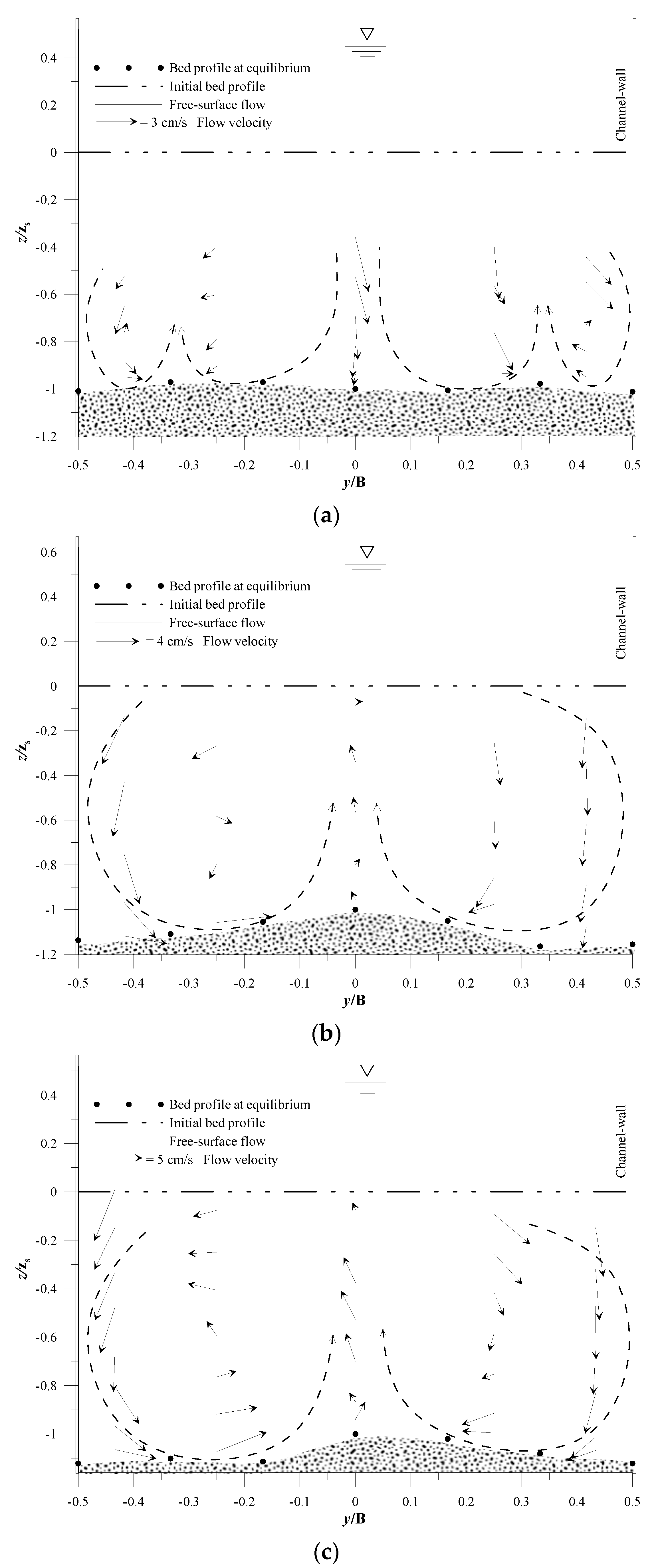
Figure 2 shows examples of the flow velocity distribution, Vyz, across the equilibrium scour hole at xs for tests T10, T12, and T13. The Vyz velocity is the resultant of the span-wise V and vertical W time-averaged velocity components. The profiles of the free surface flow (solid line), the initial bed (dash-dotted line), and the bed at the equilibrium state (bullet) are also reported in Figure 2. The rest of the sediment at the channel bottom is indicated by a random point cloud. The transversal position y is normalized by the channel width B, and the vertical position z is normalized by the maximum scour depth at equilibrium zs. In Figure 2, the coordinates y and z originate from the channel axis (y/B = 0) and the initial bed profile (dash-dotted line), respectively. The maximum scour depth zs is determined based on the longitudinal profile of the equilibrium scour at the channel axis (y/B = 0), downstream of the wooden ramp (Figure 1). The absence of velocity measurements in the upper flow region is due to the limitation of the ADV down-looking probe, being that the uppermost 7 cm of the flow could not be sampled.
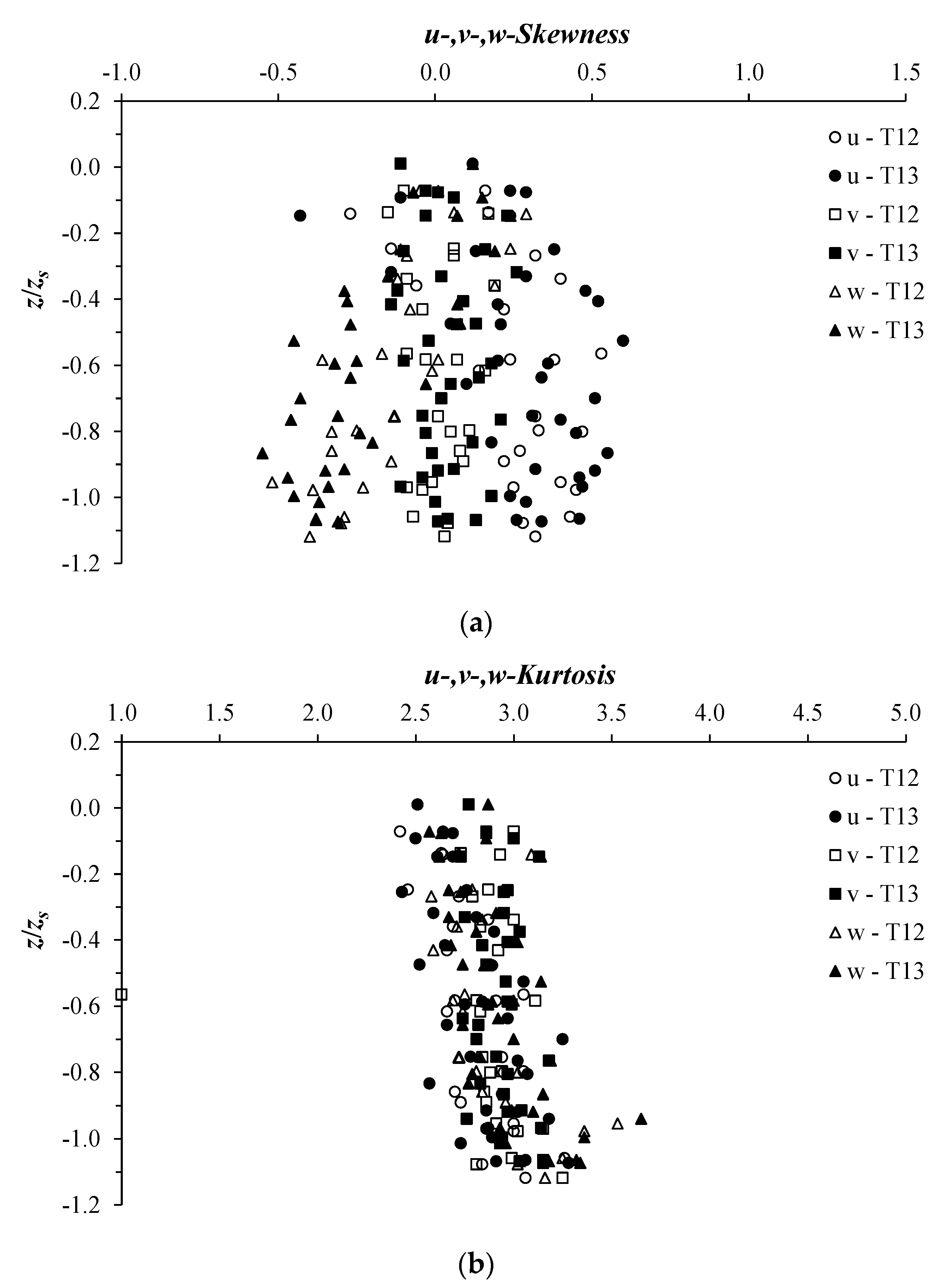
To investigate the hydrodynamic structure across the scour hole well, a high-resolution time series of the flow velocities with high quality is required. The magnitudes of the flow velocity vectors reported in Figure 2 are the result of over 4500 measurements of the instantaneous velocity components. Figure 3, as an example, shows the velocity skewness and kurtosis distribution of all measured velocities across the scour hole at xs for tests T12 and T13. Figure 3a shows that the skewness of the three velocity components u, v, and w was between −0.5 and 0.5 in most measuring positions. This implies that the measured velocity data were symmetrical. Figure 3b shows that u, v, and w kurtosis saturated to a value around 3. These results are similar to the Gaussian case (skewness = 0 and kurtosis = 3), indicating that most of the values of each measured velocity component clustered around the mean value, which means that the ADV instrument was performing satisfactorily.
In Figure 2, the flow velocity distributions in the scour cross-sections (looking downstream) clearly show the development of secondary current cells. The secondary current cells represent a circulation of fluids in the plane orthogonal to the axis of the primary flow. Figure 2 shows the formation of a helical motion rotating in opposite directions, as indicated by the curved arrow made of dashed lines in the figure. For test T10, Figure 2a shows the formation of a series of secondary current cells across the scour hole, similarly to what happens in large straight channels [20]. The four helical cells shown in the figure are symmetric with respect to the (x, z) plane at y/B = 0 (plane of flow symmetry). Figure 2a also shows an undulating sediment profile (manifested by two sediment ridges at y/B = −0.25 and 0.25) in the transverse direction. According to previous studies [20,21], the undulating sediment profile, generated by secondary current cells, may affect both the whole depth-flow field and the free surface flow pattern. Figure 2b,c indicates the formation of only two large counter-rotating vortices and a single sediment ridge, located around the channel axis (y/B = 0). For tests T12 and T13, the vortices pushed the water outward (towards the channel wall) in the upper part of the scour cross-section, while, near the bottom, the water was driven inward [19], forming the sediment ridge at the center of the channel. According to previous studies (e.g., [20,21]), the hydrodynamics of secondary currents is strongly influenced by the aspect ratio, Ar (Table 1), and the number of secondary current cells varies in proportion to the latter. This could explain the increase in the number of secondary current cells with test T10, of Ar = 2.44, compared to tests T12 and T13, of Ar = 1.76 and 1.55, respectively. Figure 2 shows that the width of the secondary current cells is 0.6hs, 0.9hs, and 0.8hs with tests T10, T12, and T13, respectively. This finding agrees with that found in previous studies [20,34], claiming that the width of secondary current cells scales with the flow depth.
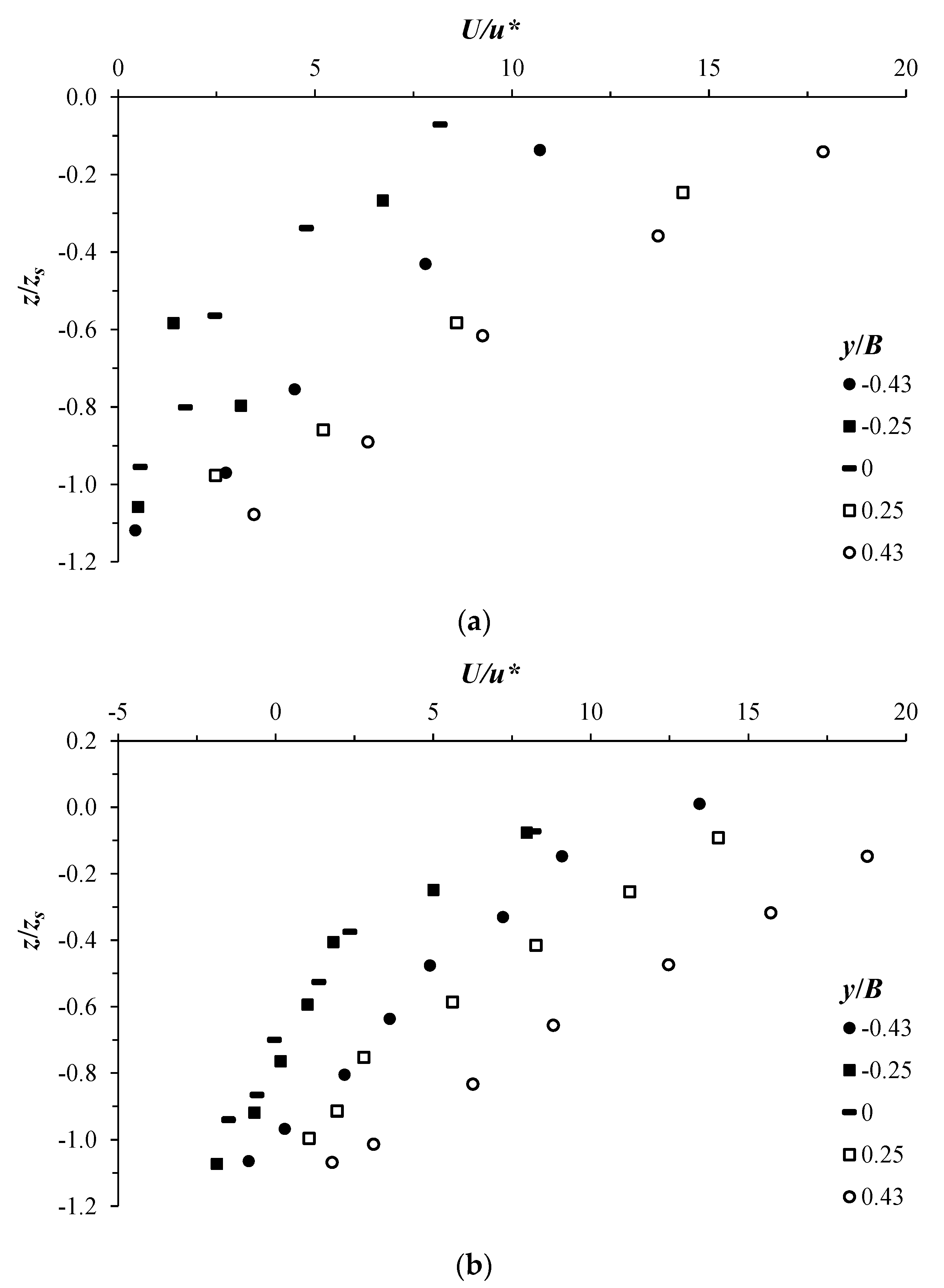
Figure 4 shows the vertical profiles of the normalized velocity U/u* at the transversal positions y/B = −0.43, −0.25, 0, 0.25, and 0.43 across the scour hole at xs. Here, the friction velocity u* was determined based on the measured primary Reynolds shear stresses U′W′ near the scour bed, and Z/hsy < 0.2, u* = (−U′W′)0.5, Z, and hsy are defined below. The vertical position z is normalized by zs, and originates at the initial bed profile, as shown in Figure 2. The data refer to test T12 (Figure 4a) and test T13 (Figure 4b). At the different transversal positions y/B, U/u* shows the same trend along the vertical. It is considerably reduced approaching the scour bed. For both tests, the profiles of U/u* are shifted from each other, indicating an anisotropic transversal distribution. At the downwelling flow regions, at y/B ≤ −0.25 and y/B ≥ 0.25 (see Figure 2), the stream-wise velocity shows the largest values, while it is reduced at the upwelling flow region, around y/B = 0. This result is in good agreement with that found by Albayrak and Lemmin [20] and Stoesser et al. [27], confirming the significant influence on the primary flow by the secondary current cells.
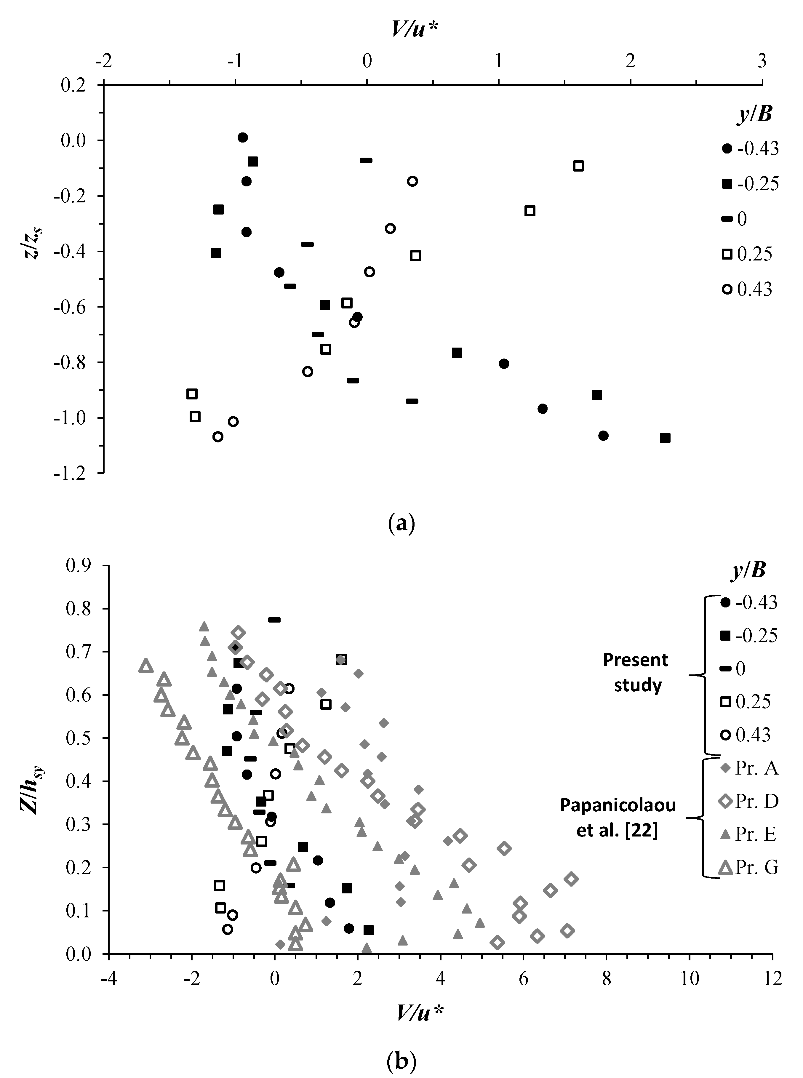
Figure 5a shows an example of the normalized span-wise velocity distribution V/u* at the transversal locations y/B = −0.43, −0.25, 0, 0.25, and 0.43, across the scour hole at xs. For the sake of brevity, due to the similar behavior of V/u* observed with the different tests, only the profiles of test T13 are included in Figure 5a. At y/B = 0, V/u* shows small values tending to zero. This is consistent with the fact that, in the plane of flow symmetry (y/B = 0), the transversal velocity component is theoretically null. Moving right or left from the plane of flow symmetry, V/u* shows considerable magnitudes. The vertical profiles clearly indicate that V/u* changes sign from negative to positive, going towards the scour bed, in the right half of the channel (y/B < 0) and vice versa in the left half, forming an x-shape with the different vertical profiles. This behavior of V/u* is a result of the development of secondary current cells across the scour hole. The x-shape of the different profiles is due to the symmetry of the vortices with respect to the (x, z) plane at y/B = 0, as shown in Figure 2c. To highlight the important role of secondary currents of the second kind in flow dynamics, a comparison of the data in the present study to field data of secondary currents of the first kind, which is usually generated in natural watercourses, is of high interest. Figure 5b shows a comparison between the vertical V/u* profiles of T13, as shown in Figure 5a, and those obtained by Papanicolaou et al. [22] on a natural river, characterized by a sequence of channel expansions and contractions along its length. It is worth mentioning that the data of Papanicolaou et al. [22] were collected along a cross-section of a natural channel of arbitrary geometry (see Figure 3 in this cited study) without GCS. Seven vertical velocity profiles were taken along the cross-section at different transversal locations A-G, using a SonTek ADV. Analysis of the vector field of the flow velocity, Vyz, in this cross-section indicates the formation of a single counterclockwise flow circulation, occupying the right half (y/B > 0) of the river (see Figure 7 in Papanicolaou et al. [22]). For the sake of comparison, in Figure 5b, the vertical position Z (capital) originates from the channel/scour bed, as in Papanicolaou et al. [22], and is normalized by hsy, the local flow depth at a given transversal position y. Applying the same procedure in normalizing the transverse direction by the width, B, of the cross-section, as in the present study, where y = 0 at the center of the cross-section, the profiles Pr. A, Pr. D, Pr. E, and Pr. G, obtained by Papanicolaou et al. [22], correspond to y/B = −0.34, 0, 0.16, and 0.40, respectively. Figure 5b shows that V/u* in the present study behaves quite similarly to that obtained by Papanicolaou et al. [22]. Moreover, the order of magnitude of V/u* within the secondary current cells for both studies seems comparable, as shown by the profiles at the counterclockwise vortices (y/B < 0 for the present study and Pr. E and Pr. G in Papanicolaou et al. [22]). The secondary current in Papanicolaou et al. [22] (of the first kind) was strongly influenced by the distortion of the primary flow, caused by an upstream bend (convex to the right riverbank) of the channel. The distortion of the primary flow underlies the formation of a single counterclockwise flow vortex, located near the right side of the channel. This could also explain the considerable increase of V/u* in the left half of the cross-section at Pr. A and Pr. D (y/B = 0), contrary to what happens in the present study conducted in a straight channel, where V/u* ≈ 0 at y/B = 0, due to the flow symmetry.
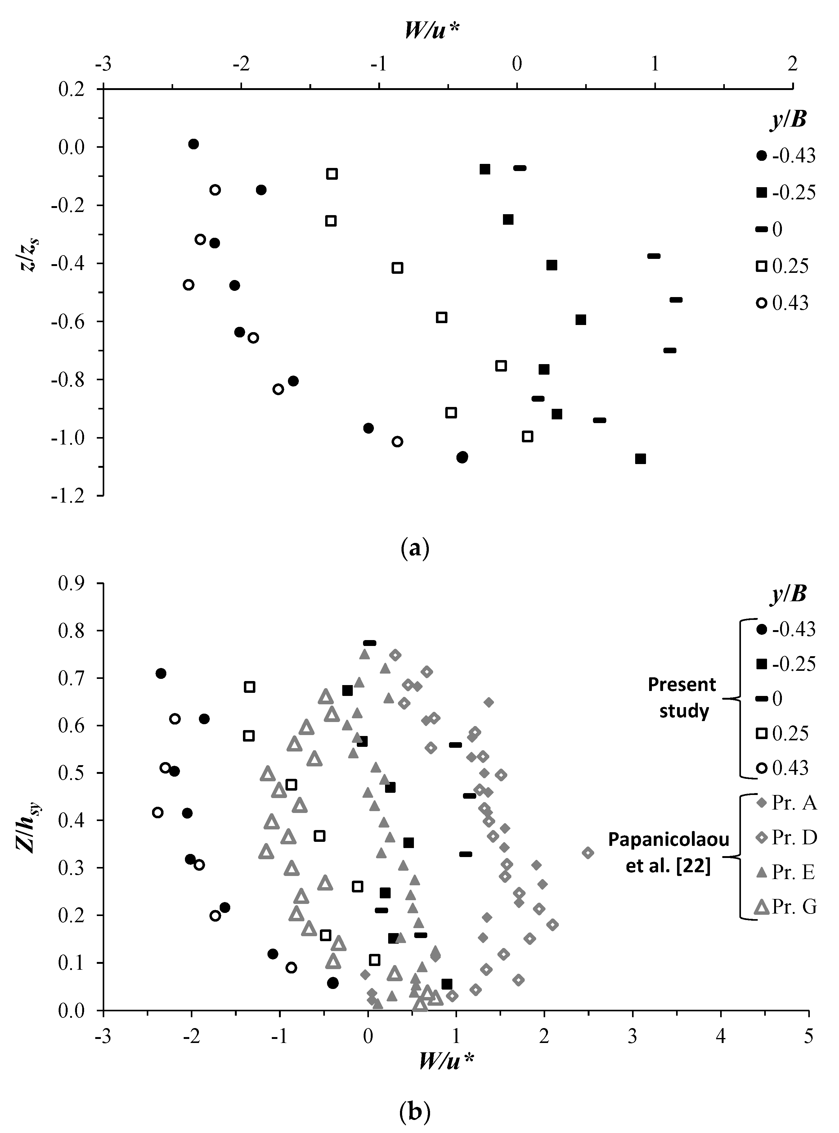
Figure 6 shows the profiles of the normalized vertical velocity W/u* for the present study and that by Papanicolaou et al. [22]. Figure 6a illustrates the profiles of W/u* of test T13 of the present study in the scour hole at the downstream position xs. To clearly show the flow features in the scour hole, we also plotted W/u* versus z/zs (as explained above). In the downwelling flow regions (y/B < −0.25 and y/B < 0.25) (see Figure 2), W/u* undergoes negative values, varying in an arched way (of concavity to the right) along the vertical: it increases in magnitude with increasing depth, reaches extreme values of O(−3) at z/zs ≈ −0.5, and then begins to gradually decrease (in magnitude), tending toward zero close to the scour bed. In the upwelling flow region (around y/B = 0), W/u* shows positive values, behaving in a similar fashion (in an arcuate way, but with concavity to the left) along the vertical as in the downwelling flow regions. In the intermediate regions (y/B = −0.25 or 0.25, as an example), W/u* can change sign from negative to positive and vice versa along the vertical. This behavior of W/u* through the scour hole is a result of the flow circulation caused by the secondary current cells. Figure 6b represents a comparison between the W/u* profiles of test T13 of the present study and those by Papanicolaou et al. [22]. Here, W/u* is plotted versus Z/hsy (as explained above). The profiles shown in Figure 6b almost indicate the same order of magnitude of W/u* for both studies, ranging between about −3 and 3. At relative transversal positions within a secondary current cell, Figure 6b also reveals that W/u* follows a similar trend along the vertical direction for both studies. The different vertical profiles of W/u* relative to a single secondary current cell show a sort of φ-shaped distribution.
4.2. Turbulence Intensities and Shear Stress Across Equilibrium Scour Hole
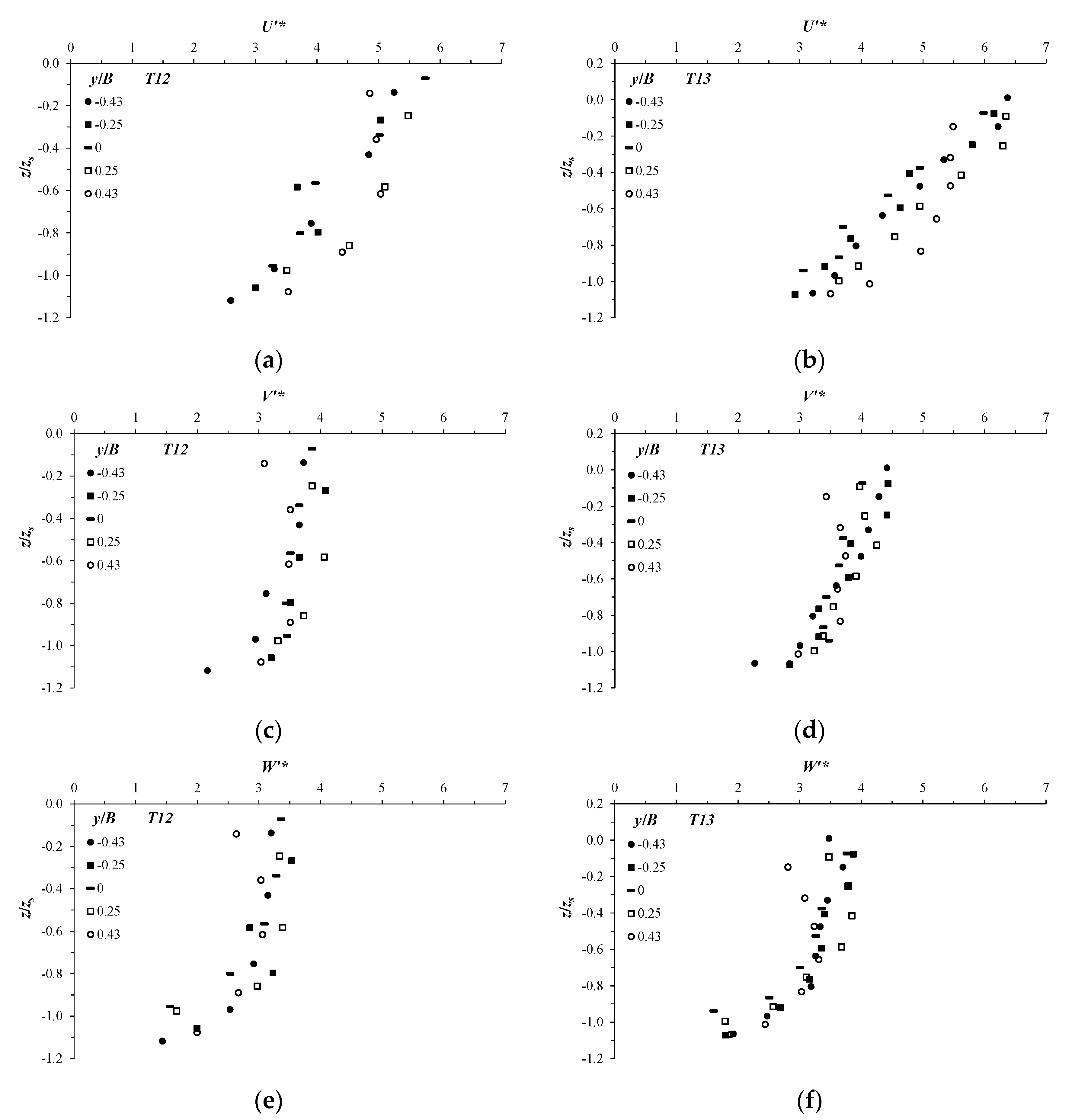
The profiles of the flow turbulence intensities at the different transversal locations y/B = −0.43, −0.25, 0, 0.25, and 0.43 across the equilibrium scour hole at the downstream position xs are shown in Figure 7. The normalized turbulence intensities in the stream wise direction, U′*, span-wise direction, V′*, and vertical direction, W′* for tests T12 and T13 are plotted in Figure 7a–f, respectively. Here, U′*, V′*, and W′* are defined as the ratio of the standard deviation of the stream-wise, span-wise, and vertical flow velocity component fluctuations in the friction velocity, u*, respectively. To show the profiles inside of the scour hole, in Figure 7, we adapt the normalized vertical coordinate z/zs (as explained in Section 4.1).
Figure 7a,b points out that the stream-wise turbulence intensity generally behaves in the same way at the different transversal locations along the water column in the scour hole. U′* decreases going down towards the scour from values of O(6) and O(7) at z/zs ≈ 0 to values of O(2) and O(3) near the scour bed in tests T12 and T13, respectively. In the upwelling flow region, U′* decreases almost linearly as z/zs decreases. In the downwelling flow region, U′* decreases in a curved way, which is more pronounced at y/B = 0.43. The profiles illustrated in Figure 7c–f also show, at first glance, a decreasing trend of V′* and W′* going to the scour bed. At z/zs ≈ 0, V′* and W′* have an order of magnitude almost half that of U′*. Contrary to what happens with U′*, V′* and W’* seem to change more gradually with the distance from the initial bed profile at z/zs = 0. Looking closely at Figure 7c–f, it can be noted that V′* and W′* change their magnitudes in an arched way along the vertical; it slightly increases starting from z/zs ≈ 0, peaks at almost z/zs = −0.5, and then begins to decrease reaching the scour bed. This is more pronounced at the downwelling flow regions, especially with W′*. The trend of variation of V′* and W′* is physically consistent with the behaviors of V/u* and W/u*, as shown in Figure 5 and Figure 6. Similar results of the flow turbulence intensity behaviors were achieved in Chang et al. [35], studying the scour process downstream of a groundsill.
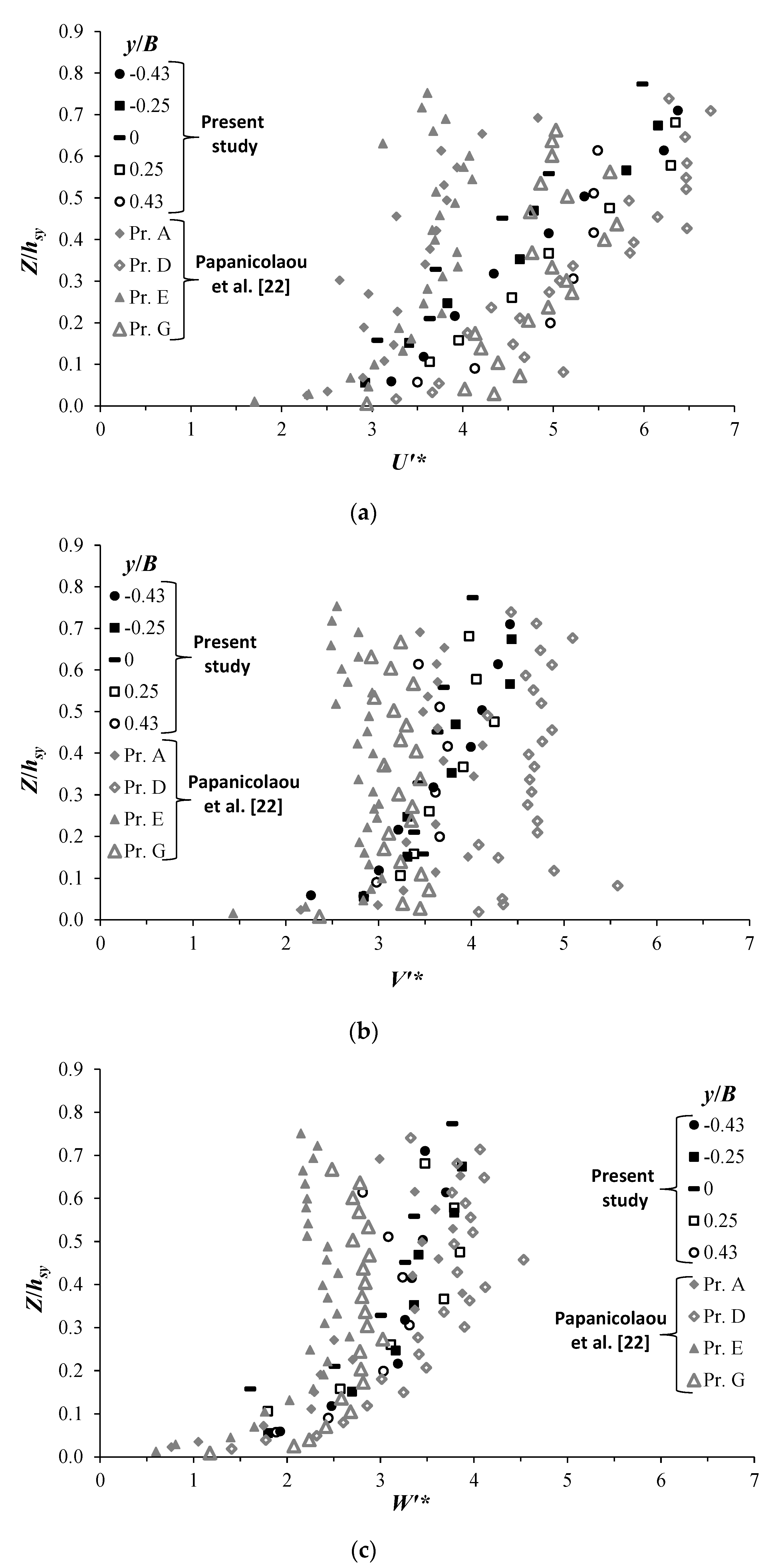
In Figure 8, we plotted the vertical profiles of U′*, V′*, and W′* of test T13, together with those conducted by Papanicolaou et al. [22]. Note that, for the sake of consistency between both studies, we adopted in these figures the normalized vertical coordinate system Z/hsy. In Figure 8, U′*, V′*, and W′* show similar trends along the water column. Furthermore, U′*, V′*, and W′* experience quite comparable values, despite the difference in hydraulic and geometric conditions among both studies. A shifting between the profiles of turbulence intensities occurred for both studies, which is pronounced with the data of Papanicolaou et al. [22], possibly due to the strong bending effect. Contrary to conventional findings in open channels, Figure 7 and Figure 8 show that the three turbulence intensities U′*, V′*, and W′* decrease as the channel bottom approaches. This means that the momentum exchange occurs from the bottom towards the surface and not the opposite, as usually confirmed by conventional findings, which may be attributed to the presence of secondary flows [22].
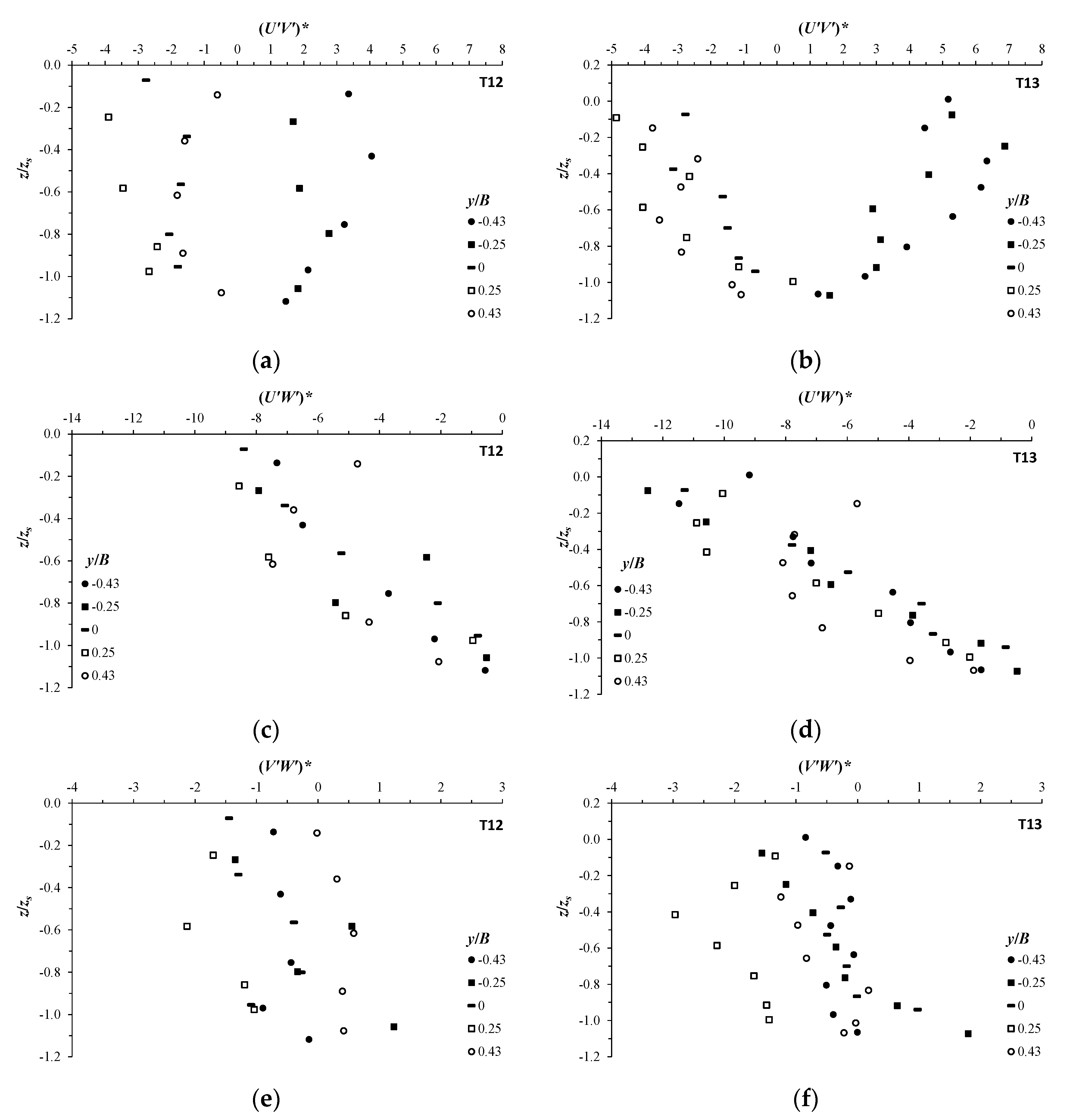
The analysis of the normalized shear stresses across the equilibrium scour hole at xs was also performed. Figure 9 reports the vertical profiles of the normalized Reynolds shear stresses at different transversal locations. The measured Reynolds shear stresses, U′iU′j (see Section 2) were normalized by the square friction velocity, u*2, and for simplicity, they are denoted as (U′iU′j)*. Figure 9a,b shows the profiles of (U′V′)* for tests T12 and T13, respectively. Figure 9c,d shows the profiles of (U′W′)* for tests T12 and T13, respectively. Figure 9e,f shows the profiles of (V′W′)* for tests T12 and T13, respectively. The shear stresses in Figure 9 indicate similar behavior to the turbulence intensities. They all show a tendency of decreasing going further towards the scour bed. Figure 9a,b shows that the span-wise shear stress (U′V′)* is of considerable magnitudes through the scour hole; it is of magnitudes almost half those of the primary shear stress (U′W′)*, shown in Figure 9c,d. The presence of positive and negative values of (U′V′)* indicates the flow symmetry with respect to the vertical (x, z) plane at y/B = 0. Theoretically, at y/B = 0, (U′V′)* must be null, which is difficult to reach experimentally. The development of secondary currents in the scour hole contributes to a significant momentum transfer in the transverse direction [27]. The secondary (cross-plane) shear stress (V′W′)*, as illustrated in Figure 9e,f, shows the smallest strengths through the scour cross-section, which are two to four times lower than those of (U′V′)* and (U′W′)*. By looking at each profile separately in Figure 9, one can note that the shear stresses show one or more peaks along the vertical, showing in general a curved profile of left or right concave distribution, which agrees well with previous studies (e.g., [20,21]). Figure 9 highlights that the three shear stress components slightly increase when comparing tests T13 with T12, which reflects a proportionality to the Reynolds number Res (Table 1). Figure 9 also points out that the shear stresses (U′V′)*, (U′W′)*, and (V′W′)* exhibit a slight increase in the downwelling flow regions compared to the upwelling regions. This behavior agrees with that observed by Albayrak and Lemmin [20] in the wall region. Albayrak and Lemmin [20] noted an opposite behavior, away from the wall region, where (U′W′)* is larger in the upwelling flow regions than that in the downwelling regions. This may imply, due to the channel’s narrowness in the present study, that the flow in the equilibrium scour hole behaves similarly to that in the wall region in straight open channels with uniform flows (without scours).
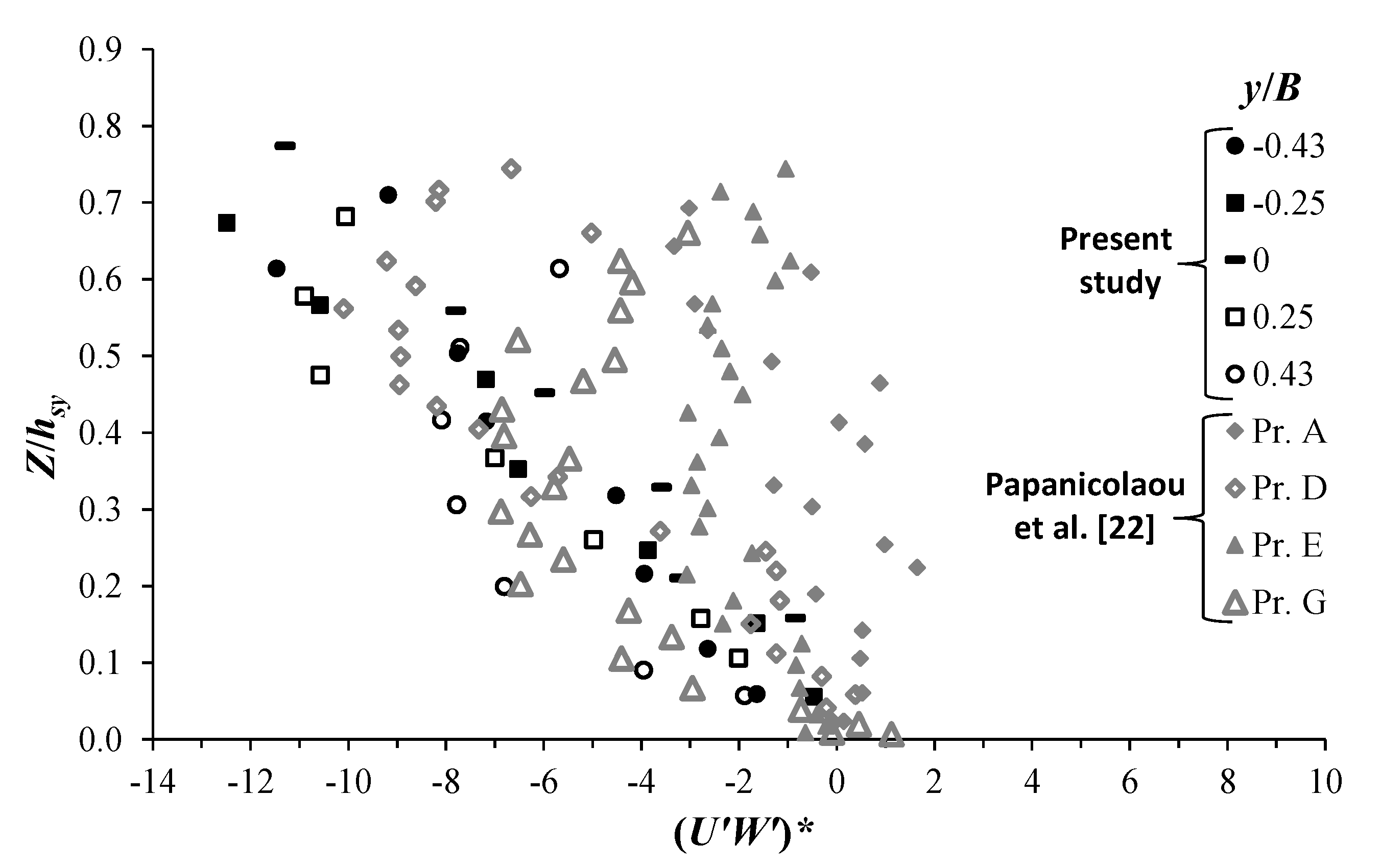
Figure 10 presents a comparison between the shear stress (U′W′)* of test T13 of the present study and that obtained by Papanicolaou et al. [22]. Here, we adopt the normalized vertical coordinate system Z/hsy (as explained above). Figure 10 indicates that, for both studies, (U′W′)* profiles have a similar tendency, especially over Z/hsy < 0.3, where the data of both studies tend to collapse together. Furthermore, at Z/hsy < 0.3, (U′W′)* in Papanicolaou et al. [22] shows the largest strengths in the downwelling regions (Pr. G) compared to that in the upwelling regions (Pr. D and Pr. E). The variation of the Reynolds shear stress values along the transverse direction, between downwelling and upwelling flow regions, reflects the oscillatory nature of the flow induced by the secondary currents, as also confirmed by Albayrak and Lemmin [20].
4.3. Contribution of Normal Stress Spatial Anisotropy to Stream-Wise Vorticity
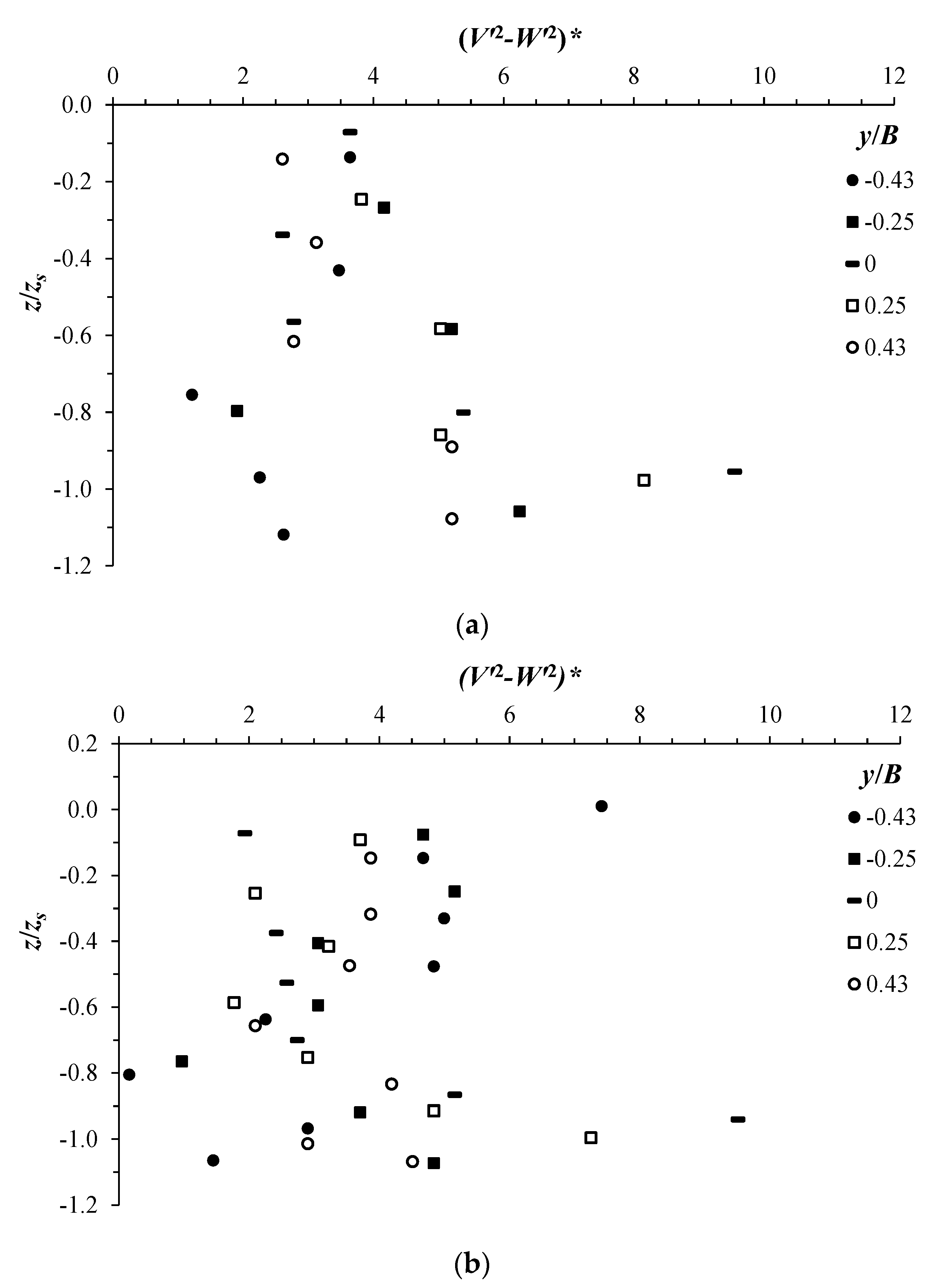
Since the generation of the second kind of secondary currents in the cross-section plane of a straight channel is induced by the inhomogeneity of the Reynolds normal and shear stresses (terms A4, A5, and A6 in Equation (4)), as cited in several previous studies (e.g., [20,26]), in Figure 11, we illustrate the vertical profiles of the anisotropy term of the normal stresses (V′2 − W′2)* at different transversal locations y/B. Here, by anisotropy, we are addressing the spatial heterogeneities of (V′2 − W′2)*. This term is normalized by the square friction velocity as: (V′2 − W′2)* = (V′2 − W′2)/u*2. It is worth mentioning that, according to the literature (e.g., [28]), the driving mechanism of stress-induced secondary flows only induces secondary currents in straight non-circular turbulent channel flows, not in laminar channel flows. Figure 11 shows considerable values of the anisotropy term of the normal stresses for both T12 and T13 tests. The profiles of (V′2 − W′2)* indicate that the latter varies considerably, both transversely and vertically. This implies the significant contribution of the term A5, as shown in Equation (4), to stream-wise vorticity generation, confirming previous findings in rough-bed, open-channel flows [27]. By treating each profile separately, it can be noted that (V′2 − W′2)* shows a maximum value near the scour mouth, and at z/zs = 0, it decreases, reaching a minimum at a vertical position of −0.8 < z/zs < −0.6, and then increases, attaining another maximum near the scour bed. This tendency is more pronounced with test T13, and is in good agreement with that shown in a previous study by Stoesser et al. [27].
For the sake of simplicity, if we neglect all gradients with respect to the stream-wise direction, i.e., ∂/∂x = 0 (which is physically valid only along a small strip dx around the downstream location of maxim equilibrium scour depth xs), the first addends in terms A1 and A3 disappear, while the term A4 vanishes completely. After some additional mathematical operations, the term A2 reduces to zero. After these assumptions, Equation (4) of the mean stream-wise vorticity for turbulent straight non-circular channel flows becomes:
The remaining terms in Equation (5) represent a balance between the convection process (term A1), the diffusion process (term A3), production process (term A5), and suppression process (term A6). The convection by secondary flow serves the transport of vorticity from production regions to the regions of diffusion by viscosity (destruction of vorticities) [28]. Previous studies [20,26] stated that the secondary current is enhanced by the production term A5 and suppressed by the term A6, which are of opposite signs, and are dominant with respect to the terms A1 and A3. Equation (5) reflects the highest importance of the production/suppression processes of vorticity, revealing the critical consideration and analysis of terms A5 and A6.
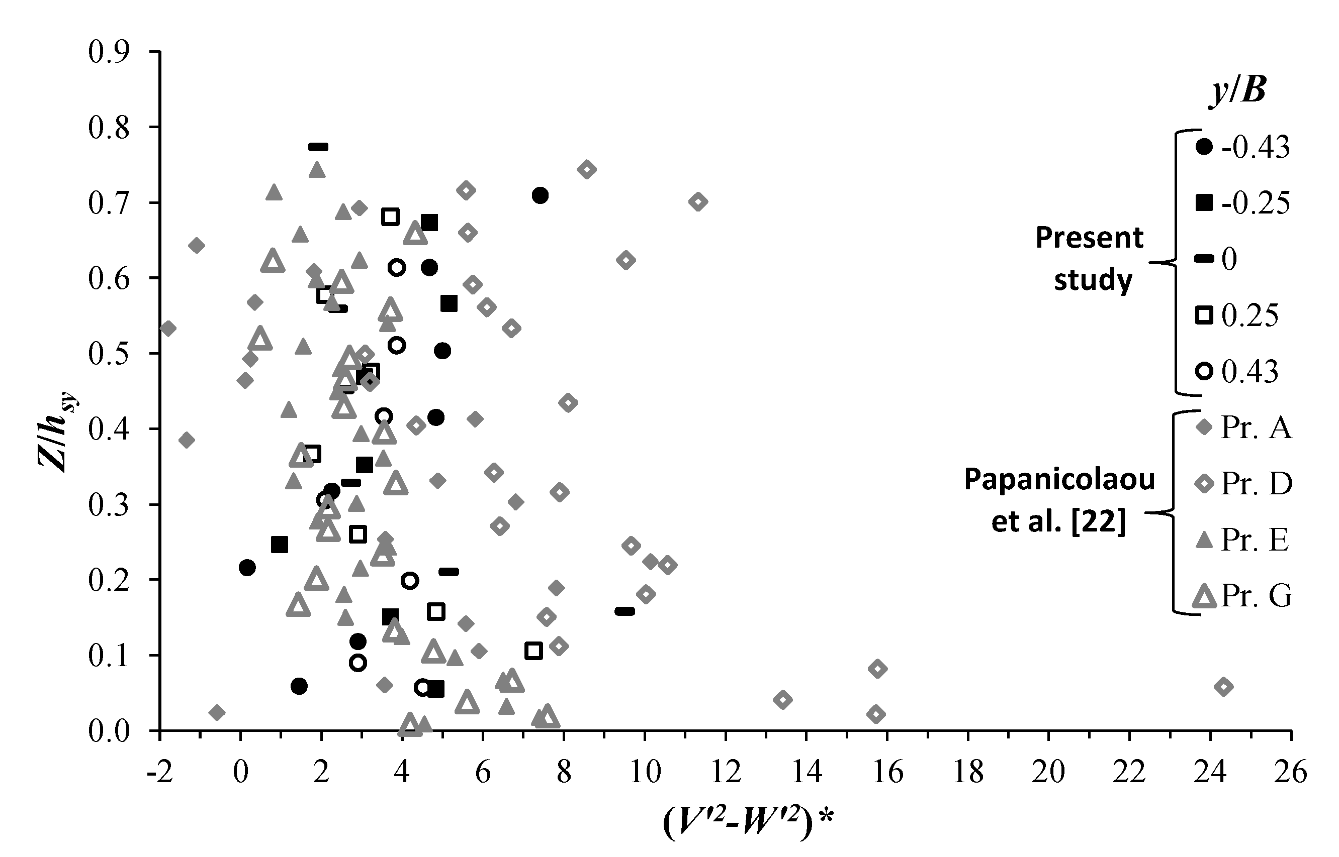
The comparison between the anisotropy term of the normal stresses (V′2 − W′2)*, shown in Figure 11, and the secondary shear stress (V′W′)*, shown in Figure 9, indicates that they have opposite signs, and (V′2 − W′2)* has an order of magnitude larger than (V′W′)*, agreeing with most of the findings in the literature. Furthermore, (V′2 − W′2)* shows greater (y, z) spatial variation compared to (V′W′)*, obviously leading to higher gradients. In the literature (e.g., [26,28,34,35,36]), the condition for the generation of a secondary current in straight non-circular turbulent channel flows was considerably discussed, giving rise to two opinion groups. The first group suggested that the anisotropy term of normal stresses, A5, is dominant, providing an essential condition to induce the secondary currents. The second group argued that this term does not play a main role in the generation of secondary currents, but that the latter are the results of the variation of bed roughness or morphology. As indicated above, Figure 11 shows maximum values of (V′2 − W′2)* near both the scour mouth and scour bed, which is more pronounced with test T13 in Figure 11b. The large values of (V′2 − W′2)* in the vicinity of the scour mouth may be the results of high turbulence intensities induced by the incoming jet flow from the grade control structure [17], while those close to the bed are perhaps enhanced by the deformation of the transversal scour bed and development of sediment ridges [1,20,22]. A significant increase of (V′2 − W′2)* near the bed channel is also clearly distinguishable with the data of Papanicolaou et al. [22], as shown in Figure 12. Figure 12 reports a comparison among the data of test T13 in the present study and those of Papanicolaou et al. [22], plotted with the normalized vertical coordinate Z/hsy. Since the secondary currents (of the first kind) in Papanicolaou et al. [22] were driven by a vortex tilting mechanism due to the channel curvature effect, the presence of high turbulence in the cross-sectional planes, generating an imbalance of normal Reynolds stresses, provides additional driving forces that maintain and enhance secondary flow motions.
5. Conclusions
Secondary current structures across an equilibrium scour hole downstream of GCSs in erodible bed channels were investigated. The measurement of the flow velocities across the equilibrium scour hole, at the downstream position of its maximum depth xs, clearly shows the formation of secondary current cells. The number of secondary current cells changes proportionally to the channel aspect ratio Ar at xs. For Ar < 2, the secondary currents across the scour hole are manifested by two large counter-rotating vortices. For Ar > 2, there has been observed a development of multi-cellular secondary currents along the scour cross-section. The secondary current structure is accompanied by the appearance of upwelling and downwelling flow regions. These flow regions are responsible for the channel bed deformation across the scour hole. The upwelling regions are characterized by a slight reduction in the primary current velocity U, giving rise to the development of sediment ridges. The downwelling regions, on the other hand, show the greatest magnitude of primary current velocity, giving the space for trough region formation across the bed scour. The alternation of several regions of upwelling and downwelling flows, in the case of a high aspect ratio, gives rise to an undulating sediment profile in the transverse direction.
The distribution of the time-averaged, span-wise, V, and vertical, W, velocity components in the cross-sectional plane of the equilibrium scour hole at the location of maximum scour depth was analyzed, confirming the development of secondary current cells of the second kind (for straight and non-circular channels). The comparison of the normalized components V/u* and W/u* with those obtained in a previous study by Papanicolaou et al. [22], for secondary currents of the first kind (driven by the curvature effect) occurred in natural channels without GCS, shows comparable orders of magnitudes for both kinds, especially for W/u*. For secondary currents of the first kind, V undergoes a slight increase, due to the considerable curvature effect, compared to that of the present study. The vertical profiles of V/u* and W/u*, taken at different transversal locations through a second current cell, indicate similar behavior of both components in the water column for both secondary kinds of currents.
The analysis of the turbulence intensities in the three flow directions across the equilibrium scour hole shows an anisotropic spatial distribution. The flow turbulence intensity in the stream-wise direction, U′*, exhibits the largest values, twice greater than those of V′* and W′*, at the mouth of the scour depth (z/zs = 0). Near the scour bed, U′*, V′*, and W′* have minimum values of O (2). In the present study, U′*, V′*, and W′* manifest similar behavior along the water column, and exhibit an order of magnitude through a secondary current cell relatively comparable to that in Papanicolaou et al. [22]. The decrease of U′*, V′*, and W′* going towards the scour bed indicates that, contrary to conventional findings, the turbulence momentum transfer occurs from the bed towards the mouth of the scour depth, at z/zs = 0.
The Reynolds shear stress distribution shows similar tendency to turbulence intensity. As compared with previous studies (e.g., [20,21,22]), the Reynolds shear stresses across the equilibrium scour hole at xs show a similar distribution to the wall layer in normal (without scours) open channel flows. This implies that the secondary currents significantly affect the flow patterns and, therefore, the morphology of the scour bed. Stronger Reynolds shear stresses were observed in the downwelling flow regions, while the weakest were found within the upwelling flow regions. The transversal undulation of the Reynolds stresses strongly influences the mass transport, and consequently the distribution of the sediment particles across the scour hole. The decrease of the Reynolds stresses going towards the scour bed indicates the flow momentum transfer from the bed towards the mouth of the scour, which may explain the generation of vertical lifting forces, giving rise to particles moving upwards.
The physical origin of the secondary currents in straight non-circular channel flows was and remains a challenging task. In the present study, we tried to understand the development of secondary current cells across the equilibrium scour hole at xs. A detailed analysis of turbulence properties was conducted. The turbulence distribution in the scour hole has shown considerable inhomogeneity. The anisotropy term of normal stresses has exhibited significant magnitudes, dominating the other terms in the mean stream-wise vorticity equation, which may reflect its potential effect in generating the secondary current motion. Furthermore, the anisotropy term of normal stresses has shown a substantial increase at the level of the scour mouth and especially near the scour bed. The interaction between the secondary currents and these boundary conditions (grade control structure and scour bed topography) may play a fundamental role in maintaining and enhancing secondary flow motion.
Author Contributions
M.B.M. performed the experiments, analyzed the data, designed the study, and wrote the paper; D.D.P., F.D.S., and M.M. contributed suggestions and discussions and reviewed the manuscript. All authors have read and agreed to the published version of the manuscript.
Funding
This research received no external funding.
Institutional Review Board Statement
Not applicable.
Informed Consent Statement
Not applicable.
Data Availability Statement
The data presented in this study are available on request from the corresponding author.
Acknowledgments
The experiments were carried out at the Hydraulic Laboratory of the Mediterranean Agronomic Institute of Bari (Italy).
Conflicts of Interest
The authors declare that they have no conflict of interest.
References
- Yang, S.-Q. Influence of sediment and secondary currents on velocity. Water Manag. 2009, 162, 299–307. [Google Scholar] [CrossRef]
- Carstens, M.R. Similarity laws for localized scour. J. Hydraul. Div. 1966, 92, 13–34. [Google Scholar]
- Bormann, N.E.; Julien, P.Y. Scour Downstream of Grade-Control Structures. J. Hydraul. Eng. 1991, 117, 579–594. [Google Scholar] [CrossRef] [Green Version]
- Balachandar, R.; Kells, J.A. Local channel in scour in uniformly graded sediments: The time-scale problem. Can. J. Civ. Eng. 1997, 24, 799–807. [Google Scholar] [CrossRef]
- Gaudio, R.; Marion, A.; Bovolin, V. Morphological effects of bed sills in degrading rivers. J. Hydraul. Res. 2000, 38, 89–96. [Google Scholar] [CrossRef]
- Lenzi, M.A.; Marion, A.; Comiti, F. Local scouring at grade-control structures in alluvial mountain rivers. Water Resour. Res. 2003, 39, 1176. [Google Scholar] [CrossRef]
- D’Agostino, V.; Ferro, V. Scour on Alluvial Bed Downstream of Grade-Control Structures. J. Hydraul. Eng. 2004, 130, 24–37. [Google Scholar] [CrossRef]
- Adduce, C.; Sciortino, G. Scour due to a horizontal turbulent jet: Numerical and experimental investigation. J. Hydraul. Res. 2006, 44, 663–673. [Google Scholar] [CrossRef]
- Meftah, M.B.; Mossa, M. Scour holes downstream of bed sills in low-gradient channels. J. Hydraul. Res. 2006, 44, 497–509. [Google Scholar] [CrossRef]
- Tregnaghi, M.; Marion, A.; Gaudio, R. Affinity and similarity of local scour holes at bed sills. Water Resour. Res. 2007, 43, W11417. [Google Scholar] [CrossRef]
- Pagliara, S.; Amidei, M.; Hager, W.H. Hydraulics of 3D Plunge Pool Scour. J. Hydraul. Eng. 2008, 134, 1275–1284. [Google Scholar] [CrossRef]
- Scurlock, S.M.; Thornton, C.I.; Abt, S.R. Equilibrium Scour Downstream of Three-Dimensional Grade-Control Structures. J. Hydraul. Eng. 2012, 138, 167–176. [Google Scholar] [CrossRef]
- Lu, J.Y.; Hong, J.-H.; Chang, K.-P.; Lu, T.-F. Evolution of scouring process downstream of grade-control structures under steady and unsteady flows. Hydrol. Process. 2013, 27, 2699–2709. [Google Scholar] [CrossRef]
- Manes, C.; Brocchini, M. Local scour around structures and the phenomenology of turbulence. J. Fluid Mech. 2015, 779, 309–324. [Google Scholar] [CrossRef]
- Papanicolaou, A.N.T.; Bressan, F.; Fox, J.; Kramer, C.; Kjos, L. Role of Structure Submergence on Scour Evolution in Gravel Bed Rivers: Application to Slope-Crested Structures. J. Hydraul. Eng. 2018, 144, 03117008. [Google Scholar] [CrossRef]
- Wang, L.; Melville, B.W.; Guan, D.; Whittaker, C.N. Local Scour at Downstream Sloped Submerged Weirs. J. Hydraul. Eng. 2018, 144, 04018044. [Google Scholar] [CrossRef]
- Ben Meftah, M.; De Serio, F.; De Padova, D.; Mossa, M. Hydrodynamic Structure with Scour Hole Downstream of Bed Sills. Water 2020, 12, 186. [Google Scholar] [CrossRef] [Green Version]
- Ben Meftah, M.; Mossa, M. New Approach to Predicting Local Scour Downstream of Grade-Control Structure. J. Hydraul. Eng. 2020, 146, 04019058. [Google Scholar] [CrossRef]
- Njenga, K.J.; Kioko, K.J.; Wanjiru, G.P. Secondary Current and Classification of River Channels. Appl. Math. 2013, 4, 70–78. [Google Scholar] [CrossRef] [Green Version]
- Albayrak, I.; Lemmin, U. Secondary Currents and Corresponding Surface Velocity Patterns in a Turbulent Open-Channel Flow over a Rough Bed. J. Hydraul. Eng. 2011, 137, 1318–1334. [Google Scholar] [CrossRef]
- Nezu, I.; Nakagawa, H. Turbulence in Open-Channel Flows; IAHR monograph series; Balkema: Rotterdam, The Netherlands, 1993. [Google Scholar]
- Papanicolaou, A.N.; Elhakeem, M.; Hilldale, R. Secondary current effects on cohesive river bank erosion. Water Resour. Res. 2007, 43, W12418. [Google Scholar] [CrossRef]
- Rhoads, B.L.; Kenworthy, S.T. Time-averaged flow structure in the central region of a stream confluence. Earth Surf. Process. Landf. 1998, 23, 171–191. [Google Scholar] [CrossRef]
- Lane, S.N.; Bradbrook, K.F.; Richards, K.S.; Biron, P.M.; Roy, A.G. Secondary circulation cells in river channel confluences: Measurement artefacts or coherent flow structures? Hydrol. Process. 2000, 14, 2047–2071. [Google Scholar] [CrossRef]
- Ianniruberto, M.; Trevethan, M.; Pinheiro, A.; Andrade, J.F.; Dantas, E.; Filizola, N.; Santos, A.; Gualtieri, C. A field study of the confluence between Negro and Solimões Rivers. Part 2: Bed morphology and stratigraphy. C. R. Geosci. 2018, 350, 43–54. [Google Scholar] [CrossRef]
- Yang, S.-Q.; Tan, S.K.; Wang, X.K. Mechanism of secondary currents in open channel flows. J. Geophys. Res. 2012, 117, 1–13. [Google Scholar] [CrossRef] [Green Version]
- Stoesser, T.; McSherry, R.; Fraga, B. Secondary Currents and Turbulence over a Non-Uniformly Roughened Open-Channel Bed. Water 2015, 7, 4896–4913. [Google Scholar] [CrossRef] [Green Version]
- Stanković, B.D.; Belošević, S.V.; Crnomarkovic, N.D.; Stojanovic, A.D.; Tomanovic, I.D.; Milicevic, A.R. Specific aspects of turbulent flow in rectangular ducts. Therm. Sci. 2016, 20 (Suppl. 6), S1–S16. [Google Scholar] [CrossRef] [Green Version]
- Meftah, M.B.; Mossa, M. Turbulence Measurement of Vertical Dense Jets in Crossflow. Water 2018, 10, 286. [Google Scholar] [CrossRef] [Green Version]
- Meftah, M.B.; Malcangio, D.; De Serio, F.; Mossa, M. Vertical dense jet in flowing current. Environ. Fluid Mech. 2018, 18, 75–96. [Google Scholar] [CrossRef]
- Meftah, M.B.; De Serio, F.; Mossa, M.; Pollio, A. Experimental study of recirculating flows generated by lateral shock waves in very large channels. Environ. Fluid Mech. 2008, 8, 215–238. [Google Scholar] [CrossRef]
- Meftah, M.B.; Mossa, M. Partially obstructed channel: Contraction ratio effect on the flow hydrodynamic structure and prediction of the transversal mean velocity profile. J. Hydrol. 2016, 542, 87–100. [Google Scholar] [CrossRef]
- Meftah, M.B.; Mossa, M. A modified log-law of flow velocity distribution in partly obstructed open channels. Environ. Fluid Mech. 2016, 16, 453–479. [Google Scholar] [CrossRef]
- Kotsovinos, N.E. Secondary currents in straight wide channels. Appl. Math. Model. 1988, 12, 22–24. [Google Scholar] [CrossRef]
- Chang, C.-K.; Lu, J.-Y.; Lu, S.-Y.; Wang, Z.-X.; Shih, D.-S. Experimental and Numerical Investigations of Turbulent Open Channel Flow over a Rough Scour Hole Downstream of a Groundsill. Water 2020, 12, 1488. [Google Scholar] [CrossRef]
- Yang, S.-Q. Mechanism for initiating secondary currents in channel flows. Can. J. Civ. Eng. 2009, 36, 1506–1516. [Google Scholar] [CrossRef] [Green Version]
Figure 1.
General sketch of the laboratory flume with the initial condition and expected scour hole (dashed profile) downstream of GCSs: B = channel width, L = distance among GCSs, q = discharge per unit width of channel, xs = position of maximum scour depth at equilibrium, zs = maximum scour depth at equilibrium, A-A = cross-section at xs. This image qualitatively indicates the transversal locations (y/B = −0.43, −0.25, 0, 0.25, 0.43) where the vertical profiles of flow velocities were measured.

Figure 2.
Vector map of the flow velocity, Vyz, across the equilibrium scour hole at xs (location of maximum scour depth downstream of the GCS): (a) test T10 of zs = 0.057 m; (b) test T12 of zs = 0.081 m; (c) test T13 of zs = 0.090 m. The random point cloud represents the remaining amount of sediment from the channel bottom at scour equilibrium.

Figure 3.
Velocity skewness and kurtosis: (a) u, v, w skewness; (b) u, v, w kurtosis.

Figure 4.
Vertical profiles of the normalized stream wise velocity U/u* at different transversal position y/B across the equilibrium scour hole at xs: (a) test T12; (b) test T13.
Figure 4.
Vertical profiles of the normalized stream wise velocity U/u* at different transversal position y/B across the equilibrium scour hole at xs: (a) test T12; (b) test T13.

Figure 5.
Normalized span-wise velocity V/u* at different transversal positions y/B across the equilibrium scour hole at xs: (a) data refer to test T13, and the vertical position z (small) originates from the initial bed profile and is normalized by zs, as in Figure 2; (b) comparison between the data of the present study of test T13 and the data obtained by Papanicolaou et al. [22] on a natural river. Here, the vertical coordinate Z (capital) originates at the scour/channel bed and is normalized by the flow depth hsy. The profiles Pr. A, Pr. D, Pr. E, and Pr. G were taken at y/B = −0.34, 0, 0.16, and 0.40, respectively.

Figure 6.
Normalized vertical velocity W/u* at different transversal positions y/B across the equilibrium scour hole at xs: (a) W/u* of test T13 plotted versus z/zs; (b) comparison between W/u* of test T13 of the present study and that of Papanicolaou et al. [22], considering the vertical coordinate system Z/hsy.

Figure 7.
Vertical profiles of the flow turbulence intensities at different transversal locations across the equilibrium scour hole at xs: (a,b) stream-wise turbulence intensity U′* for tests T12 and T13, respectively; (c,d) span-wise turbulence intensity V′* for tests T12 and T13, respectively; (e,f) vertical turbulence intensity W′* for tests T12 and T13, respectively.

Figure 8.
Comparison of the flow turbulence intensities of test T13 in the present study and those in Papanicolaou et al. [22]: (a) the stream-wise turbulence intensity U′*; (b) the span-wise turbulence intensity V’*; (c) the vertical turbulence intensity W′.
Figure 8.
Comparison of the flow turbulence intensities of test T13 in the present study and those in Papanicolaou et al. [22]: (a) the stream-wise turbulence intensity U′*; (b) the span-wise turbulence intensity V’*; (c) the vertical turbulence intensity W′.

Figure 9.
Reynolds shear stresses normalized by the square friction velocity at different transversal positions y/B across the scour hole at xs: (a,b) span-wise shear stress (U′V′)* for tests T12 and T13, respectively; (c,d) primary shear stress (U′W′)* for tests T12 and T13, respectively; (e,f) secondary shear stress (V′W′)* for tests T12 and T13, respectively.

Figure 10.
Comparison of the primary Reynolds shear stress (U′W′)* of test T13 in the present study with those in Papanicolaou et al. [22]. Here, we adopt the normalized vertical coordinate Z/hsy.
Figure 10.
Comparison of the primary Reynolds shear stress (U′W′)* of test T13 in the present study with those in Papanicolaou et al. [22]. Here, we adopt the normalized vertical coordinate Z/hsy.

Figure 11.
Vertical profiles of the normalized anisotropy term of normal stresses at different transversal locations y/B across the scour hole at xs: (a) data of test T12; (b) data of test T13.
Figure 11.
Vertical profiles of the normalized anisotropy term of normal stresses at different transversal locations y/B across the scour hole at xs: (a) data of test T12; (b) data of test T13.

Figure 12.
Comparison of the normalized anisotropy term of normal stresses of test T13 in the present study with those in Papanicolaou et al. [22]. Here, the data are plotted versus the normalized vertical coordinate Z/hsy.
Figure 12.
Comparison of the normalized anisotropy term of normal stresses of test T13 in the present study with those in Papanicolaou et al. [22]. Here, the data are plotted versus the normalized vertical coordinate Z/hsy.


Table 1.
Hydraulic parameters of the investigated tests.
| Tests | q (m2/s) | Us (m/s) | xs (m) | zs (m) | hs (m) | u* (m/s) | Ar (-) | Fds (-) | Res (-) |
|---|---|---|---|---|---|---|---|---|---|
| T10 | 0.027 | 0.227 | 0.54 | 0.057 | 0.123 | 0.022 | 2.44 | 0.20 | 14,270 |
| T12 | 0.040 | 0.233 | 0.70 | 0.081 | 0.171 | 0.024 | 1.76 | 0.17 | 18,577 |
| T13 | 0.046 | 0.236 | 0.73 | 0.090 | 0.194 | 0.025 | 1.55 | 0.18 | 20,466 |
Publisher’s Note: MDPI stays neutral with regard to jurisdictional claims in published maps and institutional affiliations. |
© 2021 by the authors. Licensee MDPI, Basel, Switzerland. This article is an open access article distributed under the terms and conditions of the Creative Commons Attribution (CC BY) license (http://creativecommons.org/licenses/by/4.0/).
Share and Cite
MDPI and ACS Style
Ben Meftah, M.; De Padova, D.; De Serio, F.; Mossa, M. Secondary Currents with Scour Hole at Grade Control Structures. Water 2021, 13, 319. https://doi.org/10.3390/w13030319
AMA Style
Ben Meftah M, De Padova D, De Serio F, Mossa M. Secondary Currents with Scour Hole at Grade Control Structures. Water. 2021; 13(3):319. https://doi.org/10.3390/w13030319
Chicago/Turabian StyleBen Meftah, Mouldi, Diana De Padova, Francesca De Serio, and Michele Mossa. 2021. "Secondary Currents with Scour Hole at Grade Control Structures" Water 13, no. 3: 319. https://doi.org/10.3390/w13030319
Note that from the first issue of 2016, this journal uses article numbers instead of page numbers. See further details here.