Use of the Hydraulic Model for the Operational Analysis of the Water Supply Network: A Case Study

Abstract

This paper presents an analysis of the operation of the water supply system. The analysed network provides water to six small towns. The water supply network covers rural areas of approximately 50 square kilometres with a total of 6130 inhabitants (2020). The area is characterised by relatively large differences in elevation. The water-pipe network supplies water mostly to family housing, public utility buildings, recreational buildings, service and craft entities, religious buildings, and commercial facilities and farms, including breeding farms. The network is supplied from one deep water well and a centrally located water supply tank. A hydraulic model was used for the analysis. The model was developed using the Epanet program, based on numerical and operational data. After validation, selected measurement points were used to calibrate the model. Furthermore, a series of simulations were performed to illustrate the network operation for variable water supply and demand conditions. Single-period analysis was used for modelling due to the type of data obtained. The model allowed for the determination of the head of pressure in the network points and flows in particular sections for the operation parameters studied. The analysis showed that at present, the network is not operating stably. In the case of average demand, water is supplied to all users, but there are areas in the network characterised by high pressure. On the other hand, during maximum water demand, due to the limited water supply to the water reservoir, from which most of the network is supplied, there are water deficiencies that cannot be compensated for by the operating pumping system.

1. Introduction

The water supply network is an essential and very expensive part of the entire water supply system. It is designed to supply water of the appropriate quality, at the quantity, pressure, and time required by consumers. For the network to operate properly, it must be well designed and constructed, and used effectively. Furthermore, the operation and control of a water supply system have a key effect on the costs associated with water distribution, and thus on its final price. A hydraulic model is a versatile tool that can be used both at the stage of designing a new network and during the operation of an already existing network. The use of information technology and available software offers virtually unlimited possibilities to solve problems related to water distribution that would not be possible with conventional methods (e.g., the possibility to simulate the quality of water supplied in the network). The computer simulation of network operation facilitates the making of important decisions concerning current operations in a water supply company [1,2,3,4].

The numerical analysis of the network helps to evaluate the network from an operational perspective. It is particularly useful for the optimisation of the operation of already existing networks. Modelling is helpful, for example, when planning the flushing of individual sections of the water supply system, or shutting them down for repair and maintenance purposes. Furthermore, an analysis of the behaviour of the network during the maximum water demand makes it possible to find locations causing problems in network operation and to test the designed solutions. Simulation of the occurrence of failures on the main pipes makes it possible to check that the balance of the system and the water supply to consumers is not disturbed. The model can then be used to test alternative solutions to prevent the consequences of failures. It can help to evaluate the cost of a water network based on local landscape characteristics and the available renewable water resources. A great interest and increasingly common use of numerical methods for the computation of water-pipe networks is being observed [5,6,7,8,9,10,11,12,13,14].

The use of hydraulic models in the operation of water supply systems requires verification and calibration. This process allows for an appropriate level of correspondence between the actual values measured on the site and the calculation results. Only a properly calibrated model allows for the reproduction of actual operating conditions in a water supply system [15,16].

Aim and Scope of the Study

The aim of the study was to analyse the operation of the water supply system that supplies water to six localities in Poland. The analysis was based on a hydraulic model. The model allowed for the examination of network operation at present and the identification of the places in the network that pose problems with its use.

The scope of the study included the following:

• Obtaining information about water demand and the parameters of the water supply network;
• Preparing and inputting the data into the model;
• Model verification;
• Model calibration based on pressure measurements for selected fire hydrants;
• Conducting a series of simulations of network operation for variable supply and demand conditions and analysis of the results.

2. Description of the Existing State

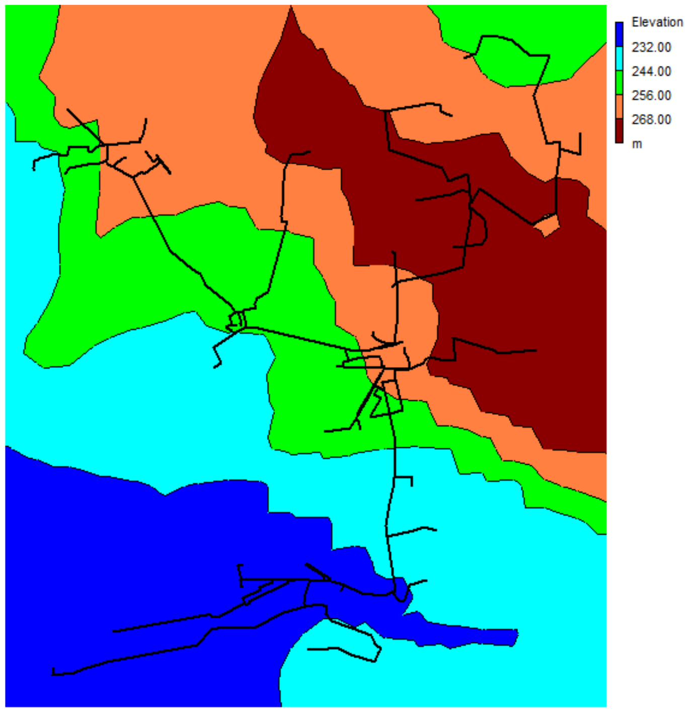
The analysed water supply area is located in the north-western part of the Silesian Voivodeship. In the west, the area borders on the Opole Voivodeship. The water supply network provides water to six localities, each with a population of about 230 to 1500 people. The analysed area is characterised by a relatively large variation in altitude. The layout of the contour lines is presented in Figure 1.

The difference between the lowest and highest points is 55.1 m. The water intake is located in an area with an altitude of 228 m a.s.l. The water tank is located in an area with an altitude of 265.8 m a.s.l., while the altitude of the highest point that receives water from the water tank is 277.1 m a.s.l. The terrain profile is therefore unfavourable for the operation of the water supply system.

The analysed water supply area supplies water to rural areas with distributed land development, mainly with residential single-family buildings. There are also public utility buildings, service and craft businesses, religious buildings, commercial facilities, and farms, including livestock farms (poultry and cattle breeding). Part of the area is covered by recreational buildings. None of the buildings are higher than three storeys. The buildings are partly connected to the sanitary sewage system or are equipped with holding tanks and on-site sewage treatment plants. Hot water is prepared locally for domestic purposes.

Over the last few years (2014–2019), the number of inhabitants in individual localities remained mostly constant. Only a very small decrease was observed, with the maximum change for one of the localities being −6% over six years. In 2019, there were 6131 people living in the area covered by the network.

The water supply network supplies water to an area of about 50 km². Water is supplied from one water intake, located in the northern part of the area. Water is pumped into the network directly from the drilled well through the technological system located at the water treatment station. The pumping system is equipped with a frequency converter that maintains pressure at a level of ca. 51 mH₂O. The maximum efficiency of the pumping system is ca. 33 m³/h. It is impossible to measure the daily or hourly volumes of water pumped into the network. Water from the intake is supplied directly to consumers living in two localities and, using a Ø160 mm transit pipe, to the water tank, located in the central part of the network. The total tank capacity is 150 m³, whereas its active capacity is ca. 100 m³. Next, the water from the tank is pumped by means of a pumping system into the water supply network supplying the four other localities. The pumping system maintains a pressure level from 32 to 42 mH₂O. The average capacity of the pumping station is 13–20 m³/h, and, in the period of the largest water demand, the maximum capacity is 45 m³/h.

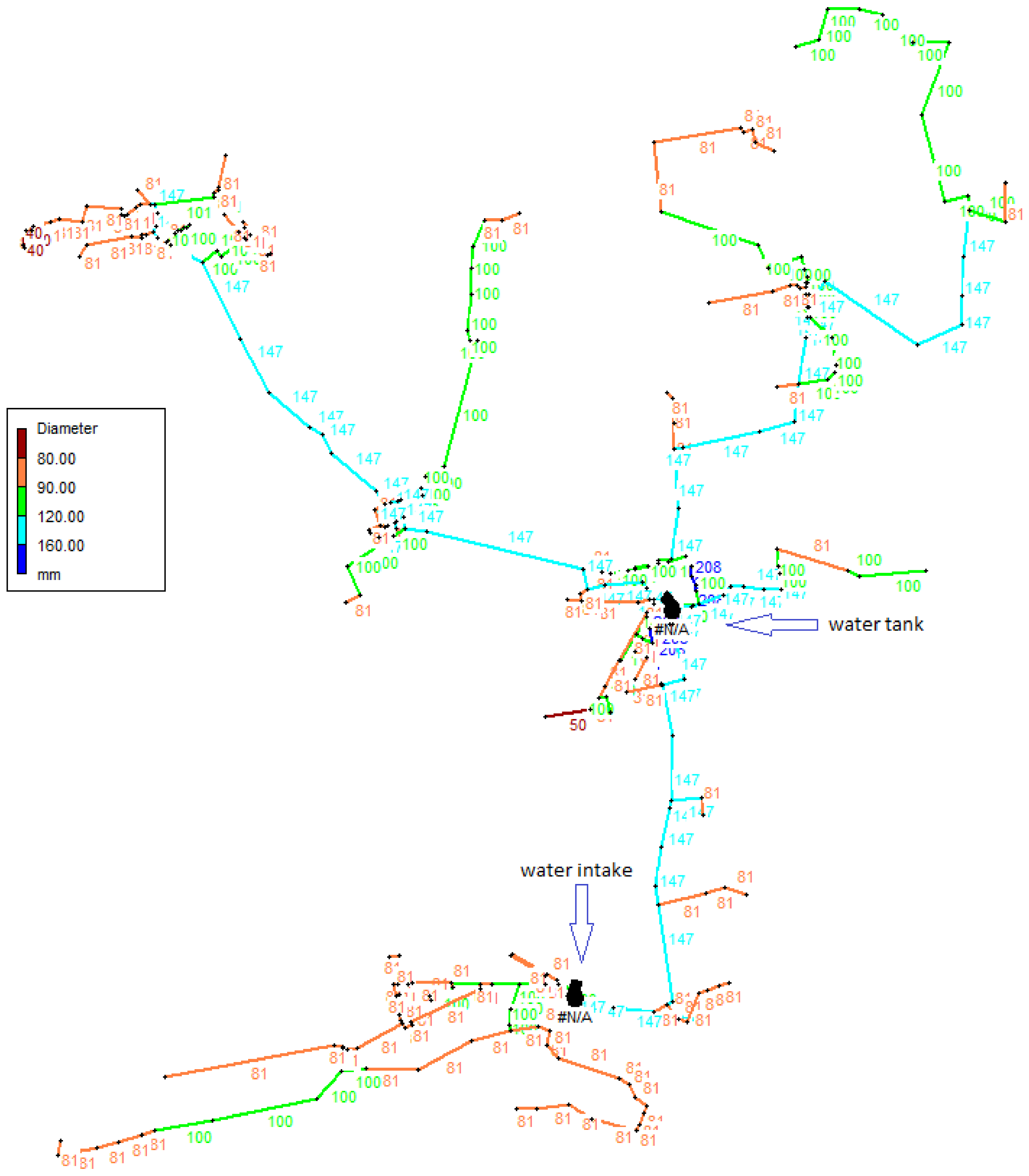
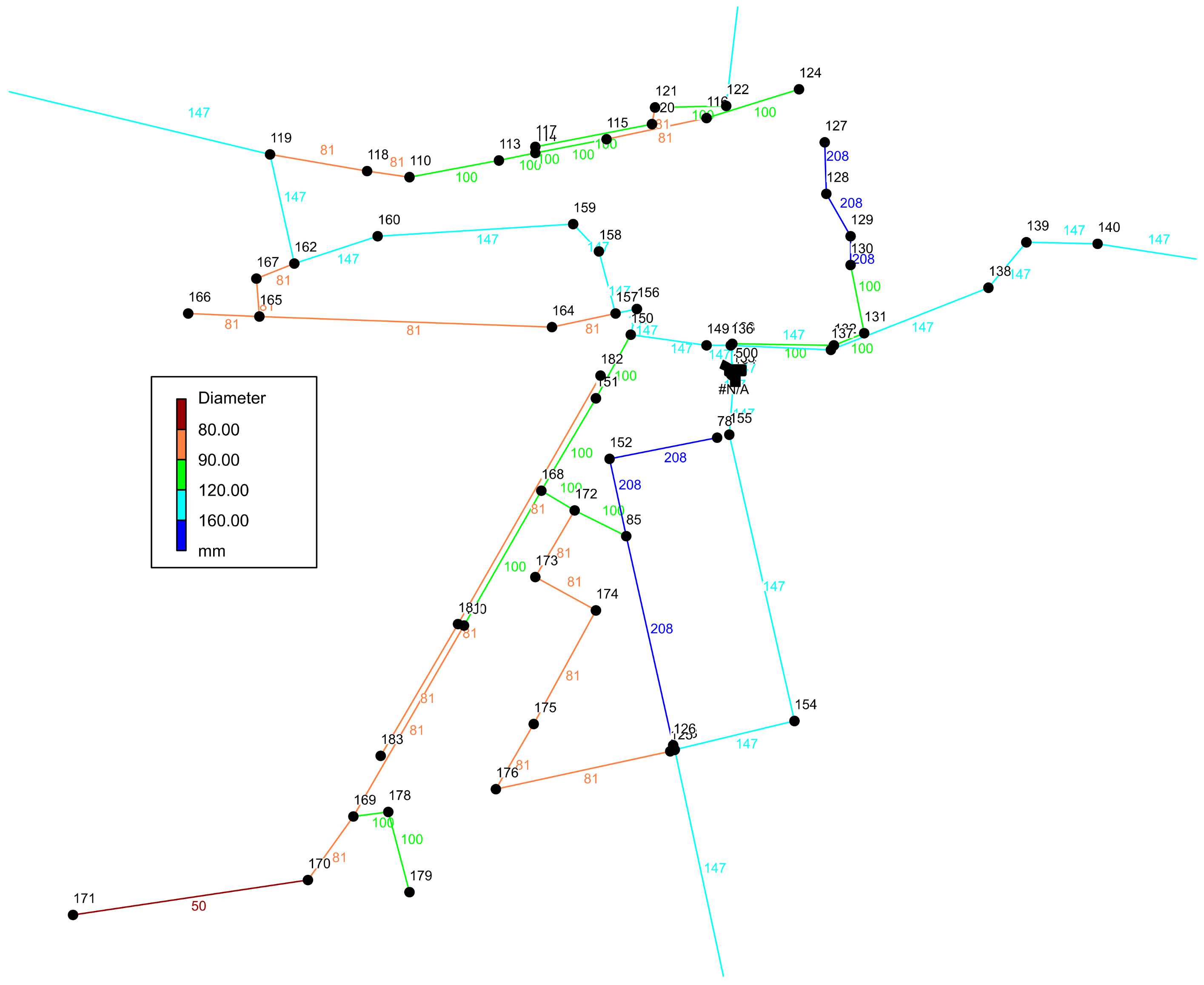
The total length of the network in the analysed area is ca. 58.1 km. The network is made of PVC pipes with diameters of DN 225, DN 160, DN 110, and DN 90. The network lengths for individual diameters are as follows: DN 225—ca. 860 m, DN 160—ca. 17,100 m, DN 110—ca. 16,900 m, and DN 90—ca. 23,230 m.

Pipe diameters for the whole network are shown in Figure 2. Due to the model specificity, internal diameters are shown in the drawing (internal diameters were used for calculation). The main transit pipes connecting the individual localities have a diameter of Ø160 mm (internal Ø147 mm).

The data from average sales in 2019 obtained from the network operator were used to determine the water demand in the model. Using these data, the average daily water demand in the analysed area was calculated, taking into account the specificity of individual customers. For the entire network, average daily water demand was 412 m³/d. This value takes into account the losses occurring in the network, estimated by the operator at a level of ca. 15%.

Two large users (a poultry farm and a cattle farm) are located on the transit route between the water intake and the tank. The calculated daily average demand for these consumers was as follows:

• Poultry farm—47.2 m³/d;
• Cattle farm—12.9 m³/d.

During the analysis of the operation of the water supply system, it is important to determine water consumption variability. Changes in this respect occur both during the day and over the year. Two coefficients should be used to evaluate the changes: Ndmax (maximum daily variability) and Nhmax (maximum hourly variability). Due to the impossibility of measuring the variability of water flow for both locations of water supply in the analysed network (pumping stations in the water intake and the field tank), the values of the coefficients of water demand variability were estimated based on the information obtained from the operator and the related literature. The size of the area where water should be supplied and the type of development were taken into account. It was also assumed that the network efficiency for the maximum water demand in summer is insufficient. Consequently, higher coefficients than those resulting from the observed maximum flows were used. In the summer period, the highest water production was 755 m³/d.

Therefore, the following values were adopted:

• Daily variability coefficient Ndmax = 2;
• Hourly variability coefficient Nhmax = 3.

The maximum hourly water demand (Qhmax) calculated using the above coefficients was 103 m³/h.

All water consumers in the area covered by the network are equipped with water meter sets. The number of water supply connections at the end of 2019 was 1075. Unit water demand for domestic purposes (only households) ranged, depending on the locality, from 30 to 81 dm³/user·d. Furthermore, taking into account all other needs (farms and other users), the unit water demand ranged from 44 to 171 dm³/user·d. The highest average water consumption was observed in the area where the tank is located—171 dm³/user·d. This is due to the large quantities of water used in agriculture.

3. Hydraulic Model

Modelling is about reproducing, as much as possible, the course of a real process. In the case of water supply networks, the modelling process allows for the mapping of water behaviour in pipes, taking into account such parameters as water demand distribution, pressure and its losses, and flow rates. It is essentially impossible to perform measurements of these parameters for the entire network, due to both costs and time consumption. The development and calibration of a model is more efficient and allows for the simulation of network operation. Furthermore, the network inventory analysis conducted during modelling facilitates checking the correctness of input data describing the network. Modelling is particularly important when converting or expanding an existing network. It allows for the quick analysis of different variants of the proposed solutions and the choice of the most advantageous one. The effects of increasing the load of the already existing system can be estimated, and errors that arise during the design of new sections can be detected.

The present study discusses a hydraulic model developed using Epanet 2 software. This software was created to simulate water distribution systems by the United States Environmental Protection Agency in 1994 [17]. The software is free, but many commercial applications for mathematical simulations of hydraulics use Epanet algorithms. The gradient algorithm-hybrid nodal-loop iterative method was used to simplify the cumbersome Cross calculation procedure. A one-period analysis was employed to model the network due to the scope of the obtained operational data. The Hazen–Williams formula was chosen to calculate the pressure loss in the pipes, which is used to calculate the turbulent water flow.

The developed network model consists of 314 nodes connected by 315 pipe sections. The model includes one water source, one water tank, and pumping systems. The developed model is characterised by a high degree of detail.

3.1. Input Data for the Model

The development of the network design was based on the available general map, from which terrain ordinates, pipe layout, and network diameters were read. Other data on the water supply network, such as materials and the method of supplying water to the two zones, were obtained from the network operator. Multipoint curves based on the operating ranges given by the operator were used as pump performance profiles. The total volume of the water supply tank was assumed to be 150 m³, whereas the active volume of the tank was 100 m³. The range of diameters for pipes used in the model was DN 90–225 mm. The model took into account the internal pipe diameters. The pipe material was PVC.

The water demand levels were assigned to each node based on the estimated average water demand (it is impossible to input linear water demand in the model). The pipe roughness coefficient for PVC was determined based on the data from pipe manufacturers.

3.2. Model Calibration

The model was calibrated based on the measurement points in locations of fire hydrants installed in the network. Due to the level of detail in the model, the required number of points should be at least 2% of the nodes. The calibration file used data for 85 points, which is 27% of the nodes. Pressure measurements performed during the inspection of fire hydrants in 2019 were used for calibration. Due to the impossibility of determining the actual flow values in the networks during the review, water demand was assumed to be at an average daily level.

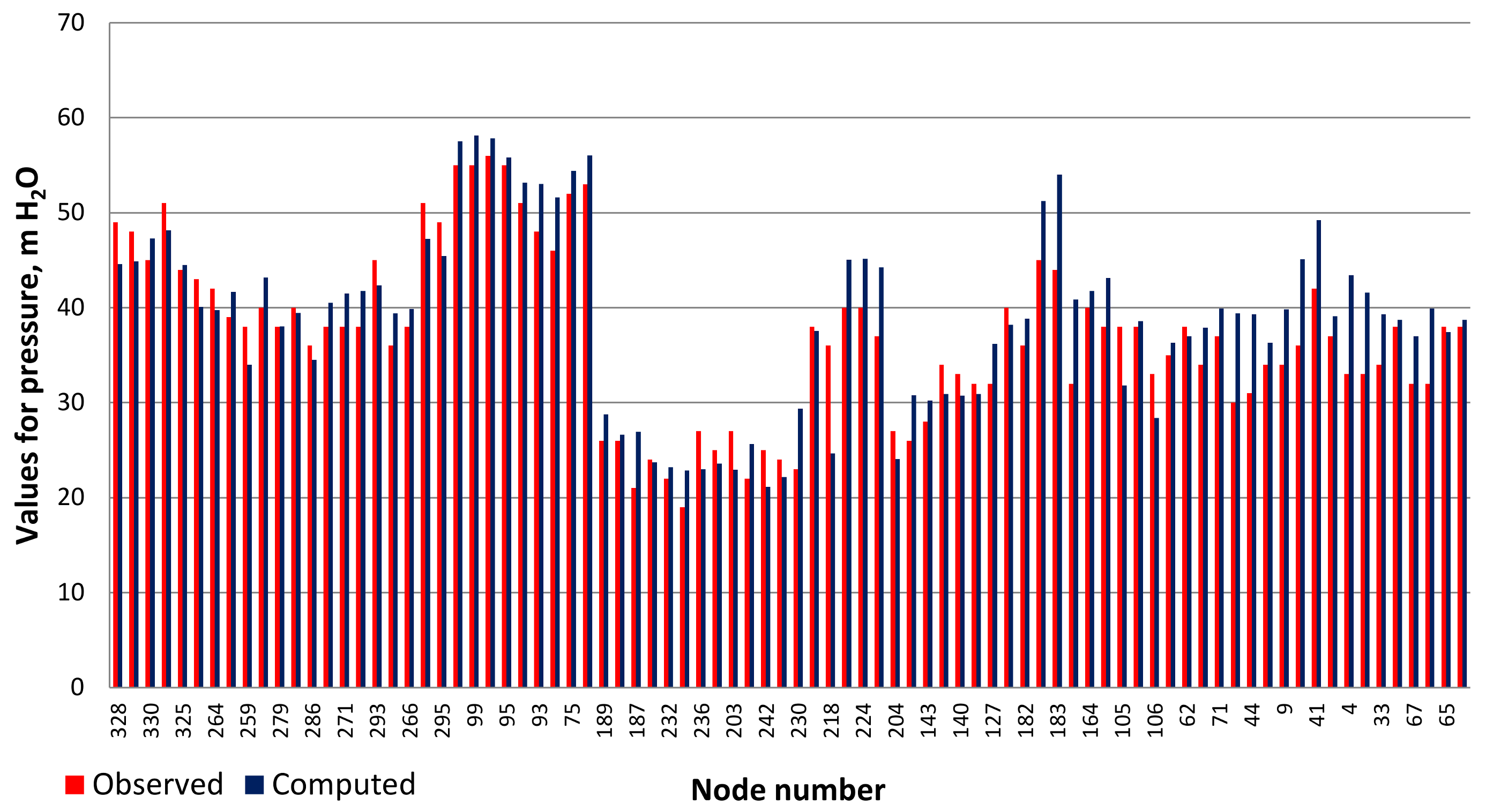
During the simulation of network operation, the pressure values in the nodes were calculated and then compared with the pressures measured at the nodes. This comparison was used to evaluate an average absolute error between all pairs of pressure values, which was 4.5 mH₂O. The mean square error was 3.7 mH₂O. This shows a good representation of the real conditions that prevail in the simulated network. Only in a few nodes was the difference between the observed and simulated value near or slightly above 10 mH₂O (4 nodes) or 7 mH₂O (7 nodes). This may be due to the measurements being carried out in different conditions of water demand than assumed, which is unfortunately difficult to verify, due to the lack of measurement capabilities of the network.

The calculated correlation coefficient between the mean value observed and the simulated pressure was 0.895. Therefore, the correlation can be considered as good. It was adopted, based on the calibration, that the developed model was correct and represented a reliable representation of the tested water supply network. Figure 3 presents a comparison of pressures for the nodes studied.

4. Analysis of Network Operation

Using a calibrated model of the water supply network, several simulations showing its operation for variable water supply and demand conditions were performed. The following network operation variants were analysed:

• conditions of standard water demand for the current supply system;
• conditions of maximum water demand for the current supply system;
• network operating conditions at an increased capacity of the water supply tank and pumping system efficiency.

The optimal range of pressures for the water supply network was set from 20 mH₂O to 55 mH₂O. Pressure below 20 mH₂O is unacceptable in Poland due to fire safety reasons. High pressures may increase the risk of network failure—the upper limit of the acceptable pressure for main and distribution pipes in Poland is 60 mH₂O.

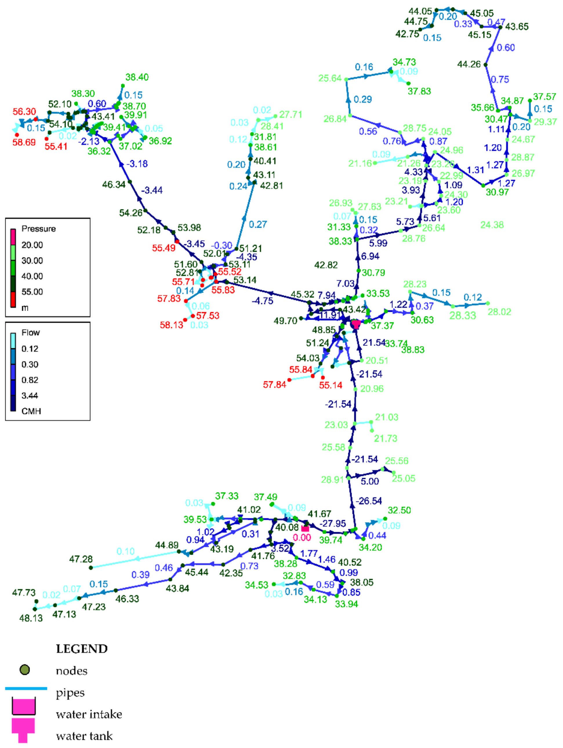
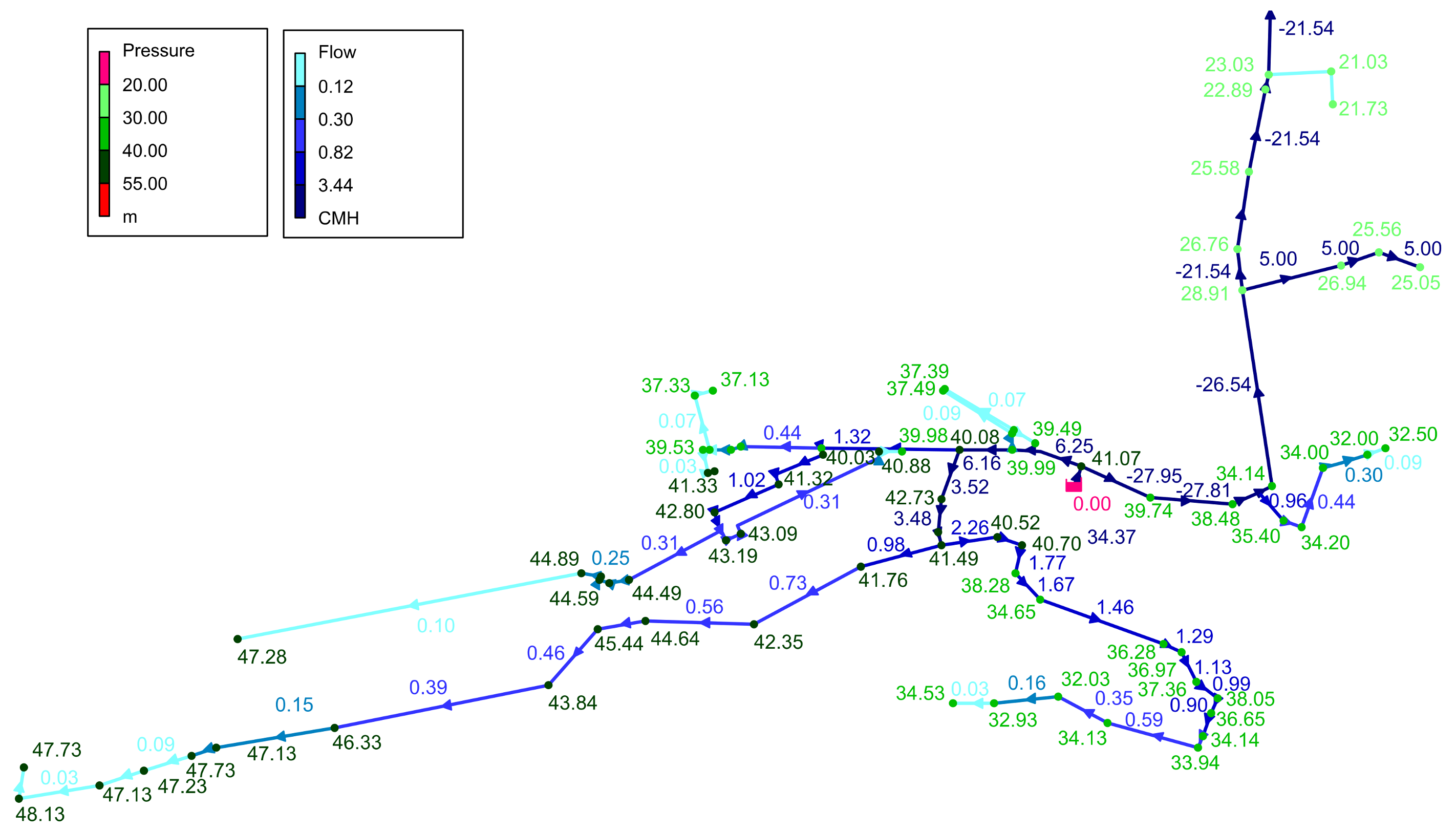
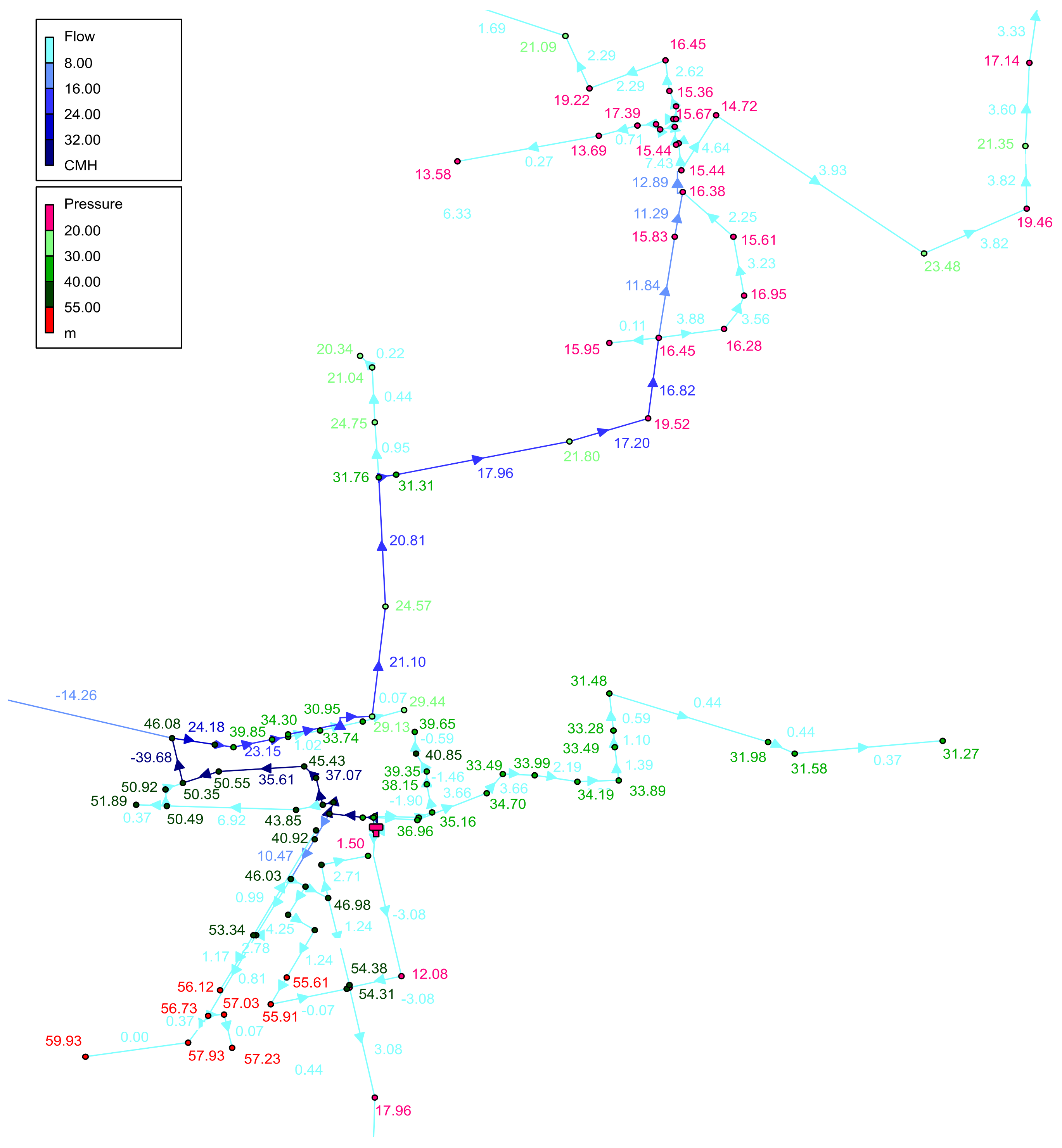
In the first analysed variant of network operation, a simulation was carried out for the water demand characteristic of average hourly water demand. Figure 4 shows simulated pressure values in individual nodes and water flow for the entire network. Due to the lower legibility of the figure for individual localities, Figure 5, Figure 6 and Figure 7 show different parts of the analysed area. The values of individual parameters are presented using a variable colour scheme for nodes and pipes. The numerical values at the nodes refer to pressure (in mH₂O). A red colour was used to show excessively high pressure values (above 55 mH₂O), and a pink colour to show excessively low values (below 20 mH₂O). A green colour was used for the other values, with the colour saturation increasing with increasing value. The numerical values in the middle of the pipes refer to flow (in m³/h). A blue colour was used to show the flow value, with the colour saturation increasing with increasing value. The arrows indicate the direction of water flow in the pipes.

Figure 4 shows that the height of available pressure in individual nodes ranges substantially from ca. 21 mH₂O in the north-eastern part of the network to a maximum of ca. 59 mH₂O in the north-western part.

In the area with water supplied directly from the water intake, the pressure ranged from 32 mH₂O to a maximum of ca. 50 mH₂O (Figure 5). Flow rates were characteristic of average water demand. For this reason, part of the water pumped into the network flows into the existing tank, where it is collected and then used during increased demand (the analysis was started with a minimum level of water in the tank).

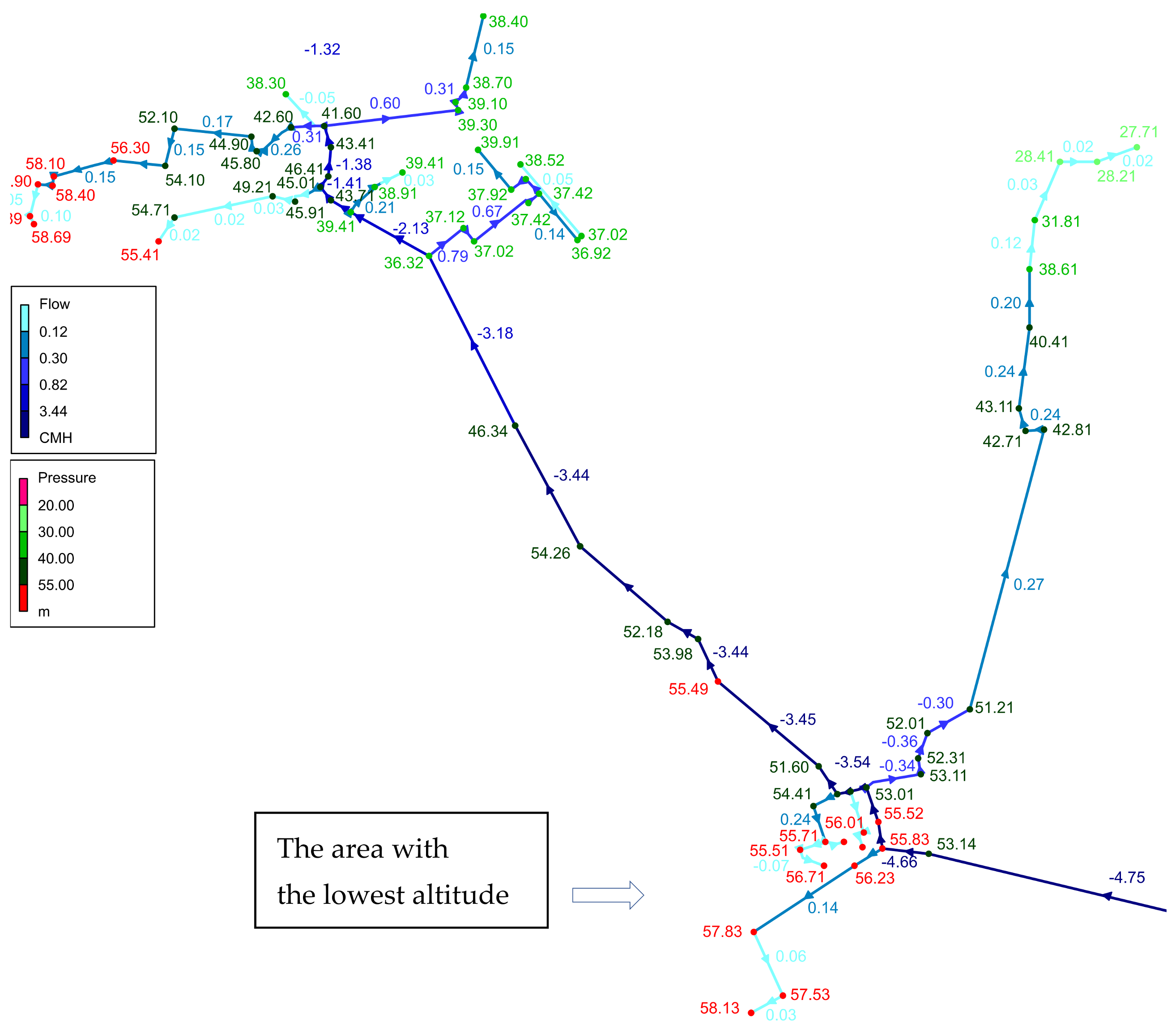
Figure 6 shows the area covering the north-western part of the network. High pressure values were observed for the locality at the lowest altitude: they ranged from ca. 51 to 58 mH₂O. This is caused by the terrain profile and the need to maintain an adequate pressure reserve for the operation of the network under conditions of increased water demand. Due to the long transit distance to the next locality, the flow losses are also much higher at higher water demands. The altitude of the locality (Figure 1) is also unfavourable for the network’s operation. At the end of the network branch in the eastern direction, the values do not exceed 28 mH₂O. In the northernmost locality, the pressure is more varied, ranging from about 38 mH₂O in the eastern part of the locality to almost 59 mH₂O in the western part.

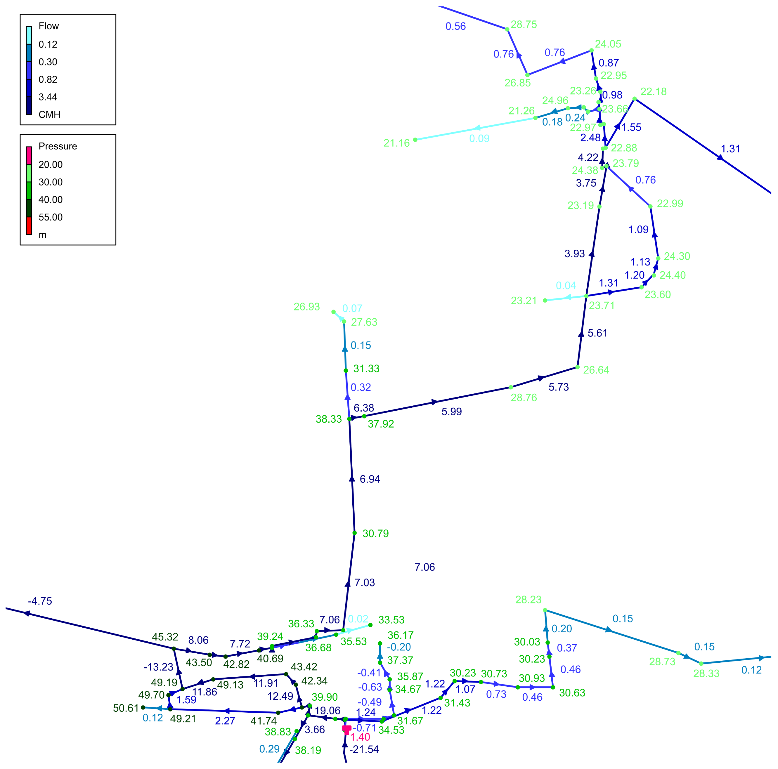
Figure 7 shows the central area of the network, including the water tank. It can be observed that while the water supply from the tank is maintained at the required pressure level (from about 28 to about 50 mH₂O), it only slightly exceeds 20 mH₂O in further sections of the network.

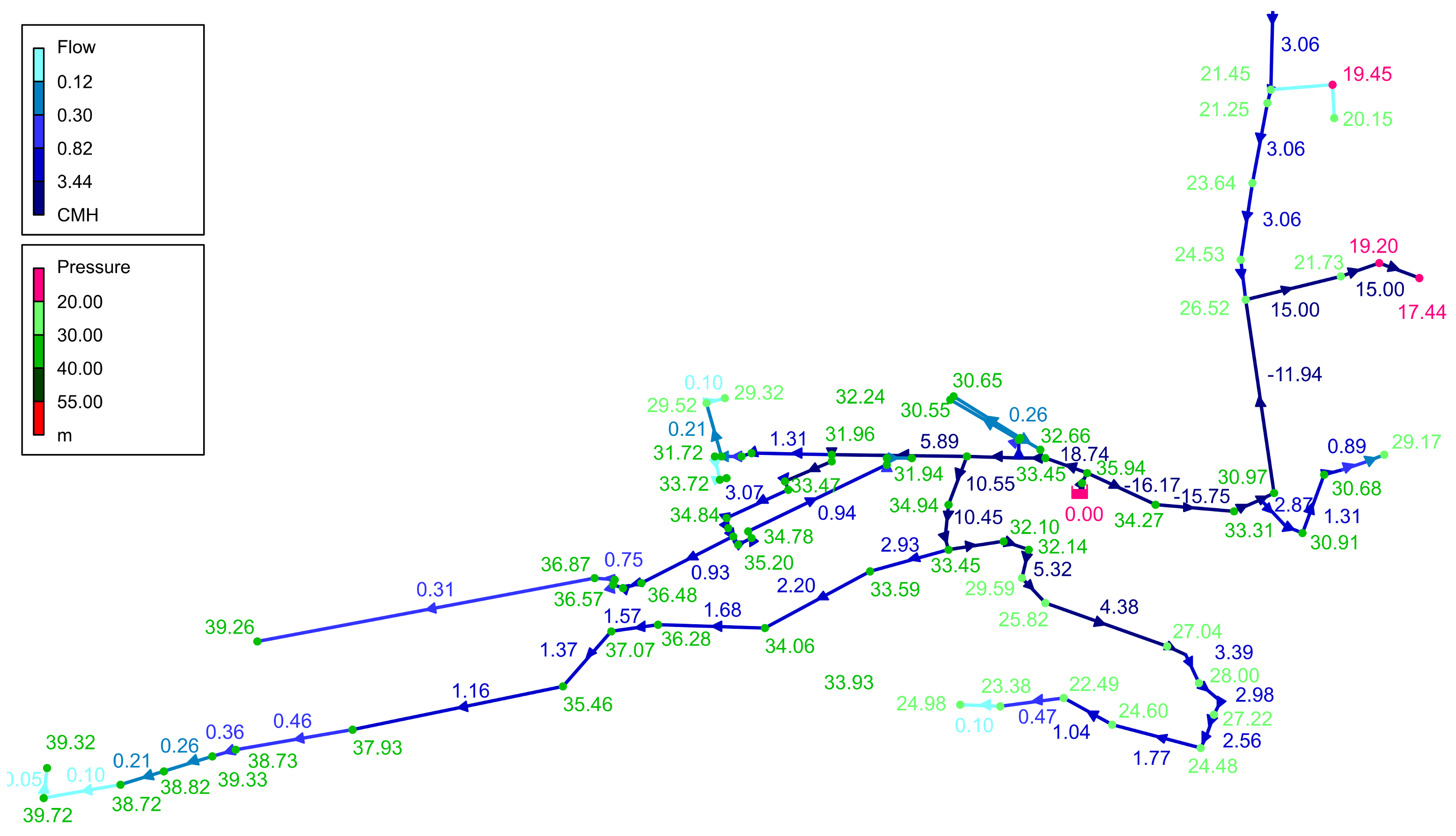
The second analysed variant of network operation takes into account the maximum hourly demands (variant B). Unfortunately, with such a network load, the program reports an error message. The network cannot be balanced during the calculation. Although the pumping systems at the water intake and the tank reach their maximum efficiency, they cannot supply the required volumes of water and ensure the correct pressure in the network. For this reason, it is impossible to present pressure values for the entire network. The figure below shows the area supplied directly from the water intake in the southern part of the network (Figure 8).

A decrease in the available pressure is observed compared to the previous simulation (Figure 5). The pressure in main pipes ranges from ca. 21 mH₂O to a maximum of ca. 40 mH₂O, with the pressure reduced by ca. 10 mH₂O. There are greater decreases in the water supply connections, where the pressure is below 20 mH₂O. In the case of water flow, a change of flow direction can be observed for the transit pipe between the intake and the tank. Water from the tank flows towards large users (poultry and cattle farms). Since the analysis was started with an average level of water in the tank, the tank was gradually emptied. Based on the simulation, it can be concluded that in the case of maximum demand, the water supply system does not operate stably, and its capacity is insufficient, even if the available tank capacity is taken into account.

Figure 9 shows pipe diameters in the central locality. In the main part, ensuring transit to the next locality, from node 110 to node 122, the pipe diameter is 110 mm and is insufficient, especially for maximum flows. The section between nodes 118, 119, and 110, which is made of PVC 90, should also be remodelled.

The third analysed variant of network operation took into account increased tank capacity and the efficiency of the pumping system connected to it. A water supply tank with a capacity twice as large as the current one (200 m³) was adopted. The pumping system efficiency was increased to ca. 65 m³/h at a pumping height of 52 mH₂O. Since water supply problems occurred at maximum water demands during previous simulations, they were also taken into account in this variant of the analysis. If these water supply parameters are accepted, the simulation runs correctly, and the program does not report an error message. However, in this case, high values of available pressure were found in previously observed areas of the network with a shortage in other network nodes (a decrease below 20 mH₂O). Figure 10 shows simulated pressure values in individual nodes and water flow for this part of the network, where the biggest problems with water supply occurred. The same colour scheme was used to present the values of individual parameters as before.

5. Conclusions

The model was developed and calibrated to test different variants of network operation and the effects of each of them. Simulation results were obtained from the analysis and used to draw the following conclusions:

• Currently, the network is not operating steadily. For the average demand, water is supplied to all consumers, but there are high-pressure areas of the network, reaching almost 60 mH₂O. Furthermore, during the hours of maximum water demand, due to the limited water supply to the tank, which is used for a major part of the network, there are water shortages which cannot be compensated for by the pumping system. The biggest problems with water supply occur in the eastern part of the network.
• The currently operated water supply tank has an active capacity that is insufficient for the demands in the network. In order to improve network reliability, it is necessary to increase the capacity of the existing water tank or build a new one. The estimated operating capacity of both tanks, due to the size of the network and large demand variability, should be ca. 50% of the average daily water demand. The active capacity of the current tank is less than 25% of this value, and therefore it does not ensure the required volume of water. The total tank capacity should also take into account water volume for firefighting purposes, which, with the current number of inhabitants, should be 50 m³.
• In order to improve network operation, the pipelines ensuring water transit between localities should be redesigned, especially in the locality in the central part. Currently, they have diameters that are too small (DN 90 and DN110) and cause relatively large pressure losses at maximum flow rates.
• In order to improve the operating conditions, it is necessary to install measuring devices in the existing network supply points (water intake and tank) to enable continuous reading and recording of water pressure and flow values. This will allow for the evaluation of the actual variability and enable the correct choice of a new volume of the water tank and network management. It would also be advantageous to install measurement devices in selected network nodes, in transit pipes connected to individual localities. After the modernization of the network and the installation of appropriate measuring devices, the obtained results will be implemented in the model in order to better adjust to real conditions.
• In the future, diameters for transit water supply networks should be increased, especially between the current water intake and the existing tank, and between the central locality and the area with the lowest operating pressure. Due to long distances and maximum flow rates, transit pipelines should have an internal diameter of 200 mm (e.g., PVC 225 pipes). The change of diameters can be introduced gradually (e.g., networks can be rebuilt during repairs of individual streets or replaced in case of increased failure rates). Due to the extent of such projects, it should be planned in the long term.

In a longer perspective, the model will be used to analyse the effect of new water intakes on network operation, with the evaluation of the required capacity and possible location.

References

- Gosiewska, E. Dobrze “zaprogramowana” firma. Wodociągi-Kanalizacja 2004, 1, 13–16. (In Polish) [Google Scholar]
- Sroczan, E.; Urbaniak, A. Narzędzia informatyczne dla systemów wodociągowo-kanalizacyjnych. Wodociągi-Kanalizacja 2004, 1, 17. (In Polish) [Google Scholar]
- Kwietniewski, M. Monitorowanie i Geograficzne Systemy Informacji w procesie współczesnej eksploatacji systemów dystrybucji wody i odprowadzania ścieków. Gaz Woda i Technika Sanitarna 2005, 4, 9–14. (In Polish) [Google Scholar]
- Kara, S.; Karadireka, I.E.; Muhammetoglua, A.; Muhammetoglu, H. Hydraulic modeling of a water distribution network in a tourism area with highly varying characteristics. Procedia Eng. 2016, 162, 521–529. [Google Scholar] [CrossRef] [Green Version]
- Bałut, A.; Urbaniak, A. Kryteria wyboru informatycznych narzędzi modelowania sieci wodociągowych. Gaz Woda i Technika Sanitarna 2009, 6, 11–15. (In Polish) [Google Scholar]
- Willet, J.; King, J.; Wester, K.; Dykstra, J.E.; Essink, G.H.P.; Rijnaarts, H.H.M. Water supply network model for sustainable industrial resource use a case study of Zeeuws-Vlaanderen in the Netherlands. Water Resour. Ind. 2020, 24, 100131. [Google Scholar] [CrossRef]
- Xu, Y.; Zhang, X. Research on pressure optimization effect of high level water tank by drinking water network hydraulic model. Procedia Eng. 2012, 31, 958–966. [Google Scholar] [CrossRef] [Green Version]
- Klawczyńska, A. Modelowanie układów rozprowadzania wody. Wodociągi-Kanalizacja 2006, 9, 30–31. (In Polish) [Google Scholar]
- Rutkowski, T. Od modelowania, przez symulację do sterowania. Wodociągi-Kanalizacja 2005, 10, 12–15. (In Polish) [Google Scholar]
- Zimoch, I. Zastosowanie modelowania komputerowego do wspomagania procesu eksploatacji systemu wodociągowego. Ochrona środowiska 2008, 3, 31–35. (In Polish) [Google Scholar]
- Haifeng, J.; Wei, W.; Kunlun, X. Hydraulic model for multi-sources reclaimed water pipe network based on Epanet and its applications in Beijing, China. Front. Environ. Sci. Eng. China 2008, 2, 57–62. [Google Scholar]
- Kotowski, A.; Pawlak, A.; Wójtowicz, P. Modelowanie miejskiego systemu zaopatrzenia w wodę na przykładzie osiedla mieszkaniowego Baranówka w Rzeszowie. Ochrona środowiska 2010, 2, 43–48. (In Polish) [Google Scholar]
- Zhang, Q.; Zheng, F.; Jia, Y.; Savic, D.; Kapelan, Z. Real-time foul sewer hydraulic modelling driven by water consumption data from water distribution systems. Water Res. 2021, 188, 116544. [Google Scholar] [CrossRef] [PubMed]
- Ociepa, A.; Lach, J. Nowoczesne techniki w eksploatacji sieci wodociągowej i kanalizacyjnej. Ecol. Chem. Eng. 2007, 14, 567–574. (In Polish) [Google Scholar]
- Ateş, S. Hydraulic modelling of control devices in loop equations of water distribution networks. Flow Meas. Instrum. 2017, 53, 243–260. [Google Scholar] [CrossRef]
- Bałut, A.; Urbaniak, A. Weryfikacja i walidacja jako niezbędne etapy tworzenia modelu symulacyjnego sieci wodociągowym. Gaz Woda i Technika Sanitarna 2012, 4, 160–164. (In Polish) [Google Scholar]
- Rossman, L.A. Epanet 2 Users Manual; U.S. Environmental Protection Agency: Cincinati, OH, USA, 2000.
Figure 1.
Altitude profile of the analysed area.
Figure 2.
Water supply network plan with pipe diameters, and the location of the water intake and water tank.
Figure 3.
Comparison of the pressure parameter for the nodes: computed and observed.
Figure 4.
The pressure and flow rate in the network for average hourly water demand (the entire network)—all customers have guaranteed water supply.
Figure 5.
The pressure and flow rate for the average hourly water demand; zoomed view of the map on the southern part of the network together with the intake.
Figure 6.
The pressure and flow rate for the average hourly water demand; zoomed view of the map on the north-western part of the network.
Figure 7.
The pressure and flow rate for the average hourly water demand; zoomed view of the map on the central part of the network.
Figure 8.
Pressure head reduction for the maximal hourly water demand; zoomed view of the map on the southern part of the network.
Figure 9.
The diameters for the central part of the network, near the water tank.
Figure 10.
The pressure and flow rate for maximum hourly water demand - change of tank capacity and pump efficiency ensures water supply to all users.
Publisher’s Note: MDPI stays neutral with regard to jurisdictional claims in published maps and institutional affiliations. |
© 2021 by the author. Licensee MDPI, Basel, Switzerland. This article is an open access article distributed under the terms and conditions of the Creative Commons Attribution (CC BY) license (http://creativecommons.org/licenses/by/4.0/).
Share and Cite
MDPI and ACS Style
Kepa, U. Use of the Hydraulic Model for the Operational Analysis of the Water Supply Network: A Case Study. Water 2021, 13, 326. https://doi.org/10.3390/w13030326
AMA Style
Kepa U. Use of the Hydraulic Model for the Operational Analysis of the Water Supply Network: A Case Study. Water. 2021; 13(3):326. https://doi.org/10.3390/w13030326
Chicago/Turabian StyleKepa, Urszula. 2021. "Use of the Hydraulic Model for the Operational Analysis of the Water Supply Network: A Case Study" Water 13, no. 3: 326. https://doi.org/10.3390/w13030326
Note that from the first issue of 2016, this journal uses article numbers instead of page numbers. See further details here.