
Uncertainty Analysis of SWAT Modeling in the Lancang River Basin Using Four Different Algorithms
by
 , ,
, ,
Xiongpeng Tang
1,2,3, 
Jianyun Zhang
2,3,
Guoqing Wang
2,3,*,
Junliang Jin
2,3,
Cuishan Liu
2,3,
Yanli Liu
2,3,
Ruimin He
2,3 and
Zhenxin Bao
2,3 1
College of Hydrology and Water Resources, Hohai University, Nanjing 210098, China
2
Nanjing Hydraulic Research Institute, Nanjing 210029, China
3
Research Center for Climate Change, Nanjing 210029, China
*
Author to whom correspondence should be addressed.
Water 2021, 13(3), 341; https://doi.org/10.3390/w13030341
Submission received: 29 December 2020
/
Revised: 19 January 2021
/
Accepted: 26 January 2021
/
Published: 29 January 2021
(This article belongs to the Special Issue Hydrological Modeling in Water Cycle Processes)
Abstract
:The hydrological model is the primary tool for regional water resources management, allocation, and prediction. However, these models always suffer from large uncertainties from multiple sources. Therefore, it is necessary to conduct an uncertainty analysis before performing hydrological simulation. Sequential Uncertainty Fitting (SUFI-2), Parameter Solution (ParaSol), Generalized Likelihood Uncertainty Estimation (GLUE), and Particle Swarm Optimization (PSO) integrated with the SWAT-CUP software were used to calibrate the Soil and Water Assessment Tool (SWAT) model and quantify the parameter sensitivity and prediction uncertainty of the SWAT in the Lancang River (LR) Basin, which is located in the southwest of China. This model was calibrated and validated using the four algorithms both at the daily scale, and the optimal simulation results derived by the four methods showed that the SWAT model performed well over the Yunjinghong station with Nash–Sutcliffe efficiency coefficient (NSE) and coefficient of determination (R2) values greater than 0.8 both in the calibration (1975 to 1989) and validation (1990 to 2004) periods. Among the four algorithms, the ParaSol algorithm produced the best simulation result at the daily scale with NSE values of 0.89 and 0.90 for the calibration and validation periods, respectively. Furthermore, the ParaSol algorithm has the greatest proportion of simulations (94%) with an NSE greater than 0.5. Parameter sensitivity analysis results demonstrated that the four methods all can be used for parameter sensitivity analysis in streamflow simulation, and they all identified that the base flow factor for bank storage (ALPHA_BNK) and effective hydraulic conductivity in the main channel alluvium (CH_K2) were more sensitive. The uncertainty analysis of model parameters showed that the parameter 95PPU (95% prediction uncertainty) width yielded by the ParaSol algorithm was the smallest compared with that of the other methods, followed by PSO, SUFI-2, and GLUE. The uncertainty analysis of the model simulation indicated that the SUFI-2 and PSO methods can achieve satisfactory results (with P-factor > 0.7 and R-factor < 1.5) at the daily scale; among them, SUFI-2 (P-factor = 0.93, R-factor = 1.17) performed much better than PSO (P-factor = 0.78, R-factor = 1.14). In general, by comparing its evaluation criteria (NSE, R2, RE, P-factor, and R-factor) to other methods, ParaSol stood out as the most efficient tool for model calibration. However, SUFI-2 remains the most robust method to perform uncertainty analysis considering its uncertainties of model structure, model inputs, and parameters. This study provides insight into hydrological simulation of the LR Basin using the appropriate algorithm to calibrate the model and implement the uncertainty analysis.
1. Introduction
Regional water resources are increasingly impacted by higher living standards, agricultural irrigation, land and water use policies, climate change, construction of hydropower stations, and other external forces (e.g., industrial uses, domestic and ecological water uses) [1,2,3]. Thus, accurate hydrological forecasting is indispensable for local water resource planning, management, and water policy development [4,5]. With the improvements in computer technology and mathematical calculation efficiency, an increasing number of hydrological models have been developed and applied in various watersheds such as climate change, water resource management, and flood forecasting studies [6,7]. In general, these models can be divided into lumped (e.g., Hydrologiska Byråns Vattenbalansavdelning model (HBV) [8], Xinanjiang model [9] and Australia Water Balance Model (AWBM) [10]) and semi-distributed or distributed hydrological models (e.g., Soil and Water Assessment Tool (SWAT), Distributed Hydrological Soil Vegetation model (DHSVM, [11]) and Variable Infiltration Capacity model (VIC, [12])). Lumped hydrological models often treat the study area as a homogeneous whole and then use the watershed average precipitation and evapotranspiration as inputs to simulate the streamflow process. Unlike lumped hydrological models, distributed hydrological models consider the different attributes in different regions of the study area. These models often need inputs of the topographic data of the study area, the meteorological data of different sites, soil data, and vegetation data. These complex inputs and the complex structures of distributed hydrological models also bring great uncertainty to simulations of the models [13,14]. Among these models, the SWAT model has proven to be powerful enough to assess the impacts of climate change and land-use change on regional water resource across multiple watersheds around the world [15,16,17,18].
Unfortunately, these models often suffer from large uncertainties in the application process, mainly including the following: (1) model input uncertainty; in the process of model calibration and uncertainty analysis, it is inevitable to input a large amount of observation information including precipitation, temperature, relative humidity, and soil database to obtain better model simulation results; however, these datasets often suffer from measurement errors and systematic errors [19,20]; (2) model structure uncertainty, which is mainly due to the simplifications and assumptions of natural systems within the model [1]; and (3) uncertainty of model parameters, mainly including parameters that control watershed attributes and hydrological processes, as these parameters are often difficult to measure directly. Therefore, during the calibration of model parameters, we often use empirical methods or reference to other literature to determine the values of the calibrated parameters, which may also bring new uncertainties [21]. In addition, correlation and interaction between parameters can also create uncertainty, which known as equifinality for different parameters [13]. Among these three sources of uncertainty, the uncertainty of the parameters is relatively easy to control by selecting the appropriate algorithm [19]. Any unsuitable adjustments and modifications to key parameters that control the hydrological processes may have a large amplification effect on streamflow generation [21,22]. Without a reasonable model uncertainty analysis of the model parameters and structure, it will be difficult to obtain the credibility of our simulation targets, such as assessing future water changes under the influence of climate change and human activities [23,24]. Therefore, uncertainty analysis is especially important to improve the performance and credibility of hydrological simulation [13,19,25].
Numerous published studies have focused on the uncertainty of parameters and predictions in hydrological simulations [1,19,26,27]. With the development of computing technology, an increasing number of optimization algorithms have been proposed to solve or reduce model uncertainty [28]. Among these algorithms, Sequential Uncertainty Fitting (SUFI-2) [1], Parameter Solution (ParaSol) [29], Generalized Likelihood Uncertainty Estimation (GLUE) [25], and Particle Swarm Optimization (PSO) [30] are more efficient and widely used algorithms for uncertainty analysis in hydrological modeling. However, the identification of key parameters and the quantification of their uncertainties (parameter uncertainties and streamflow simulation uncertainties) vary with the study area/location [21]. Therefore, before further hydrological analysis, especially in some watersheds with complex terrain, it is necessary to conduct parameter sensitivity and uncertainty analysis. However, at present, there are limited studies that focus on comparisons among different parameter sensitivity analysis methods (i.e., SUFI-2, GLUE, ParaSol, and PSO) in evaluating the impact of parameter uncertainty on streamflow simulation [21]. Moreover, there are fewer studies related to comparing differences in main hydrological components using different optimization algorithms [26].
The Lancang River (LR) Basin is located in the southwestern region of China, and it includes the upper reaches of the Lancang-Mekong River Basin, which is the largest international river in the Indochina Peninsula [31]. At present, the LR Basin is one of the most active areas in the world for hydropower development [32,33,34]. The study of streamflow simulation and its uncertainty in this basin is of great significance for resolving water resources disputes and water resources management among the countries along the river basin [35]. The current related research in this watershed mainly focuses on streamflow simulation, and there are few published studies on the uncertainty of model parameters and streamflow simulation. Han et al. [32] used the CREST (Coupled Routing and Excess Storage) model to quantify the contribution rate of climate change and human activities to the runoff change in the LR Basin. Their result showed that the contribution rate of human activities to the reduction of runoff in the basin during the impact period was about 95%. Tang et al. [18] used the SWAT model to evaluate the simulation accuracy of remote sensing and reanalysis precipitation products in the LR Basin. As a result, they found that the SWAT model has good applicability in the LR Basin, but different precipitation inputs have greater uncertainty.
In general, there are relatively few studies on the uncertainty of model parameters and streamflow simulation in the LR Basin. Therefore, the objectives of this study are as follows: (1) evaluate the feasibility of the SWAT model for simulating streamflow over the Yunjinghong station in the LR Basin; (2) analyze the uncertainty of the parameters and predictions of the SWAT model by using the SUFI-2, GLUE, ParaSol, and PSO methods; and (3) evaluate and compare the simulated quantities of different main hydrological components in different methods.
2. Study Area, Datasets, and Methods
2.1. Study Area
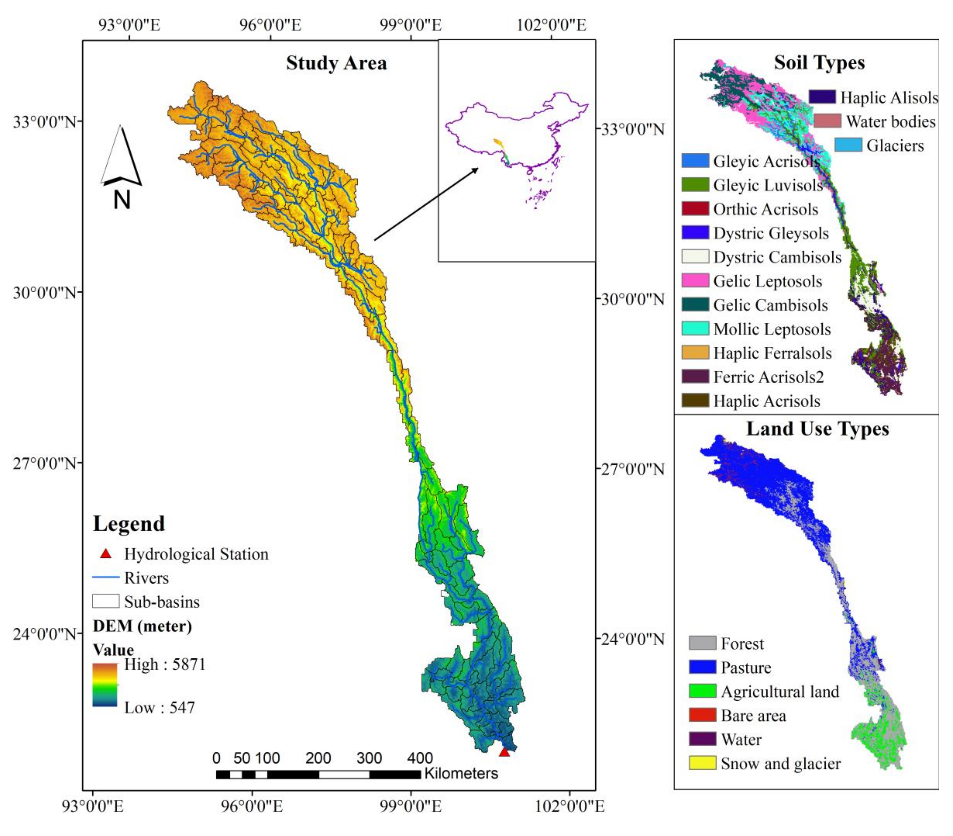
The LR is located in the southwestern region of China (Figure 1) and originated from the northeast slope of the Tanggula Mountains; it flows approximately 2140 km through Qinghai Province, Tibet Autonomous Region, and Yunnan Province of China from north to south, with a total drainage area of approximately 142,000 km2 [32,36]. It has an average elevation of approximately 3387 m, showing significant topographical characteristics of high north and low south. In the Qinghai–Tibet Plateau in the northern part of the basin, its elevation can reach 5871 m, while the lowest elevation in the lower plain area is only 547 m.
The climate of the LR Basin is regulated by the Indian monsoon system and westerlies monsoon with a mean annual precipitation ≈870 mm based on time series provided by the China Gauge-based Daily Precipitation Analysis (CGDPA) from 1961 to 2015. The precipitation in the basin has an extremely uneven spatial distribution, the annual precipitation in the Qinghai–Tibet Plateau in the northern part of the basin is only 400 mm, while it can be as high as 1800 mm in the southern plain. The monsoon climate causes the precipitation in the basin to show significant seasonal characteristics, which brings abundant water vapor and precipitation to the basin from June to September, accounting for ≈70% of the annual precipitation [31]. Correspondingly, the streamflow of the LR basin is mostly concentrated in June to October, and other months are the dry seasons [37].
The soil types in the upper reaches of the LR Basin are mainly Gelic Leptosols and Mollic Leptosols, and the lower reaches are mainly Dystric Cambisols and Ferric Acrisols. The land-use types in the LR Basin are mainly pasture, forest land, and agricultural land. Pasture is mainly distributed in high-altitude areas in the upper reaches, while forest and agricultural land are mainly distributed in the lower reaches of the LR Basin (Figure 1).
2.2. Datasets
2.2.1. Geographical Data
The Digital Elevation Model (DEM) of the Shuttle Radar Topography Mission with a 90 m resolution was used for the SWAT model development (http://srtm.csi.cgiar.org/). The soil dataset with ≈1 km resolution used in this study is Harmonized World Soil Database version 1.2 (HWSD v1.2), and it was obtained from the Food and Agriculture Organization (FAO) of the Untied State [38], which was further reclassified into 16 types using the ArcGIS tool (Figure 1). The land-use and land-cover change (LUCC) data with a resolution of ≈1 km was downloaded from the Global Land Cover 2000 (GLC2000) (http://bioval.jrc.ec.europa.euproducts/glc2000/products.php), and it has been reclassified into five types according to the database provided by SWAT model (Figure 1). The reclassification of soil and land-use data was conducted to meet the data requirements of the SWAT model and to reduce the complexity of model calculations.
2.2.2. Meteorological Data
The daily meteorological dataset was obtained from the China Gauge-based Daily Precipitation Analysis (CGDPA), which was developed by the National Meteorological Information Center of China Meteorological Administration [39,40]. This dataset was generated based on ≈2400 gauge observations from 1955 to almost the present over Mainland China using the optimal interpolation method [39]. A CGDPA series of datasets can provide daily precipitation, maximum and minimum temperature, relative humidity, and wind speed with a spatial resolution of 0.25, which are also required input data for streamflow simulation of a SWAT model. Previous studies have successfully applied CGDPA products to hydrometeorological research in many regions of China [18,41,42]. In this study, we entered each grid point of the CGDPA product with the period from 1973 to 2004 as a virtual station into the SWAT model.
The daily streamflow data of the Yunjinghong hydrometric station (Figure 1) from 1973 to 2004 were obtained from The Ministry of Water Resources of the People’s Republic of China and the local water management department.
2.3. SWAT Model
SWAT is a process based, semi-distributed hydrologic model which was developed by The Agricultural Research Service of the United States Department of Agriculture (USDA-ARS) to assess the impact of water resource management policies and non-point source pollution [43,44], and it has been widely used for flood forecasting [15], flood risk management, water resources assessment [17], and climate change impact on water resources [6,45] all over the world. In addition to its proven ability to simulate streamflow and assess other water quantity and quality problems, the SWAT model has already been chosen by The Mekong River Commission as part of its hydrological modeling tools since 2010 [46]. More detailed information about the SWAT model can be found in other literature.
The SWAT Version 2012 model coupled with the ArcGIS10.2 user interface was used to set up and parameterize in this study, and it was set up for the LRB over Yunjinghong station with the meteorological datasets mentioned above from 1973 to 2004. The LRB had been divided into 172 sub-basins (Figure 1) based on the DEM and gradient data, and further into 625 Hydrologic Response Units (HRUs) according to the information of soil, LUCC, water resources management, and topographical characteristics [1]. The categories of gradient data used were 0–5%, 5–10%, 10–15%, and >15% in the definition of each HRU. Five elevation bands were set in in this study to adjust the precipitation and temperature based on the sub-basin elevation changes [47]. The soil and LULC data were reclassified into 14 and six types, respectively based on the database provided by the SWAT model itself.
2.4. Uncertainty Analysis Methods
The uncertainty analysis methods (SUFI-2, GLUE, ParaSol, and PSO) used in this study are included in the SWAT-CUP (SWAT Calibration and Uncertainty Programs) platform [13]. A brief introduction to these uncertainty analysis methods is provided in this section, and more detailed information on these methods can be found in other literature [14,21].
2.4.1. SUFI-2
The Sequential Uncertainty Fitting procedure version 2 (SUFI-2) was developed by Abbaspour et al. [14], which is based on a Bayesian framework [5,48]. In the SUFI-2 method, the uncertainties of the parameters mainly include three aspects: the uncertainty of the input data sets, the model structure, and the measured data. The degree of uncertainty is primarily measured by the P-factor, which is usually expressed as 95 PPU (indicating the cumulative distribution of the simulated variable at the 2.5% and 97.5% levels, that is, 95% prediction uncertainty), and it represents the percentage of observed data enveloped by the 95PPU band [16]. The 95PPU uses the Latin hypercube sampling (LHS) method [49] to select the simulated value of the variable between 2.5% and 97.5%, and this value also excludes the worst 5% of cases. LHS is a stratified sampling technique, which requires approximate random sampling from the multi-parameter distribution to ensure that the sample structure is similar to the overall structure, thereby improving the accuracy of the estimation [50]. In addition, another measure to quantify the strength of uncertainty analysis is the R-factor, which is the ratio of the 95PPU width to the standard deviation. The main purpose of SUFI is to measure the uncertainty of the measured data and minimize the parameter interval. In general, SUFI first assumes a relatively large set of parameter intervals, so that the measured data are bracketed by the 95PPU, thereby narrowing the parameter range, and reducing the uncertainty interval. Finally, the three different objective functions (e.g., Nash–Sutcliffe efficiency coefficient (NSE), deterministic coefficient (R2), relative error (RE)) can be used for further simulation and study.
2.4.2. ParaSol
The Parameter Solution (ParaSol) algorithm was developed based on the Shuffled Complex Evolution (SCE-UA) method [29], which reduces the objective functions (OFs) and the global optimization criterion (GOC) by integrating the OFs into GOC to implement model calibration and uncertainty analysis. The SCE-UA algorithm is a global optimization method that minimizes one specific objective function with a maximum of 16 calibrated parameters [29]. This method combines the direct search principle of the simplex method with the controlled random search proposed by Nelder and Mead [51], which is a systematic evolution of parameter sets in searching for global improvement, complex shuffling, and competitive evolution [52]. In the process of SCE-UA execution, an initial population is first randomly generated within a reasonable range of p parameters to be adjusted; then, this initial group is divided into several complexes that consist of 2p + 1 points. Then, each complex evolves independently using the simplex algorithm based on the value of the objective function. To share information among each complex, these complexes are periodically reorganized to form new complexes. After the calibration of ParaSol, all the simulation results are divided into “good” and “not good” simulations according to a criterion value specified by a model user. ParaSol has been widely used for model calibration and uncertainty analysis and is generally found to be efficient and robust [21,53].
2.4.3. GLUE
Generalized Likelihood Uncertainty Estimation (GLUE) is a Monte Carlo simulation process based on the concept of multi-finality for some parameter sets that was developed by Beven and Binley [25]. This method takes the likelihood value of the alternative parameter value as the relative fitting ability of the parameter set to the measured data. The GLUE method is easy to implement, and it assumes that there is no unique optimal parameter set in the case of large over-parameterized hydrological models. The subjective likelihood measure is used to generate a posterior probability function and estimate the weights associated with each different calibrated parameter set, which are then used to estimate the predictive uncertainty of the output variables [19]. In addition, similar to the ParaSol method, the GLUE algorithm also divided the simulation results into “good” or “not good” by comparing the NSE with the threshold value set by the user [19,21], and the uncertainty analysis can also be performed using the P-factor and R-factor. Currently, the GLUE method has increasingly been used for the calibration of hydrological models and parameter uncertainty analysis [53,54].
2.4.4. PSO
The Particle Swarm Optimization algorithm (PSO) is a group-based optimization method first proposed by Kennedy and Eberhart in 1995 [30]. This method has been widely used in various industries because it is easy to implement and does not require gradient information [55]. It can also be used to solve a variety of optimization problems, including most problems that can be solved using genetic algorithms, and it can also solve some applications including neural network training and functional minimization. Initially, based on the value of the objective function, certain particles are identified as the best particles. Then, all the particles are accelerated in the direction of the particle, which is the direction of their own best solution they have previously found. Sometimes, particles go beyond the target and search beyond the current optimal particle search space, in which case all particles have a chance to find better particles so that the other particles will change direction and face the new “best” particles [55]. Since most features have a certain degree of continuity, a good solution may be surrounded by an equally good or better solution. By approaching the current best solution from different directions in the search space, these neighboring solutions are highly likely to be discovered by certain particles. Since PSO was created, it has been increasingly applied to the parameterization of hydrological models, the uncertainty analysis of hydrological model parameters, and reservoir scheduling [55,56,57].
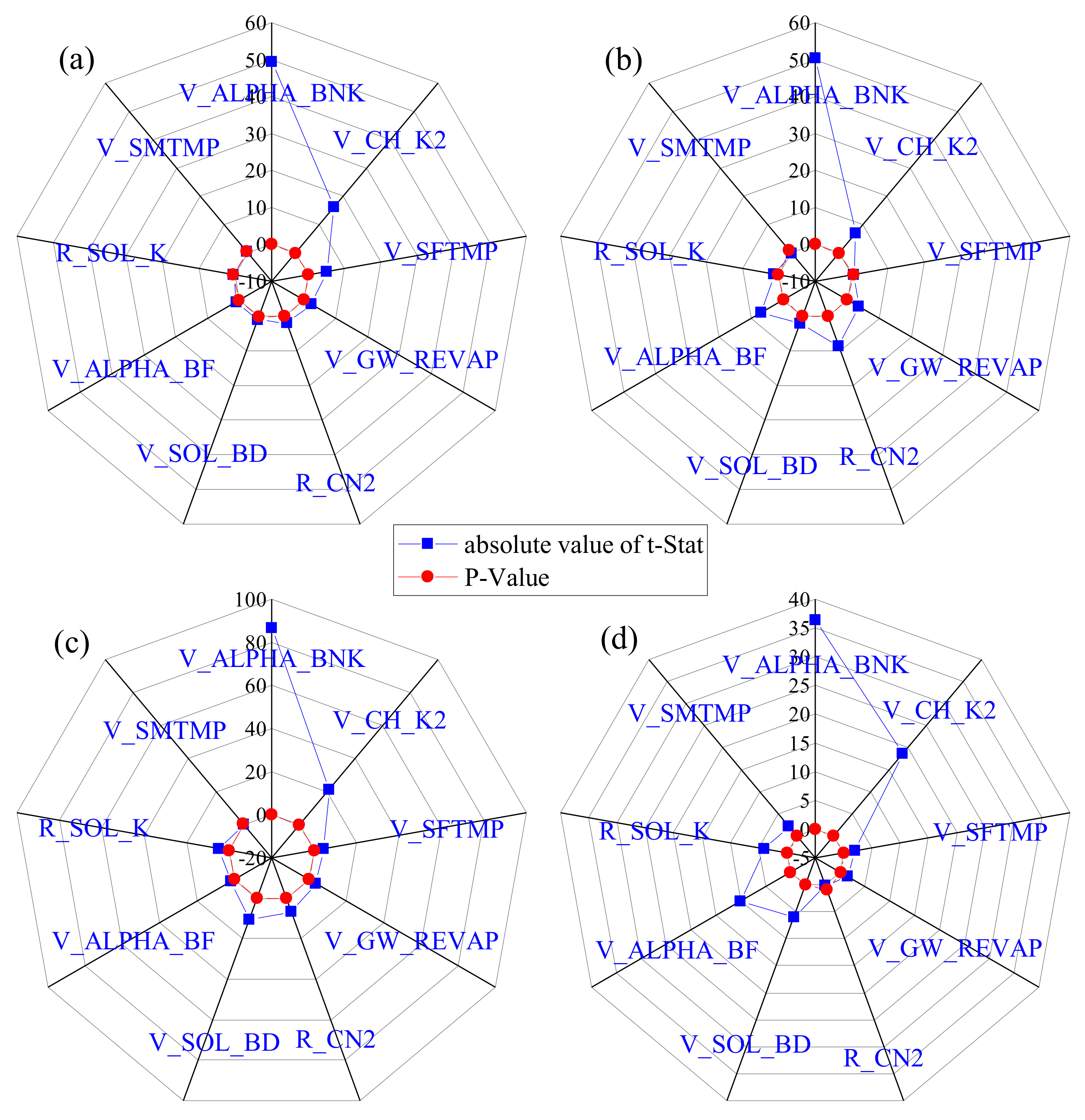
Before the uncertainty analysis, we first used the above four methods to identify the key parameters of the model’s streamflow simulation in the Lancang River basin and conducted a global sensitivity analysis of the parameters. In the procedure of the global sensitivity analysis, parameter sensitivities were described as a multiple regression system that was subsequently used to obtain the statistical value of the parameter sensitivity. A t-test (Student’s t-distribution) was used to calculate the relative significance of each calibrated parameter, and the t-Stat, which means a parameter divided by its standard error, was used to evaluate the parameter sensitivity. The P-value was another indicator used to evaluate the uncertainty, and this value measures the null hypothesis of the t-test that the coefficient has no effect (equal to zero). In general, a parameter with a large t-Stat value and a small P-value suggests that it has a higher sensitivity [5,52].
In order to evaluate the performance of the hydrologic model, Nash–Sutcliffe efficiency coefficient (NSE) [58], coefficient of determination (R2) and relative error (RE) were used. In the process of evaluating the uncertainty of the model, we applied two indictors including P-factor and R-factor [21]. Equations and their perfect values are listed in Table 1.
3. Results
3.1. Global Sensitivity Analysis
Before calibrating the SWAT model, nine parameters (Table 2) that control different hydrological cycles were selected based on previous publications [23,47,54] to implement the global sensitivity analysis by using the SUFI-2, ParaSol, GLUE, and PSO methods. In the parameter selection process, we mainly refer to the results in the research area that has similar characteristics of runoff generation and convergence with the LR Basin. It should be pointed out that we performed 2000, 3000, 5000, and 3000 simulations in SUFI-2, ParaSol, GLUE, and PSO, respectively, according to the recommendations of previous studies [16,53]. The sensitivity ranking of the nine parameters and the corresponding p-value and absolute value of t-Stat values are shown in Figure 2. As can be seen from Figure 2, the four algorithms all recognized that parameter ALPHA_BNK (Baseflow alpha factor for bank storage) had the highest sensitivity in the streamflow simulation of the LR basin, followed by CH_K2, which was the effective hydraulic conductivity in the main channel alluvium. In other published studies related to parameter sensitivity, the ALPHA_BNK and CH_K2 were also found to have high sensitivity in streamflow simulations in the same or similar research areas [18,59]. The third sensitivity parameters identified by the four methods of SUFI-2, ParaSol, GLUE, and PSO were SFTMP, GW_REVAP, SOL_BD, and ALPHA_BF, respectively, and the other six parameters showed relatively lower sensitivity for streamflow simulation. At the same time, we can see that SFTMP was also highly sensitive, indicating that snowmelt streamflow plays an important role in the LR basin [60]. Table 2 shows the physical meaning and initial range of values of the nine selected parameters as well as the optimal simulation values obtained by the four methods. It can be seen from Table 2 that the optimal parameter combination values obtained by different methods were quite different from each other. In general, through the above analysis results, the SUFI-2, ParaSol, GLUE, and PSO all can be used for parameter sensitivity analysis of streamflow simulation in the LR basin, and they can identify the key parameters (ALPHA_BNK and CH_K2) of streamflow simulation in this area.
3.2. Simulation Results
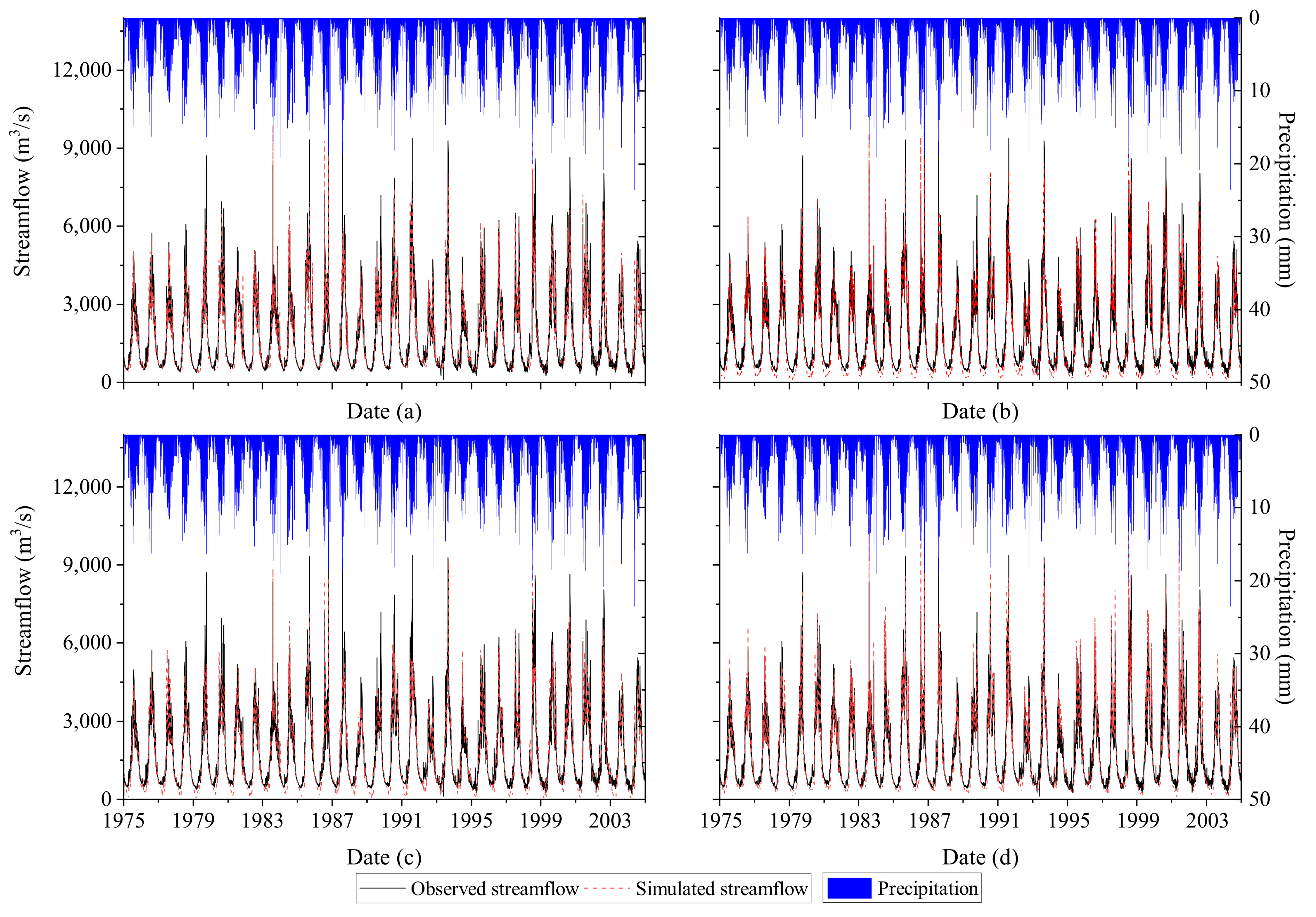
Using daily precipitation, maximum temperature, minimum temperature, wind speed, and relative humidity from 1973 to 2004, we compared the optimal simulation results derived from SUFI-2, ParaSol, GLUE, and PSO with the daily observed streamflow. In order to reduce the influence of the initial values of the model parameters on the simulation results, 1973 and 1974 were used as the warm-up period, 1975 to 1989 were used as the calibration period, and 1990 to 2004 were used for validation. Figure 3 shows the comparison of the observed streamflow and the best simulation for the Yunjinghong station at daily scale, and the optimal model evaluation metrics derived from the four algorithms are listed in Table 3. As can be seen from Figure 3, the simulated streamflow by using these four methods could all capture the daily streamflow process, but the parameter sets derived from the four methods were not in exact accordance with each other (Table 2), which meant that these four different algorithms could search for different combinations of parameters with similarly good simulations. As shown in Table 3, the model evaluation metrics of the four methods were all excellent in the calibration, validation, and the whole periods (NSE and R2 were both above 0.8, and RE was below 10%). According to the recommended standards in Moriasi et al. [61], the performance of the models obtained by the four methods has reached “very good performance”. In general, from the performance of different methods, the NSE and R2 values calibrated by ParaSol were the largest, followed by SUFI-2, GLUE, and PSO in the calibration and validation periods at a daily scale. From the perspective of RE, the simulated streamflow in both the calibration and validation periods was slightly overestimated compared with the observed streamflow (with a positive RE value), but these REs were all below 10%. In summary, compared with the other three methods, ParaSol had its own unique advantages in searching for the optimal parameter set to yield the best simulated streamflow.
3.3. Uncertainty Analysis in Streamflow Simulation
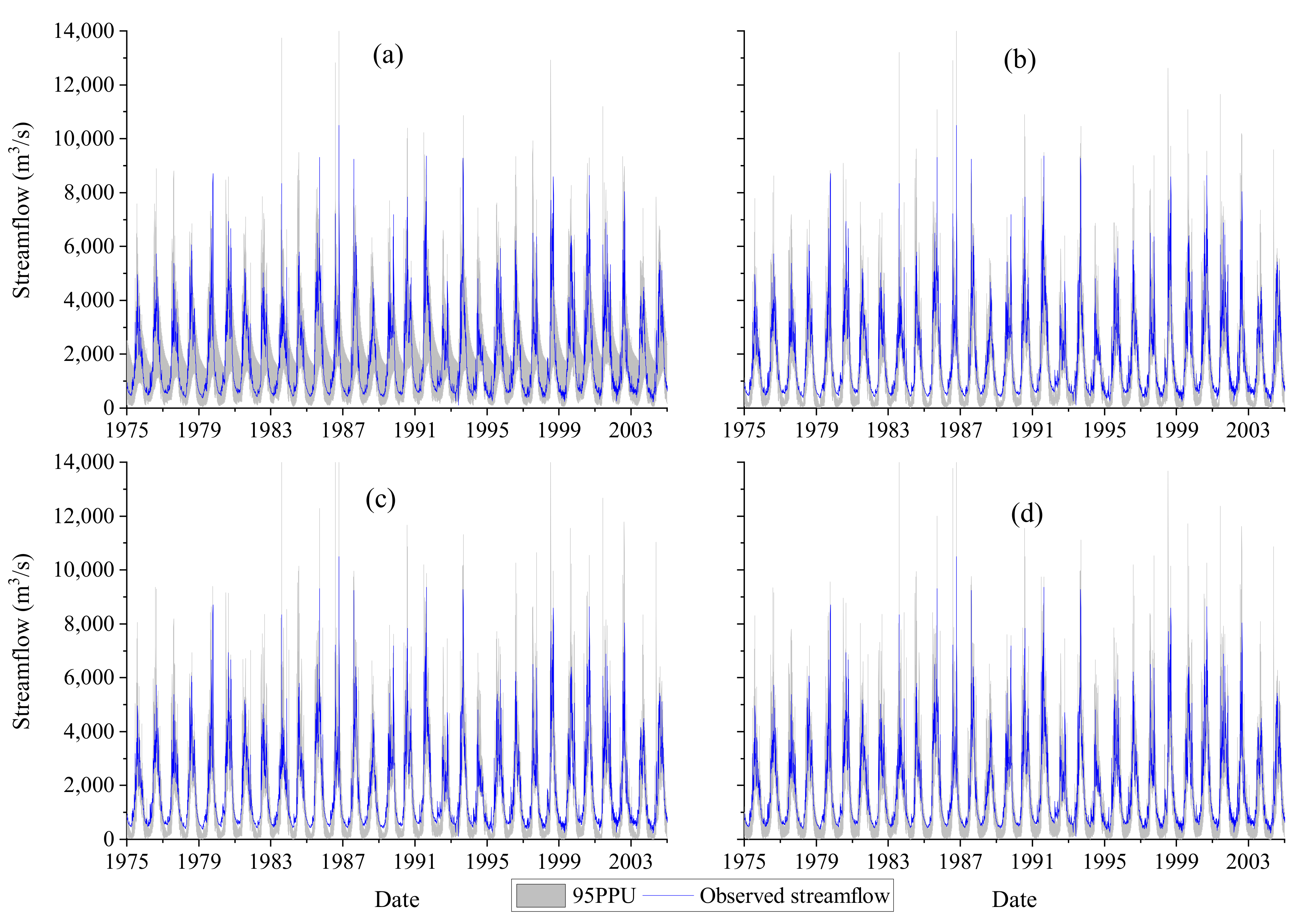
The model simulation uncertainty (95PPU) and metric values to evaluate the prediction uncertainty at daily scale derived from SUFI-2, ParaSol, GLUE, and PSO are shown in Figure 4 and Table 4. We can clearly see from Figure 4 that the 95PPU obtained by the SUFI-2 method was significantly greater than the other three methods over the calibration (P-factor = 0.92), validation (P-factor = 0.94), and whole periods (P-factor = 0.93), indicating that SUFI-2 had a significant advantage in the uncertainty analysis of streamflow simulation. For the other three methods, the thickness of 95PPU of PSO (P-factor = 0.78) was greater than that of GLUE (P-factor = 0.66). While the 95PPU of ParaSol was the smallest (P-factor = 0.51), this also indicated that although ParaSol had certain advantages in finding the optimal simulation parameter set (Figure 3 and Table 3), it was insufficient to apply it to the uncertainty analysis of runoff simulation. In general, the scope of the uncertainty evaluation indicators proposed by Abbaspour [52], that is, P > 0.7 and R < 1.5, are treated as acceptable performance in terms of streamflow prediction uncertainty. The SUFI-2 and PSO methods can be used for uncertainty analysis in the LR basin at daily scale. Among them, the SUFI-2 method was better than PSO, because its P-factor value was much larger than that of PSO.
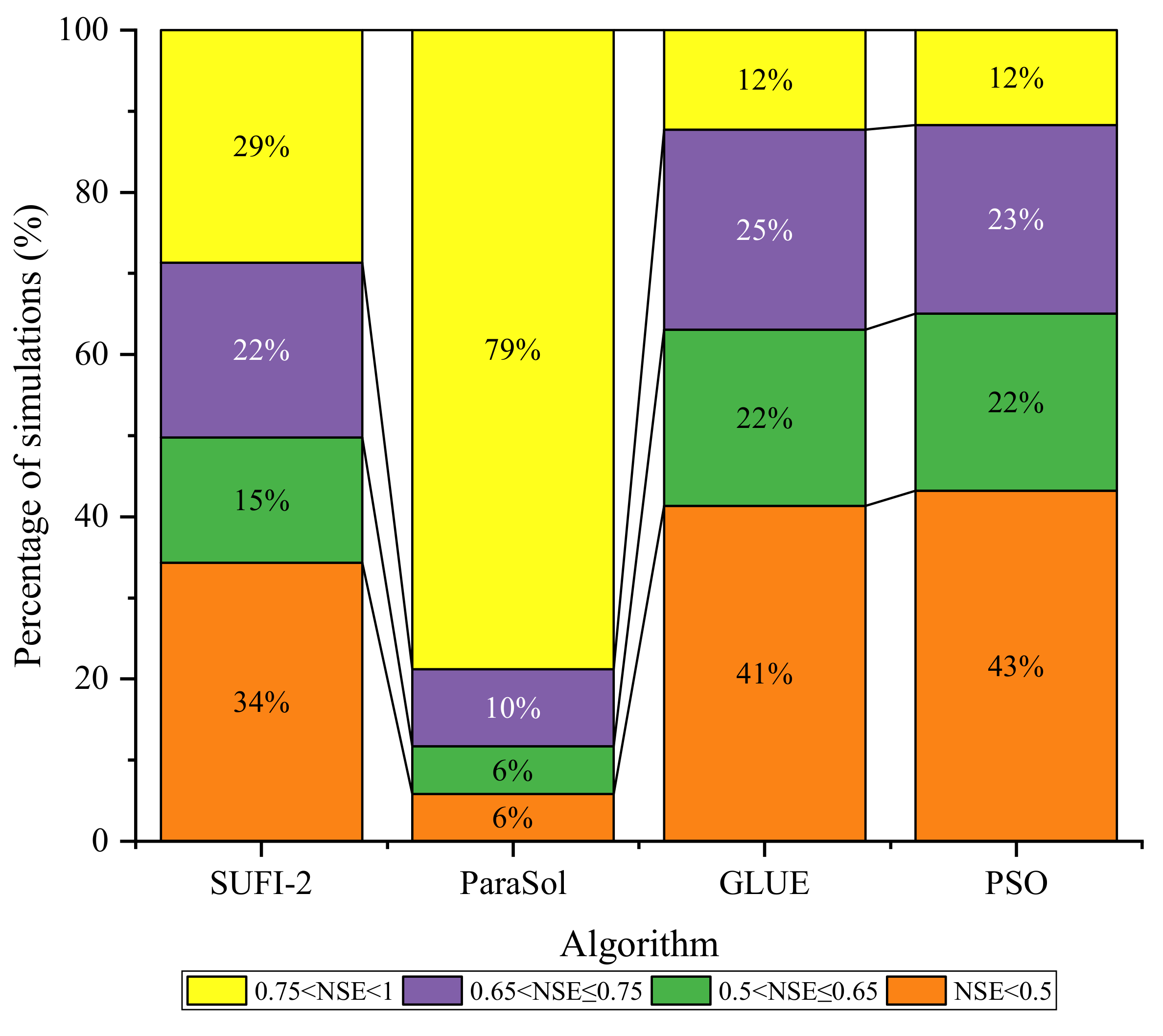
To further evaluate the ability of these four algorithms for the uncertainty analysis in streamflow simulation, according to the hydrological simulation evaluation index classification recommended by Moriasi et al. [61] (0.75 < NSE ≤ 1, 0.65 < NSE ≤ 0.75 and 0.5 < NSE ≤ 0.65 respectively represent the simulation results “satisfactory”, “good”, and “excellent”), we counted the frequency (%) and number of all simulation results of the four methods falling within different NSE value intervals (Figure 5 and Table 5). It can be seen from Figure 5 and Table 5 that out of 3000 simulations of the ParaSol algorithm, 2363 simulations (accounting for 79%) were excellent. This was because the SCE-UA algorithm used in ParaSol would adjust the evolution direction of the parameter combination according to the objective function value in real time, which led this algorithm to have the most simulations with NSE greater than 0.75. As for the GLUE algorithm, it had 2067 times (41%) of simulation results that perform poorly (NSE < 0.5), and only 615 times (12%) of simulation results with NSE greater than 0.75. This was mainly since the GLUE algorithm considered the uncertainties of multiple sources of hydrological simulation (hydrological model, meteorological input, etc.), resulting in a relatively large parameter combination interval. Meanwhile, PSO only had 352 times (11.7%) simulation results with NSE greater than 0.75, which was the worst performance among the four methods. This was mainly determined by the structure of the algorithm, because this algorithm was a random search algorithm that simulates the predation behavior of birds, which made the algorithm easy to fall into local optimal solutions [30]. The SUFI-2 algorithm also showed excellent streamflow simulation capabilities. In the 2000 simulations, a total of 573 simulations (29%) had an NSE greater than 0.75, and a total of 1313 simulations (33%) were “satisfactory”. In summary, the ParaSol algorithm presented a good performance in streamflow simulation, with more simulation results showing “excellent” (NSE > 0.75), followed by SUFI-2, PSO, and GLUE.
3.4. Uncertainty Analysis in Model Parameters
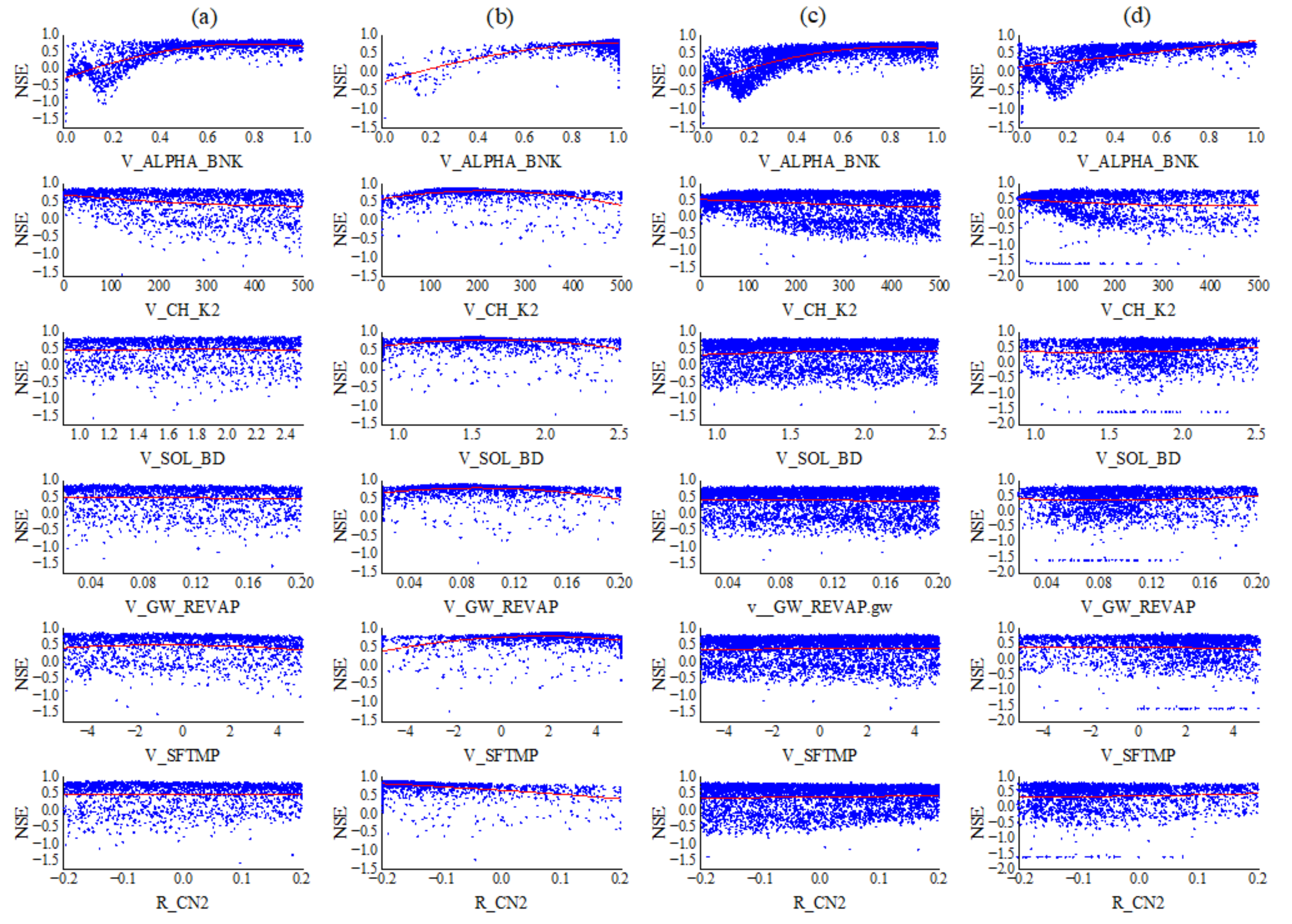
The distribution of different parameters yielded by SUFI-2 (a), ParaSol (b), GLUE (c), PSO (d) (the top six parameters in sensitivity ranking) and their corresponding NSE value scatter plots are shown in Figure 6. It can be seen from Figure 6 that the different combinations of the six parameters had a significant impact on the NSE value. The values of the most sensitive parameter ALPHA_BNK and NSE showed a class-exponential distribution in statistical significance, and its correlation with NSE was significant, especially in the interval of −0.5 < NSE < 0.5, but there was no obvious correlation in the interval of NSE greater than 0.5. In general, with the increase of ALPHA_BNK, NSE showed an increasing trend. As for the CH_K2 parameter with the second sensitivity ranking, when it was in the interval of 0–100, the NSE had the larger value, and when the value was greater than 100, the NSE showed a decreasing trend. The correlation between the parameter SOL_BD and the NSE value was generally very weak. For the GW_REVAP parameter, the values yielded by the SUFI-2 and ParaSol methods had a small negative correlation with the NSE; with the increase of the parameter, the NSE gradually decreases. The correlation coefficients presented by the four methods of parameter CN2 were similar to those of GW_REVAP. Within the parameter range we set, some parameter combinations had obtained poor simulation results (NSE was around −1.5), but at the same time, the ParaSol method obtained the best simulation results (NSE = 0.90, R2 = 0.92), and the optimal simulation results obtained by the other three methods were also relatively good. The combination of these parameters with poor simulation results may lead to a relatively large value of 95PPU. At the same time, in the parameter combination with a large NSE, the common phenomenon of “equifinality for different parameters” in hydrological simulation could be found; that is, different parameter combinations have achieved similar and identical objective function values.
Table 6 shows the correlation matrix between the parameter combinations calculated by SUFI-2, ParaSol, GLUE, and PSO. It can be seen from Table 6 that the correlations between the different parameter combinations produced by the four methods were obviously different. In general, the correlation between the parameter combinations generated by the ParaSol algorithm was relatively obvious, CH_K2 and CN2 (0.36), CH_K2 and GW_REVAP (0.34), CH_K2 and SOL_BD (0.29), CN2 and GW_REVAP (0.26), ALPHA_BNK and SFTMP (0.24), ALPHA_BNK and SOL_K (0.21) all showed positive. CN2 and ALPHA_BNK, SOL_BD and SMTMP, SMTMP and CN2 were negatively correlated, and their correlation coefficients were −0.47, −0.32, and −0.31, respectively. The correlation between the different parameters produced by the PSO algorithm was weaker than that produced by the ParaSol algorithm. The combination of parameters generated by the SUFI-2 algorithm and the GLUE algorithm had less correlation with each other, which made it more reasonable for the two algorithms to analyze the sensitivity of hydrological model parameters and the hydrological simulations. Conversely, this also caused the optimal simulation results obtained by these two algorithms to be slightly worse than the results obtained by the ParaSol algorithm.
Table 7 shows the 95PPU value of the parameter combination obtained by the four methods of SUFI-2, ParaSol, GLUE, and PSO. It can be seen from Table 7 that within given initial parameter ranges, among the parameter sets obtained by the two methods of SUFI-2 and GLUE, the 95PPU of these two parameter sets was relatively close, and it was larger than that derived from ParaSol and PSO. Among them, the parameter ranges generated by ParaSol were the smallest. This was because in the process of optimizing model parameters for the ParaSol algorithm, it constantly updates the parameter combination according to the optimal value of the objective function. Therefore, the ParaSol algorithm could achieve better streamflow simulation results (Table 3). The parameter ranges generated by the PSO algorithm were larger than those generated by ParaSol. This was due to the limitation of the algorithm itself, in the case of convergence, because all particles “fly” in the direction of the optimal solution (the objective function value was the largest). This will cause the updated parameter group to tend to be the same, which will slow down the convergence speed in the later stage and cannot continue to optimize. This was also one of the main reasons why the streamflow simulation result of the PSO algorithm was slightly worse than those of the other algorithms. As for the SUIF-2 and GLUE algorithms, because these two methods consider the uncertainties of hydrological models and other aspects in the process of optimizing streamflow simulation parameters, the range of parameters generated by the two methods was relatively large. In general, SUFI-2 and GLUE have greater advantages in the uncertainty analysis of model parameters, while the PSO and ParaSol algorithms have certain limitations, although the ParaSol algorithm can obtain larger NSE and R2 values.
3.5. Water Balance Components Analysis
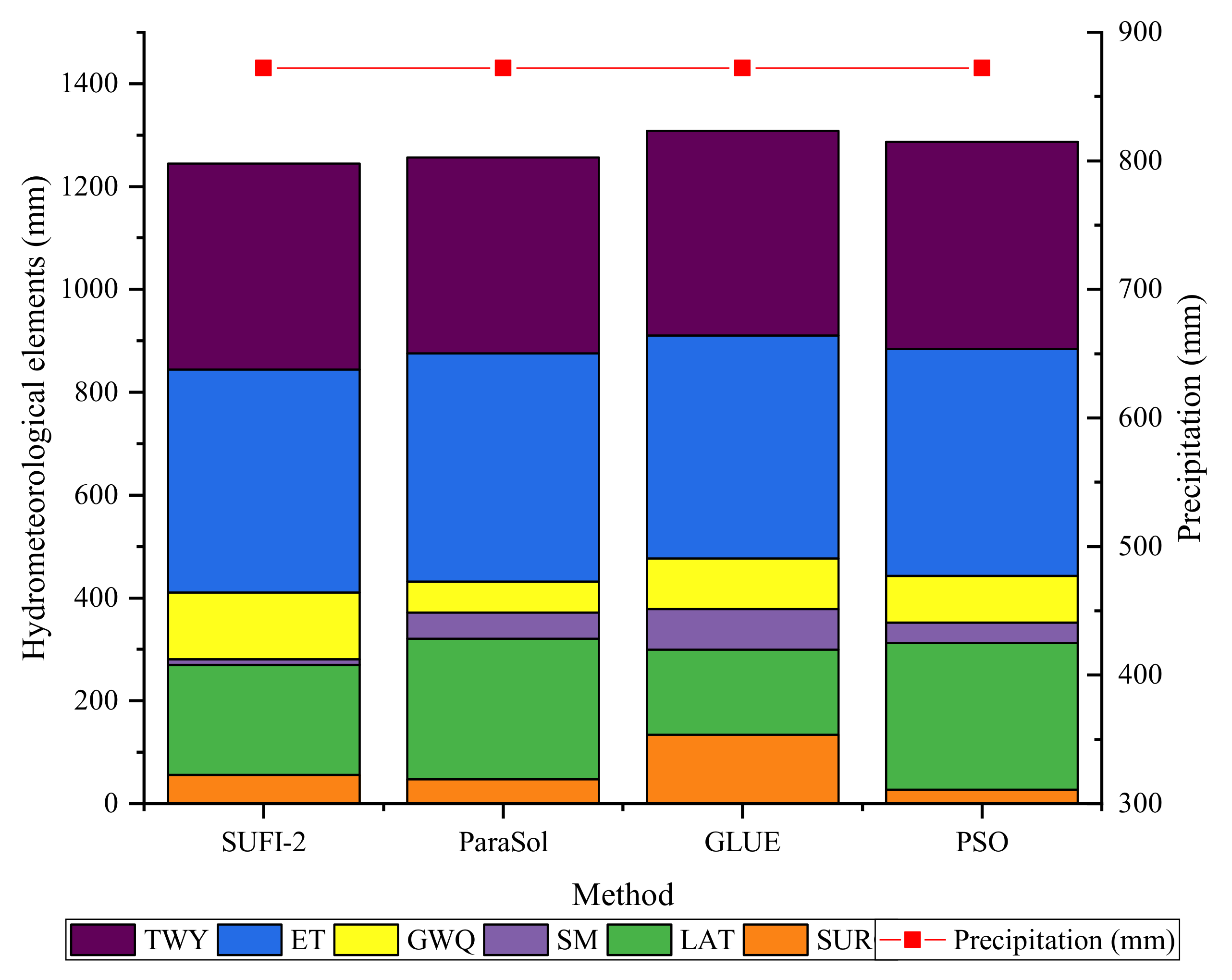
In the process of hydrological model calibration, the model often adjusts the other variables to make the variables we want to calibrate close to the measured variable. Table 8 shows the average contributions to the water balance for the main hydrological components at the Yunjinghong station using the SUFI-2, ParaSol, GLUE, and PSO algorithms with the optimal parameter sets (Table 2). From 1975 to 2004, the average annual precipitation was 872.2 mm, as predicted by CGDPA. It was worth noting that the actual evapotranspiration (ET) values predicted by the four methods were not much different from each other, suggesting that the actual evapotranspiration calculated using these four different algorithms had the least uncertainty. In addition to the ET variable, the other main hydrological components differ greatly among the different algorithms. For the surface runoff (SURQ), CN2 controlled the SURQ of the watershed, and the CN2 value that was derived from the GLUE algorithm was much larger than that of the other three algorithms (Table 2) to the results showed a large surface runoff for GLUE, followed by ParaSol, PSO, and SUFI-2. ALPHA_BNK, SOL_K, and SOL_BD mainly affected the base flow and groundwater runoff (GWQ) of the river. The GWQ calculated by SUFI-2 was larger than that derived from the other three methods. The GWQ calculated by ParaSol and GLUE was quite different, but the values for their most sensitive parameter, ALPHA_BNK, were relatively close (Table 2), which meant that the parameters did not affect streamflow generation separately, and the joint effects between different parameters would affect the quantities of different hydrological components in the basin. For snowmelt runoff (SM), the calculation result of GLUE was significantly greater than those of the other three methods. This was mainly controlled by two snowmelt parameters (SFTMP and SMTMP). The SFTMP calculated by GLUE was 4.0 °C, which was significantly larger than the other three methods, and it meant that more precipitation exists in the form of snowfall, while SMTMP was the smallest, indicating more snow has been melted. Figure 7 shows the multi-year average variation in different hydrological components derived from the SUFI-2, ParaSol, GLUE, and PSO methods from 1975 to 2004. From 1975 to 2004, the actual evapotranspiration (ET) calculated by the four algorithms accounts for less than half of the precipitation. In addition to the actual evapotranspiration (ET), the calculation results of the four methods all showed that lateral flow (LAT) accounts for the largest proportion of streamflow formation in the basin.
4. Discussion
To obtain better simulation results, it is important to identify the sensitivities of the key parameters before calibrating a model. In this study, global sensitivity analysis was implemented to identify the nine most sensitive parameters from the streamflow simulation with 25 selected parameters. As shown in Table 1, ALPHA_BNK and CH_K2 were identified as more sensitive than the other seven parameters. These two parameters were also found to be more sensitive in other published studies [59]. It should be pointed out that CN2 was found to have low sensitivity in this study, and some published studies showed that its sensitivity was high [21,53], because CN2 mainly controls the surface runoff process of the watershed, and in this study area, the contribution of surface runoff to the entire runoff was relatively small. The model performance calibrated by using the four algorithms is shown in Table 3. In terms of the model evaluation indicators, the ParaSol method had slightly higher NSE and R2 values as well as a small RE value than the other three methods in the calibration, validation, and the whole periods at daily scale, suggesting that this method had its own advantages in searching for the global optimal solution. This finding was consistent with the findings of other published papers [21,27]. This is mainly because ParaSol combines the advantages of deterministic search, random search, and biological competitive evolution, and it can adjust the evolution direction of the parameter combination according to the objective function value in real time and then seek the global optimal solution [21,27,29]. Therefore, we recommend that the ParaSol algorithm can be used preferentially to search for the optimal combination of parameters in the streamflow simulation over the Yunjinghong station compared with the other three methods. From Figure 3, we can also clearly see that the optimal simulation results obtained by ParaSol, GLUE, and PSO show different degrees of underestimation in the dry season (from March to May), which is also the reason for the large relative error (RE) of the simulation. The reason for this phenomenon may be the influence of the SWAT model’s own snowmelt module, which uses only a simple degree-day factor model to estimate the snowmelt process [44]. Another reason may be the impact of water transfer in the dry season of the main stream reservoir of the LR Basin. Of course, due to the complex topographic features of the study area, CGDPA meteorological data may also bring certain uncertainty to the streamflow simulation results [41].
For the model prediction uncertainty analysis, our study showed that SUFI-2 and PSO were better methods with relatively larger P-factors and smaller R-factors. For the uncertainty of the model parameters, our study showed that most calibrated parameters derived by ParaSol had narrower widths (95PPU) compared with the initial ranges, which suggested that ParaSol was less robust in implementing the uncertainty analysis for streamflow prediction. For the SUFI-2, GLUE, and PSO algorithms, the wider 95PPU of the parameters may be because these three methods considered multiple uncertainties, such as that of the parameters, model structure, and correlation between parameters, which may lead to relatively larger parameter uncertainties than those of the ParaSol method. We also compared the numbers of simulations of the four methods that were relatively good (with NSE greater than 0.5) (Figure 5 and Table 5). The ParaSol algorithm had 2825 (94%) simulation results with NSE coefficients greater than 0.5 in the whole period (1975 to 2004) and performed much better than the other three algorithms, while the PSO method had the least number (1703, 57%) of simulations with an NSE greater than 0.5; these results meant that ParaSol, which based on the SCE-UA algorithm, was very efficient in searching for the parameter set closest to the optimal value of the objective function (refer to the NSE coefficient) [21,27]. As pointed out by Yang et al. [54], the PSO algorithm easily falls into a local optimal solution when dealing with the optimal solution of discrete problems, which may lead to the poor performance of PSO in the uncertainty analysis of streamflow simulations.
We also compared the amounts of the different main hydrological components that were derived from the four algorithms with each optimal parameter set. We found that the actual evapotranspiration (ET) calculated by the four different algorithms was basically the same, while the other hydrological components differed greatly in the different methods (Table 8 and Figure 7), these findings suggested that although we obtained good simulation results for the streamflow, these simulation results also had large uncertainties for the components of the entire hydrological cycle [16,26]. The possible reason is that we mainly calibrate the model by fitting the simulated streamflow and the observed ones. In order to get better simulation results, the total water yield derived from the four methods is basically the same (Table 8). Based on the principle of water balance, the amount of actual evapotranspiration is not much different from each other. Due to lacking more measured data from the study area, we can adjust the model parameters by using remote sensing soil moisture and evapotranspiration to reduce the uncertainty of the model simulations in a follow-up study.
5. Conclusions
In this study, we evaluated the streamflow simulation capabilities and uncertainties of four uncertainty analysis algorithms (i.e., SUFI-2, ParaSol, GLUE, and PSO) through a semi-distributed hydrological model, the SWAT model, for a case study in the Lancang River (LR) Basin over the Yunjinghong station. The main conclusions are as follows:
(1) The global sensitivity analysis of the nine selected parameters indicated that all four methods could be used for parameter sensitivity analysis in the LR Basin, and all could identify the key parameters with higher sensitivity (ALPHA_BNK and CH_K2). Meanwhile, the sensitivity of the other seven parameters to streamflow simulation was relatively low. This result will have reference significance for the calibration of the hydrological model parameters of the basins, which has similar runoff generation and confluence characteristics with the LR Basin.
(2) The simulation results using the four algorithms showed that the streamflow process can be well simulated using the CGDPA meteorological product and the SWAT model in the LR Basin at the daily scale. Among the four methods, ParaSol had the best performance with NSE and R2 values of 0.89 and 0.92 for the calibration period, and 0.90 and 0.91 for the validation period, respectively, followed by SUFI-2, GLUE, and PSO. These results indicated that compared with the other three methods, ParaSol had specific advantages in seeking the optimal combination of parameters.
(3) The results of the uncertainty analysis showed that the SUFI-2 and PSO can achieve better results, and the performance of SUFI-2 was much better than PSO in terms of P-factor (0.93 vs. 0.78) and R-factor (1.17 vs. 1.14) values. For the uncertainty of the parameters, the ParaSol method had the smallest 95PPU thickness compared with the other three methods. For acceptable simulation times (NSE > 0.5), the ParaSol method had the most proportion simulation times, followed by SUFI-2, GLUE, and PSO.
(4) It could be seen from the analysis results of the main hydrological components of different methods that the actual evapotranspiration (ET) calculated by the four methods was relatively close, while the other hydrological components (such as Groundwater Runoff, Surface Runoff, Snow Melt, and Lateral Runoff) have large differences among the different methods.
Although some conclusions of this study can provide important references for hydrological simulation of basins with similar runoff and confluence characteristics to the LR Basin, this study still has certain limitations. In this study, we only consider the uncertainty of the average streamflow in the hydrological simulation, and we did not consider the impact of parameter uncertainty on the high and low flows, which are also of great significance to water resources management in the basin. On the other hand, this study did not consider the uncertainty of other hydrometeorological elements (such as soil moisture, etc.) related to the hydrological cycle. In addition, in a follow-up study, the high-resolution remote sensing soil moisture and evapotranspiration data can be used to calibrate the other main hydrological components of the water cycle, thus reducing the uncertainty of the simulation.
Author Contributions
This study was calculated and written by X.T.; G.W. designed the experimental framework of this work; J.Z., C.L., Y.L., R.H., Z.B. and J.J. contributed to the revision of manuscript and data collection. All authors have read and agreed to the published version of the manuscript.
Funding
This study was funded by National Natural Science Foundation of China (No. 41830863, 92047301, 51879162, 52079026), the National Key Research and Development Programs of China (No. 2016YFA0601501, 2017YFC0404401, 2017YFA0605002, 2017YFA0605002), the Belt and Road Fund on Water and Sustainability of the State Key Laboratory of Hydrology-Water Resources and Hydraulic Engineering (No. 2019nkzd02).
Institutional Review Board Statement
Not applicable.
Informed Consent Statement
Not applicable.
Data Availability Statement
The data presented in this study are available on request from the corresponding author or the first author.
Conflicts of Interest
The authors declare no conflict of interest.
References
- Abbaspour, K.C.; Rouholahnejad, E.; Vaghefi, S.; Srinivasan, R.; Yang, H.; Kløve, B. A continental-scale hydrology and water quality model for Europe: Calibration and uncertainty of a high-resolution large-scale SWAT model. J. Hydrol. 2015, 524, 733–752. [Google Scholar] [CrossRef] [Green Version]
- Li, D.; Long, D.; Zhao, J.; Lu, H.; Hong, Y. Observed changes in flow regimes in the Mekong River basin. J. Hydrol. 2017, 551, 217–232. [Google Scholar] [CrossRef]
- Wang, F.; Hessel, R.; Mu, X.; Maroulis, J.; Zhao, G.; Geissen, V.; Ritsema, C.J. Distinguishing the impacts of human activities and climate variability on runoff and sediment load change based on paired periods with similar weather conditions: A case in the Yan River, China. J. Hydrol. 2015, 527, 884–893. [Google Scholar] [CrossRef]
- Zhang, J.; Li, Y.; Huang, G.; Chen, X.; Bao, A. Assessment of parameter uncertainty in hydrological model using a Markov-Chain-Monte-Carlo-based multilevel-factorial-analysis method. J. Hydrol. 2016, 538, 471–486. [Google Scholar] [CrossRef]
- Abbaspour, K.C.; Johnson, C.A.; Van Genuchten, M.T. Estimating Uncertain Flow and Transport Parameters Using a Sequential Uncertainty Fitting Procedure. Vadose Zone J. 2004, 3, 1340–1352. [Google Scholar] [CrossRef]
- Ouyang, F.; Zhu, Y.; Fu, G.; Lü, H.; Zhang, A.; Yu, Z.; Chen, X. Impacts of climate change under CMIP5 RCP scenarios on streamflow in the Huangnizhuang catchment. Stoch. Environ. Res. Risk Assess. 2015, 29, 1781–1795. [Google Scholar] [CrossRef]
- Zeng, Q.; Chen, H.; Guo, S.; Jie, M.-X.; Chen, J.; Guo, S.-L.; Liu, J. The effect of rain gauge density and distribution on runoff simulation using a lumped hydrological modelling approach. J. Hydrol. 2018, 563, 106–122. [Google Scholar] [CrossRef]
- Bergström, S. The HBV Model—Its Structure and Applications; SMI-Il: Norrköping, Sweden, 1992. [Google Scholar]
- Liu, J.; Chen, X.; Zhang, J.; Flury, M. Coupling the Xinanjiang model to a kinematic flow model based on digital drainage networks for flood forecasting. Hydrol. Process. 2009, 23, 1337–1348. [Google Scholar] [CrossRef]
- Boughton, W.; Chiew, F. Estimating runoff in ungauged catchments from rainfall, PET and the AWBM model. Environ. Model. Softw. 2007, 22, 476–487. [Google Scholar] [CrossRef] [Green Version]
- Zhao, Q.; Liu, Z.; Ye, B.; Qin, Y.; Wei, Z.; Fang, S. A snowmelt runoff forecasting model coupling WRF and DHSVM. Hydrol. Earth Syst. Sci. 2009, 13, 1897–1906. [Google Scholar] [CrossRef] [Green Version]
- Bao, Z.; Zhang, J.; Wang, G.; Fu, G.; He, R.; Yan, X.; Jin, J.; Liu, Y.; Zhang, A. Attribution for decreasing streamflow of the Haihe River basin, northern China: Climate variability or human activities? J. Hydrol. 2012, 460, 117–129. [Google Scholar] [CrossRef]
- Atkinson, H.D.; Johal, P.; Falworth, M.S.; Ranawat, V.S.; Dala-Ali, B.; Martin, D.K. Adductor tenotomy: Its role in the management of sports-related chronic groin pain. Arch. Orthop. Trauma Surg. 2010, 130, 965–970. [Google Scholar] [CrossRef] [PubMed]
- Abbaspour, K.C.; Van Genuchten, M.T.; Schulin, R.; Schläppi, E. A sequential uncertainty domain inverse procedure for estimating subsurface flow and transport parameters. Water Resour. Res. 1997, 33, 1879–1892. [Google Scholar] [CrossRef] [Green Version]
- Zhu, Q.; Xuan, W.; Liu, L.; Xu, Y.-P. Evaluation and hydrological application of precipitation estimates derived from PERSIANN-CDR, TRMM 3B42V7, and NCEP-CFSR over humid regions in China. Hydrol. Process. 2016, 30, 3061–3083. [Google Scholar] [CrossRef]
- Tuo, Y.; Duan, Z.; Disse, M.; Chiogna, G. Evaluation of precipitation input for SWAT modeling in Alpine catchment: A case study in the Adige river basin (Italy). Sci. Total Environ. 2016, 573, 66–82. [Google Scholar] [CrossRef] [PubMed] [Green Version]
- Ruan, H.; Zou, S.; Yang, D.; Wang, Y.; Yin, Z.; Lu, Z.; Li, F.; Xu, B. Runoff Simulation by SWAT Model Using High-Resolution Gridded Precipitation in the Upper Heihe River Basin, Northeastern Tibetan Plateau. Water 2017, 9, 866. [Google Scholar] [CrossRef] [Green Version]
- Tang, X.; Zhang, J.; Wang, G.; Yang, Q.; Yang, Y.; Guan, T.; Liu, C.; Jin, J.; Liu, Y.; Bao, Z. Evaluating Suitability of Multiple Precipitation Products for the Lancang River Basin. Chin. Geogr. Sci. 2019, 29, 37–57. [Google Scholar] [CrossRef] [Green Version]
- Beven, K.; Freer, J.E. Equifinality, data assimilation, and uncertainty estimation in mechanistic modelling of complex environmental systems using the GLUE methodology. J. Hydrol. 2001, 249, 11–29. [Google Scholar] [CrossRef]
- Nešpor, V.; Sevruk, B. Estimation of Wind-Induced Error of Rainfall Gauge Measurements Using a Numerical Simulation. J. Atmos. Ocean. Technol. 1999, 16, 450–464. [Google Scholar] [CrossRef]
- Wu, H.; Chen, B. Evaluating uncertainty estimates in distributed hydrological modeling for the Wenjing River watershed in China by GLUE, SUFI-2, and ParaSol methods. Ecol. Eng. 2015, 76, 110–121. [Google Scholar] [CrossRef]
- Harmel, R.; Smith, P.; Migliaccio, K.; Chaubey, I.; Douglas-Mankin, K.; Benham, B.; Shukla, S.; Muñoz-Carpena, R.; Robson, B. Evaluating, interpreting, and communicating performance of hydrologic/water quality models considering intended use: A review and recommendations. Environ. Model. Softw. 2014, 57, 40–51. [Google Scholar] [CrossRef]
- Grusson, Y.; Sun, X.; Gascoin, S.; Sauvage, S.; Raghavan, S.; Anctil, F.; Sánchez-Pérez, J.M. Assessing the capability of the SWAT model to simulate snow, snow melt and streamflow dynamics over an alpine watershed. J. Hydrol. 2015, 531, 574–588. [Google Scholar] [CrossRef]
- Biondi, D.; Freni, G.; Iacobellis, V.; Mascaro, G.; Montanari, A. Validation of hydrological models: Conceptual basis, methodological approaches and a proposal for a code of practice. Phys. Chem. Earth Parts A/B/C 2012, 70–76. [Google Scholar] [CrossRef]
- Beven, K.J.; Binley, A.M. The future of distributed models: Model calibration and uncertainty prediction. Hydrol. Process. 1992, 6, 279–298. [Google Scholar] [CrossRef]
- Cao, Y.; Zhang, J.; Yang, M.; Lei, X.; Guo, B.; Yang, L.; Zeng, Z.; Qu, J. Application of SWAT Model with CMADS Data to Estimate Hydrological Elements and Parameter Uncertainty Based on SUFI-2 Algorithm in the Lijiang River Basin, China. Water 2018, 10, 742. [Google Scholar] [CrossRef] [Green Version]
- Zhao, F.; Wu, Y.; Qiu, L.; Sivakumar, B.; Zhang, F.; Sun, Y.; Sun, L.; Li, Q.; Voinov, A. Spatiotemporal features of the hydro-biogeochemical cycles in a typical loess gully watershed. Ecol. Indic. 2018, 91, 542–554. [Google Scholar] [CrossRef]
- Song, X.; Zhang, J.; Zhan, C.; Xuan, Y.; Ye, M.; Xu, C. Global sensitivity analysis in hydrological modeling: Review of concepts, methods, theoretical framework, and applications. J. Hydrol. 2015, 523, 739–757. [Google Scholar] [CrossRef] [Green Version]
- Duan, Q.; Sorooshian, S.; Gupta, V. Effective and efficient global optimization for conceptual rainfall-runoff models. Water Resour. Res. 1992, 28, 1015–1031. [Google Scholar] [CrossRef]
- Eberhart, R.; Kennedy, J. A new optimizer using particle swarm theory. In Proceedings of the MHS’95. Sixth International Symposium on Micro Machine and Human Science, Nagoya, Japan, 4–6 October 1995; Volume 10, pp. 1109–1995. [Google Scholar]
- Jacobs, J.W. The Mekong River Commission: Transboundary water resources planning and regional security. Geogr. J. 2002, 168, 354–364. [Google Scholar] [CrossRef]
- Han, Z.; Long, D.; Fang, Y.; Hou, A.; Hong, Y. Impacts of climate change and human activities on the flow regime of the dammed Lancang River in Southwest China. J. Hydrol. 2019, 570, 96–105. [Google Scholar] [CrossRef]
- Hecht, J.S.; Lacombe, G.; Arias, M.E.; Dang, T.D.; Piman, T. Hydropower dams of the Mekong River basin: A review of their hydrological impacts. J. Hydrol. 2019, 568, 285–300. [Google Scholar] [CrossRef]
- Hennig, T.; Wang, W.; Feng, Y.; Ou, X.; He, D. Review of Yunnan’s hydropower development. Comparing small and large hydropower projects regarding their environmental implications and socio-economic consequences. Renew. Sustain. Energy Rev. 2013, 27, 585–595. [Google Scholar] [CrossRef]
- Lauri, H.; De Moel, H.; Ward, P.J.; Rasanen, T.A.; Keskinen, M.; Kummu, M. Future changes in Mekong River hydrology: Impact of climate change and reservoir operation on discharge. Hydrol. Earth Syst. Sci. 2012, 16, 4603–4619. [Google Scholar] [CrossRef]
- Long, D.; Shen, Y.; Sun, A.; Hong, Y.; Longuevergne, L.; Yang, Y.; Li, B.; Chen, L. Drought and flood monitoring for a large karst plateau in Southwest China using extended GRACE data. Remote Sens. Environ. 2014, 155, 145–160. [Google Scholar] [CrossRef]
- MRC, M.R.C. Overview of the Hydrology of the Mekong Basin; Mekong River Commission: Vientiane, Laos, 2005. [Google Scholar]
- Nachtergaele, F.O.; Velthuizen, H.V.; Verelst, L.; Batjes, N.H.; Dijkshoorn, J.A.; Engelen, V.W.P.; Fischer, G.; Jones, A.; Montanarella, L. Harmonized World Soil Database (Version 1.2); FAO: Rome, Italy; IIASA: Laxenburg, Austria, 2012. [Google Scholar]
- Shen, Y.; Xiong, A. Validation and comparison of a new gauge-based precipitation analysis over mainland China. Int. J. Climatol. 2016, 36, 252–265. [Google Scholar] [CrossRef]
- Shen, Y.; Zhao, P.; Pan, Y.; Yu, J. A high spatiotemporal gauge-satellite merged precipitation analysis over China. J. Geophys. Res. Atmos. 2014, 119, 3063–3075. [Google Scholar] [CrossRef]
- Tang, G.; Long, D.; Hong, Y.; Gao, J.; Wan, W. Documentation of multifactorial relationships between precipitation and topography of the Tibetan Plateau using spaceborne precipitation radars. Remote Sens. Environ. 2018, 208, 82–96. [Google Scholar] [CrossRef]
- Yong, B.; Chen, B.; Tian, Y.; Yu, Z.; Hong, Y. Error-Component Analysis of TRMM-Based Multi-Satellite Precipitation Estimates over Mainland China. Remote Sens. 2016, 8, 440. [Google Scholar] [CrossRef] [Green Version]
- Arnold, J.G.; Kiniry, J.R.; Srinivasan, R.; Williams, J.R.; Haney, E.B.; Neitsch, S.L. Soil & Water Assessment Tool: Input/Output Documentation, Version 2012; Texas Water Resources Institute: College Station, TX, USA, 2012; pp. 1–650. [Google Scholar]
- Gowda, P.H.; Mulla, D.J.; Desmond, E.D.; Ward, A.D.; Moriasi, D.N. ADAPT: Model Use, Calibration, and Validation. Trans. ASABE 2012, 55, 1345–1352. [Google Scholar] [CrossRef]
- Lee, S.; Yeo, I.-Y.; Sadeghi, A.M.; Mccarty, G.W.; Hively, W.D.; Lang, M.W.; Sharifi, A. Comparative analyses of hydrological responses of two adjacent watersheds to climate variability and change using the SWAT model. Hydrol. Earth Syst. Sci. 2018, 22, 689–708. [Google Scholar] [CrossRef] [Green Version]
- MRC. Stage 2 Development of MRC Toolbox: Final Report (WP016); Information and Knowledge Management Programme; Mekong River Commission (MRC): Phnom Penh, Cambodia, 2010. [Google Scholar]
- Gan, R.; Luo, Y.; Zuo, Q.; Sun, L. Effects of projected climate change on the glacier and runoff generation in the Naryn River Basin, Central Asia. J. Hydrol. 2015, 523, 240–251. [Google Scholar] [CrossRef]
- Abbaspour, K.C.; Yang, J.; Maximov, I.; Siber, R.; Bogner, K.; Mieleitner, J.; Zobrist, J.; Srinivasan, R. Modelling hydrology and water quality in the pre-alpine/alpine Thur watershed using SWAT. J. Hydrol. 2007, 333, 413–430. [Google Scholar] [CrossRef]
- McKay, M.D.; Beckman, R.J.; Conover, W.J. A comparison of three methods for selecting values of input variables in the analysis of output from a computer code. Technometrics 2000, 42, 55–61. [Google Scholar] [CrossRef]
- Helton, J.; Davis, F. Latin hypercube sampling and the propagation of uncertainty in analyses of complex systems. Reliab. Eng. Syst. Saf. 2003, 81, 23–69. [Google Scholar] [CrossRef] [Green Version]
- Nelder, J.A.; Mead, R. A Simplex Method for Function Minimization. Comput. J. 1965, 7, 308–313. [Google Scholar] [CrossRef]
- Abbaspour, K.C. SWAT-Calibration and Uncertainty Programs: A User Mannual; Eawag: Dübendorf, Switzerland, 2015; pp. 1–100. [Google Scholar]
- Zhao, F.; Wu, Y.; Qiu, L.; Sun, Y.; Sun, L.; Li, Q.; Niu, J.; Wang, G. Parameter Uncertainty Analysis of the SWAT Model in a Mountain-Loess Transitional Watershed on the Chinese Loess Plateau. Water 2018, 10, 690. [Google Scholar] [CrossRef] [Green Version]
- Yang, J.; Reichert, P.; Abbaspour, K.C.; Xia, J.; Yang, H. Comparing uncertainty analysis techniques for a SWAT application to the Chaohe Basin in China. J. Hydrol. 2008, 358, 1–23. [Google Scholar] [CrossRef]
- Zhang, X.; Srinivasan, R.; Zhao, K.; Van Liew, M. Evaluation of global optimization algorithms for parameter calibration of a computationally intensive hydrologic model. Hydrol. Process. 2009, 23, 430–441. [Google Scholar] [CrossRef]
- Kamali, B.; Mousavi, S.J.; Abbaspour, K.C. Automatic calibration of HEC-HMS using single-objective and multi-objective PSO algorithms. Hydrol. Process. 2013, 27, 4028–4042. [Google Scholar] [CrossRef]
- Nikoo, M.R.; Kerachian, R.; Karimi, A.; Azadnia, A.A.; Jafarzadegan, K. Optimal water and waste load allocation in reservoir–river systems: A case study. Environ. Earth Sci. 2014, 71, 4127–4142. [Google Scholar] [CrossRef]
- Nash, J.E.; Sutcliffe, J.V. River flow forecasting through conceptual models part I—A discussion of principles. J. Hydrol. 1970, 10, 282–290. [Google Scholar] [CrossRef]
- Tang, X.; Zhang, J.; Gao, C.; Ruben, G.B.; Wang, G. Assessing the Uncertainties of Four Precipitation Products for Swat Modeling in Mekong River Basin. Remote Sens. 2019, 11, 304. [Google Scholar] [CrossRef] [Green Version]
- Gao, C.; Liu, L.; Ma, D.; He, K.; Xu, Y.-P. Assessing responses of hydrological processes to climate change over the southeastern Tibetan Plateau based on resampling of future climate scenarios. Sci. Total Environ. 2019, 664, 737–752. [Google Scholar] [CrossRef] [PubMed]
- Moriasi, D.N.; Arnold, J.G.; Van Liew, M.W.; Bingner, R.L.; Harmel, R.D.; Veith, T.L. Model Evaluation Guidelines for Systematic Quantification of Accuracy in Watershed Simulations. Trans. ASABE 2007, 50, 885–900. [Google Scholar] [CrossRef]
Figure 1.
DEM (Digital Elevation Model), main rivers, soil types and land use types of Lancang River Basin (LRB, over Yunjinghong station).
Figure 1.
DEM (Digital Elevation Model), main rivers, soil types and land use types of Lancang River Basin (LRB, over Yunjinghong station).

Figure 2.
Rankings of the parameter sensitivities and the values of the absolute value of t-Stat and p-value yielded by Sequential Uncertainty Fitting procedure version 2 (SUFI-2) (a), Parameter Solution (ParaSol) (b), Generalized Likelihood Uncertainty Estimation (GLUE) (c) and Particle Swarm Optimization (PSO) (d) (Notation: ‘V_’ and ‘R_’ represent a replacement and a relative change to the initial parameter values, respectively).

Figure 3.
Comparison of best simulation results using the SUFI-2 (a), ParaSol (b), GLUE (c), and PSO (d) methods compared against the observed streamflow in the calibration (1975 to 1989) and validation (1990 to 2004) periods. The blue histogram shows the average daily precipitation in the Lancang River (LR) Basin.

Figure 4.
Comparison of the daily simulated streamflow with 95PPU against the observed streamflow by using SUFI-2 (a), ParaSol (b), GLUE (c) and PSO (d) methods.
Figure 4.
Comparison of the daily simulated streamflow with 95PPU against the observed streamflow by using SUFI-2 (a), ParaSol (b), GLUE (c) and PSO (d) methods.

Figure 5.
Frequency distribution of different Nash–Sutcliffe efficiency coefficient (NSE) values using the SUFI-2, ParaSol, GLUE, and PSO methods in the whole period (1975 to 2004).
Figure 5.
Frequency distribution of different Nash–Sutcliffe efficiency coefficient (NSE) values using the SUFI-2, ParaSol, GLUE, and PSO methods in the whole period (1975 to 2004).

Figure 6.
Scatter plots of the parameter combinations obtained by SUFI-2 (a), ParaSol (b), GLUE (c), PSO (d), and the NSE values. (The red line is calculated based on the weighted average of all parameter distributions).
Figure 6.
Scatter plots of the parameter combinations obtained by SUFI-2 (a), ParaSol (b), GLUE (c), PSO (d), and the NSE values. (The red line is calculated based on the weighted average of all parameter distributions).

Figure 7.
Multi-year average variation in different hydrological components derived from the SUFI-2, ParaSol, GLUE, and PSO methods from 1975 to 2004. (Notation: TWY = Total Water Yield, ET = evapotranspiration, GWQ = Groundwater Runoff, SM = Snow Melt, LAT = Lateral Runoff, SURQ = Surface Runoff).
Figure 7.
Multi-year average variation in different hydrological components derived from the SUFI-2, ParaSol, GLUE, and PSO methods from 1975 to 2004. (Notation: TWY = Total Water Yield, ET = evapotranspiration, GWQ = Groundwater Runoff, SM = Snow Melt, LAT = Lateral Runoff, SURQ = Surface Runoff).


Table 1.
List of the statistical metrics for assessing model performance and uncertainty.
| Statistic Metrics | Equation | Perfect Value |
|---|---|---|
| Nash–Sutcliffe efficiency coefficient (NSE) | 1 | |
| Coefficient of determination (R2) | 1 | |
| Relative error (RE) | 0 | |
| P-factor | 1 | |
| R-factor | 0 |
(Notation: n represents total number of variables; , , , and represents the observed, simulated, mean of observed streamflow, and mean of simulated streamflow, respectively; represents the number of observed variables bracketed by the 95PPU; is the mean width of the 95PPU, and is the standard deviation of the observed variable.)
Table 2.
Description and initial ranges of nine selected calibrated parameters and their final optimal values for SUFI-2, ParaSol, GLUE, and PSO methods.
Table 2.
Description and initial ranges of nine selected calibrated parameters and their final optimal values for SUFI-2, ParaSol, GLUE, and PSO methods.
| Parameters | Description | Range | Optimal Value | |||
|---|---|---|---|---|---|---|
| SUFI-2 | ParaSol | GLUE | PSO | |||
| V_ALPHA_BNK | Base flow factor for bank storage | 0–1 | 0.47 | 0.98 | 0.98 | 0.86 |
| V_CH_K2 | Effective hydraulic conductivity in main channel alluvium | 0–500 | 19.1 | 154.6 | 479.5 | 140.6 |
| V_SFTMP | Snowfall temperature (°C) | −5–5 | −3.4 | 2.1 | 4.0 | 0.98 |
| V_GW_REVAP | Groundwater “revap” coefficient | 0.02–0.2 | 0.05 | 0.07 | 0.06 | 0.05 |
| R_CN2 | SCS runoff curve number | −0.2–0.2 | −0.14 | −0.19 | 0.05 | −0.14 |
| V_SOL_BD | Moist bulk density | 0.9–2.5 | 1.64 | 1.56 | 1.38 | 1.71 |
| V__ALPHA_BF | Baseflow alpha factor (days) | 0–1 | 0.75 | 0.61 | 0.02 | 0.01 |
| R_SOL_K | Saturated hydraulic conductivity | −0.8–0.8 | 0.32 | 0.17 | 0.48 | 0.74 |
| V_SMTMP | Snowmelt base temperature (°C) | −5–5 | −0.29 | 2.84 | −3.59 | −0.46 |
(Notation: “V_” and “R_” means a replacement and a relative change based on the initial parameter values, respectively).
Table 3.
Model evaluation metrics in the streamflow simulation during the calibration (1975 to 1989), validation (1990 to 2004), and the whole periods (1975 to 2004) at daily scale.
Table 3.
Model evaluation metrics in the streamflow simulation during the calibration (1975 to 1989), validation (1990 to 2004), and the whole periods (1975 to 2004) at daily scale.
| Calibration Method | Period | Daily | ||
|---|---|---|---|---|
| NSE | R2 | RE (%) | ||
| SUFI-2 | Calibration | 0.88 | 0.89 | 6.5 |
| Validation | 0.89 | 0.89 | 6.1 | |
| All | 0.89 | 0.89 | 6.3 | |
| ParaSol | Calibration | 0.89 | 0.92 | 8.9 |
| Validation | 0.9 | 0.91 | 8.8 | |
| All | 0.9 | 0.92 | 8.8 | |
| GLUE | Calibration | 0.86 | 0.88 | 3.4 |
| Validation | 0.88 | 0.89 | 4.2 | |
| All | 0.87 | 0.89 | 3.8 | |
| PSO | Calibration | 0.84 | 0.86 | 4.7 |
| Validation | 0.84 | 0.84 | 4.3 | |
| All | 0.86 | 0.84 | 4.5 | |
(Notation: NSE, R2 and RE means Nash–Sutcliffe efficiency coefficient, coefficient of determination, and relative error, respectively).
Table 4.
Metrics of the four uncertainty analysis methods over the calibration (1975 to 1989) and validation (1990 to 2004) periods at daily scale.
Table 4.
Metrics of the four uncertainty analysis methods over the calibration (1975 to 1989) and validation (1990 to 2004) periods at daily scale.
| Method | Period | P-Factor | R-Factor |
|---|---|---|---|
| SUFI2 | Calibration | 0.92 | 1.21 |
| Validation | 0.94 | 1.14 | |
| All | 0.93 | 1.17 | |
| ParaSol | Calibration | 0.51 | 0.78 |
| Validation | 0.51 | 0.75 | |
| All | 0.51 | 0.76 | |
| GLUE | Calibration | 0.65 | 1.11 |
| Validation | 0.67 | 1.06 | |
| All | 0.66 | 1.08 | |
| PSO | Calibration | 0.78 | 1.18 |
| Validation | 0.78 | 1.12 | |
| All | 0.78 | 1.14 |
Table 5.
Frequency of runoff simulation results obtained by four methods in different NSE intervals.
Table 5.
Frequency of runoff simulation results obtained by four methods in different NSE intervals.
| NSE Interval | SUFI-2 | ParaSol | GLUE | PSO |
|---|---|---|---|---|
| NSE < 0.5 | 687 | 175 | 2067 | 1297 |
| 0.5 < NSE ≤ 0.65 | 308 | 177 | 1086 | 654 |
| 0.65 < NSE ≤ 0.75 | 432 | 285 | 1232 | 697 |
| 0.75 < NSE ≤ 1 | 573 | 2363 | 615 | 352 |
| Number of simulations | 2000 | 3000 | 5000 | 3000 |
Table 6.
Parameter combination correlation coefficient matrix generated by SUFI-2, ParaSol, GLUE, and PSO (Notation: p1, p2, p3, p4, p5, p6, p7, p8, and p9 represent ALPHA_BNK, CH_K2, SOL_BD, GW_REVAP, SFTMP, CN2, SOL_K, SMTMP, and ALPHA_BF, respectively).
Table 6.
Parameter combination correlation coefficient matrix generated by SUFI-2, ParaSol, GLUE, and PSO (Notation: p1, p2, p3, p4, p5, p6, p7, p8, and p9 represent ALPHA_BNK, CH_K2, SOL_BD, GW_REVAP, SFTMP, CN2, SOL_K, SMTMP, and ALPHA_BF, respectively).
| SUFI-2 | p1 | p2 | p3 | p4 | p5 | p6 | p7 | p8 | p9 |
|---|---|---|---|---|---|---|---|---|---|
| p1 | 1 | −0.02 | −0.01 | −0.01 | 0.02 | −0.02 | 0.01 | 0.00 | −0.01 |
| p2 | 1 | 0.01 | −0.03 | −0.02 | 0.02 | 0.00 | 0.02 | −0.02 | |
| p3 | 1 | 0.00 | 0.00 | 0.03 | 0.01 | 0.00 | −0.02 | ||
| p4 | 1 | −0.02 | 0.02 | −0.03 | 0.01 | −0.05 | |||
| p5 | 1 | 0.03 | 0.02 | −0.01 | −0.02 | ||||
| p6 | 1 | 0.01 | 0.02 | −0.02 | |||||
| p7 | 1 | −0.02 | −0.01 | ||||||
| p8 | 1 | −0.04 | |||||||
| p9 | 1 | ||||||||
| ParaSol | p1 | p2 | p3 | p4 | p5 | p6 | p7 | p8 | p9 |
| p1 | 1 | −0.26 | −0.09 | −0.09 | 0.24 | −0.47 | 0.21 | 0.20 | 0.04 |
| p2 | 1 | 0.29 | 0.34 | −0.21 | 0.36 | −0.10 | −0.26 | −0.12 | |
| p3 | 1 | 0.24 | −0.15 | 0.09 | −0.13 | −0.32 | 0.04 | ||
| p4 | 1 | −0.08 | 0.26 | 0.04 | −0.21 | −0.08 | |||
| p5 | 1 | −0.19 | 0.08 | 0.17 | 0.06 | ||||
| p6 | 1 | −0.15 | −0.31 | −0.12 | |||||
| p7 | 1 | 0.25 | −0.05 | ||||||
| p8 | 1 | 0.08 | |||||||
| p9 | 1 | ||||||||
| GLUE | p1 | p2 | p3 | p4 | p5 | p6 | p7 | p8 | p9 |
| p1 | 1 | 0.00 | 0.00 | −0.01 | 0.00 | −0.01 | 0.01 | 0.00 | 0.01 |
| p2 | 1 | 0.01 | −0.01 | 0.02 | −0.01 | 0.01 | 0.02 | −0.02 | |
| p3 | 1 | −0.01 | 0.02 | 0.00 | 0.02 | −0.01 | −0.01 | ||
| p4 | 1 | −0.01 | −0.02 | −0.02 | 0.01 | −0.01 | |||
| p5 | 1 | −0.03 | 0.00 | −0.02 | 0.02 | ||||
| p6 | 1 | 0.01 | −0.02 | −0.01 | |||||
| p7 | 1 | 0.02 | 0.01 | ||||||
| p8 | 1 | 0.02 | |||||||
| p9 | 1 | ||||||||
| PSO | p1 | p2 | p3 | p4 | p5 | p6 | p7 | p8 | p9 |
| p1 | 1 | 0.22 | −0.04 | 0.14 | −0.21 | 0.17 | −0.15 | 0.19 | 0.22 |
| p2 | 1 | −0.03 | 0.08 | −0.15 | 0.20 | −0.15 | 0.14 | 0.22 | |
| p3 | 1 | −0.03 | 0.03 | −0.06 | 0.02 | −0.03 | −0.02 | ||
| p4 | 1 | −0.11 | 0.15 | −0.08 | 0.09 | 0.14 | |||
| p5 | 1 | −0.13 | 0.12 | −0.10 | −0.18 | ||||
| p6 | 1 | −0.11 | 0.13 | 0.20 | |||||
| p7 | 1 | −0.07 | −0.14 | ||||||
| p8 | 1 | 0.20 | |||||||
| p9 | 1 |
Table 7.
Comparison of initial ranges and 95PPU of parameter groups obtained by SUFI-2, ParaSol, GLUE, and PSO.
Table 7.
Comparison of initial ranges and 95PPU of parameter groups obtained by SUFI-2, ParaSol, GLUE, and PSO.
| Parameter | Initial Ranges | 95PPU | |||
|---|---|---|---|---|---|
| SUFI−2 | ParaSol | GLUE | PSO | ||
| V_ALPHA_BNK | (0,1) | (0.03,0.97) | (0.30,1) | (0.02,0.98) | (0.01,0.94) |
| V_CH_K2 | (0,500) | (12.6,487.4) | (11.8,470.4) | (12.89,487.5) | (2.1,469.9) |
| V_SOL_BD | (0.9,2.5) | (0.94,2.46) | (0.92,2.46) | (0.94,2.46) | (0.98,2.42) |
| V_GW_REVAP | (0.02,0.2) | (0.02,0.2) | (0.02,0.18) | (0.02,0.196) | (0.03,0.19) |
| V_SFTMP | (−5,5) | (−4.75,4.75) | (−3.6,4.98) | (−4.75,4.73) | (−4.5,4.98) |
| R_CN2 | (−0.2,0.2) | (−0.19,0.19) | (−0.2,0.13) | (−0.19,0.19) | (−0.19,0.18) |
| R_SOL_K | (−0.8,0.8) | (−0.76,0.76) | (−0.57,0.8) | (−0.76,0.76) | (−0.72,0.76) |
| V_SMTMP | (−5,5) | (−4.75,4.75) | (−4.50,5) | (−4.75,4.77) | (−4.78,4.26) |
| V_ALPHA_BF | (0,1) | (0.03,0.97) | (0.04,0.96) | (0.02,0.98) | (0.02,0.94) |
Table 8.
Average contributions of different hydrometeorological components to the water balance.
| Hydrometeorological Elements | Uncertainty Analysis Method | |||
|---|---|---|---|---|
| SUFI-2 | ParaSol | GLUE | PSO | |
| Precipitation (mm) | 872.2 | 872.2 | 872.2 | 872.2 |
| Surface runoff (mm) | 55.6 | 47.9 | 134.0 | 26.9 |
| Lateral flow (mm) | 214.6 | 273.0 | 165.3 | 285.1 |
| Snow melt (mm) | 10.7 | 50.4 | 79.2 | 40.1 |
| Groundwater (mm) | 129.9 | 60.5 | 98.3 | 90.6 |
| Evapotranspiration (mm) | 433.5 | 443.6 | 433.9 | 441.4 |
| Total water yield (mm) | 400.0 | 381.5 | 397.5 | 402.7 |
Publisher’s Note: MDPI stays neutral with regard to jurisdictional claims in published maps and institutional affiliations. |
© 2021 by the authors. Licensee MDPI, Basel, Switzerland. This article is an open access article distributed under the terms and conditions of the Creative Commons Attribution (CC BY) license (http://creativecommons.org/licenses/by/4.0/).
Share and Cite
MDPI and ACS Style
Tang, X.; Zhang, J.; Wang, G.; Jin, J.; Liu, C.; Liu, Y.; He, R.; Bao, Z. Uncertainty Analysis of SWAT Modeling in the Lancang River Basin Using Four Different Algorithms. Water 2021, 13, 341. https://doi.org/10.3390/w13030341
AMA Style
Tang X, Zhang J, Wang G, Jin J, Liu C, Liu Y, He R, Bao Z. Uncertainty Analysis of SWAT Modeling in the Lancang River Basin Using Four Different Algorithms. Water. 2021; 13(3):341. https://doi.org/10.3390/w13030341
Chicago/Turabian StyleTang, Xiongpeng, Jianyun Zhang, Guoqing Wang, Junliang Jin, Cuishan Liu, Yanli Liu, Ruimin He, and Zhenxin Bao. 2021. "Uncertainty Analysis of SWAT Modeling in the Lancang River Basin Using Four Different Algorithms" Water 13, no. 3: 341. https://doi.org/10.3390/w13030341
Note that from the first issue of 2016, this journal uses article numbers instead of page numbers. See further details here.