Investigate Impact Force of Dam-Break Flow against Structures by Both 2D and 3D Numerical Simulations

Abstract

The aim of this paper was to investigate the ability of some 2D and 3D numerical models to simulate flood waves in the presence of an isolated building or building array in an inundated area. Firstly, the proposed 2D numerical model was based on the finite-volume method (FVM) to solve 2D shallow-water equations (2D-SWEs) on structured mesh. The flux-difference splitting method (FDS) was utilized to obtain an exact mass balance while the Roe scheme was invoked to approximate Riemann problems. Secondly, the 3D commercially available CFD software package was selected, which contained a Flow 3D model with two turbulent models: Reynolds-averaged Navier-Stokes (RANs) with a renormalized group (RNG) and a large-eddy simulation (LES). The numerical results of an impact force on an obstruction due to a dam-break flow showed that a 3D solution was much better than a 2D one. By comparing the 3D numerical force results of an impact force acting on building arrays with the existence experimental data, the influence of velocity-induced force on a dynamic force was quantified by a function of the Froude number and the water depth of the incident wave. Furthermore, we investigated the effect of the initial water stage and dam-break width on the 3D-computed results of the peak value of force intensity.

1. Introduction

Urban planning conditioned by flood risk analyses has been a great research challenge recently. The study of the influence of a flood wave on a building or group of buildings played an important role in giving some early warning or increased safety awareness for the downstream region. Basically, studies of dam-break flow can be estimated by an experiment measurement or numerical simulation [1,2,3,4,5,6]. Because of the increasing in computer processing power, numerical studies of discontinuous flows have become cost effective. In the past decade, shallow-water solvers have dramatically improved both in accuracy and computational power. Much attention has been paid to hydrodynamic parameters such as water depth and the velocity profile in the floodable area [1,2,3,4,5,6,7,8]. Migot et al. [9] reviewed a considerable number of articles on the experimental modelling of urban flooding. Among the 45 works mentioned in that paper, only four projects measured the force or pressure that a steady or unsteady flow exerted on obstructions. Moreover, there were few studies on the force caused by the impact of a flash flood on a building or group of building in the physical and 2D numerical models. The shallow-water model was used to predict the force of an impact on an isolated obstacle in [10,11]. Meanwhile, Shige-eda [12] selected a physical model and 2D numerical scheme to determine the interaction between liquid and building arrays. Aureli and Shige-eda showed the shortcomings of 2D shallow-water equations (SWEs) for estimating the force of a dam-break flow because they neglect vertical velocity and accelerations [10,12]. Migot [9] also indicated that there were several publications on 2D SWEs for simulated flood flow around obstacles, but few works were available on 3D numerical models for this topic. Recently, computational fluid dynamic (CFD) 3D simulation has become a widespread tool for solving problems involving fluid flow. The characteristics of the dam-break wave were noted by [13,14,15,16] and Issakhov [17] used the CFD method to investigate the effect that various kinds of obstacles have on pressure distribution. They revealed that the distribution is three times lower on the dam surface. Aureli [10] used experimental tests and 2D and 3D numerical models to evaluate the static force of the impact of a dam-break wave on a structure. Mokarani [18] studied conditions for peak pressure stability in VOF simulations of dam-break flow impact. The force acting on a structure or group of structures in the aforementioned works was the hydrostatic force or static force, which was caused by pressure. Meanwhile, in a rapid flow, the velocity-induced force was equal to or greater than the pressure force [19]. Armanini [20] presented only the analytical expression to estimate this term for a steady flow. To our knowledge, there is no work in which both 2D and 3D mathematical models are used to produce the dynamic force of an unsteady flow acting on a group of buildings.

Therefore, in this research, test cases of rapid unsteady flow over an isolated obstacle or group of obstacles were reproduced by both the proposed 2D numerical model and a 3D mathematical one. Several hydraulic characteristics such as water depth and velocity hydrographs were estimated and were in very good agreement with the measured data. In particular, the dynamic force that a dam-break flow exerted on different buildings was also simulated. The parameter indicating the influence level of the velocity-induced force on the dynamic force was found to be a function of the Froude number and the water depth of the incident wave. Furthermore, the collapsed damsite width (b) as well as the initial water stage (h₀) were considered as variables that affect the maximum value of the impact force.

2. Methodology

2.1. 2D Shallow Water Equations

The 2D SWEs are derived from depth-integrating the Navier-Stokes equations and assuming the hydrostatic pressure distribution. If the kinetic and turbulent viscous terms are neglected, the conservation laws of 2D-NSWE can be written as:

$$\frac{\partial U}{\partial t}+\frac{\partial F(U)}{\partial x}+\frac{\partial G(U)}{\partial y}=S(U)$$

(1)

where: $U={\left[h\hspace{1em}\mathit{hu}\hspace{1em}\mathit{hv}\right]}^T$; $F(U)={\left[{\mathit{hu} \mathit{hu}}^2+{0.5\mathit{gh}}^2 \mathit{huv}\right]}^T$; $G(U)={\left[{\mathit{hv} \mathit{huv} \mathit{hv}}^2+{0.5\mathit{gh}}^2\right]}^T$; $S(U)=S_1\left(U\right)-S_2\left(U\right)$; $S_1\left(U\right)={\left[ 0\hspace{1em} {\mathit{ghS}}_{0x}\hspace{1em}{\mathit{ghS}}_{0y}\right]}^T$ with ${\mathrm{S}}_{0x}=-\frac{\partial z_b}{\partial x};\hspace{1em}{\mathrm{S}}_{0y}=-\frac{\partial z_b}{\partial y}$ $S_2\left(U\right)={\left[0\hspace{1em}{\mathit{ghS}}_{\mathit{fx}}\hspace{1em}{\mathit{ghS}}_{\mathit{fy}}\right]}^T$ with ${\mathrm{S}}_{\mathit{fx}}=\frac{n^{2}u\sqrt{u^2+v^2}}{h^{4/3}}; {\mathrm{S}}_{\mathit{fy}}=\frac{n^{2}v\sqrt{u^2+v^2}}{h^{4/3}}$

U indicates the vector of conserved variables; F and G are flux vectors and S is a source term accounting for the bed slope term S₁ and friction term S₂; x, y are orthogonal space coordinates on a horizontal plane; t is time; h and z_b represent water depth and bottom elevation; u, v are velocity components in the x and y directions; S_0x, S_0y, S_fx, S_fy are bed slopes and friction slopes along the same directions; n is the Manning roughness coefficient; g is gravity acceleration.

Using the Jacobian matrix, a 2D SWE can be rewritten in the quasi-linear form:

$$\frac{\partial U}{\partial t}+A\left(U\right)\frac{\partial U}{\partial x}+B\left(U\right)\frac{\partial U}{\partial y}=S\left(U\right)$$

(2)

where A(U) and B(U) are Jacobian matrices corresponding to the fluxes F(U) and G(U), respectively. The expressions of two matrices are expressed as

$$A\left(U\right)=\frac{\partial F}{\partial U}=\left[\begin{array}{lll}0& 1& 0\\ c^2-u^2& 2u& 0\\ -uv& v& u\end{array}\right];\hspace{1em}B\left(U\right)=\frac{\partial G}{\partial U}=\left[\begin{array}{lll}0& 0& 1\\ -uv& v& u\\ c^2-v^2& 0& 2v\end{array}\right]$$

(3)

where $c=\sqrt{gh}$ is the celerity in a static fluid.

The proposed numerical scheme uses the finite volume method (FVM) for integrating the shallow-water equations (SWE) numerically. A structure mesh is used to generate the numerical domain.

Hubbard [21] presents the flux difference splitting method (FDS), which is applied to 2D SWEs. The discretization is constructed in a manner that retains an exact balance between the flux gradients and the source terms. The Roe scheme is used to approximate the flux term [22].

In order to retain an exact balance between the flux gradients, the discretization approach should be adopted to model the bottom variables in the same way as for the flux term. The source term ${\tilde{S}}_1$ should be decomposed into inward and outward contributions in the same way as the flux term [21]. Rewriting the bed slope term gives

$${\tilde{S}}_1={\tilde{S}}_{1x}+{\tilde{S}}_{1y}={\left[0\hspace{1em}g\tilde{h}\left(-\Delta z_b{}_x/\Delta x\right)\hspace{1em}0\right]}^T+{\left[0\hspace{1em} 0\hspace{1em} g\tilde{h}\left(-\Delta z_b{}_y/\Delta y\right)\right]}^T$$

(4)

where $\Delta z_{bx}={\left(z_{bR}-z_{bL}\right)}_x; \Delta z_{by}={\left(z_{bR}-z_{bL}\right)}_y$; $\tilde{h}=\frac{1}{2}\left(h_R+h_L\right)$; R and L denote the right and the left states in the right cell and left cell, respectively.

In the x direction:

$${\tilde{S}}_{1x}={\tilde{S}}_{1x}^{+}+{\tilde{S}}_{1x}^{-}=-\frac{1}{4\tilde{c}}g\tilde{h}\frac{\Delta z_{bx}}{\Delta x}\left\{\left[\begin{array}{l} sign\left(\tilde{u}+\tilde{c}\right)-sign\left(\tilde{u}-\tilde{c}\right)\\ 2\tilde{c}+\left|\tilde{u}+\tilde{c}\right|-\left|\tilde{u}-\tilde{c}\right|\\ \tilde{v}\left[sign\left(\tilde{u}+\tilde{c}\right)-sign\left(\tilde{u}-\tilde{c}\right)\right]\end{array}\right]+\left[\begin{array}{l} -sign\left(\tilde{u}+\tilde{c}\right)+sign\left(\tilde{u}-\tilde{c}\right)\\ 2\tilde{c}-\left|\tilde{u}+\tilde{c}\right|+\left|\tilde{u}-\tilde{c}\right|\\ \tilde{v}\left[-sign\left(\tilde{u}+\tilde{c}\right)+sign\left(\tilde{u}-\tilde{c}\right)\right]\end{array}\right]\right\}$$

(5)

Similarly, in the y direction:

$${\tilde{S}}_{1y}={\tilde{S}}_{1y}^{+}+{\tilde{S}}_{1y}^{-}=-\frac{1}{4\tilde{c}}g\tilde{h}\frac{\Delta z_{by}}{\Delta y}\left\{\left[\begin{array}{l} sign\left(\tilde{v}+\tilde{c}\right)-sign\left(\tilde{v}-\tilde{c}\right)\\ \tilde{u}\left[sign\left(\tilde{v}+\tilde{c}\right)-sign\left(\tilde{v}-\tilde{c}\right)\right]\\ 2\tilde{c}+\left|\tilde{v}+\tilde{c}\right|-\left|\tilde{v}-\tilde{c}\right|\end{array}\right]+\left[\begin{array}{l} -sign\left(\tilde{v}+\tilde{c}\right)+sign\left(\tilde{v}-\tilde{c}\right)\\ \tilde{u}\left[-sign\left(\tilde{v}+\tilde{c}\right)+sign\left(\tilde{v}-\tilde{c}\right)\right]\\ 2\tilde{c}-\left|\tilde{v}+\tilde{c}\right|+\left|\tilde{v}-\tilde{c}\right|\end{array}\right]\right\}$$

(6)

As suggested by Roe [22], the average states of water depth h, velocities u, v and celerity c can be obtained as

$$\tilde{u}=\frac{\sqrt{h_R}{u}_R+\sqrt{h_L}{u}_L}{\sqrt{h_R}+\sqrt{h_L}};\tilde{v}=\frac{\sqrt{h_R}{v}_R+\sqrt{h_L}{v}_L}{\sqrt{h_R}+\sqrt{h_L}}; \tilde{c}=\sqrt{\frac{g}{2}\left(h_R+h_L\right)}$$

(7)

Hence, the final numerical solution obtained by this scheme is represented by

$$\begin{array}{l}{U}_i^{n+1}=U_i^n-\frac{\Delta t}{\Delta x}\left(F_{(i+1/2,j)}-F_{(i-1/2,j)}\right)-\frac{\Delta t}{\Delta y}\left(G_{(i,j+1/2)}-G_{(i,j-1/2)}\right)\\ +\Delta t(S_{{}_{1x(i+1/2,j)}}^{+}+S_{1x(i-1/2,j)}^{-})+\Delta t(S_{{}_{1y(i,j+1/2)}}^{+}+S_{{}_{1y(i,j-1/2)}}^{-})- \Delta t·S_2\end{array}$$

(8)

where the superscript n denotes time levels; subscripts i and j are space indices in the x and y directions; Δt, Δx, Δy are the time step and space sizes of the computational cell.

This semi-implicit approach is also used to evaluate the friction term S₂.

$$\begin{array}{l}{S}_{fx}^{*}=0.5{\left(gh{S}_{fx}\right)}^n+0.5{\left(gh{S}_{fx}\right)}^{n+1}\\ S_{fy}^{*}=0.5{\left(gh{S}_{fy}\right)}^n+0.5{\left(gh{S}_{fy}\right)}^{n+1}\end{array}$$

(9)

In finite, volume-based shallow-water models, moving boundaries are considered as wet or dry fronts; hence, they are included in the ordinary cell procedure in a through calculation that assumes zero water depth for the dry cells. A cell is considered dry if the water depth in the cell is below the threshold value. However, the Roe method does not yield the correct flux at the boundary between a wet and dry cell [23]. A numerical technique based on the discrete form of the mass conservation equation, which preserves the steady state at the wet–dry front, is proposed by Brufau [24] to avoid difficulties in the correspondence of adverse slopes.

Every explicit FVM must satisfy a necessary condition that guarantees the stability and the convergence to the exact solution. The stability condition is governed by the Courant–Friedrichs–Lewy (CFL) criterion, controlling the time step Δt at each time level. For Cartesian grids, the CFL stability condition is given by

$$\Delta t=Cr{\left[\max \left(\frac{\left|\tilde{u}\right|+\sqrt{g\tilde{h}}}{\Delta x}+\frac{\left|\tilde{v}\right|+\sqrt{g\tilde{h}}}{\Delta y}\right)\right]}^{-1}$$

(10)

where 0.0 ≤ Cr ≤ 1.0.

The present 2D shallow-water model is introduced and verified with several reference tests in Le [25] and successfully used for dam-break wave simulations [26].

2.2. 3D Navier Stokes Equations

In this study, a three-dimensional dam-break flow is simulated by using the newest version 12 of the widespread commercial software Flow 3D for computational fluid dynamics based on the finite volume (FV) discretization.

The Navier-Stokes equations express conservation of momentum and conservation of mass for Newtonian fluids. They assume that the stress in the fluids is the sum of a diffusing viscous term and a pressure term, thus describing viscous flow. For the incompressible flow of a Newton fluid, the Navier-Stokes equation can be written in the vector form

$$\frac{\partial v}{\partial t}=f-\frac{1}{\rho }gradp+\nu \times \Delta v$$

(11)

where f accounts for the body force per unit of mass; ν is the kinematic viscosity of the fluid; p is pressure; t is time; ρ is fluid density; v is the vector variable of the 3 velocity components u, v, w.

According to the volume of fluid (VOF) approach, the equation of the volume fraction for a two-phase system is

$$\frac{\partial C}{\partial t}+\nabla \left(vC\right)=0$$

(12)

where C is the volume fraction of one of the two fluids. This equation is used as a weighting factor to obtain volume-averaged fluid properties in each computational cell.

Turbulence is the chaotic, unstable motion of fluids that occurs when there are insufficient stabilizing viscous forces. One of the main characteristics of this turbulent flow is fluctuating velocity fields, which result in the mixing of transported quantities like momentum and energy. In Flow 3D, there are six turbulence models available: the Prandtl mixing length, the family of Reynold-Averaged Navier-Stokes equations (RANs) including the one equation k and the two equations k-ε, the renormalization group (RNG) and k-ω model and the large eddy simulation model (LES), which requires more effort due to the finer-than-usual meshes. The LES results often provide more information than that produced by the model based on Reynolds averaging such as when the LES models are used to compute turbulent flow around large buildings [27]. In order to investigate the effect of turbulent model in simulating a flash-flood wave interacting with obstructions in this research, the authors used both approaches: the RANs—RNG module and the LES.

3. Result and Discussion

3.1. Dam-Break Wave on an Obstruction

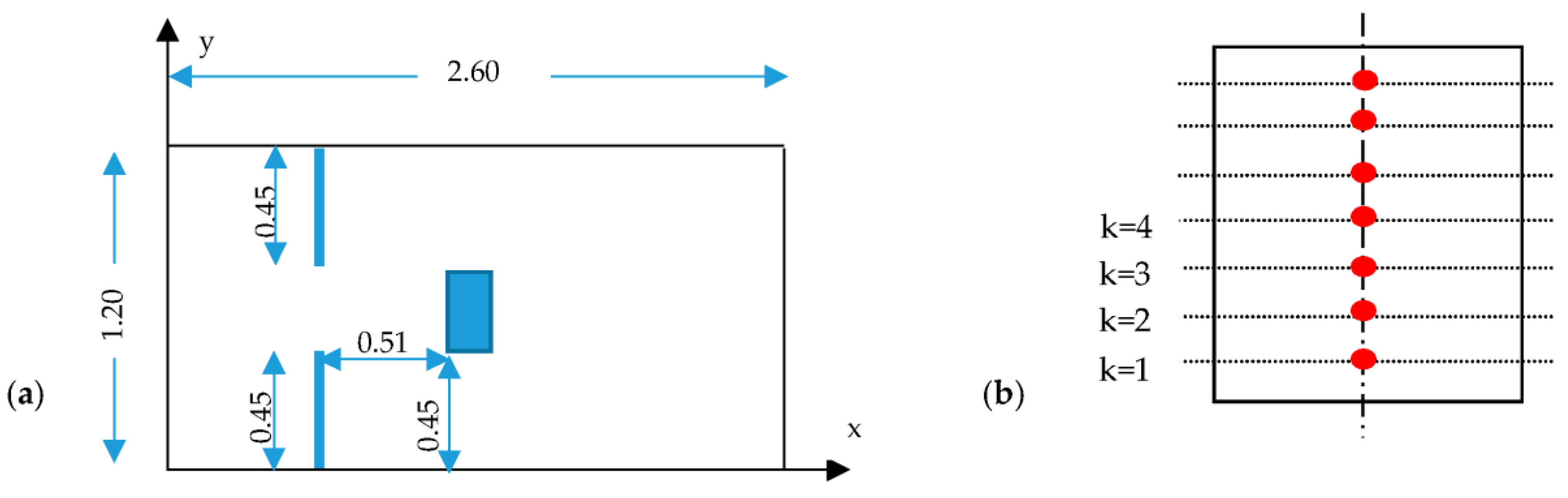
To evaluate the effect of an obstacle on a dam-break wave by numerical methods, an experiment done by Aureli [10] was used as a case study. The facility consisted of a 2.6 m long and 1.2 m wide rectangular tank divided into two compartments (Figure 1). The initial water depth in the reservoir was 0.1 m, while the floodable area was dry. To create a dam-break wave, a 0.30 m wide gauge was set up in the middle and quickly opened by a simple man-handle pulley system. A rectangle column was located at the center of the domain. Structure meshes with a cell size of 0.005 m and 0.01 m were set up in the computational domains of 2D and 3D models, respectively. The grid size of 0.005 m was also selected in the 2D numerical scheme in Aureli’s paper. The Courant number Cr was taken as 0.9. The Manning coefficient n was set equal to 0.007, and three boundaries, upstream and both sides, were closed but the downstream slip boundary was left open.

In 2D numerical solutions, with the hypothesis that the pressure was hydrostatic, the net force perpendicular to the vertical wall at each time step was estimated by applying a momentum equation to the control volume taken around the obstacle. The force per unit width (including the hydrostatic load and momentum flux term) calculated for each cell adjacent to the two walls normal to the x direction was estimated by the equation

$$f=\rho g\frac{h^2}{2}+\rho h{u}^2$$

(13)

On the other hand, the 3D numerical result of the force element acting on each cell was predicted by

$$F_{i,j,k}^n=p_{i,j,k}^n{A}_{j,k}$$

(14)

where i, j, k were indexes of the mesh cell, and n is the order of time step.

Figure 2a indicates the gauge pressure the hydrographs exerted on the center of each row from the bottom to the top of the front face of the column. Obviously, all pressure profiles had two peaks. This solution was also matched with the result of Issakhov [17]. Negative pressure was seen at some points near the top of the reflection wave. The occurrence of two pressure peaks can explain why the force solution had the same trend (see Figure 2b). Furthermore, Figure 2b presents the comparison of the total force by time simulated by the number of numerical models (2D, 3D with turbulent model RANs and 3D with the LES model). The results indicated that the 2D numerical model gave a load time history that had only one peak. The magnitude of peak force was quite close to the 3D results as well as those of the experiment data. However, the peaking time was poorly represented. It should be around 0.7 s instead of the 1.4 s shown by the experiment result, and this characteristic could be well captured by both 3D turbulent models. It was the 2D shallow-water approximation that led to the key assumption that vertical acceleration was negligible. In addition, both the magnitude and time to reach the two peaks of force predicted by the two 3D models matched well.

3.2. Force Due to Dam-Break Wave on a Group of Structures

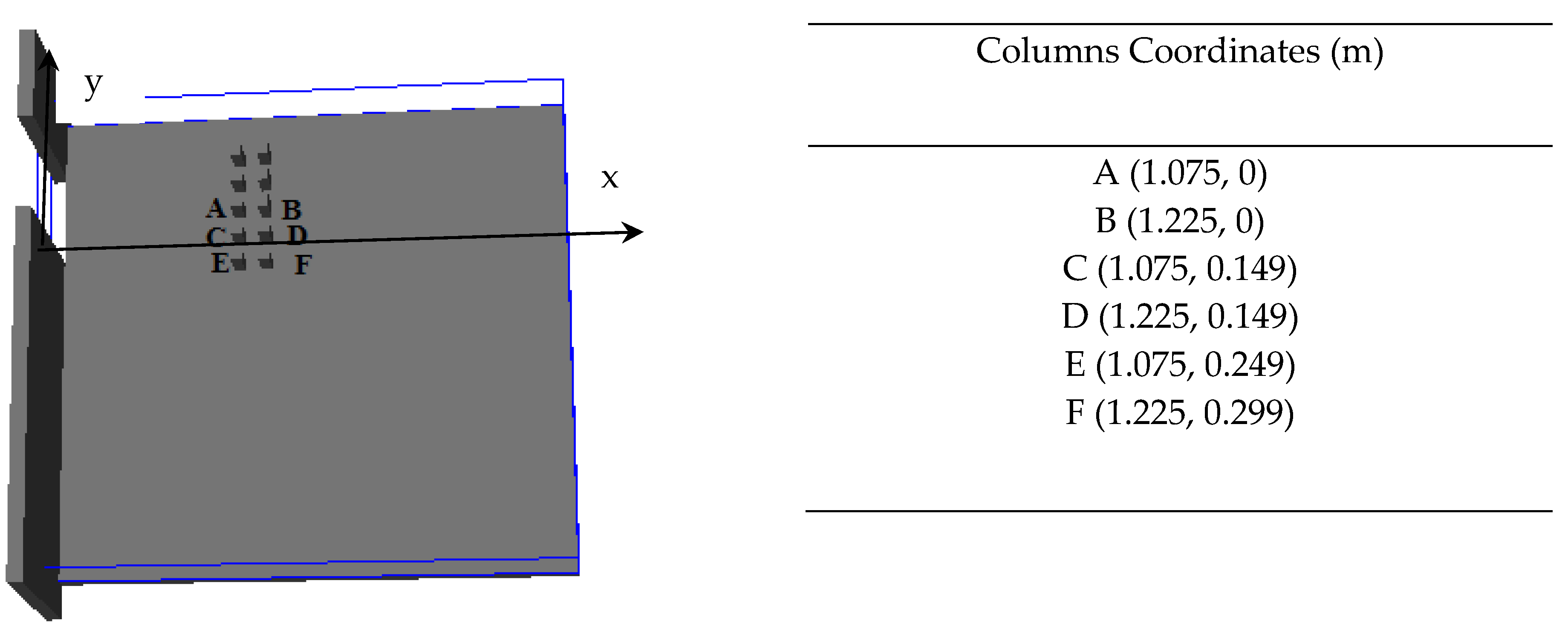
Both 2D and 3D mathematical models can represent force and other hydraulic characteristics to show how fluid flow interacts with an isolated obstruction. In the case of a group of buildings, there are few works that measure hydraulic characteristics such as water depth or velocity around the buildings [2,28]. To our knowledge, there are not many works on the observed force acting on several structures except for a case study presented in Shige-eda [12]. Therefore, this one test case in this article was reproduced in our work. The configuration of the physical model involved one reservoir with dimensions (3.0 m × 1.93 m) and a flood plain (Figure 3). The beds of both the reservoir and its downstream were horizontal and the gate was b = 0.5 m wide and located 0.75 m from the left side of the wall separating the reservoir from the flood plain. Downstream, three boundaries were opened. The initial reservoir water depth (h₀) was 0.2 m, and downstream was dry. Ten square pillars (0.06 m wide and 0.2 m high) were placed in the flood plain. The coordinates of the 6 columns which were studied are shown in Figure 3.

The observed data were provided in detail such as the water-depth profile and two components of velocity in the x and y directions at three study points a, b, c, having coordinates (0.585, 0.00 m), (0.585, 0.5 m) and (0.835, −0.75 m), respectively. Two components of the forces due to the fluid flow exerted on the 6 columns were also collected [12].

In order to obtain numerical results by the proposed 2D mathematical model, the computational domain was divided by structure mesh with Δx = Δy = 0.01 m while the original work used refinement mesh in the vicinity of the obstacles [12]. The Courant number Cr was set equal to 0.9 and the critical water depth h_e = 10⁻⁴ m was utilized to indicate whether the cell was wet or dry. The Manning coefficient n was equal to 0.007.

To simulate the propagation of a partial dam-break wave and its impact on obstacles, the flow region in Flow 3D was subdivided into rectangular cells where each cell had its own local average value of dependent variables. Two mesh blocks were set up: block 1 was inside the reservoir and had 3 wall boundaries; block 2 was in the flood plain and had 3 outflow boundaries.

a 

Mesh sensitivity analysis

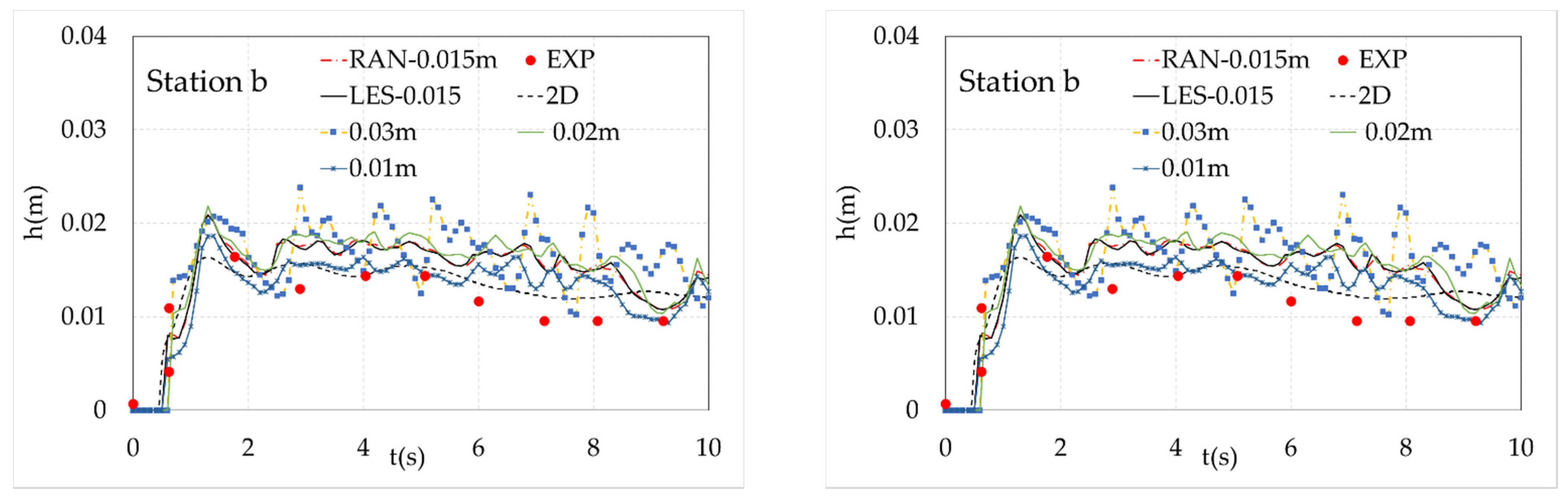
Several resolution meshes were tried out to find the best one to account for the numerical result’s accuracy and computations: 0.01 m, 0.015 m, 0.02 m and 0.03 m. Using a PC Intel^® Core ™ i5-7300HQ CPU @ 2.5GHz and an installer memory (RAM) of 8 GB, the resulting file size and computational time correspondence of 4 meshes were 87 GB, 27 GB, 12 GB, 4 GB and 9 h 17 min 28 s, 2 h 53 min 44 s, 2 h 34 min 56 s and 2 h 8 min 31 s, respectively. The cost-effective PC showed that the finest mesh generated the largest result file while the grid size of 0.015 m gave a much smaller one. Afterwards, the influence of the mesh resolutions on the accuracy of the models in predicting the flow depth (h) and velocity components (u and v) at the two study points a and b were evaluated employing the normalized root mean square error (NRMSE).

In Equation (15), X_i,exp, X_i,sim, X_exp,max and X_exp,min represented the empirical, numerical, maximum and minimum values of the X variables:

$$NRMSE=\frac{\sqrt{\frac{{\displaystyle \sum _{i=1}^n{\left(X_{i,\mathit{exp}}-X_{i,sim}\right)}^2}}{n}}}{\left(X_{\mathit{exp},\mathit{max}}-X_{\mathit{exp},\mathit{min}}\right)}$$

(15)

The NRMSE value of h, u, v at gauges a and b is indicated in

Table 1. The NRMSE value of various grid sizes and models.

Gauges	X	Grid Sizes and Models
		3D Model				2D Model
		0.01 m	0.015 m	0.02 m	0.03 m	0.01 m
a	h	0.445	0.449	0.449	0.457	0.441
	u	0.155	0.201	0.224	0.251	0.317
	v	0.277	0.277	0.294	0.407	0.454
b	h	0.264	0.345	0.438	0.619	0.697
	u	0.126	0.183	0.133	0.234	0.221
	v	0.311	0.248	0.213	0.443	0.242

.

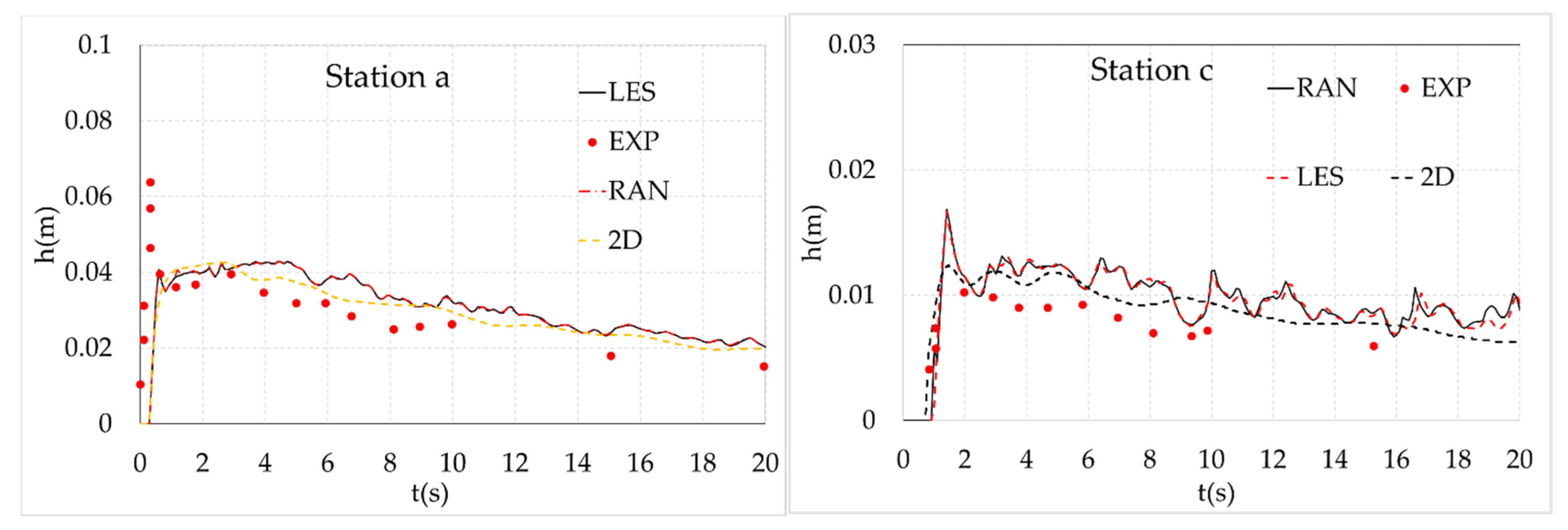
According to Table 1, the results from the finest mesh of the 3D solution showed the best agreement with the experiment data compared to other models in all gauges. The coarsest mesh size of 0.03 m gave the maximum NRMSE, which gave a very poor computed result. The 0.02 m grid gave a better result for u and v at gauge b than cell size 0.015 m while the opposite trend was seen at point a. The time series of 3D results of the coarser meshes 0.02 m and 0.03 m fluctuated strongly (Figure 4). Therefore, from the aforementioned analysis, the grid size of 0.015 m was selected to simulate the hydraulic characteristics in the 3D CFD model. Figure 5 and Figure 6 showed the numerical results of the water depth and velocity-component time series at gauges a and c according to the selected mesh size. In comparison with empirical solution taken from Shige-eda’s work, 3D and 2D results showed good agreement.

b 

Forces acting on groups of building

Shige-eda [12] used the numerical solution yielded by a 2D mathematical model in the vicinity of the flow around the columns to calculate the net force acting on each unsubmerged obstruction in the flow direction (x-axis) by the following equation:

$$D_x=F_{front,x}-F_{back,x}$$

(16)

F is the static force exerted on the front and back vertical walls of a structure. Shige-eda estimated it by the following equation

$$F_{static}={\displaystyle \sum _{}\frac{1}{2}\rho g{h}^2\times \Delta y}$$

(17)

where ρ is density of the water (ρ = 1000 kg/m³).

In the case of the 3D numerical model used to estimate this force, the formular expressed static force was

$$F_{static}={\displaystyle \sum _{}{p}_{static}\times \Delta y\times \Delta z}$$

(18)

The numerical results estimated by Equations (16) and (17) raised an argument because their magnitude was much smaller than the peak-measured force in the first impact of shock wave with obstacles. Therefore, in the discussion of this article [29], the authors admitted that in the flow direction, static pressure in Equation (18) should be replaced by dynamic pressure to account for velocity-induced pressure

$$F_{dynamic}={\displaystyle \sum _{}{p}_{total}\times \Delta y\times \Delta z}$$

(19)

where

$$p_{total}=p_{static}+\alpha \rho u^2$$

(20)

u is the velocity component in x direction; α is the parameter indicated for velocity-induced pressure (0 ≤ α ≤ 1.0).

The correct estimation of parameter α was a key phase in the design construction. Lu Liu [19] and Shige-eda [29] suggested that parameter α = 0.5.

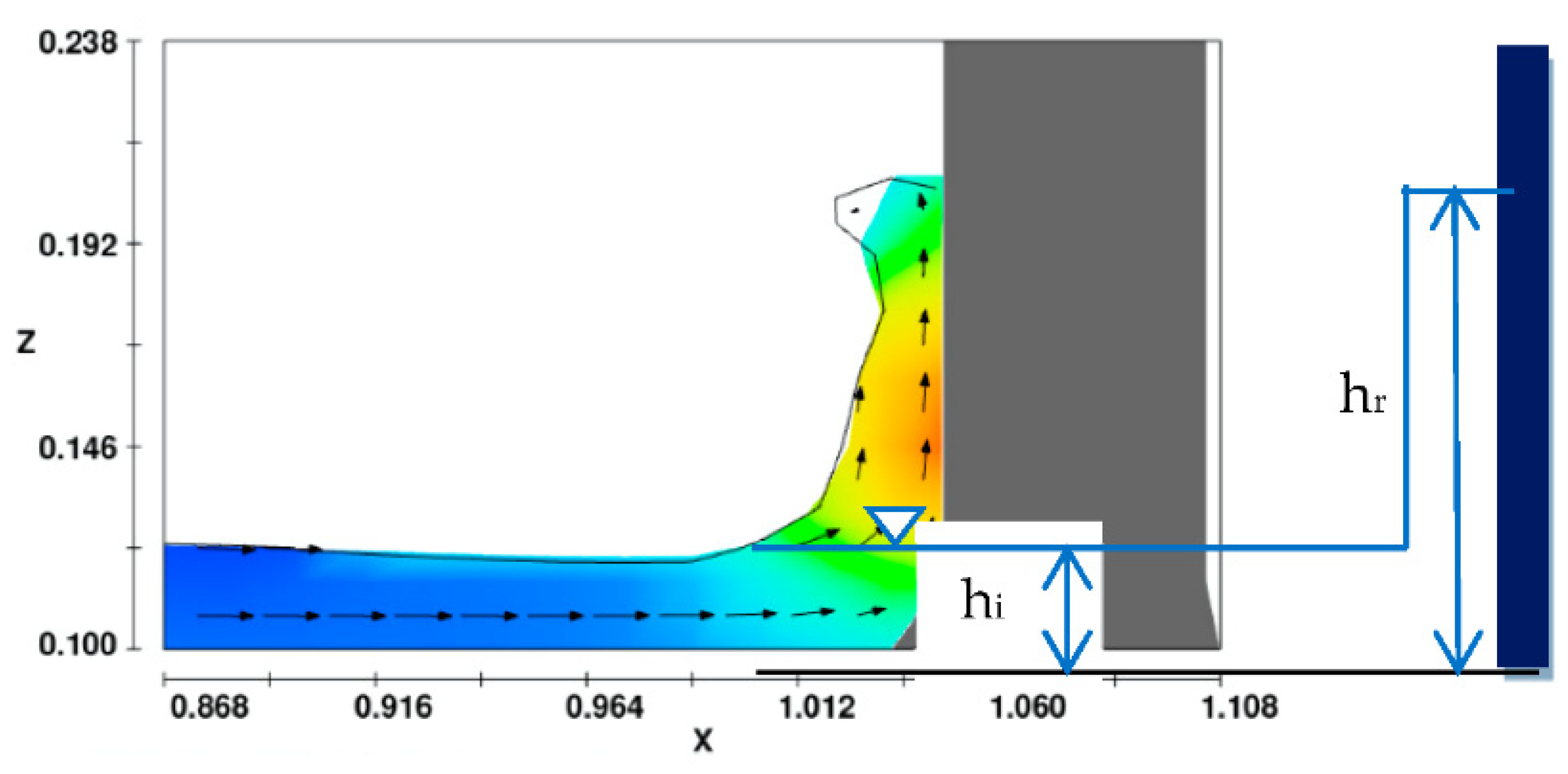
According to Armanini [20], parameter α depended on the Froude number and water depth of the incident wave. This uncertain value can be investigated using empirical data. Based on the experiment data of Shige-eda [12], the authors propose the following equation and conditions to estimate this parameter:

$$\alpha =\{\begin{array}{l}1.0\hspace{1em}if\hspace{1em}{F}_{ri}\ge 3.5 and h_i>0.01(m)\\ 0.5\hspace{1em}if\hspace{1em}3.5>F_{ri}\ge 3.0 and h_i>0.01(m)\\ 0.0\hspace{1em}if\hspace{1em}{F}_{ri}<3.0 \end{array}$$

(21)

where h_i is the depth and F_ri = u_i/(gh_i)^0.5 is the Froude number of the incident wave (Figure 7).

On the other hand, Armanini [20] suggested the following equation to estimate the impact force acting on a vertical wall based on the hypothesis of hydrostatic pressure distribution:

$$F_{steady}=0.5g\rho h_i^2\left(1+0.5F_{ri}^2\right)\left(1+\frac{\alpha F_{ri}^2}{1+0.5F_{ri}^2}\right)$$

(22)

Note that Equation (22) is suitable with steady flow. Armanini [20] also indicated the result of an impact force yielded by static phenomena was smaller than an unsteady one.

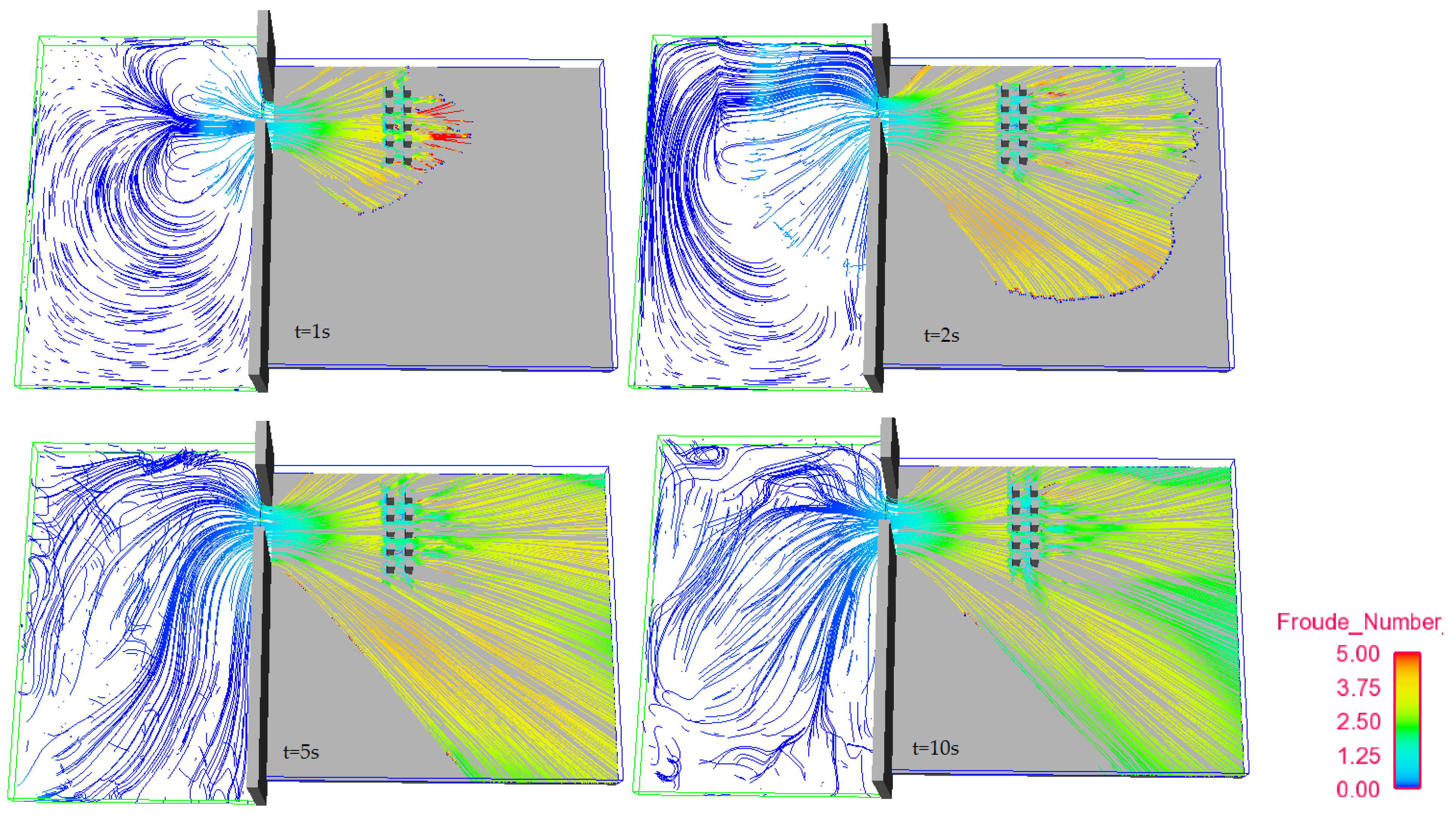
Figure 8 showed the streamline of the propagation of a dam-break wave at different times, 1.0 s, 2.0 s, 5.0 s and 10 s. In general, the streamlines in the floodable area looked like straight lines, which meant there was no significant backwater after the buildings. The direction of u velocity behind the obstruction was the same as the main flow direction, so the net dynamic force can be set equal to the difference between F_{dynamic,front} and F_static,back.

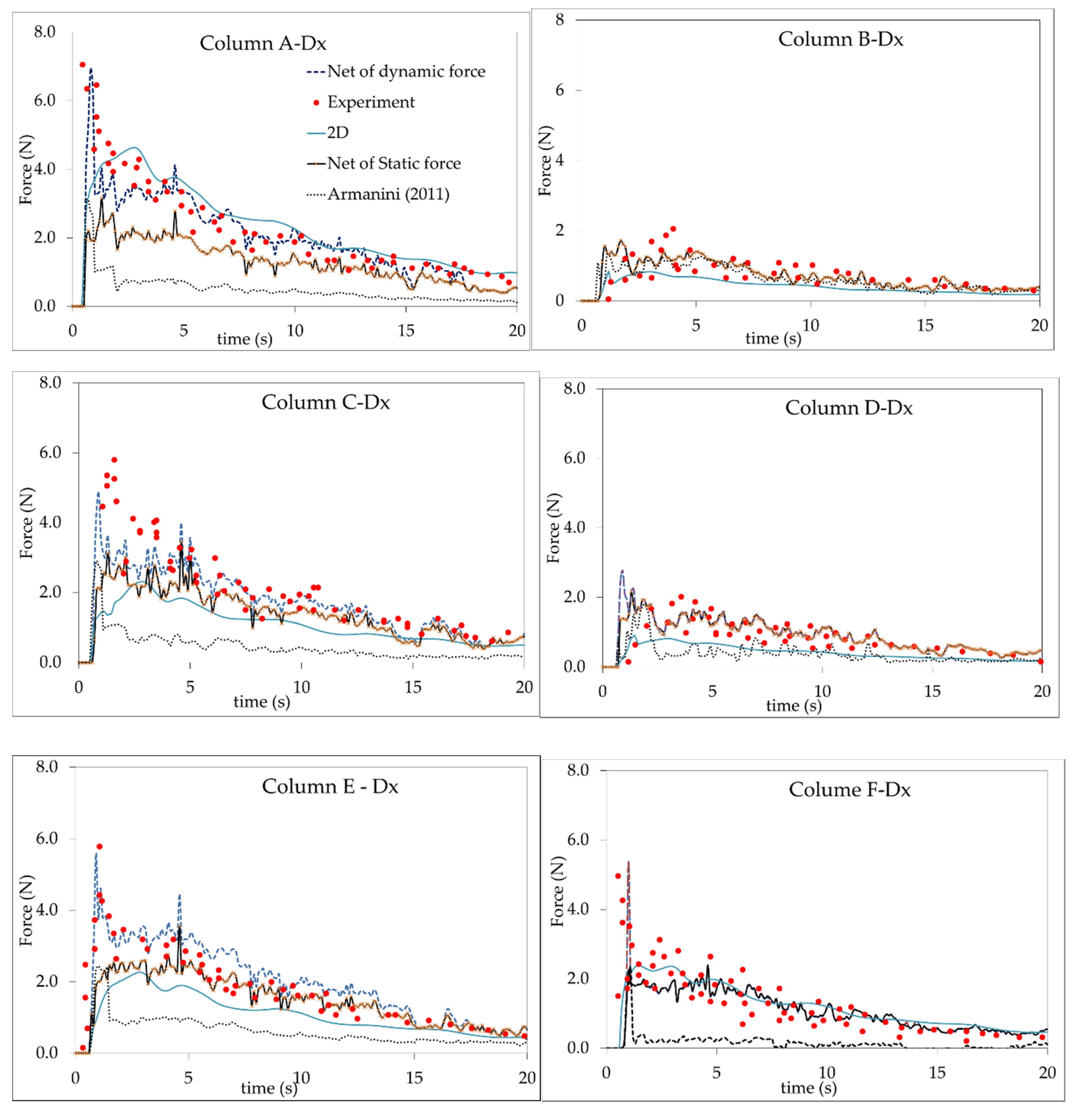
Figure 8 illustrates several results of the net force in flow direction on the 6 columns. The net static force was equal to the difference between two static forces before and after the studied building. Empirical data came from Shige-eda [12]. The net dynamic force on the buildings taken from analytical Equation (22) was also compared with other solutions.

According to Figure 9, the 3D solutions of the first peak of the dynamic force were quite close to the measured data in all 6 buildings. Meanwhile, the 3D results of the net static force became quite close to the empirical one when time increased, which means that the effect of force-induced velocity decreased over time. Furthemore, 2D solutions were underestimated in many cases. The ability of 2D shallow-water models to deal with (a) rapid surface-level changes in their vicinity and (b) dynamic pressure distribution at the water and structure or obstacle interfaces was limited. The main contribution of net force acting on all columns came from the impact load on the front sides. Therefore, from the viewpoint of safety, we should use dynamic force instead of static force when designing buildings, houses, etc. Moreover, the analytical Equation (22) was not suitable for estimating the time series of impact forces caused by the unsteady flow.

3.3. Effect of Dam-Break Width and Initial Water Level on Static Force and Dynamic Force Against Structures

In this section, the authors carried out the impact of dam-collapse width (b) as well as the initial water level (h₀) on the peak intensity of impact load generated by a discontinuous flow against the buildings using Flow 3D with the LES turbulence model.

Table 2. Case studies with different value of initial water level in reservoir and the damsite width.

Case	Initial Water Level (h0) (m)	Damsite Width (b) (m)
1	0.2	0.25
2	0.2	0.50
3	0.4	0.50
4	0.2	0.75
5	0.6	0.50
6	0.4	0.75
7	0.6	0.75

shows different scenarios.

According to Ritter’s solution [30], the unit discharge q (m³/s/m) at the damsite was estimated by the following expression:

$$q=\frac{8}{27}{h}_0\times \sqrt{g\times h_0}$$

(23)

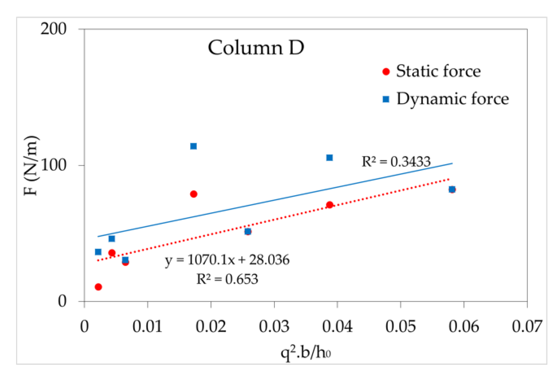
From the analysis at Section 3.2, the contribution of the static force acting on the backside of the building to the net force was much smaller than that of the front. As a consequence, we may argue that, for design purposes, evaluating the impact force on front side is a wise precaution. Two columns in the first row (A and, E) and one column in the second row (D) were selected to simulate the static force and the dynamic force exerted on the front face of three columns.

As can be seen from Figure 10, R-square quantities of linear regression between q²b/h₀ and force per unit width (F) at columns A and E were quite good (0.979 and 0.967 for static force and 0.925 and 0.853 for dynamic force, respectively). When q²b/h₀ was small, the effect of velocity-induced force was minor, so the dynamic force was close with static force. The difference between the two types of force was increased significantly when q²b/h₀ increased. Thus, dynamic force instead of static force should be estimated for design purposes in a floodplain. Column A was directly in the path of the dam-break wave propagation; hence, both its static and dynamic impact loads were the largest. Meanwhile, the location of column E was further from the path and so had smaller impact force results. On the other hand, a poor R-square value was seen at column D, which was in the second array, so the Froude number in the vicinity of this column was reduced dramatically. So, dynamic force was approximately equal to static force, and both of them were much smaller than those at columns A and E.

4. Conclusions

Flood waves due to dam-break flow have a great impact on buildings when a high velocity or a large depth is involved. In this paper, we investigated the ability of 2D and 3D numerical models to estimate the hydraulic characteristics and impact load generated by a rapid flow on a building and group of buildings. A 2D mathematical model based on shallow-water equations was solved by the FDS method, which was used together with the newest version of the Flow 3D hydrodynamic model. The main findings of the research are

(1)

To formulate water depth or velocity profiles, both 2D and 3D numerical solutions are quite similar. The proposed 2D numerical model is suitable for predicting hydraulic characteristics involving water depth and a velocity component as well as the maximum value of the static force. However, the 3D hydrodynamic model with the LES and RANs turbulent modules can well capture two peaks of impact load while the 2D shallow flow model presents only one. In general, the 3D result is closer to the experimental one.

(2)

Both the static and dynamic forces against several buildings were computed by Flow 3D with the LES module. The role of velocity-induced force and pressure force on a building varies with location. Near the damsite, the velocity-induced force is more prevalent while away from main direction of dam-break wave or in the second array the pressure force is the more important. The impact of velocity-induced force is quantified by parameter α, which is carried out as a function of the Froude number and water depth of the incident wave. The linear regression relation between q²b/h₀ and the peak intensity of the static force and dynamic force is worked out with reasonable R-square quantities.

In further study, the robustness and effectiveness of the presented 2D numerical model will be shown more clearly. It can easily be applied to simulate flood flow over large domains. Moreover, the suggested Equation (21) of parameter α will be very meaning in a real case study for evaluating exactly the influence of velocity-induced force on buildings in the downstream area. To increase the accuracy level of this parameter, several experiments of force acting on obstructions in different conditions should be implemented.

References

- Testa, G.; Zuccala, D.; Alcrudo, F.; Mulet, J.; Frazao, S.S. Flash flood flow experiment in a simplifed urban district. J. Hydraul. Res. 2007, 45, 37–44. [Google Scholar] [CrossRef]
- Soares-Frazao, S.; Zech, Y. Dam-break flow through an idealized city. J. Hydraul. Res. 2008, 46, 648–665. [Google Scholar] [CrossRef] [Green Version]
- Soares-Frazão, S.; Zech, Y. Experimental study of dam-break flow against an isolated obstacle. J. Hydraul. Res. 2007, 45, 27–36. [Google Scholar] [CrossRef]
- Soares-Frazão, S. Experiments of dam-break wave over a triangular bottom sill. J. Hydraul. Res. 2007, 45, 19–26. [Google Scholar] [CrossRef]
- di Cristo, C.; Evangelista, S.; Greco, M.; Iervolino, M.; Leopardi, A.; Vacca, A. Dam-break waves over an erodible embankment: Experiments and simulations. J. Hydraul. Res. 2018, 56, 196–210. [Google Scholar] [CrossRef]
- Evangelista, S. Experiments and numerical simulations of dike erosion due to a wave impact. Water 2015, 7, 5831–5848. [Google Scholar] [CrossRef] [Green Version]
- Li, Y.L.; Yu, C.H. Research on dam break flow induced front wave impacting a vertical wall based on the CLSVOF and level set methods. Ocean Eng. 2019, 178, 442–462. [Google Scholar] [CrossRef]
- Özgen, I.; Zhao, J.; Liang, D.; Hinkelmann, R. Urban flood modeling using shallow water equations with depth-dependent anisotropic porosity. J. Hydrol. 2016, 541, 1165–1184. [Google Scholar] [CrossRef] [Green Version]
- Mignot, E.; Li, X.; Dewals, B. Experimental modelling of urban flooding: A review. J. Hydrol. 2019, 568, 334–342. [Google Scholar] [CrossRef] [Green Version]
- Aureli, F.; Dazzi, A.; Maranzoni, A.; Mignosa, P.; Vacondio, R. Experimental and numerical evaluation of the force due to the impact of a dam break wave on a structure. Adv. Water Resour. 2015, 76, 29–42. [Google Scholar] [CrossRef]
- Milanesi, L.; Pilotti, M.; Belleri, A.; Marini, A.; Fuchs, S. Vulnerability to flash floods: A simplified structural model for masonry buldings. Water Resour. Res. 2018, 54, 7177–7197. [Google Scholar] [CrossRef]
- Shige-eda, M.; Akiyama, J. Numerical and experimental study on two dimensional flood flows with and without structures. J. Hydraul. Eng. 2003, 129, 817–821. [Google Scholar] [CrossRef]
- Cagatay, H.O.; Kocaman, S. Dam break flows during initial stage using SWE and RANs approaches. J. Hydraul. Res. 2010, 48, 603–611. [Google Scholar] [CrossRef]
- Yang, S.; Yang, W.; Qin, S.; Li, Q.; Yang, B. Numerical study on characteristics of dam break wave. Ocean Eng. 2018, 159, 358–371. [Google Scholar] [CrossRef]
- Robb., D.M.; Vasquez., J.A. Numerical simulation of dam break flows using depth averaged hydrodynamic and three dimensional CFD models. In Proceedings of the 22nd Canadian Hydrotechnical Conference, Ottawa, ON, Canada, 28–30 April 2015. [Google Scholar]
- Kocaman, S.; Evangelista, S.; Viccione, G.; Guzel, H. Experimental and Numerical analysis of 3D dam break waves in an enclosed domain with a single oriented obstacles. Environ. Sci. Proc. 2020, 2, 35. [Google Scholar] [CrossRef]
- Issakhov, A.; Zhandaulet, Y.; Nogaeva, A. Numerical simulation of dambreak flow for various forms of the obstacle by VOF method. Int. J. Multiph. Flow 2018, 109, 191–206. [Google Scholar] [CrossRef]
- Mokarani, C.; Abadie, S. Conditions for peak pressure stability in VOF simulations of dam break flow impact. J. Fluids Struct. 2016, 62, 86–103. [Google Scholar] [CrossRef]
- Liu, L.; Sun, J.; Lin, B.; Lu, L. Building performance in dam break flow—an experimental sudy. Urban Water J. 2018, 15, 251–258. [Google Scholar] [CrossRef]
- Armanini, A.; Larcher, M.; Odorizzi, M. Dynamic impact of a debris flow front against a vertical wall. In Proceedings of the 5th international conference on debris-flow hazards mitigation: Mechanics, prediction and assessment, Padua, Italy, 14–17 June 2011. [Google Scholar] [CrossRef]
- Hubbard, M.E.; Garcia Navarro, P. Flux difference splitting and the balancing of source terms and flux gradients. J. Comput. Phys. 2000, 165, 89–125. [Google Scholar] [CrossRef] [Green Version]
- Roe, P.L. A basis for upwind differencing of the two-dimensional unsteady Euler equations. In Numerical Methods in Fluids Dynamics II; Oxford University Press: Oxford, UK, 1986. [Google Scholar]
- Bradford, S.F.; Sander, B. Finite volume model for shallow water flooding of arbitrary topography. J. Hydraul. Eng. (ASCE) 2002, 128, 289–298. [Google Scholar] [CrossRef]
- Brufau, P.; Garica-Navarro, P. Two dimensional dam break flow simulation. Int. J. Numer. Meth. Fluids 2000, 33, 35–57. [Google Scholar] [CrossRef]
- Hien, L.T.T. 2D Numerical Modeling of Dam-Break Flows with Application to Case Studies in Vietnam. Ph.D. Thesis, Brescia University, Brescia, Italy, 2014. [Google Scholar]
- Hien, L.T.T.; Tomirotti, M. Numerical modeling of dam break flows over complex topography. Case studies in Vietnam. In Proceedings of the 19th IAHR-APD Congress 2014, Hanoi, Vietnam, 21–24 September 2014; ISBN 978-604-82-1383-1. [Google Scholar]
- Flow-3D, Version 12.0; User Mannual; Flow Science Inc.: Santa Fe, NM, USA, 2020.
- Guney, M.S.; Tayfur, G.; Bombar, G.; Elci, S. Distorted physical model to study sudden partial dam break flow in an urban area. J. Hydraul. Eng. 2014, 140, 05014006. [Google Scholar] [CrossRef] [Green Version]
- Shige-eda, M.; Akiyama, J. Discussion and Closure to “Numerical and experimental study on two dimensional flood flows with and without structures” by Mirei Shige-eda and Juichiro Akiyama. J. Hydraul. Eng. 2005, 131, 336–337. [Google Scholar] [CrossRef]
- Ritter, A. Die Fortpflanzung der Wasserwelle (Generation of the water wave). Z. Ver. Dtsch. Ing. 1892, 36, 947–954. [Google Scholar]
Figure 1.
(a) Configuration of experiment test (dimension in meters); (b) Gauges on the vertical front face of building.
Figure 2.
(a) Distributed pressure profiles at centerline of front face of column; (b) Comparison of load-time histories simulated by different numerical models.
Figure 3.
Group of buildings in flooded area.
Figure 4.
Water depth and u-velocity profiles at gauge b.
Figure 5.
Water hydrographs at gauges a and c.
Figure 6.
Velocity component profiles at gauges a and c.
Figure 7.
Formation of incident and reflected waves.
Figure 8.
Snapshots of streamlines of Froude number at different times: 1.0 s, 2.0 s, 5.0 s and 10 s.
Figure 9.
Force in the flow direction exerted on 6 buildings.
Figure 10.
The linear regression between forces per unit width (F) and q2b/h0.