Deterministic Model to Estimate the Energy Requirements of Pressurized Water Transport Systems


Grupo de Ingeniería y Tecnología del Agua (ITA), Department of Hydraulic Engineering and Environment, Universitat Politècnica de València, Camino de Vera s/n, 46022 Valencia, Spain
*
Author to whom correspondence should be addressed.
Water 2021, 13(3), 345; https://doi.org/10.3390/w13030345
Submission received: 5 January 2021
/
Revised: 24 January 2021
/
Accepted: 27 January 2021
/
Published: 30 January 2021
(This article belongs to the Section Urban Water Management)
Abstract
:Energy intensity, Ie (kWh/m3) is the most popular indicator when characterizing the energy requirements of the water cycle, due to its direct and easy interpretation. In pressurized water transport systems, when referred to an appropriate physical framework (such as a single water transport pipeline), it assesses the efficiency of the process. However, in complex urban water transport networks, Ie only provides a basic notion of the energy needs of the system. The aim of this paper is to define a standard physical framework for assessing the energy intensity in water transport and distribution systems. To that purpose, an analytic expression that estimates Ie is proposed, based on system data and its operating conditions. The results allow for a realistic approximation of the energy needs of water transport. This energy assessment is completed with two context indicators: energy origin (C1) and topographic energy (θt), both essential when the energy efficiency of different systems is to be compared.
1. Introduction
Efficiency is nowadays essential to maintaining the current standard of living without compromising the prospects of future generations. In a climate change context, efficiency is the key to harmonizing population growth with the rising scarcity of natural resources. The increasing commitment to circular economy aims to maximize efficiency [1]. In this context, the use of water and energy must be fully optimized. As these two resources are coupled, a joint analysis on the integral water use cycle is required. The energy intensity indicator, Ie, is relevant for this assessment, as it shows the relationship between both resources (kWh/m3) and is used to energetically characterize the whole water use cycle.
The integral water cycle can be divided in two parts. The first one (water supply) has three stages: collection–conveyance, water treatment, and distribution [2,3,4]. The second part (wastewater collection and wastewater treatment) consists of three stages: collecting, treating, and disposing of wastewater, or five, if re-use (including recycling and distribution) is included [5]. Between these two parts, water is used with significant energy requirements.
Energy intensity, Ie, has been widely used as the indicator to characterize the energy of the water use cycle from the beginning [5]. This characterization can be made for the whole water use cycle [6], for its different stages [5], on a global scale [7,8,9,10], by country [11,12], by region [5,13,14], or by city [2,15]. There are plenty of published comparisons [4,16], which can sometimes be complex due to the heterogeneity of the data. For this reason, some scholars have requested improvements in data structure and accessibility, especially in the USA [8,17,18,19,20].
In addition to energy intensity, there is a wide variety of indicators related to different aspects of energy efficiency in water transport and distribution [21,22,23,24,25]. Bylka and Mroz [26] offered an extensive review of all of them.
This article defines the framework and conditions that allow the energy intensity indicator (kWh/m3) to be used in such a way that it captures all its driving factors and reflects the energy use in water transport and distribution. Then a deterministic model is established to predict the total demand of energy. Such a model is valuable for systems at the design and operation stages. The establishment of an adequate physical framework and the cause–effect relationship of the physical system allows the energy pros and cons of the different design alternatives or layouts to be assessed. The energy efficiency of two contextual indicators can be established by comparing the actual energy intensity with the target energy intensity (resulting from the optimization of the system).
For other stages of the water use cycle, energy intensity comparisons are easier to achieve when taking context into account, as they are more homogeneous and compact. For potabilization, Ie allows the efficiency of the whole process or its individual components to be assessed: sedimentation, ultrafiltration, microfiltration, and osmosis [2,27,28]. In order to compare results, context needs to be taken into account in terms of the water source (surface, marine groundwater) and its quality [3,15,29].
In the case of desalination, the value of Ie is very sensitive to the salinity of marine water [30]. In wastewater treatment, the final quality of the effluent is a determining factor in the value of Ie [2,31,32]. Finally, concerning the efficiency of water end uses (with a well-defined framework), Ie comparisons may be reasonably conducted [29,33,34]. This is especially true with those concerning specific uses such as dishwashers, showers, etc. [29,33].
Regarding the pressurized water transport, there are three main novel contributions of this paper.
First is the establishment of what represents an adequate physical framework for pressurized water systems and the specification of the control volumes required to define the energy intensity indicator Ie. Although a trivial choice at first sight, it is only trivial in simple systems (a single pipe pumping from borehole to tank). Complex network systems present different options, some of which are not valid.
Secondly is the establishment of the biunivocal cause–effect relationship of the physical system using the integral energy equation—in other words, establishing a direct link between the physical and operational characteristics of the system (cause) and the energy intensity Ie (effect).
Last is the establishment of two context indicators to accompany the energy intensity Ie. These indicators characterize the contextual factors that may impact the energy intensity, namely, the source of energy (pumped or gravitational) and the topography of the system. These three elements in conjunction can be used to adequately compare the performance of different systems.
These three original contributions allow the current assessment method of the energy intensity in pressurized systems to be improved. Until now, systems were evaluated by dividing the pumping energy by the supplied volume, ignoring whether the system was physically meaningful and disregarding its context. As a consequence, until now it was not possible to forecast or adequately compare efficiencies in pressurized water transport (as the review of the existing models shows).
In summary, the objective of this paper is to define the framework and conditions that allow the energy intensity indicator (kWh/m3) to be used in such a way that it captures all its driving factors and reflects the energy use in water transport and distribution. Once the indicator is calculated, a deterministic model based on its value is established to predict the total demand. Such a model is valuable for systems at the design and operation stages. For the first ones, it allows the energy pros and cons of the different design alternatives or layouts to be assessed. For the latter, it allows their energy efficiency to be established, which can be calculated by comparing the actual energy intensity with the target energy intensity (resulting from the optimization of the system).
This paper is structured as follows: First, the energy intensity (Ie) calculation framework for water transport and distribution systems is established. In the following section, the driving factors for Ie are reviewed, and some of the most notable statistical regression models (developed to anticipate the energy demands of utilities) are analyzed, including their limitations. The third section presents an expression, based on the energy equation, that allows the energy intensity (and total energy consumption) of a pressurized water transport system to be anticipated, using the total water volume as an input. This expression can be used to predict the minimum energy required, based on desirable (estimated) operating values. This allows actual performance to be compared with the minimum value, and the efficiency of the process and the performance gap to be determined. Additionally, two context indicators are defined to complement this analysis: energy origin (C1) and topographic energy (θt). These two context information indicators are essential to compare the efficiency of different utilities. Finally, in order to clarify and apply all these concepts, the paper includes a real case study.
2. Fundamentals and Methods
2.1. Energy Intensity Framework
The deterministic model that predicts the energy intensity cannot be defined if the framework for its application is not previously specified. This framework allows the physical reality of the water transport and distribution network to be reduced. It is based on a system, defined as the water network contained in a control volume.
The deterministic physical model that predicts the energy intensity is based on the integral energy equation derived from the Reynolds transport theorem applied to a system that is defined by a fixed control volume [35]. In the defined system, a continuous streamline can connect any point of the system with the water sources [23], and with all existing net energy sources located outside the system. To understand this section, it is crucial to have prior knowledge of all these concepts. For instance, any booster stations in the network would not be considered part of the system, since no energy inputs should be considered inside the control volume to avoid an energy imbalance. In contrast, downstream tanks may be considered part of the system, as they are not net energy sources (when they fill up they store energy that is later returned to the system in the emptying phase).
The following examples clarify these concepts:
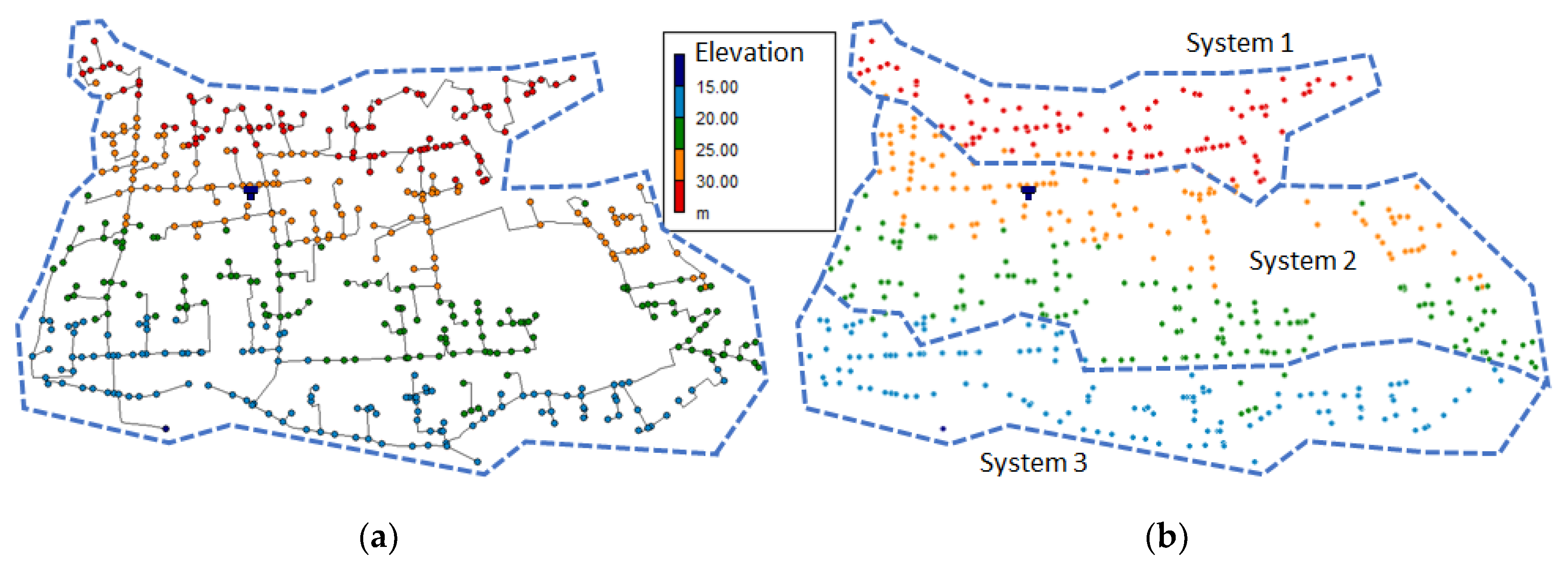
- Figure 1, shows a real pressurized network for the irrigation of agricultural plots (Cap de Terme, Spain). Each plot is represented as a node in the model. All nodes are included in the system and supplied from a pumping station (Figure 1a). Following an optimization study, it was determined that it was more energetically efficient to divide the irrigation area in three sectors based on node elevation [36]. As a result, three independent pumping stations were set up, resulting in three fully decoupled individual systems (Figure 1b).
The expression for energy intensity, Ie, has to meet two conditions. The first one is to include all the system’s physical factors that influence the value of Ie. The second condition is to be defined within a physical framework. In practice, average energy intensity is calculated as the sum of all energy consumed by pumps divided by the total registered volume. This ratio fails to capture the actual energy required by pumps, as it disregards leaks and commercial losses which would make the denominator larger.
However, in practice the water transport and distribution of a utility is integrated by several systems. Therefore, its global efficiency should be calculated as the average of all individual system efficiencies, weighted by volume and considering the gravitational energy. In any case, a sectorial efficiency analysis (by system) holds more interest than the global average, as it allows improvement actions for each sector to be prioritized (similar to studying water efficiencies by sectors or for the whole network).
The existing reported calculations of the Ie indicator correspond to pumping in single pipes, with a reference value of 0.4 kWh/m3 for 100 m of elevation [39]. These systems comply with the framework conditions previously established, as they are physical systems without discontinuities or unbalanced energy inputs, regardless of the pumping station’s location. However, in order to expand the application of this indicator to more complex distribution networks, and as explained previously, networks have to be subdivided in systems and consider gravitational energy.
2.2. Factors Influencing a System’s Energy Needs
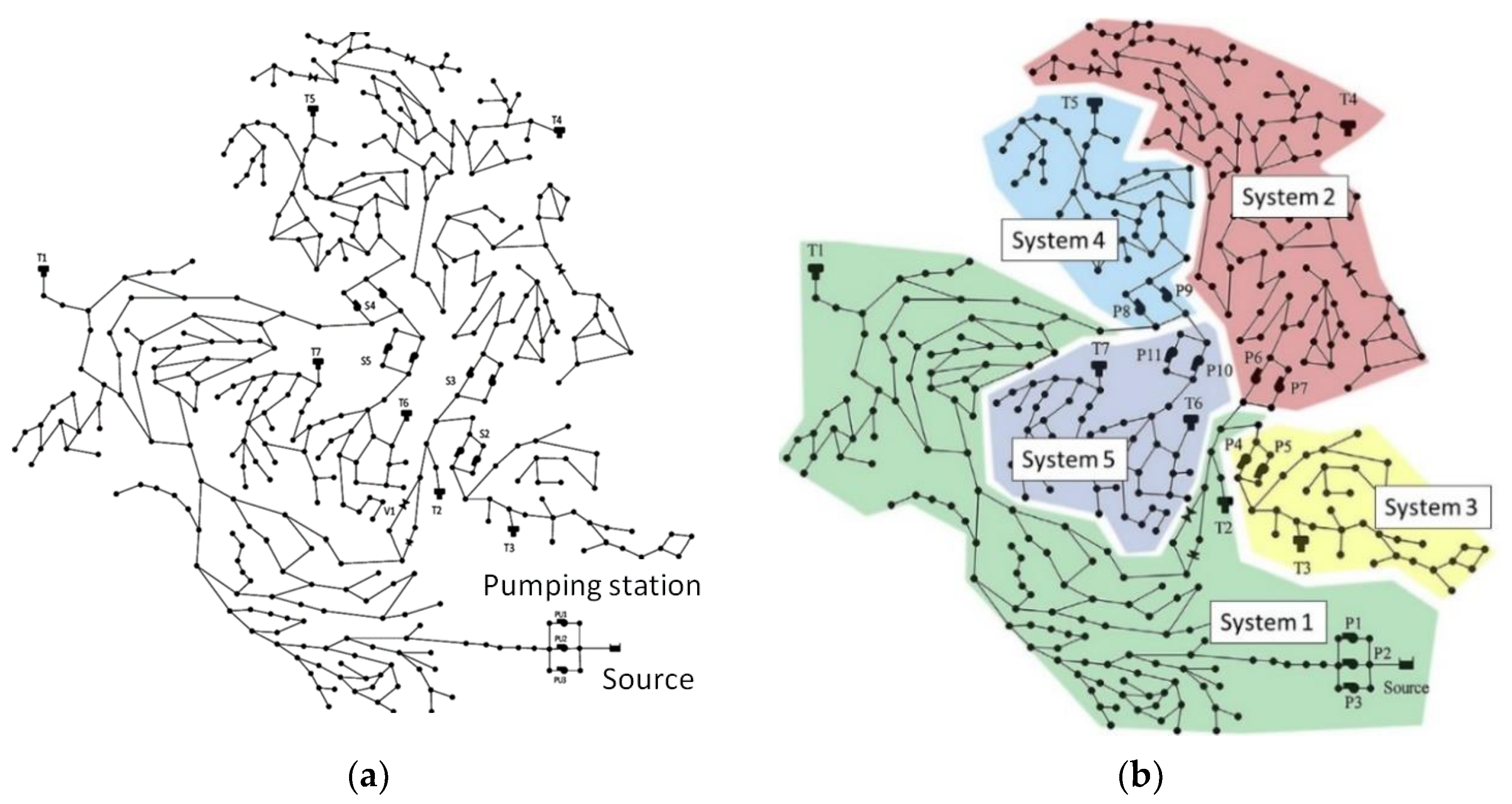
Once the framework for the application of the energy intensity indicator has been defined, the factors that influence energy use need to be identified. Only when the analytical expression that estimates energy use takes all these factors into account is this expression universal. This is why the validity of the three regression models explained below is limited to their specific framework of application, as they ignore several factors that affect the energy requirements (e.g., in Figure 3, the model considers a single system instead of disaggregating it in five systems, as suggested by the framework presented in the previous section). All these models are based on data from groups of utilities with similar geographical environments to identify the key energy-related parameters. Afterwards, the coefficients of the model are used to adjust the importance of each factor by means of their weight.
The first explained predictive model for annual energy consumption [2] is based on the statistical analysis of 86 utilities in the USA. The authors concluded that the model reaches a good fit, taking into account six variables: average daily total flow, purchased daily flow, total pump horsepower, raw/source pump horsepower, change in distribution elevation, and total water main length. Nevertheless, the subsequent analysis by the authors uncovered some weaknesses in the model. These weaknesses are related to two absent factors (water losses and friction) and the omission of natural energy. In their conclusions, the authors pointed out that these limitations could impact the validity of the proposed model.
The second statistical model [6] is based on data from 108 USA utilities. The authors identified the five variables with the greatest impact on energy consumption. Two of them coincide with the previous model: annual water use and imported water supply. The additional variables are gravity-fed water supply, average annual rainfall, and average annual temperature. These last two variables affect water demand and, indirectly, have an impact on energy.
Both these models include the potabilization phase, although (as the authors concluded), the energy associated with this process is small compared to the energy used in transport.
In the third model, proposed by Sanjuan-Delmás [40], the energy consumption is based on energy intensity. Using data from 50 medium-sized Spanish utilities, the model identifies the three variables with the greatest impact on energy consumption: metered water, network length, and number of inhabitants. However, some key variables are ignored, as indicated by the authors in the text. Once again, the homogeneity of the sample allows the validation of a clearly local model. This is the reason why the qualitative analyses of different countries only provide an order of magnitude [41].
Summing up, the avoidance of the key driving factors for energy consumption leads to local models (with a homogeneity in factors). A model is universal and deterministic when it includes within the physical system boundaries all energy consumption factors, even though some of them may turn out to be irrelevant for some systems. Otherwise it can produce inconsistent results [42].
It is consequently fundamental to identify those driving factors. In this work, up to eight key factors for energy consumption were identified: three linked to physical system characteristics, two dependent on service conditions (pressure and volume), and three factors affected by operational inefficiencies.
Factors dependent on physical characteristics of the system include:
- Topography, summarized in three elevation figures: the elevation of the network’s lowest node (which sets the reference level), the elevation of the most energy-demanding node (as explained later, in a few cases it is not the same as the highest node), and the source’s elevation;
- The distances traveled by water;
- The natural energy supplied to the system;Factors linked to service conditions;
- The pressure values at the supply sources (usually zero) and at the delivery nodes (dependent on use), where any excess of pressure over the required value leads to energy loss; and
- The water volume injected to the system Vt, the spatial distribution of water delivered to users (with the corresponding elevations), and the total metered volume Vr;
Finally, the three factors affected by operational inefficiencies are:
- Pumping efficiency;
- Leakage; and
- Friction losses.
These energy losses depend to a large extent on the operation of the system; pressure needs to be managed and pumps should operate at their BEP (best efficient point). However, they also depend on system design (selection of pumps, diameters, and pipe materials) and assembly (leaks are very sensitive to pipe assembly). The only inefficiencies not included in these factors are the structural inefficiencies, represented by the topographic energy indicator (θt) [36].
The energy intensity predictive model proposed in the following section includes these eight factors and allows for the prediction of, following a top-down approach, the energy consumed under estimated operation conditions once the metered water volume is known. The comparison with the actual consumed energy, calculated in a bottom-up path (actual energy consumption vs. billed volume), yields the current efficiency of the system. This comparison should be carried out with care, since the predictive value includes all forms of energy (natural and pumped), whereas the real value (usually) only considers pumped energy, and not the gravitational one. Only energy intensities obtained with the same conceptual framework should be compared.
As a result from the previous considerations, we can define four values of energy intensity:
- Analytically estimated values (top-down): estimated energy intensity (Iee), including all the supplied energy (natural and pumped), or the estimated pump energy intensity (Iee,p), only considering mechanical or shaft energy; and
- Real values (bottom-up), calculated from real operating data: real energy intensity (Ier), including all supplied energy (Es), and the real pump energy intensity (Ier,p), which only accounts for shaft energy (Ep).
These energy intensity values should be compared in pairs as follows: Ier with Iee or Ier,p with Iee,p. In general, the second pair is used more often, as the required data is easier to obtain by utilities.
2.3. Deterministic Model for the Prediction of the Energy Demand of a System
In order to develop the model, the Iee and Iee,p values are obtained analytically (top-down approach). This section describes the deterministic predictive model for single-source systems. This model is later generalized to consider the case of multi-source systems.
Using physical and operational data from the system, Equation (1) allows the energy behavior of the network to be predicted. This equation was obtained in a previous work [39]. The equation includes all the factors driving energy demand detailed in the previous section and, as a consequence, properly reflects the energy requirements of the process. However, it is not the only indicator linked to the energy efficiency of pressurized water transport.
In order to enable a direct comparison, Iee and Iee,p need to be referred to the metered water volume (Vr), as this is the volume used by utilities to calculate the real energy intensity (Ier = Es/Vr and Ier,p = Ep/Vr). Vr is, by definition, lower than the input volume (Vt), and they are both included in Equation (1) through the water efficiency ratio of both volumes (ηle = Vr/Vt). Energy terms are divided into gravitational energy availability (not impacted by the pumping efficiency, ηpe) and shaft energy requirements. In consequence, greater inefficiencies (ηle and ηpe) lead to worse values for Iee.
The remaining terms of Equation (1) are:
- 0.002725, a unit conversion factor (pressure, expressed in m, to kWh/m3);
- zs, elevation of the supply source;
- zl, lowest elevation node;
- zc, elevation of the node with the highest energy demand, also known as the critical node (it should be noted that zc is not necessarily the same as the highest node, zh, as friction losses also play a role and difference in elevation could be compensated by additional distance from the source);
- hfe, friction losses from the source to the critical node = ;
- friction losses from the source to the pumping station;
- friction losses from the pumping station to the critical node;
- po, service pressure; and
- γ: specific weight for water (9810 N/m3).
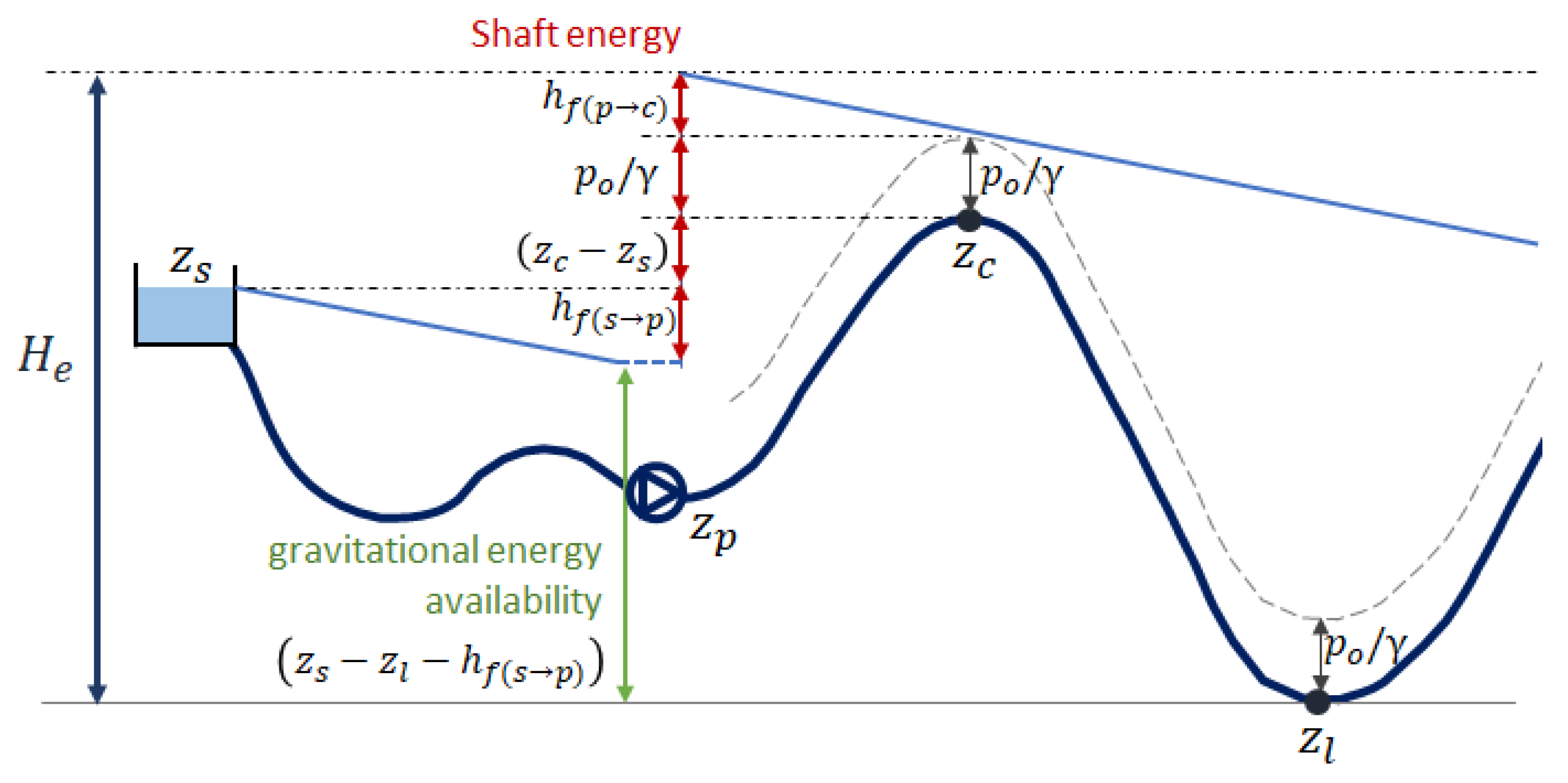
Figure 4 illustrates the preceding defined variables in a pumping booster system. It can be treated as a control volume because there are no nodes between the source and the pumping station.
On the other hand, gravitational systems were usually left out of previous studies because they lack pumping stations. However, they are reviewed in the next section to guarantee the universality of the indicator.
Synthesizing Equation (1), the estimated system’s maximum piezometric head, , (Figure 4) can be defined as:
Thus simplifying the form of the estimated energy intensity:
Finally, the critical node is the one that fulfills the relationship:
where is the elevation of a generic node i, is its piezometric head, is the maximum piezometric head, and is the piezometric head of the critical node; represents friction losses between the pumping station and the generic node i.
The result of Equation (1) is conditioned by the critical node. The equation allows for the estimation of the energy required by the system to supply water to the critical node with the pre-set service conditions. Since all nodes are interconnected (they are part of a system), they all receive identical energy from the source of supply, but part of that energy is lost in the path from the source to each node due to friction.
In addition, part of the supplied energy ( is not strictly necessary in most nodes, but it must be supplied due to the irregularities of the terrain. So strictly speaking, there is an excess energy supplied to nodes; the topographic energy (Et) and its relative importance is provided by the topographic energy context indicator θt [43]:
where is the weighted average elevation of the system. The critical node should not have any topographic energy, as it should receive just enough energy to meet the quality-of-service standards. This indicator is key to comparing the energy intensity between different utilities, as it considers the structural inefficiencies due to the irregularities of the terrain [36].
The second context indicator is the energy origin (C1) indicator. This ratio specifies which percentage of the total supplied energy corresponds to natural or gravitational energy (En):
where En is the natural or gravitational energy, Ep is the pumped energy, and Es is the total supplied energy, calculated as the sum of the previous two. Should all supplied energy be gravitational, C1 would be equal to 1, and if all the energy were provided by pumps, its value would be 0. Natural energy has traditionally not been taken into account in energy analyses, and for instance EPANET does not consider it in its energy calculations [44]. However, this energy must be considered when comparing the energy efficiency of different utilities.
The estimated pump energy intensity (Iee,p) is a relevant indicator, as it is a benchmark for the real energy intensity (Ier,p) traditionally calculated by utilities. These two indicators do not include natural energy. Therefore, Iee,p is identical to Iee (Equation (1)) if the contribution of the natural energy is excluded:
Both estimated energy intensities are linked through the context indicator C1 (energy origin):
From the estimated energy intensities (Iee and Iee,p), both the total energy ( and shaft energy needed for a registered water volume Vr can be anticipated, based on the estimated working conditions (values of and ):
These two equations conform to the deterministic model that, relating cause and effect, allows the energy consumption due to transport in a system to be estimated. This energy consumption depends, to a greater or lesser extent, on the eight factors listed previously.
Both equations involve the metered water volume Vr, to which the energy intensities have been referred. This volume can be easily converted to the total input water volume (Vt) by deleting the term in the denominators of Equations (1), (2), (6) and (7).
Finally, the temporal variation of the top-down estimated indicators is worth consideration. Depending on the load of the network, the critical node may change, as friction losses are not constant. These changes impact the values of Iee and Iee,p. However, the real indicators to which they must be compared (Ier and Ier,p), are usually averaged values referring to extended periods of time (days, months, or even years). Therefore, it does not make sense to consider hourly variations of the estimated indicators, even though the proposed mathematical formulation allows for it. The weighted average should be calculated for the same period of time to allow for comparison with the real indicator. Consequently, average values of time-dependent variables (e.g., tank water levels) extended over the selected period must be considered.
2.4. Generalization of the Model to Other Systems
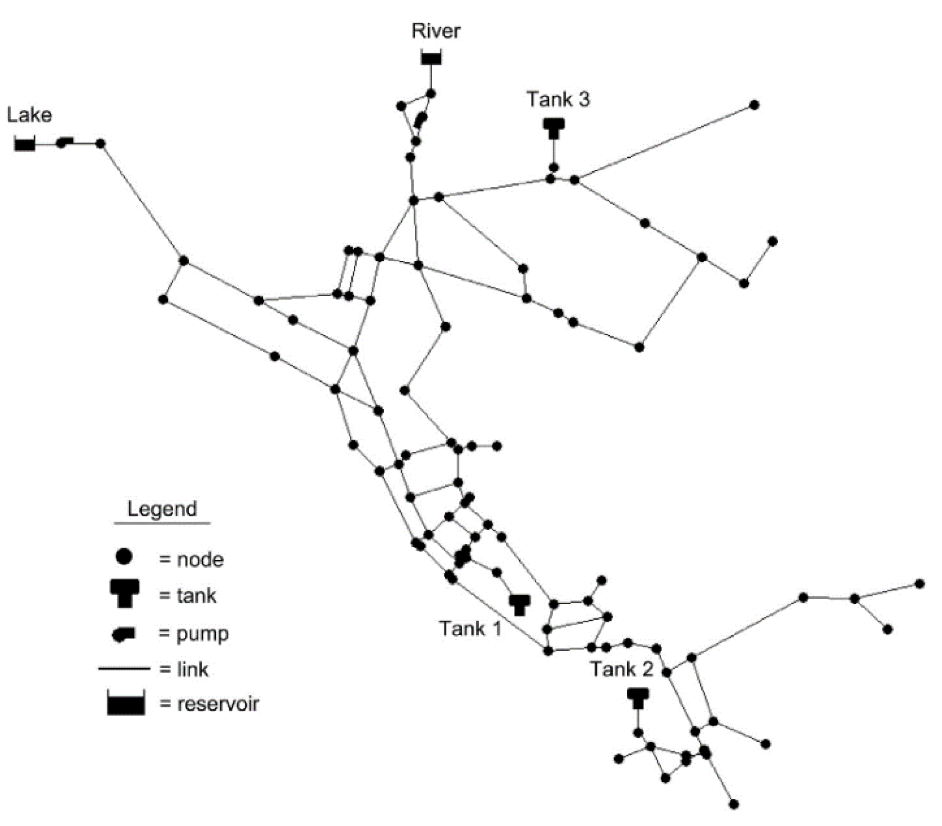
This section generalizes the previous equations to gravitational systems and those with more than one supply source (Figure 2). In gravitational systems, the source of supply is the highest node and the inequality zs = zh > zc is met, with two possible cases:
- The difference in elevation between the source and the critical node is lower than the friction losses plus the service pressure:where is the friction losses between the source and the critical node. In this case, additional pumping energy is needed to satisfy the energy demand of the gravitational system. This situation is similar to the previous one analyzed, modeled by Equation (1).
- The difference in elevation between the source and the critical node is equal to or greater than the friction losses plus the service pressure:
In this case, the energy intensity is
The water efficiency () included in the equation factors in the influence of leaks and penalizes the result accordingly, as the metered water volume does not consider them.
Obviously, all the preceding considerations for systems with zc > zs, considered in Equations (2) to (10) are also valid for gravitational systems.
All these concepts should also be extended to multi-source systems, where in general zc is higher than any of the supply sources (there are as many zsi as supply sources). However, being part of a system, the elevations of zc and zl are unique. Since pumping efficiencies of the pumping stations can be different, an average pumping efficiency () weighted by volume can be used.
Despite the singularities of a multi-source system, the same framework can be applied. In order to calculate the energy intensity, the first step is to identify the source with a higher contribution in unit energy (the one with higher piezometric head at the exit). Then the critical node of the system must be identified with Equation (4) adapted to a multi-source system:
In this case, is the piezometric head of the highest source of supply and represents the friction losses between this source and the generic node i.
Then the energy intensity injected by each supply source (may have different piezometric heads) is weighted with the corresponding volume. The estimated energy intensity is
where is the elevation of the source with a higher piezometric head, is the input volume from source i, is the piezometric head of source i, is the total supplied volume, and k is the number of supply sources in the system. The new equivalent head, He, is
The energy origin (C1) context indicator needs to consider that the natural energy contribution from each source is different, resulting in Equation (6) being expressed as
where is the weighted average elevation of the supply sources.
The topographic energy indicator, Equation (5), is not affected by the number of sources. Once the multi-source system has been characterized, the final Equations (9) and (10) that synthetize the model are the same.
The validity of the multi-source equations was tested by analyzing the system in Figure 2. The real energy required by the model was calculated from the mathematical model that simulates the operation of the network. This result was compared to those obtained with Equation (9), particularized for a system with two sources of supply.
It has to be noted that in this example, the critical node changes with time, as does the energy intensity. In particular, when the downstream tanks are being filled up, the one with the highest level is the critical node. As the tanks are being emptied, the highest consumption node becomes the critical node. This network has greater friction losses than recommended (more than 10 m/km during peak periods [45]). As a result, the energy intensity changes significantly with time, making this network especially adequate for validating Equation (12).
In this example, the validity of the analytical expressions corresponding to a multi-source network were verified with a mathematical model that faithfully reproduces the behavior of the real system. In a real network, a mathematical model is not required, since all variables can be measured.
Finally, in order to complete all possible scenarios, a possibility exists for a multi-source system where some or all of the sources are higher than the critical node (multi-source gravitational systems). In this case, the energy intensity would still be calculated from the established guidelines, requiring a good understanding of the physics behind these equations. In any case, these systems are, in practice, often overlooked, as they do not include relevant pumping stations, if at all.
3. Application of the Model to a Real Case. Results and Discussion
The framework presented in the previous sections was applied to a sector (Cansalades, Figure 5) of the water supply network of the city of Jávea (Spain). Jávea has a complex topography, with 650 km of mains, 10,000 connections, about 20 booster pumping stations, and a similar number of downstream tanks. The network is similar in nature, although on a bigger scale, to the C-Town network presented in Figure 3.
The sector of Cansalades is a representative sector of Jávea. Its supply source (a water storage tank) has an elevation of 84 m, from which a pumping station supplies all the sector. The presented simulation, performed with EPANET, corresponds to one month of operation. This is a dynamic real system with variable demands over time, and the indicators that assess its energy performance are also variable. Consequently, in order to obtain a meaningful diagnostic, the energy balance has to be referred to an extended and significant period of time. In our case, this was one month.
The physical characteristics of the sector are:
- Length = 45.1 km;
- Critical node elevation (in this case, it coincides with the highest node) zc = 120.66 m;
- Pump suction head zs = 84.00 m;
- Elevation of the lowest node zl = 35.64 m;
- Distance between the source and the critical node = 4.5 km;
- Minimum service pressure po/γ = 20 m; and
- m (pumping station next to tank).
Operational data:
- Input water volume Vt = 15,386 m3/month;
- Metered water volume Vr= 8994 m3/month;
- Real water efficiency (includes real and apparent losses) ηlr = 0.58;
- Energy consumed by the pumping station = 3902.25 kWh/ month;
- Average pumping efficiency, ηpr = 0.70; and
- Friction losses were estimated at 1.4 m/km [45], resulting in an estimated friction hfe of 6.3 m.
The example was structured as follows: In the first place, the energy intensity was estimated following a top-down approach (Iee and Iee,p). Then the predictive capacity of the model was checked by comparing the estimated values with the real ones (Ier e Ier,p), obtained through a bottom-up approach.
The calculation of the real values Ier and Ier,p is straightforward:
To calculate the real energy intensity (, it is first necessary to determine the natural energy of the system, En:
Hence:
A comparison between the estimated (Iee = 0.64 kWh/m3) and real values (Ier = 0.66 kWh/m3) concludes that the predictive model is quite accurate.
Additionally, the energy origin indicator provides information about the main energy source (natural or pumped). This information is relevant to analyzing results and proposing energy efficiency improvements:
This result indicates than the 34% of the supplied energy is natural. The main source of energy supply in this case is the pumping station.
After analyzing the energetic efficiency of the sector, potential improvements were considered. To this end, the potential gains in energy intensity achievable by improving water losses and pumping efficiency were estimated. Target values adequate to urban water networks of these characteristics were set: ηpe = 0.75 (the EPANET reference value [37]) and ηle = 0.80 (the minimum value adopted by the Portuguese regulator for good leakage management [46]). With these target values, the energy intensity achievable in this sector would be
By comparing the estimated values (Iee,p = 0.29 kWh/m3) with the real values (Ier,p = 0.43 kWh/m3), the improvement margin at the pumping station (Ier,p − Iee,p) would be 0.14 kWh/m3. These unit energy savings are achievable by improving the water losses and pumping efficiencies.
The previous analysis does not include the spatial distribution of water demand. As a consequence, the structural water losses weight cannot be determined. Their relevance can be assessed with the topographic context indicator θt, which can be evaluated with the average elevation (weighed) of the network. In this case, it was 67.7 m.
Consequently, the topographic energy would be quite significant in this example, being half of the supplied energy. This would suggest improvements such as layout changes, installation of PATs (pumps as turbines) or turbines (a solution nowadays widely explored, because it is of great interest to recovering topographic energy [47]), or energy dissipation through valves. The authors covered the issue of structural losses in previous studies [36,48].
4. Conclusions
The energy intensity indicator is, by far, the most popular for characterizing the energetic needs of the different stages of the integral water cycle. However, in order to use it for comparative performance assessment, the indicator needs to be applied to a coherent physical framework and include all supplied energy (natural and pumped). These two requirements are met in almost all the stages of the integral water cycle, and yet many of the analyses carried out in the transport phase for pressurized networks do not consider them [49]. Other studies, such as those dealing with single pipe pumping facilities, do fulfil these requirements, and as a consequence the obtained energy intensity (about 0.4 kWh/m3 for every 100 m of pumped head) are a representative measure of their efficiency. As a result, the statistical regression models that were presented to estimate the energy needs of transport in a utility are quite local in nature and have limited validity.
This paper presents a predictive and general model to estimate the required energy intensity. It uses a top-down approach that is applicable in a coherent physical framework, relating the causes (physical characteristics and operation of the system) with the effects. This is a relevant result, for it allows the energy needs for a system to be forecast based on its operating conditions, and additionally, the efficiency of the process to be diagnosed (by simple comparison of estimation and reality).
The proposed energy intensity indicator Iee includes all factors that have an impact on the total energy consumption. Additionally, two context indicators are recommended to provide key information when comparisons between utilities are to be made. The first one, C1, details the origin of the energy (natural or pumped). The second, θt, indicates the weight of the topographic energy (structural energy losses). The management of these losses by their reduction (modification of the layout), recovery (installing PATs), or remove (with pressure reduction valves), the three R, is beyond the scope of this work.
The energy efficiency measurement framework proposed in this work allows for the standardization of the calculation of the energy intensity. Its analysis, together with the two proposed context indicators, allows for a comparison of energy efficiency of different utilities, and its use by water regulatory authorities.
Author Contributions
Conceptualization, E.C.; methodology, E.C., R.d.T. and E.G.; software, E.G.; validation, E.G. and E.E.-J.; formal analysis, E.G.; investigation, E.C. and E.C.J.; resources, E.C.J.; data curation, E.G.; writing—original draft preparation, E.C.; writing—review and editing, R.d.T., E.C.J. and E.E.-J.; visualization, R.d.T. and E.E.-J.; supervision, E.C.; project administration, R.d.T. All authors have read and agreed to the published version of the manuscript.
Funding
This research received no external funding.
Institutional Review Board Statement
Not applicable.
Informed Consent Statement
Not applicable.
Conflicts of Interest
The authors declare no conflict of interest.
Nomenclature
| Symbols | Meaning of Symbols |
| C1 | Energy origin context indicator (kW h) |
| Es | Supplied (or injected) energy (kW h) |
| Ese | Estimated supplied energy (kW h) |
| En | Natural or gravitational energy (kW h) |
| Ep | Shaft (pumping) energy (kW h) |
| Epe | Estimated shaft energy (kW h) |
| Et | Topographic energy (kW h) |
| Hc | Piezometric head of the critical node (m) |
| He | Estimated maximum piezometric head of the system (m) |
| Hi | Piezometric head of a generic node i (m) |
| Hs | Piezometric head of source (m) |
| Hs,i | Piezometric head of source i (m) |
| Elevation of the highest source of supply | |
| hfe | Friction losses from the source to the critical node (m) |
| Friction losses between the source and the generic node i (m) | |
| Friction losses between the source and the critical node (m) | |
| Friction losses between the highest source and the generic node i (m) | |
| Ie | Energy intensity (kW h m−3) |
| Iee | Estimated energy intensity (kW h m−3) |
| Iee,p | Estimated pump energy intensity (kW h m−3) |
| Ier | Real energy intensity (m km−1) |
| Ier,p | Real pump energy intensity (m km−1) |
| k | Number of supply sources in the system |
| po | Service pressure (N m−2) |
| Vr | Metered water volume (m3) |
| Vt | Total input water volume (m3) |
| Vi | Input volume from source i (m3) |
| VT | Total supplied volume (m3) |
| Weighted average elevation of the system (m) | |
| zc | Elevation of the node with the highest energy demand (m) |
| zh | Elevation of the highest node (m) |
| zi | Elevation of a generic node i (m) |
| zs | Elevation of the supply source (m) |
| zs,max | Elevation of the source with a higher piezometric head (m) |
| zl | Elevation of the lowest node (m) |
| Weighted average elevation of the supply sources (m) | |
| γ | Specific weight of water (N m−3) |
| ηle | Estimated water efficiency |
| ηpe | Estimated pumping efficiency |
| Average estimated pumping efficiency | |
| θt | Topographic energy context indicator |
References
- Stahel, W.R. Circular economy. Nature 2016, 531, 435–438. [Google Scholar] [CrossRef] [PubMed] [Green Version]
- Carlson, S.W.; Walburger, A. Energy Index Development for Benchmarking Water and Wastewater Utilities; AWWA Research Foundation: Denver, CO, USA, 2007. [Google Scholar]
- Plappally, A.K.; Lienhard, J.H. Energy requirements for water production, treatment, end use, reclamation, and disposal. Renew. Sustain. Energy Rev. 2012, 16, 4818–4848. [Google Scholar] [CrossRef]
- Wakeel, M.; Chen, B.; Hayat, T.; Alsaedi, A.; Ahmad, A. Energy consumption for water use cycles in different countries: A review. Appl. Energy 2016, 178, 868–885. [Google Scholar] [CrossRef]
- Klein, G.; Krebs, M.; Hall, V.; O’Brien, T.; Blevins, B. California’s Water–Energy Relationship. Final Staff Report; California Energy Commission: Sacramento, CA, USA, 2015.
- Sowby, R.B. New Techniques to Analyze Energy Use and Inform Sustainable Planning, Design, and Operation of Public Water Systems. Ph.D. Thesis, University of Utah, Salt Lake City, UT, USA, 2018. [Google Scholar]
- Vilanova, M.R.N.; Balestieri, J.A.P. Energy and hydraulic efficiency in conventional water supply systems. Renew. Sustain. Energy Rev. 2014, 30, 701–714. [Google Scholar] [CrossRef]
- Sowby, R.B.; Burian, S.J.; Chini, C.M.; Stillwell, A.S. Data Challenges and Solutions in Energy-for-Water: Experience from Two Recent Studies. J. Awwa 2019, 112, 28–33. [Google Scholar] [CrossRef]
- Liu, F.; Ouedraogo, A.; Manghee, S.; Danilenko, A. A Primer on Energy Efficiency for Municipal Water and Wastewater Utilities; Technical Report 001/12; The International Bank for Reconstruction and Development: Washington, DC, USA, 2012. [Google Scholar]
- Lee, M.; Kellerb, A.A.; Chianga, P.C.; Denc, W.; Wangd, H.; Houa, C.H.; Wue, J.; Wange, X.; Yane, J. Water-energy nexus for urban water systems: A comparative review on energy intensity and environmental impacts in relation to global water risks. Appl. Energy 2017, 205, 589–601. [Google Scholar] [CrossRef] [Green Version]
- Sanders, K.T.; Webber, M.E. Evaluating the energy consumed for water use in the United States. Environ. Res. Lett. 2012, 7, 1–11. [Google Scholar] [CrossRef]
- Hardy, L.; Garrido, A.; Juana, L. Evaluation of Spain’s Water-Energy Nexus. Int. J. Water Resour. Dev. 2012, 28, 151–170. [Google Scholar] [CrossRef] [Green Version]
- California Public Utilities Commission. Water/Energy Cost-Effectiveness Analysis; Navigant Consulting, Inc.: San Francisco, CA, USA, 2015.
- Ferrer, J.; Aguado, D.; Barat, R.; Serralta, J.; Lapuente, E. Huella Energética en el ciclo Integral del Agua en la Comunidad de Madrid; Fundación Canal: Madrid, Spain, 2017. [Google Scholar]
- Arzbaecher, C.; Parmenter, K.; Ehrhard, R.; Murphy, J. Electricity Use and Management in the Municipal Water Supply and Wastewater Industries; Electric Power Research Institute: Palo Alto, CA, USA, 2013. [Google Scholar]
- Voltz, T.; Grischek, T. Energy management in the water sector. Comparative case study of Germany and the United States. Water-Energy Nexus 2018, 1, 2–16. [Google Scholar] [CrossRef]
- Chini, C.M.; Stillwell, A.S. Where Are All the Data? The Case for a Comprehensive Water and Wastewater Utility Database. J. Water Resour. Plan. Manag. 2017, 143, 01816005. [Google Scholar] [CrossRef]
- GAO (United States Government Accountability Office). Amount of Energy Needed to Supply, Use, and Treat Water Is Location-Specific and Can Be Reduced by Certain Technologies and Approaches; US Government Accountability Office: Washington, DC, USA, 2011.
- Sowby, R.B.; Burian, S. Survey of Energy Requirements for Public Water Supply in the United States. J. Awwa 2017, 109, 320–330. [Google Scholar] [CrossRef]
- WW (Water in the West). Water and Energy Nexus: A Literature Review; Stanford University: Stanford, CA, USA, 2013. [Google Scholar]
- Pelli, T.; Hitz, H.U. Energy indicators and savings in water supply. J. Am. Water Work. Assoc. 2000, 92, 55–62. [Google Scholar] [CrossRef]
- Duarte, P.; Alegre, H.; Covas, D. PI for assessing effectiveness of energy management processes in water supply systems. In Proceedings of the PI09 Conference. Benchmarking Water Services, The Way Forward, Amsterdam, The Netherlands, 12–13 March 2009. [Google Scholar]
- Cabrera, E.; Pardo, M.A.; Cobacho, R.; Cabrera, E., Jr. Energy audit of water networks. J. Water Resour. Plan. Manag. 2010, 136, 669–677. [Google Scholar] [CrossRef]
- Bolognesi, A.; Bragalli, C.; Lenzi, C.; Artina, S. Energy efficiency optimization in water distribution systems. Procedia Eng. 2014, 70, 181–190. [Google Scholar] [CrossRef] [Green Version]
- Snider, B.; Filion, Y. A streamlined energy efficiency performance indicator for water distribution systems: A case study. Can. J. Civ. Eng. 2018, 46, 61–66. [Google Scholar] [CrossRef]
- Bylka, J.; Mroz, T. A Review of Energy Assessment Methodology for Water Supply Systems. Energies 2019, 12, 4599. [Google Scholar] [CrossRef] [Green Version]
- Molinos-Senante, M.; Sala-Garrido, R. Evaluation of energy performance of drinking water treatment plants: Use of energy intensity and energy efficiency metrics. Appl. Energy 2018, 229, 1095–1102. [Google Scholar] [CrossRef]
- Cooley, H.; Wilkinson, R. Implications of Future Water Supply Sources for Energy Demands; Water Reuse Research Foundation: Alexandria, VA, USA, 2012. [Google Scholar]
- Gerbens-Leenes, P.W. Energy for freshwater supply, use and disposal in the Netherlands: A case study of Dutch households. Int. J. Water Resour. Dev. 2016, 32, 398–411. [Google Scholar] [CrossRef] [Green Version]
- Cabrera, E.; Estrela, T.; Lora, J. Desalination in Spain. Past, present and future. Ing. Agua 2019, 23, 199–214. [Google Scholar] [CrossRef] [Green Version]
- Longo, S.; Mirko d’Antoni, B.; Bongards, M.; Chaparro, A.; Cronrath, A.; Fatone, F.; Lema, J.M.; Mauricio-Iglesias, M.; Soares, A.; Hospido, A. Monitoring and diagnosis of energy consumption in wastewater treatment plants. A state of the art and proposals for improvement. Appl. Energy 2016, 179, 1251–1268. [Google Scholar] [CrossRef]
- Niu, K.; Wu, J.; Qi, L.; Niu, Q. Energy intensity of wastewater treatment plants and influencing factors in China. Sci. Total Environ. 2019, 670, 961–970. [Google Scholar] [CrossRef] [PubMed]
- Griffiths-Sattenspiel, B.; Wilson, W. The Carbon Footprint of Water; River Network: Portland, OR, USA, 2009. [Google Scholar]
- Siddiqi, A.; Fletcher, S. Energy Intensity of Water End-Uses. Curr. Sustain. Renew. Energy Rep. 2015, 2, 25–31. [Google Scholar] [CrossRef]
- White, F.M. Fluid Mechanics; McGraw-Hill: New York, NY, USA, 1979; ISBN 10:0070696675. [Google Scholar]
- Cabrera, E.; Gómez, E.; Soriano, J.; del Teso, R. Towards eco-layouts in water distribution systems. J. Water Resour. Plan. Manag. 2019, 145, 04018088. [Google Scholar] [CrossRef]
- Rossman, L.A. EPANET 2: User’s Manual; U.S. EPA: Cincinnati, OH, USA, 2000.
- Giustolisi, O.; Berardi, L.; Laucelli, D.; Savic, D.; Walski, T.; Brunone, B. Battle of Background Leakage Assessment for Water Networks (BBLAWN) at WDSA Conference 2014. Procedia Eng. 2014, 89, 4–12. [Google Scholar] [CrossRef] [Green Version]
- Cabrera, E.; del Teso, R.; Gómez, E.; Estruch-Juan, E.; Soriano, J. Quick energy assessment of irrigation water transport systems. Biosyst. Eng. 2019, 188, 96–105. [Google Scholar] [CrossRef]
- Sanjuan-Delmás, D.; Petit-Boix, A.; Gasol, C.M.; Farreny, R.; Villalba, G.; Suárez-Ojeda, M.E.; Gabarrell, X.; Josa, A.; Rieradevall, J. Environmental assessment of drinking water transport and distribution network use phase for small to medium-sized municipalities in Spain. J. Clean. Prod. 2015, 87, 573–582. [Google Scholar] [CrossRef] [Green Version]
- Lam, K.L.; Kenway, S.J.; Lant, P.A. Energy use for water provision in cities. J. Clean. Prod. 2017, 143, 699–709. [Google Scholar] [CrossRef] [Green Version]
- Madani, K.; Khatami, S. Water for Energy: Inconsistent Assessment Standards and Inability to Judge Properly. Curr. Sustain. Renew. Energy Rep. 2015, 2, 10–16. [Google Scholar] [CrossRef] [Green Version]
- Cabrera, E.; Gómez, E.; Cabrera, E.; Soriano, J.; Espert, V. Energy assessment of pressurized water systems. J. Water Resour. Plan. Manag. 2015, 141, 04014095. [Google Scholar] [CrossRef]
- Gómez, E.; Cabrera, E.; Soriano, J.; Balaguer, M. On the weaknesses and limitations of EPANET as regards energy. Water Sci. Technol. Water Supply 2015, 16, 369–377. [Google Scholar] [CrossRef]
- Cabrera, E.; Gómez, E.; Cabrera, E., Jr.; Soriano, J. Calculating the economic level of friction in pressurized water systems. Water 2018, 9, 763. [Google Scholar] [CrossRef] [Green Version]
- ERSAR. Guia de Avaliação da Qualidade dos Serviços se Águas E Resíduos Prestados aos Utilizadores. 3.ª Geração do Sistema de Avaliação; ERSAR: Lisboa, Portugal, 2019.
- Fontanella, S.; Fecarotta, E.; Molino, B.; Cozzolino, L.; Della Morte, R. A performance Prediction Model for Pumps as Turbines (PATs). Water 2020, 12, 1175. [Google Scholar] [CrossRef] [Green Version]
- del Teso, R.; Gómez, E.; Estruch, M.E.; Cabrera, E.; Estruch-Juan, E. Topographic Energy Management in Water Distribution Systems. Water Resour. Manag. 2019, 33, 4385–4400. [Google Scholar] [CrossRef]
- Papa, F.; Rita Cavaleiro de Ferreira, R.; Radul, D. Pumps: Energy Efficiency & Performance Indicators. In Proceedings of the Efficient 2015-PI 2015 Joint Specialist IWA International Conference, Cincinnati, OH, USA, 20–24 April 2015. [Google Scholar]
Figure 1.
Pressurized irrigation: (a) one system and (b) three systems.

Figure 2.
System with more than one external water source and downstream tanks [37].
Figure 2.
System with more than one external water source and downstream tanks [37].

Figure 3.
C-Town network: (a) global network and (b) divided into energetic systems.

Figure 4.
Gravitational energy availability and shaft energy requirements.

Figure 5.
Cansalades sector, from the Jávea network (Spain).

Publisher’s Note: MDPI stays neutral with regard to jurisdictional claims in published maps and institutional affiliations. |
© 2021 by the authors. Licensee MDPI, Basel, Switzerland. This article is an open access article distributed under the terms and conditions of the Creative Commons Attribution (CC BY) license (http://creativecommons.org/licenses/by/4.0/).
Share and Cite
MDPI and ACS Style
Cabrera, E.; del Teso, R.; Gómez, E.; Cabrera, E., Jr.; Estruch-Juan, E. Deterministic Model to Estimate the Energy Requirements of Pressurized Water Transport Systems. Water 2021, 13, 345. https://doi.org/10.3390/w13030345
AMA Style
Cabrera E, del Teso R, Gómez E, Cabrera E Jr., Estruch-Juan E. Deterministic Model to Estimate the Energy Requirements of Pressurized Water Transport Systems. Water. 2021; 13(3):345. https://doi.org/10.3390/w13030345
Chicago/Turabian StyleCabrera, Enrique, Roberto del Teso, Elena Gómez, Enrique Cabrera, Jr., and Elvira Estruch-Juan. 2021. "Deterministic Model to Estimate the Energy Requirements of Pressurized Water Transport Systems" Water 13, no. 3: 345. https://doi.org/10.3390/w13030345
Note that from the first issue of 2016, this journal uses article numbers instead of page numbers. See further details here.