
On Neglecting Free-Stream Turbulence in Numerical Simulation of the Wind-Induced Bias of Snow Gauges


1
Department of Civil, Chemical and Environmental Engineering, University of Genova, 16145 Genoa, Italy
2
World Meteorological Organization—Lead Centre “B. Castelli” on Precipitation Intensity, 00062 Vigna di Valle (RM), Italy
3
Artys s.r.l., 16121 Genoa, Italy
*
Author to whom correspondence should be addressed.
Water 2021, 13(3), 363; https://doi.org/10.3390/w13030363
Submission received: 23 December 2020
/
Revised: 25 January 2021
/
Accepted: 27 January 2021
/
Published: 31 January 2021
(This article belongs to the Special Issue Precipitation Measurement Instruments: Calibration, Accuracy and Performance)
Abstract
:Numerical studies of the wind-induced bias of precipitation measurements assume that turbulence is generated by the interaction of the airflow with the gauge body, while steady and uniform free-stream conditions are imposed. However, wind is turbulent in nature due to the roughness of the site and the presence of obstacles, therefore precipitation gauges are immersed in a turbulent flow. Further to the turbulence generated by the flow-gauge interaction, we investigated the natural free-stream turbulence and its influence on precipitation measurement biases. Realistic turbulence intensity values at the gauge collector height were derived from 3D sonic anemometer measurements. Large Eddy Simulations of the turbulent flow around a chimney-shaped gauge were performed under uniform and turbulent free-stream conditions, using geometrical obstacles upstream of the gauge to provide the desired turbulence intensity. Catch ratios for dry snow particles were obtained using a Lagrangian particle tracking model, and the collection efficiency was calculated based on a suitable particle size distribution. The collection efficiency in turbulent conditions showed stronger undercatch at the investigated wind velocity and snowfall intensity below 10 mm h−1, demonstrating that adjustment curves based on the simplifying assumption of uniform free-stream conditions do not accurately portray the wind-induced bias of snow measurements.
Keywords:
precipitation; measurement; accuracy; snow; snow gauge; wind; turbulence; CFD; LES; collection efficiency1. Introduction
Precipitation measurements obtained from catching type gauges are subject to systematic biases ascribable to both instrumental [1] and environmental sources [2]. The focus of this paper is on the catching bias induced by wind, the most important environmental error resulting in a lower amount of collected precipitation than what is expected in undisturbed conditions. Counting errors are instead related to the ability of the instrument to correctly measure the collected amount of precipitation [3] and are not addressed in this work.
Any object immersed in a wind field generates an aerodynamic response that depends on its geometry. Catching-type precipitation gauges themselves generate airflow deformations around their physical body, with significant acceleration and vertical velocity components arising especially above the gauge collector [4,5]. These airflow features have the potential to deviate the trajectories of the approaching hydrometeors, inducing a generally lower efficiency in the collection of precipitation than in the absence of wind. Snow measurements are particularly affected by the wind-induced bias because snowflakes are more sensitive than raindrops to the action of the airflow velocity components [6]. The wind effect on precipitation gauges is a well-known measurement issue, and is operationally mitigated either in the field, by employing wind shields [7], or in post-processing, by adjusting the measured data [8].
The traditional derivation of adjustment curves from field test experiments [9,10] has been accompanied by theoretical studies based on computational fluid dynamic (CFD) simulations [11,12]. Adjustment curves derived from field experiments have limitations due to their strict relationship with the local wind climatology, site morphology, type of precipitation (liquid, solid, and mixed), and accuracy of the reference configuration (the pit gauge for liquid and the double fence intercomparison reference for solid precipitation). On the other hand, numerical simulations are affected by the modelling assumptions adopted and by difficulties in reproducing the influencing variables and accounting for the natural features of both the precipitation process (particles microphysics) and the environmental conditions (wind variability and turbulence).
Among the relevant modelling assumptions, most literature studies based on numerical simulation [11,13,14] assume that turbulence is only generated by the interaction of the airflow with the gauge body, therefore imposing a steady and uniform incoming airflow, even though wind is known to be turbulent in nature. The roughness of the site and the presence of obstacles characterize the level of turbulence intensity at the gauge height, and, in operational conditions, precipitation gauges are immersed in a turbulent flow. Further to the local generation of turbulence due to the flow-gauge interaction, in this work we investigated the natural free-stream turbulence intensity and its influence on precipitation measurement biases. To the best of the author’s knowledge, only one attempt to assess the impact of free-stream turbulence on the wind-induced bias has been performed [15].
In that work, the role of free-stream turbulence in smoothing the airflow disturbance around a calyx-shaped precipitation gauge was investigated by means of CFD simulations and wind tunnel tests. Results revealed that both the normalized vertical and horizontal components of the flow velocity above the gauge collector were less accentuated in the turbulent free-stream configuration than in uniform free-stream conditions, due to the energy dissipation induced by turbulent fluctuations. However, in a CFD approach based on the unsteady Reynolds-averaged Navier–Stokes (URANS) equations, the analysis was limited to the effect of turbulence on the airflow deformation around and above the gauge, while the impact on the hydrometeors trajectories was not quantified [15].
In the present work, we used a time dependent CFD approach, based on the large eddy simulation (LES) modelling framework, and we focused on the impact of the uniform flow assumption on the assessment of the gauge collection efficiency (CE). The LES approach (at the cost of a significantly increased computational burden) is indeed more suitable to represent the inherent free-stream turbulence of the incoming wind, because the turbulent scales are numerically solved—rather than modelled—down to a threshold scale. Additionally, we implemented in the modelling scheme the turbulence intensity levels obtained from field measurements, using a 3D sonic anemometer. Finally, we used a Lagrangian Particle Tracking (LPT) model to quantify the impact of the free-stream turbulence on the CE of the gauge, to demonstrate that the role of free-stream turbulence is modulated by the particle size distribution (PSD) of the specific precipitation event, and thus depends on the precipitation intensity, consistently with the latest literature developments [16,17].
2. Materials and Methods
2.1. Calculation of a Realistic Wind Turbulence Intensity
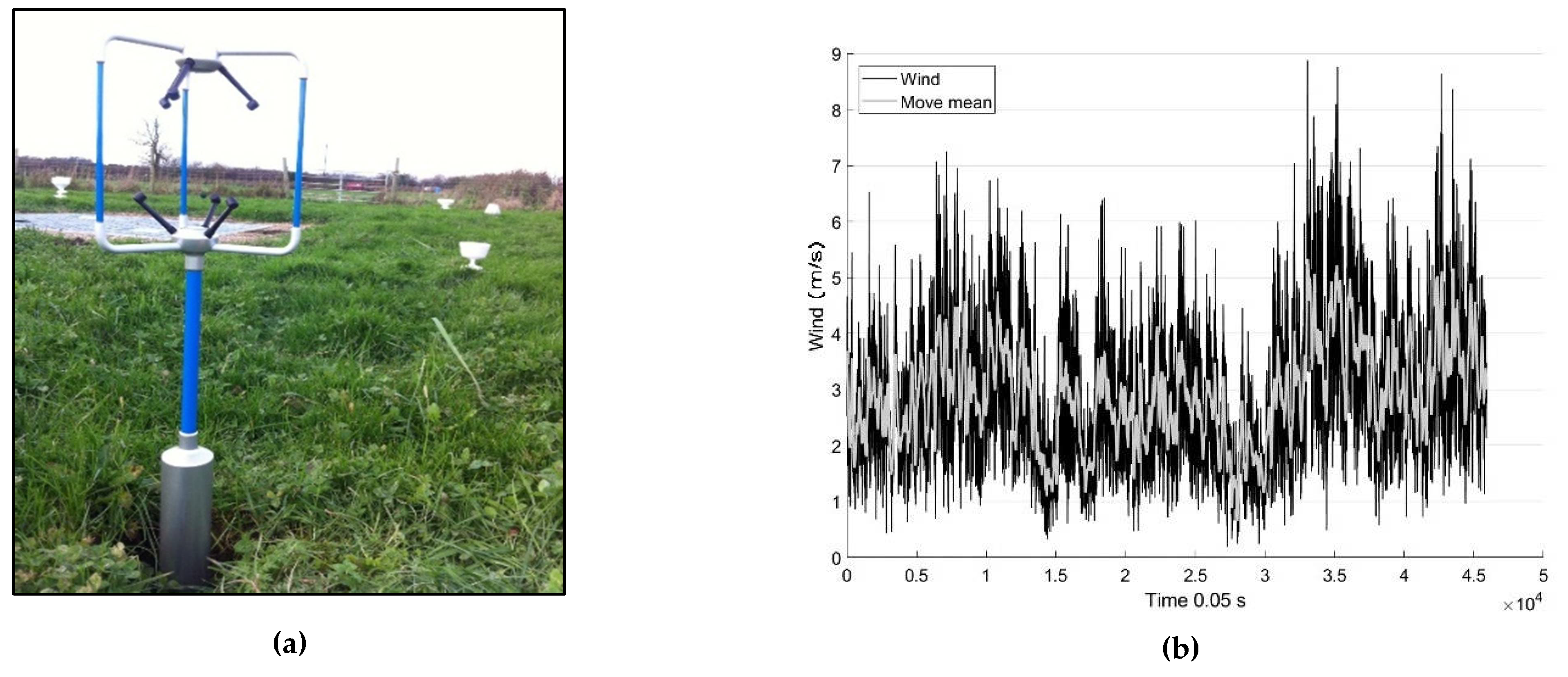
Various studies, mainly focused on the evaluation of the efficiency of wind turbines, report estimates of the free-stream turbulence intensity of natural wind [18,19], generally measured at high elevation (larger than 10 m) above the ground. Precipitation gauges are installed with their collector positioned quite close to the ground surface (usually at about 2 m for gauges supported by poles, and about 0.5 m for gauges directly installed on the ground surface). With the aim of obtaining suitable turbulence intensity values to characterize the wind near the ground surface, 3D sonic anemometer measurements (kindly provided by Environmental Measurements Ltd.—EML©, Newcastle, UK) from the Nafferton (UK) field test site (see Figure 1a) were analyzed. Data were composed of 38 minutes of high-frequency (20 Hz) wind measurements (Figure 1b). The moving average (Figure 1b) was calculated by testing different dimensions of the moving window, N, and checking that the Reynolds average approach was satisfied [20]. This requires that the mean values of the turbulent fluctuations , and in all directions (x, y, z) must be null. A trial-and-error procedure was adopted: after choosing a tentative value for N, the wind measurements were divided in wind classes (defined by their central value Uref from 1 to 5.5 m s−1 with bin size of 0.5 m s−1), based on their average magnitude. For each wind class, the mean of the turbulent fluctuations was calculated, and the N value associated with the minimum of the average fluctuations was chosen (resulting in N = 125). Finally, the relative turbulence intensity values (, and ) for each wind class were calculated as follows:
2.2. CFD Simulations
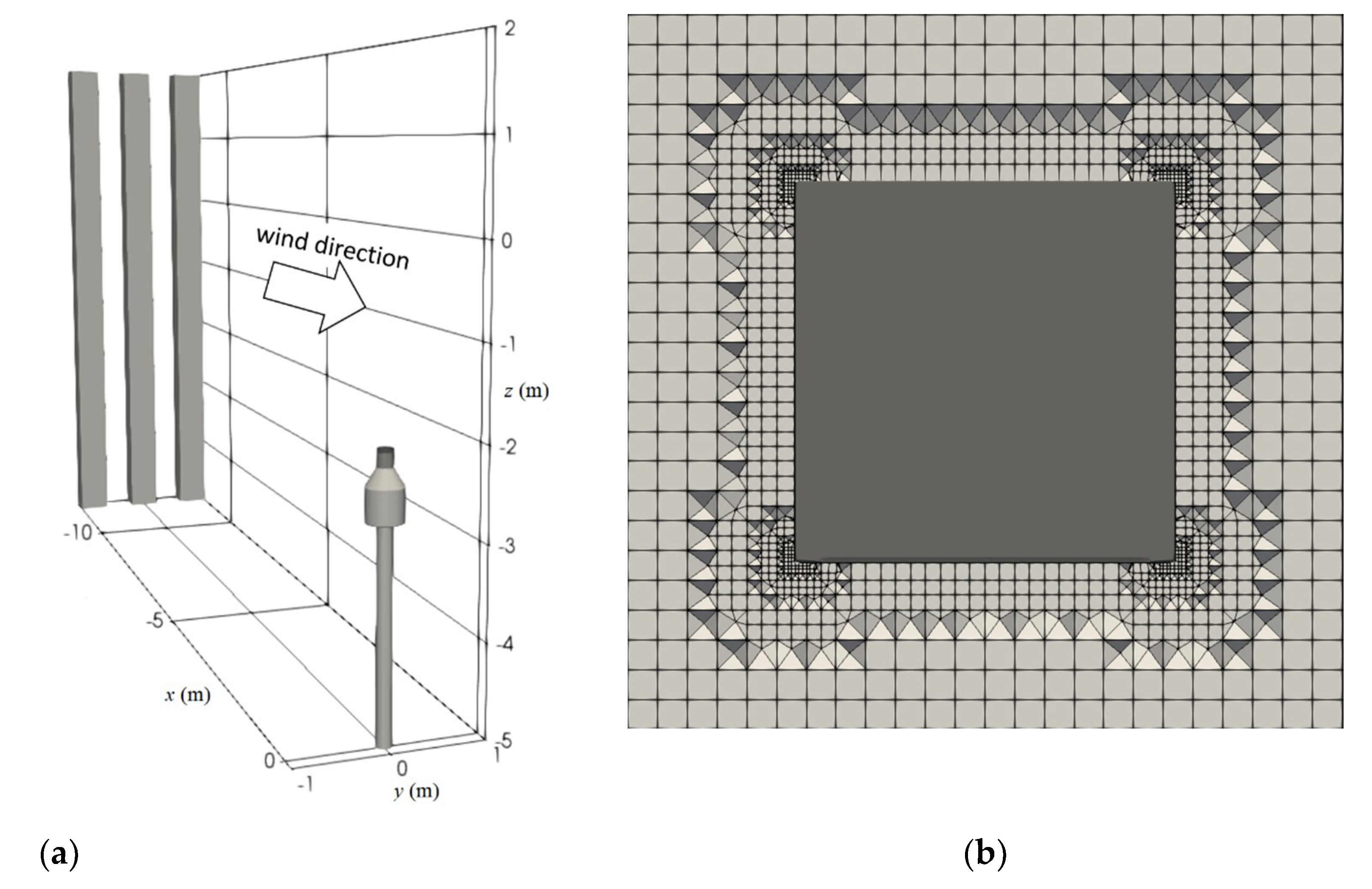
The airflow pattern around a Geonor T200B (hereinafter, Geonor) precipitation gauge was obtained from CFD simulations, under both uniform and turbulent free-stream conditions. The Geonor gauge is a traditional weighing gauge characterized by a “chimney” shape, with an orifice diameter D = 0.160 m and height equal to 0.740 m. To reproduce realistic turbulence conditions near the gauge, three geometrical obstacles (square pillars, 0.3 × 0.3 × 7 m) were introduced in the computational domain upstream of the gauge (Figure 2a).
The model of the gauge geometry and the three pillars used to generate turbulence were prepared in the Standard Triangulation Language (STL) format. The computational domain of dimensions 40 × 20 × 20 m was realized with the x-axis orientated along the stream-wise direction, the y-axis along the crosswise direction, and the z-axis along the vertical direction. The center of the gauge collector was located at (0, 0, −2), and the square pillars were positioned at x = −12 m and spaced by 0.3 m. They extended four meters above and three meters below the elevation of the gauge collector.
The three-dimensional spatial domain was discretized using an unstructured hybrid hexahedral/prismatic finite volume mesh. The computational mesh for the simulation under uniform free-stream conditions was composed of twelve million cells, while by introducing the three pillars, the number of cells reached fourteen million (Figure 2b), with a significant increase in the computational burden. The quality of the mesh was checked by using the geometry parameters of orthogonality, skewness, and aspect ratio [21]. In both cases, the max skewness was lower than 3, the max non-orthogonality was lower than 55, and the maximum aspect ratio was lower than 4.1.
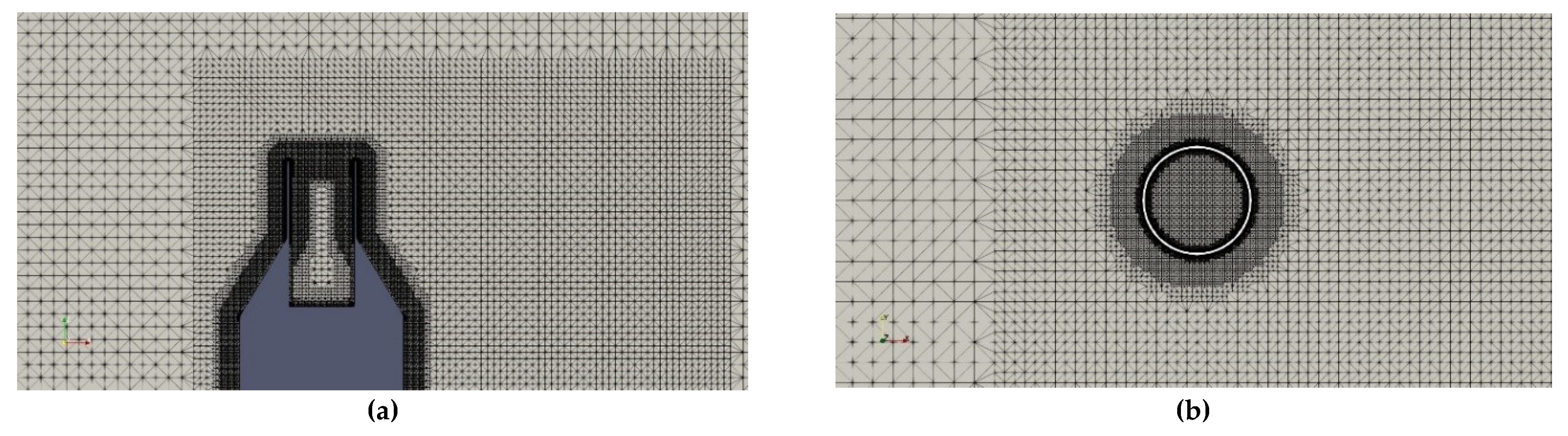
A refinement region (Figure 3a) was realized around the gauge and stretched downwind to improve the numerical solution of the turbulent wake generated by the gauge. Around the gauge body, the computational mesh was discretized with gradually increasing refinements while approaching the gauge surface (Figure 3b). Additional refinement layers were realized close to the surface, and the minimum dimension of the cells nearest to the geometry was about 0.35 mm, corresponding to 1/10 of the collector rim thickness.
To obtain high quality CFD results, we performed LESs. With this numerical approach, the turbulent scales of motion were solved down to the smaller size of the computational mesh. Moreover, under turbulent free-stream conditions, the LES was able to fully reproduce the development of the turbulence wake downstream of the three obstacles before impacting on the gauge body.
The fluid, air, was modelled as a Newtonian incompressible fluid with kinematic viscosity υa = 1.2 × 10⁻⁵ m2 s−1 and density ρa = 1.3 kg m−3 at a reference environmental temperature Ta = 0 °C. For each configuration, at the inlet of the computational domain (y–z plane), the undisturbed wind speed, Uref, was imposed parallel to the x-axis and it was maintained uniform and constant in time, while a null gradient condition was set for pressure. At the outlet y–z plane, opposite to the inlet, a null gradient condition for the velocity and the atmospheric pressure was imposed, while the lateral surfaces of the domain were set as symmetry planes. The ground and the gauge body were assumed as impermeable surfaces with a no-slip condition. In all computational cells, initial conditions were imposed equal to Uref for the velocity and equal to zero for the relative pressure.
The LES approach uses a filtering operation to define a threshold (Equation (2)) between the directly solved turbulent scales and those that are modelled. In Equation (3), is the ith component of velocity, denotes the filtered-scale velocity that is directly solved by the model, and is the subgrid-scale velocity.
Using this notation, the filtering operation can be made general through the convolution integral between and a filter function G:
The Navier–Stokes continuity and momentum equations assume the following form:
The Smagorinsky sub-grid scale approach was adopted to model the sub-grid stresses ) with a gradient-diffusion process in a similar way to a molecular motion, in the form:
where the strain rate tensor () and kinematic eddy viscosity () are:
is the Smagorinsky dimensionless empirical parameter, set equal to 0.2.
2.3. Particle Tracking and Collection Efficiency
Based on the airflow simulation, the improved LPT model proposed in ref [22] was used to model the trajectories of snow particles when approaching the gauge collector. Dry snow particles were chosen because they are the most sensitive to the airflow characteristics, and especially to the acceleration and the vertical and transversal velocity components that are affected by turbulence. The cross-section area, density, and volume of the simulated particles were set in compliance with the power law formulation reported in the work of ref [23]. The modelled particle diameters were set equal to d = 0.25, 0.5, 0.75 mm and from 1 to 8 mm, with bin size of 1 mm. The starting positions of the particles were set on a regular grid located upstream and above the gauge collector. Their terminal velocity was obtained by imposing the equilibrium between the acting forces associated with the gravity acceleration and the aerodynamic drag coefficient. The drag coefficient formulation provided by ref [24] for crystals was employed. For each simulated particle, the initial velocity components were set equal to the undisturbed wind speed in the horizontal direction; the null value along the transversal direction and the terminal velocity, calculated as a function of the particle diameter, in the vertical direction.
For each particle diameter, the number of particles, , which fall inside the gauge collector in disturbed conditions due to the aerodynamic response of the gauge body was calculated from the LPT model. For the two investigated free-stream configurations and for each particle size, we obtained the catch ratio r, defined as the ratio between the number of particles captured by the gauge collector in disturbed airflow conditions, , and the maximum number of particles, captured in undisturbed conditions, .
The integral of the catch ratio on the full range of diameters investigated provides the numerical CE, in the form:
where and are the density and volume of the particles, respectively, is the number of particles which should fall inside the gauge collector if the airflow field was not affected by the aerodynamic response of the gauge body, and is the total number of particles per unit volume of air and per unit size interval having volume equal to the sphere of diameter comprised between d and d + dd.
The method requires the assumption of a suitable PSD, i.e., the distribution of (usually expressed in mm−1 m−3) as a function of the particle diameter d (mm), over the specified range of diameters. In this work, the PSD formulation proposed in ref [25] for dry snow was used, having the characteristic exponential function proposed by ref [26], and obtained by fitting experimental observations:
where mm−1 m−3 is the intercept and Λ mm−1 is the slope of the linear form of the curve in a semi-log plot.
For a widespread mid-latitude rain, a constant value for N0 and a relationship for Λ as a function of the rainfall intensity (RI mm h−1) was found, as follows [26]:
For solid precipitation, based on field experiments, the two parameters of the distribution as a function of the snowfall intensity (SI [mm h−1]) are expressed as follows [25]:
3. Results
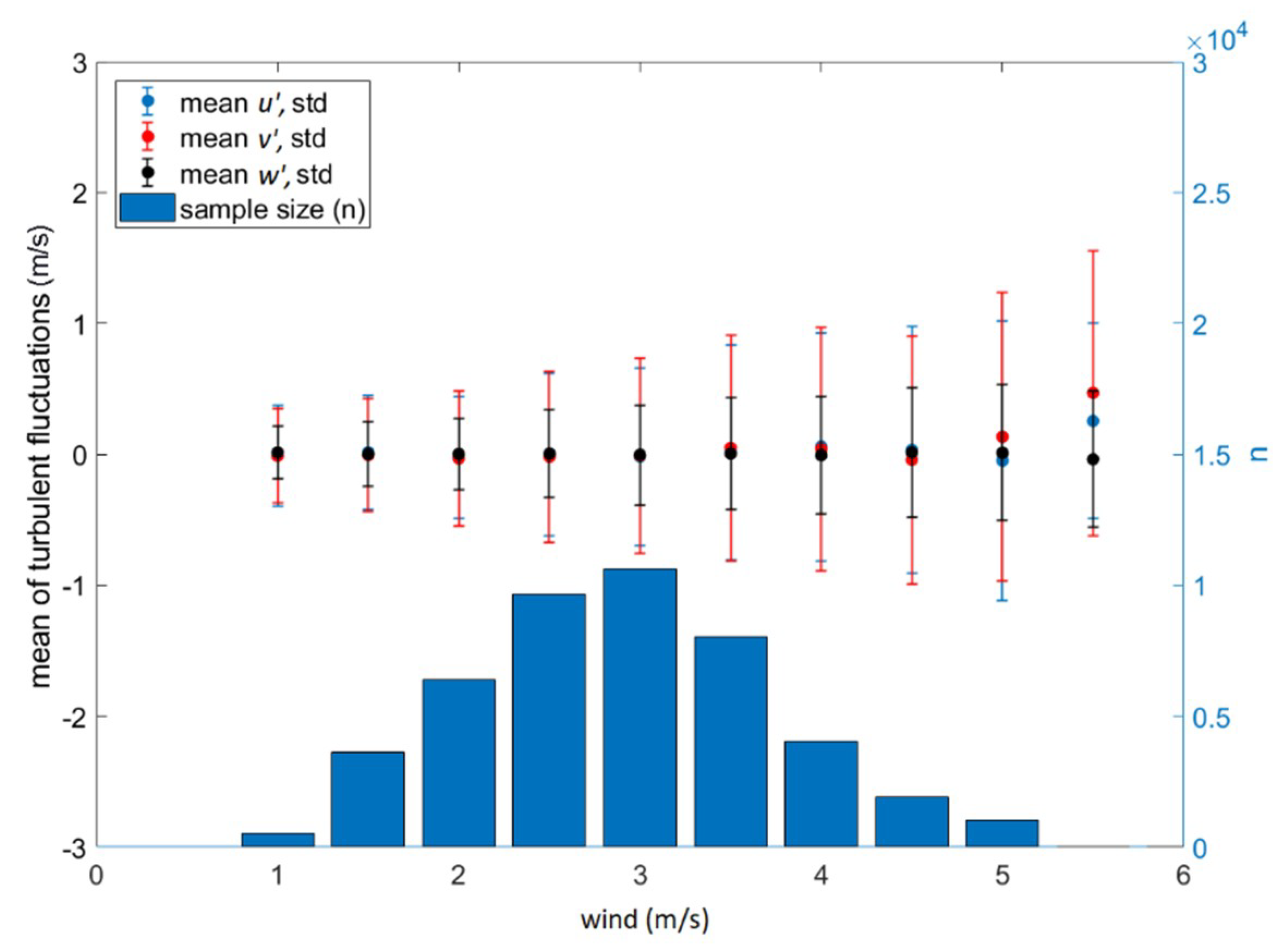
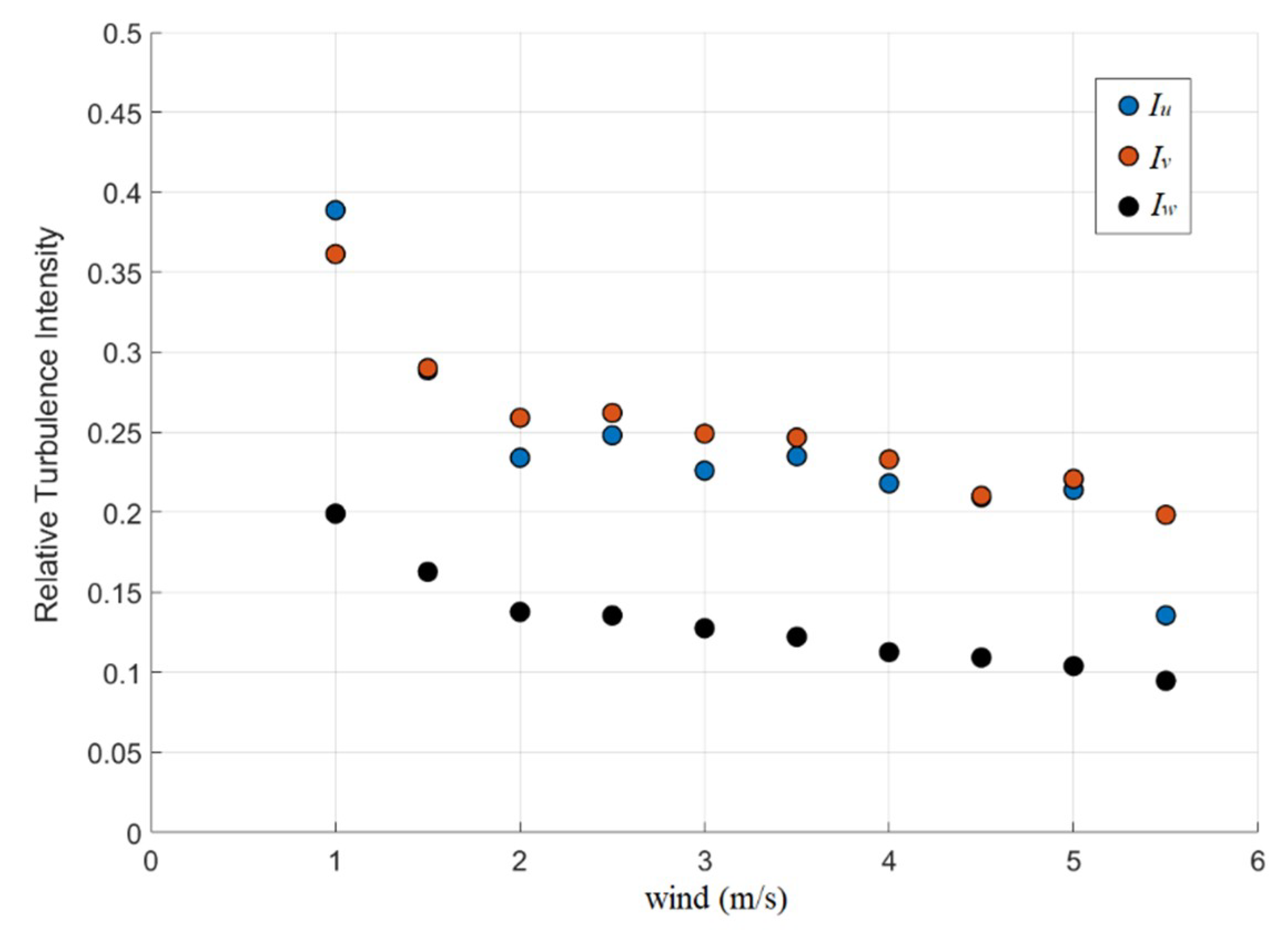
In Figure 4, the mean value of the turbulent fluctuations (circles) and the associated standard deviation (bars) are plotted for each wind class, as derived from the analysis of high-frequency anemometer measurements by setting N = 125. On the right-hand axis, the sample size (histogram) for each wind class is reported. This result reveals that turbulent fluctuations exhibited average values very close to zero, except for the wind classes characterized by a small sample size (wind speed > 5 m s−1). As expected, along the two horizontal directions (x and y) the relative turbulence intensity values (, ) were very similar, while for the vertical direction (z) the relative turbulent intensity values ) were lower (Figure 5). In all cases, the relative turbulence intensity values decreased with increasing wind speed and seemed to have an asymptotical constant limit, although data for high wind speed classes were too few to be conclusive; this behavior is in line with literature observations, albeit referring to higher elevation measurements [19].
To limit the computational burden, for both the investigated free-stream conditions, simulations were performed by imposing a single wind speed, equal to Uref = 6 m s−1, at the inlet surface (upwind y, z plane of the computational domain) as a boundary condition. When the airflow overtook the three obstacles, its mean velocity magnitude decelerated and assumed the value of 2.5 m s−1, which became the new reference wind speed (Uref) for the turbulent free-stream configuration. Thanks to the scalability (low Reynolds dependence) of the mean flow fields under uniform free-stream conditions [11], the CFD results were rescaled by assuming Uref = 2.5 m s−1, to make the results comparable.
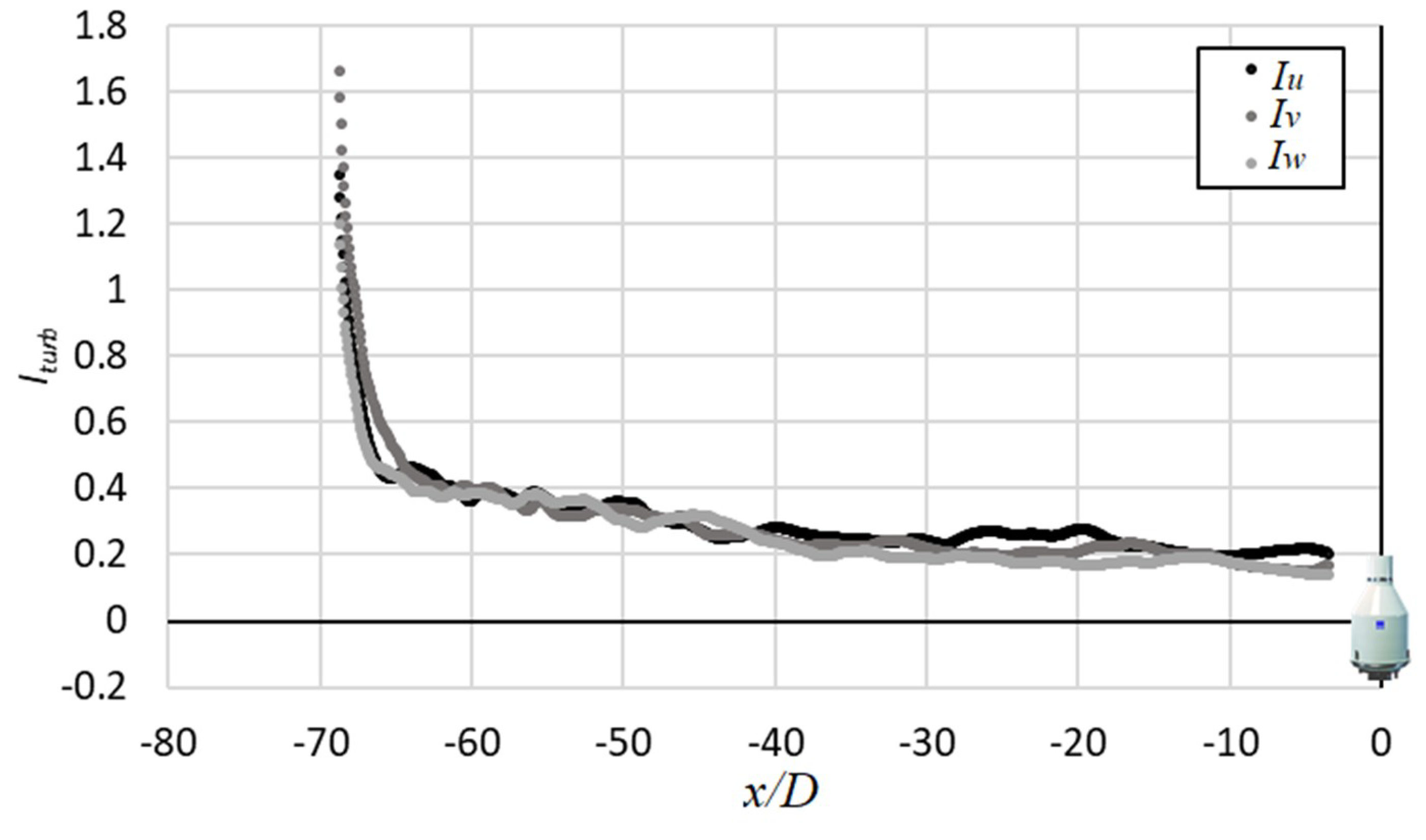
For the free-stream turbulent configuration, the decay along the longitudinal direction (x/D) of the three relative turbulence intensity profiles at the gauge collector elevation and the streamwise symmetry axis is shown in Figure 6. The longitudinal distance (x/D) between the three obstacles and the gauge was calibrated to obtain, at the reference wind speed Uref = 2.5 m s−1, the desired level of turbulence as measured at the Nafferton (U.K.) field test site as = 0.25.
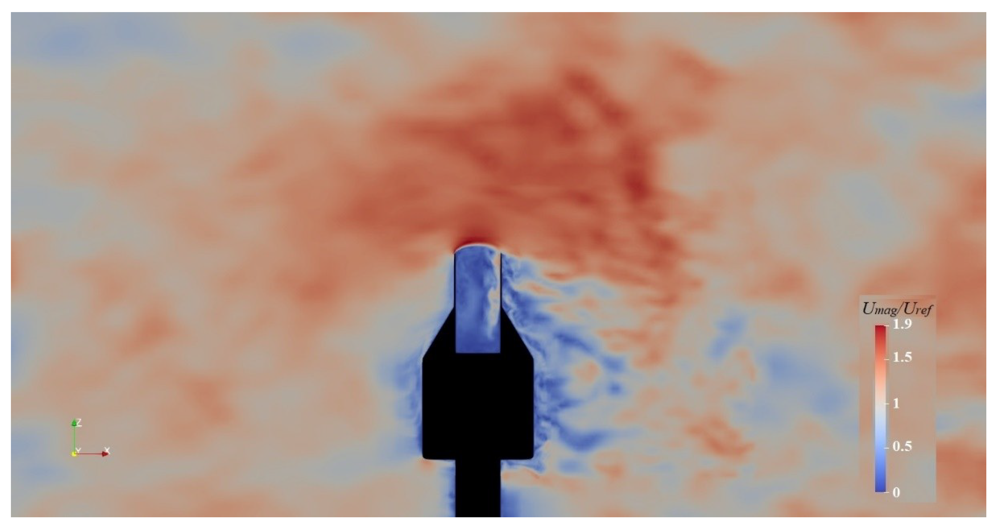
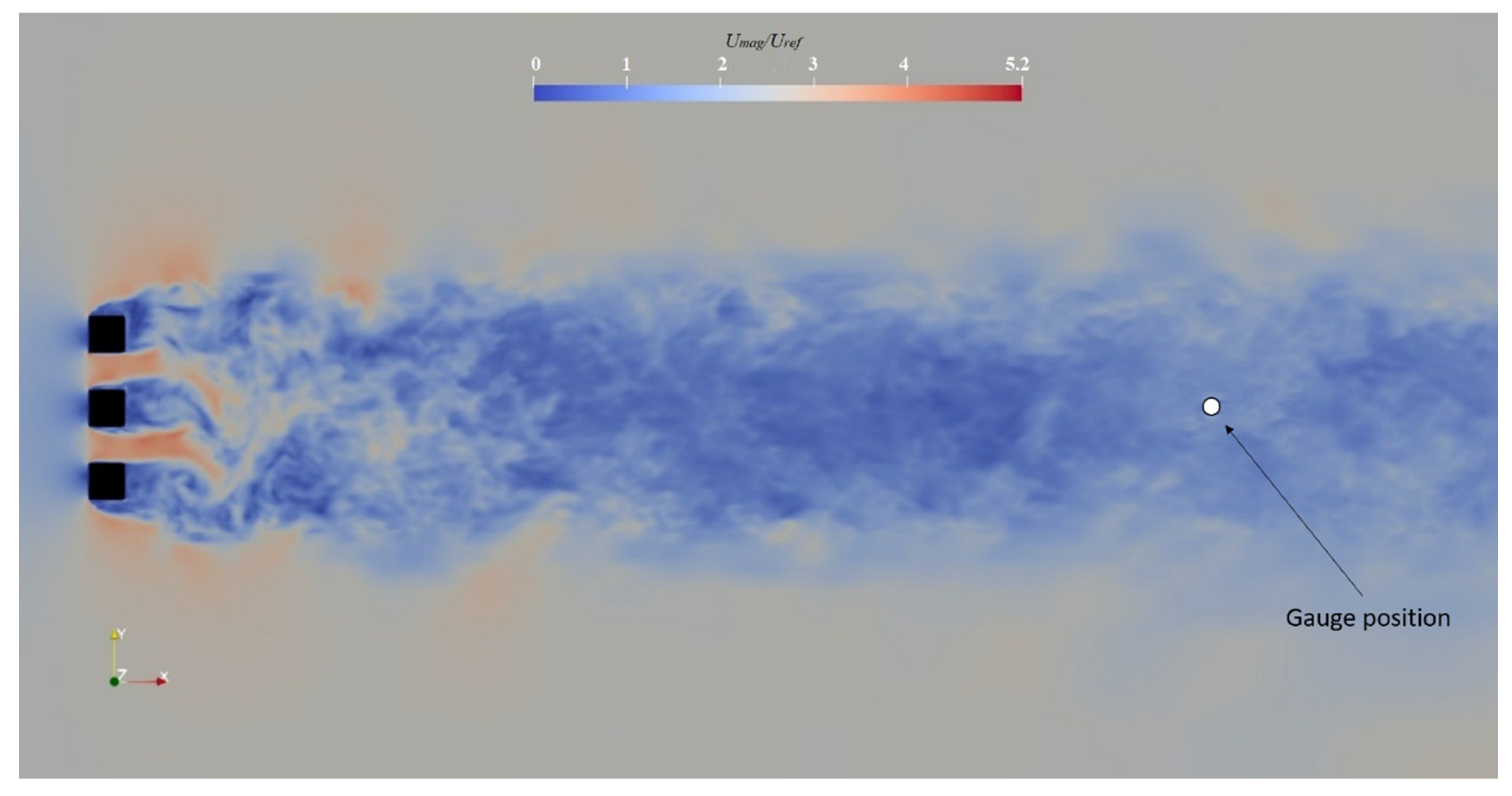
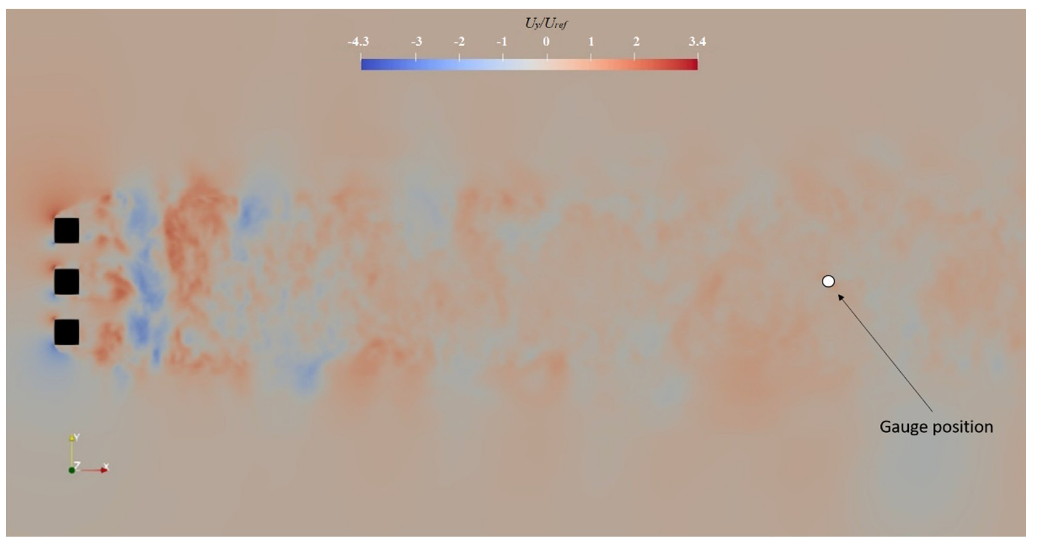
When the free-stream turbulent flow impacts on a gauge body, an accelerated zone (Figure 7) and updraft and downdraft components arise above the collector of the gauge. In this configuration, the gauge collector was totally immersed in the turbulent flow generated by the three obstacles, as shown in Figure 8, where the normalized magnitude (Umag/Uref) of the instantaneous flow velocity in the horizontal plane (x,y) at the gauge collector elevation is reported. Along the transversal direction (y/D), the flow field started to become uniform many diameters away from the collector. As shown in Figure 9, the transversal component of the flow velocity (Uy/Uref) revealed the typical characteristics of vortex shedding which occurred with a regular frequency and with alternate opposite velocity directions.
In addition to the work presented in ref [15], where the free-stream turbulence effect was investigated using an unsteady Reynolds-averaged Navier–Stokes approach (URANS), and results were provided in terms of attenuation of the airflow updraft and acceleration above the collector of the gauge, in the present work the particle–fluid interaction (using a one-way coupled model) was also addressed, and the two free-stream turbulence conditions were compared in terms of catch ratios and collection efficiency.
The LPT model was run upon the mean airflow fields obtained from the LES for each free-stream turbulence condition. The calculated catch ratios for each particle diameter are listed in Table 1. A more pronounced undercatch emerged for small particles (less than 2 mm) under turbulent free-stream conditions with respect to the uniform case, while the opposite occurred for larger particles (d > 2 mm). This was due to the greater aptitude of the small size particles to follow the turbulent velocity fluctuations, while larger particles are more inertial. In particular, the free-stream turbulence had two main effects: it reduced the aerodynamic effect of the wind–gauge interaction, with lower velocity components near the gauge body (as demonstrated in ref [15]) and introduced velocity fluctuations in all directions.
When the particle size is small, particles are more sensitive to the turbulent fluctuations, and therefore catch ratios in uniform free-stream conditions are larger than in turbulent conditions. With increasing the particle size, and therefore its terminal velocity, particle trajectories are less sensitive to the turbulent fluctuations. Moreover, in turbulent free-stream conditions, they cross a less disturbed airflow field so that catch ratios become larger than in uniform free-stream conditions.
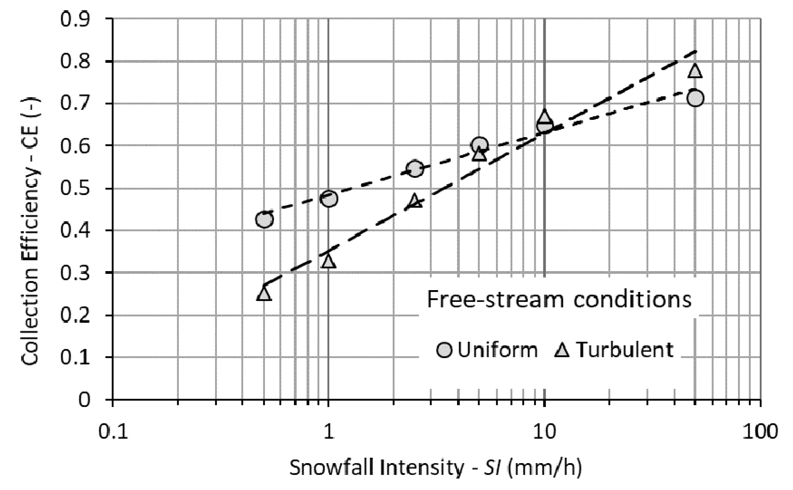
To obtain an overall evaluation of the free-stream turbulence impact on the collection performance of the gauge, the overall CE was computed using Equation 10 with the assumed PSD formulation as proposed in ref [25].
The impact on the CE is indeed modulated by the shape of the PSD. Given the dependence of the PSD on the snowfall intensity, the result is highly dependent on the specific precipitation event. The strong relationship of the CE with the SI was demonstrated by refs 16 and 17 for solid and liquid precipitation, respectively. Following the same approach, the impact of the free-stream turbulence intensity on the CE was calculated here for a set of reference snowfall intensity values from 0.5 to 50 mm h−1.
The CE curves obtained for the uniform and turbulent free-stream conditions at Uref = 2.5 m s−1 are plotted as a function of SI in Figure 10, where an inversion of the sign of the relative difference between the two curves is evident at about 10 mm h−1. Beneath that threshold, neglecting the free-stream turbulence in the simulation would lead to an overestimation of the CE, with a resulting underestimation of the wind-induced error of precipitation measurements. The opposite occurs beyond 10 mm h−1, with an underestimation of the CE that leads to an overestimation of the wind-induced error. Note that the typical snowfall rates are well below that threshold, and the impact of neglecting the free-stream turbulence intensity may lead to an overestimation of the collection efficiency of about 30% at SI = 1 mm h−1 and Uref = 2.5 m s−1.
The inversion in the sign of the relative difference between the CE calculated under uniform and turbulent free-stream conditions can be explained by considering the relative weight of particles smaller than 2 mm (the inversion threshold in the catch ratios reported in Table 1) in the PSD (Figure 11). Indeed, at SI = 1 mm h−1, particles smaller than 2 mm account for about 99.7% of the total number of particles in the unit volume of the atmosphere, which results in about 82.8% of the equivalent water volume. At 10 mm h−1, however, these values become equal to 77% of the total number of particles and 7% of the equivalent water volume.
4. Discussion
The obtained results confirm that neglecting the free-stream turbulence intensity in the numerical simulation of the airflow field leads to a biased assessment of the wind-induced undercatch of catching type precipitation gauges. Further work is needed to quantify this bias for a wide range of wind speed and gauge shape configurations, which does require an extensive numerical effort due to the significant computational burden of the LES approach. This is beyond the scope of the present work, whose aim is to demonstrate the impact of neglecting the free-stream turbulence in the assessment of the collection efficiency, and to explain the underlying physical reasons based on a joint fluid-dynamics and particle–fluid interaction numerical approach. The specific setup chosen to demonstrate this phenomenon made no special assumptions that could limit the validity of the results and their extension to similar configurations of the wind speed, turbulence intensity, PSD, and gauge shape, except for the numerical value of the assumed parameters.
The derived dependence of the impact of turbulence on the snowfall intensity is in agreement with results in the literature and highlights the basic role of the PSD in modulating the collection efficiency, depending on the microphysical characteristics of the specific precipitation event. Additional studies of the link between the mathematical form and parameters of the PSD and precipitation intensity in various meteorological conditions would possibly enhance our understanding of such a modulation effect, leading to more detailed CFD simulations of the exposure problem and quantification of the associated measurement biases. The operational benefit would reside in the derivation of adjustment curves (also called transfer functions in the literature) as a function of both wind velocity and precipitation intensity, which would better reproduce the results of field experiments.
Further consequences are expected on the design and implementation of field experiments, where the traditional setup for the comparison of measurements obtained from test gauges and reference configurations (shielded gauges) should be complemented by including additional measurements obtained from high-resolution three-dimensional anemometers and suitable disdrometers. In this sense, the development of precipitation measurement instruments based on non-catching principles (typically optical) would benefit the contemporary measurement of the PSD and precipitation intensity.
Author Contributions
Conceptualization, A.C., M.C. and L.G.L.; methodology, A.C., M.C. and L.G.L.; software, M.C.; data curation, A.C.; writing—original draft preparation, A.C.; writing—review and editing, M.C. and L.G.L.; supervision, L.G.L. All authors have read and agreed to the published version of the manuscript.
Funding
This research was funded by the Italian MIUR (Ministero dell’Istruzione, dell’Università e della Ricerca), grant number PRIN20154WX5NA, project “Reconciling precipitation with runoff: the role of understated measurement biases in the modelling of hydrological processes”.
Institutional Review Board Statement
Not applicable.
Informed Consent Statement
Not applicable.
Data Availability Statement
Restrictions apply to the availability of these data. Data was obtained from EML© and are available from the authors with the permission of EML©.
Acknowledgments
Data were provided by Environmental Measurements Ltd. (EML©) from the Nafferton (U.K.) field test site and this work was developed as partial fulfilment of the PhD thesis of the first author. Special thanks to the Italian Air Force for providing access to the high-performance computing resources at the ECMWF, within the activities of the CIMO/WMO Lead Centre of Precipitation Intensity through the High-Computing ISCRA class C project “Aerodynamic Response of Precipitation Gauges Immersed in a Turbulent Wind Field”.
Conflicts of Interest
The authors declare no conflict of interest.
References
- Lanza, L.G.; Stagi, L. Certified accuracy of rainfall data as a standard requirement in scientific investigations. Adv. Geosci. 2008, 16, 43–48. [Google Scholar] [CrossRef] [Green Version]
- Sevruk, B. Methods of correction for systematic error in point precipitation measurement for operational use. Adv. WMO. 1982, 21, 106. [Google Scholar]
- Lanza, L.G.; Vuerich, E.; Gnecco, I. Analysis of highly accurate rain intensity measurements from a field test site. Adv. Geosci. 2010, 25, 37–44. [Google Scholar] [CrossRef] [Green Version]
- Jevons, W.S. On the deficiency of rain in an elevated rain-gauge, as caused by wind. Lond. Edinb. Dublin Philos. Mag. J. Sci. 1861, 21, 421–433. [Google Scholar] [CrossRef]
- Warnick, C.C. Experiments with windshields for precipitation gages. Trans. Am. Geophys. Union 1953, 34, 379–388. [Google Scholar] [CrossRef]
- Colli, M. Assessing the accuracy of precipitation gauges: A CFD approach to model wind induced errors. Ph.D. Thesis, University of Genova, Genova, Italy, March 2014. [Google Scholar]
- Alter, J.C. Shielded storage precipitation gages. Mon. Weather. Rev. 1937, 65, 262–265. [Google Scholar] [CrossRef]
- Yang, D.; E Goodison, B.; Metcalfe, J.R.; Louie, P.; Leavesley, G.; Emerson, D.; Hanson, C.L.; Golubev, V.S.; Elomaa, E.; Gunther, T.; et al. Quantification of precipitation measurement discontinuity induced by wind shields on national gauges. Water Resour. Res. 1999, 35, 491–508. [Google Scholar] [CrossRef]
- Kochendorfer, J.; Rasmussen, R.; Wolff, M.; Baker, B.; Hall, M.E.; Meyers, T.; Landolt, S.; Jachcik, A.; Isaksen, K.; Brækkan, R.; et al. The quantification and correction of wind-induced precipitation measurement errors. Hydrol. Earth Syst. Sci. 2017, 21, 1973–1989. [Google Scholar] [CrossRef] [Green Version]
- Wolff, M.A.; Isaksen, K.; Petersenoverleir, A.; Ødemark, K.; Reitan, T.; Brækkan, R. Derivation of a new continuous adjustment function for correcting wind-induced loss of solid precipitation: Results of a Norwegian field study. Hydrol. Earth Syst. Sci. 2015, 19, 951–967. [Google Scholar] [CrossRef]
- Colli, M.; Lanza, L.G.; Rasmussen, R.; Thériault, J.M. The Collection Efficiency of Shielded and Unshielded Precipitation Gauges. Part I: CFD Airflow Modeling. J. Hydrometeorol. 2015, 17, 231–243. [Google Scholar] [CrossRef] [Green Version]
- Colli, M.; Pollock, M.D.; Stagnaro, M.; Lanza, L.G.; Dutton, M.; O’Connell, E. A Computational Fluid-Dynamics Assessment of the Improved Performance of Aerodynamic Rain Gauges. Water Resour. Res. 2018, 54, 779–796. [Google Scholar] [CrossRef]
- Nešpor, V.; Sevruk, B. Estimation of Wind-Induced Error of Rainfall Gauge Measurements Using a Numerical Simulation. J. Atmospheric Ocean. Technol. 1999, 16, 450–464. [Google Scholar] [CrossRef]
- Cauteruccio, A.; Chinchella, E.; Stagnaro, M.; Lanza, L.G. Snow Particle Collection Efficiency and Adjustment Curves for the Hotplate© Precipitation Gauge. J. Hydrometeorol. 2021. [Google Scholar] [CrossRef]
- Cauteruccio, A.; Colli, M.; Freda, A.; Stagnaro, M.; Lanza, L.G. The Role of Free-Stream Turbulence in Attenuating the Wind Updraft above the Collector of Precipitation Gauges. J. Atmospheric Ocean. Technol. 2020, 37, 103–113. [Google Scholar] [CrossRef]
- Colli, M.; Stagnaro, M.; Lanza, L.G.; Rasmussen, R.; Thériault, J.M. Adjustments for Wind-Induced Undercatch in Snowfall Measurements Based on Precipitation Intensity. J. Hydrometeorol. 2020, 21, 1039–1050. [Google Scholar] [CrossRef] [Green Version]
- Cauteruccio, A.; Lanza, L.G. Parameterization of the Collection Efficiency of a Cylindrical Catching-Type Rain Gauge Based on Rainfall Intensity. Water 2020, 12, 3431. [Google Scholar] [CrossRef]
- Kumer, V.-M.; Reuder, J.; Dorninger, M.; Zauner, R.; Grubišić, V. Turbulent kinetic energy estimates from profiling wind LiDAR measurements and their potential for wind energy applications. Renew. Energy 2016, 99, 898–910. [Google Scholar] [CrossRef] [Green Version]
- Øistad, I.S. Analysis of the Turbulence Intensity at Skipheia Measurement Station. Master’s Thesis, Norwegian University of Science and Technology, Trondheim, Norway, June 2015. [Google Scholar]
- Cauteruccio, A. The role of turbulence in particle-fluid interaction as induced by the outer geometry of catching-type precipitation gauges. Ph.D. Thesis, University of Genova, Genova, Italy, April 2020. [Google Scholar]
- Jasak, H.; Jemcov, A.; Tukovic, Z. OpenFOAM: A C++ Library for Complex Physics Simulations. In Proceedings of the International Workshop on Coupled Methods in Numerical Dynamics IUC, Dubrovnik, Croatia, 19–21 September 2007; Available online: http://cmnd2007.fsb.hr/proc/jasak.pdf (accessed on 30 January 2021).
- Colli, M.; Rasmussen, R.; Thériault, J.M.; Lanza, L.G.; Baker, C.B.; Kochendorfer, J. An Improved Trajectory Model to Evaluate the Collection Performance of Snow Gauges. J. Appl. Meteorol. Clim. 2015, 54, 1826–1836. [Google Scholar] [CrossRef] [Green Version]
- Thériault, J.M.; Rasmussen, R.; Ikeda, K.; Landolt, S. Dependence of Snow Gauge Collection Efficiency on Snowflake Characteristics. J. Appl. Meteorol. Clim. 2012, 51, 745–762. [Google Scholar] [CrossRef] [Green Version]
- Khvorostyanov, V.I.; A Curry, J. Fall Velocities of Hydrometeors in the Atmosphere: Refinements to a Continuous Analytical Power Law. J. Atmospheric Sci. 2005, 62, 4343–4357. [Google Scholar] [CrossRef]
- Gunn, K.L.S.; Marshall, J.S. The Distribution with Size of Aggregate Snowflakes. J. Meteorol. 1958, 15, 452–461. [Google Scholar] [CrossRef] [Green Version]
- Marshall, J.S.; Palmer, W.M.K. The distribution of raindrops with size. J. Meteor. 1948, 5, 165–166. [Google Scholar] [CrossRef]
Figure 1.
(a) The Nafferton (U.K.) field test site with the 3D Sonic anemometer and EML© aerodynamic rain gauges installed at the ground surface, and (b) high-frequency wind measurements (black line) and moving average with N = 125 (grey line).
Figure 1.
(a) The Nafferton (U.K.) field test site with the 3D Sonic anemometer and EML© aerodynamic rain gauges installed at the ground surface, and (b) high-frequency wind measurements (black line) and moving average with N = 125 (grey line).

Figure 2.
(a) Portion of the geometric setup with the three pillars positioned upstream of the gauge, and the wind direction indicated by the white arrow. (b) Horizontal section (x,y plane) and gradual refinement of the computational mesh close to one sample pillar at a generic elevation.
Figure 2.
(a) Portion of the geometric setup with the three pillars positioned upstream of the gauge, and the wind direction indicated by the white arrow. (b) Horizontal section (x,y plane) and gradual refinement of the computational mesh close to one sample pillar at a generic elevation.

Figure 3.
(a) Refinement region around the Geonor gauge body in the central vertical section (x,z plane at y = 0) and (b) gradual refinement close to its surface in the horizontal section at the gauge collector elevation (x,y plane at z = −2 m).
Figure 3.
(a) Refinement region around the Geonor gauge body in the central vertical section (x,z plane at y = 0) and (b) gradual refinement close to its surface in the horizontal section at the gauge collector elevation (x,y plane at z = −2 m).

Figure 4.
Mean values and standard deviations of turbulent fluctuations (left-hand axis) and sample size (right-hand axis) for each wind class, measured by a 3D sonic anemometer at the Nafferton (U.K.) field test site.
Figure 4.
Mean values and standard deviations of turbulent fluctuations (left-hand axis) and sample size (right-hand axis) for each wind class, measured by a 3D sonic anemometer at the Nafferton (U.K.) field test site.

Figure 5.
Relative turbulence intensity for the three Cartesian directions for each wind class, measured by a 3D sonic anemometer at the Nafferton (U.K.) field test site.
Figure 5.
Relative turbulence intensity for the three Cartesian directions for each wind class, measured by a 3D sonic anemometer at the Nafferton (U.K.) field test site.

Figure 6.
Decrease of the three numerical relative turbulence intensity profiles at the gauge collector elevation along the spatial domain between the position of the obstacles (x/D = −70) and the gauge (x/D = 0).
Figure 6.
Decrease of the three numerical relative turbulence intensity profiles at the gauge collector elevation along the spatial domain between the position of the obstacles (x/D = −70) and the gauge (x/D = 0).

Figure 7.
Normalized magnitude (Umag/Uref) of the instantaneous flow velocity in the vertical plane (x,z) at y/D = 0 for the turbulent free-stream conditions.
Figure 7.
Normalized magnitude (Umag/Uref) of the instantaneous flow velocity in the vertical plane (x,z) at y/D = 0 for the turbulent free-stream conditions.

Figure 8.
Normalized magnitude of the instantaneous flow velocity (Umag/Uref) in the horizontal plane (x,y) at the gauge collector elevation for the turbulent free-stream conditions.
Figure 8.
Normalized magnitude of the instantaneous flow velocity (Umag/Uref) in the horizontal plane (x,y) at the gauge collector elevation for the turbulent free-stream conditions.

Figure 9.
Normalized transversal component (Uy/Uref) of the instantaneous flow velocity in the horizontal plane (x,y) at the gauge collector elevation for the turbulent free-stream conditions.
Figure 9.
Normalized transversal component (Uy/Uref) of the instantaneous flow velocity in the horizontal plane (x,y) at the gauge collector elevation for the turbulent free-stream conditions.

Figure 10.
CE curves as a function of SI, obtained under uniform and turbulent free-stream conditions at Uref = 2.5 m s−1.
Figure 10.
CE curves as a function of SI, obtained under uniform and turbulent free-stream conditions at Uref = 2.5 m s−1.

Figure 11.
Percentage number and volume of particles having a diameter less than 2 mm within a unit volume of the atmosphere, based on the assumed particle size distribution (PSD).
Figure 11.
Percentage number and volume of particles having a diameter less than 2 mm within a unit volume of the atmosphere, based on the assumed particle size distribution (PSD).


Table 1.
Catch ratios obtained for each solid particle size d at Uref = 2.5 m s−1 using the LPT model and based on the large eddy simulation (LES) mean airflow fields for the Geonor precipitation gauge under uniform and turbulent free-stream conditions.
Table 1.
Catch ratios obtained for each solid particle size d at Uref = 2.5 m s−1 using the LPT model and based on the large eddy simulation (LES) mean airflow fields for the Geonor precipitation gauge under uniform and turbulent free-stream conditions.
| d (mm) | 0.25 | 0.5 | 0.75 | 1 | 2 | 3 | 4 | 5 | 6 | 7 | 8 |
|---|---|---|---|---|---|---|---|---|---|---|---|
| Uniform | 0.190 | 0.393 | 0.449 | 0.492 | 0.590 | 0.659 | 0.708 | 0.734 | 0.757 | 0.787 | 0.787 |
| Turbulent | 0.164 | 0.164 | 0.216 | 0.289 | 0.590 | 0.718 | 0.777 | 0.820 | 0.849 | 0.869 | 0.892 |
Publisher’s Note: MDPI stays neutral with regard to jurisdictional claims in published maps and institutional affiliations. |
© 2021 by the authors. Licensee MDPI, Basel, Switzerland. This article is an open access article distributed under the terms and conditions of the Creative Commons Attribution (CC BY) license (http://creativecommons.org/licenses/by/4.0/).
Share and Cite
MDPI and ACS Style
Cauteruccio, A.; Colli, M.; Lanza, L.G. On Neglecting Free-Stream Turbulence in Numerical Simulation of the Wind-Induced Bias of Snow Gauges. Water 2021, 13, 363. https://doi.org/10.3390/w13030363
AMA Style
Cauteruccio A, Colli M, Lanza LG. On Neglecting Free-Stream Turbulence in Numerical Simulation of the Wind-Induced Bias of Snow Gauges. Water. 2021; 13(3):363. https://doi.org/10.3390/w13030363
Chicago/Turabian StyleCauteruccio, Arianna, Matteo Colli, and Luca G. Lanza. 2021. "On Neglecting Free-Stream Turbulence in Numerical Simulation of the Wind-Induced Bias of Snow Gauges" Water 13, no. 3: 363. https://doi.org/10.3390/w13030363
Note that from the first issue of 2016, this journal uses article numbers instead of page numbers. See further details here.