
Potential Dam Breach Analysis and Flood Wave Risk Assessment Using HEC-RAS and Remote Sensing Data: A Multicriteria Approach

 ,
, 

 , and
, and
Abstract
:1. Introduction
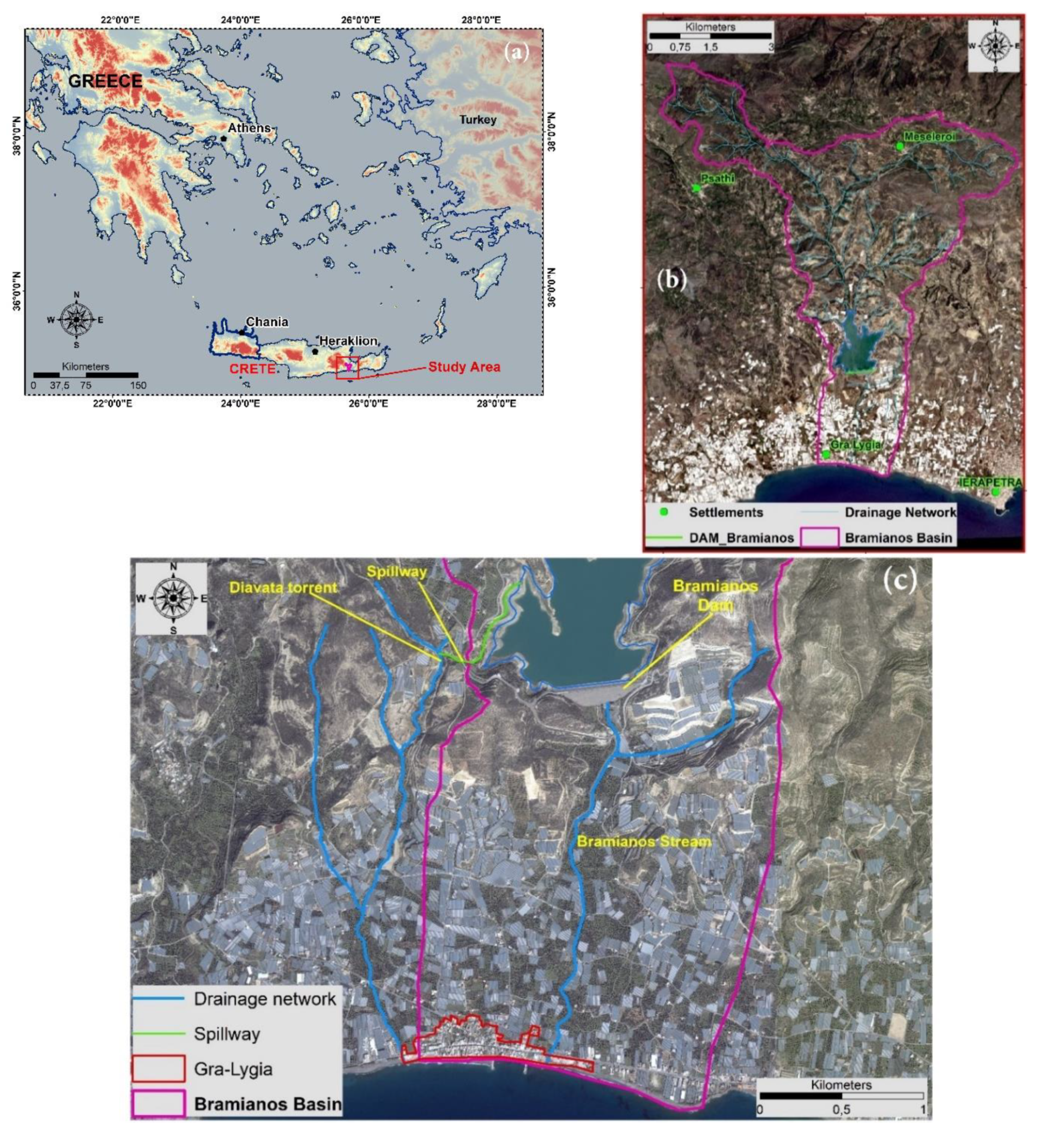
2. Study Area
2.1. Watershed Characteristics
2.2. Dam Characteristics
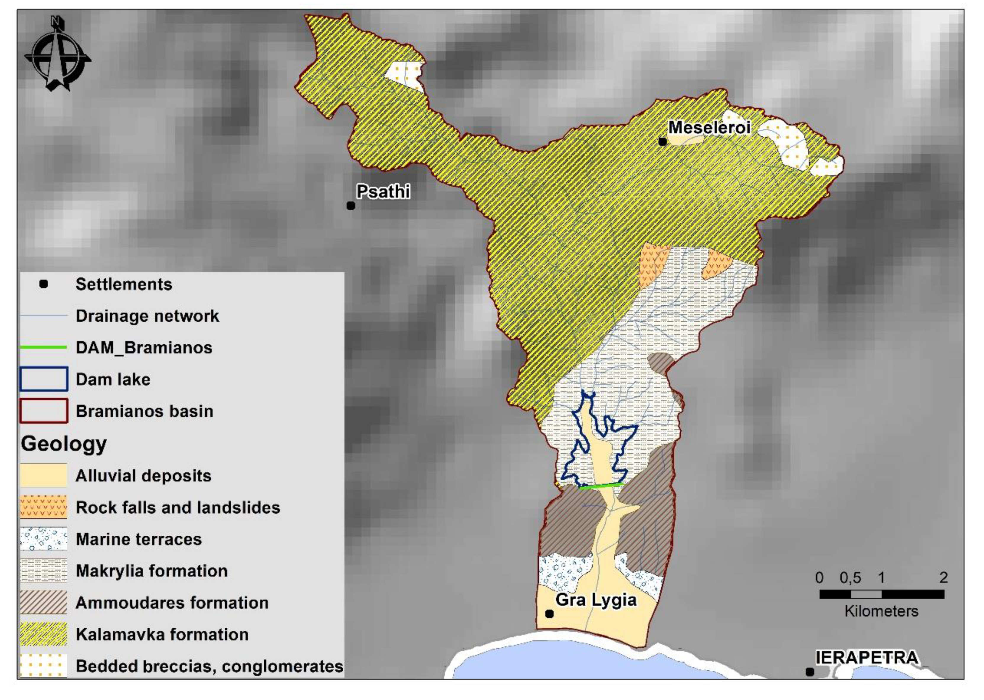
2.3. Geological and Hydrolithological Characteristics
3. Dam Breach Mechanisms and Flood Wave Impact Overview
4. Materials and Methods
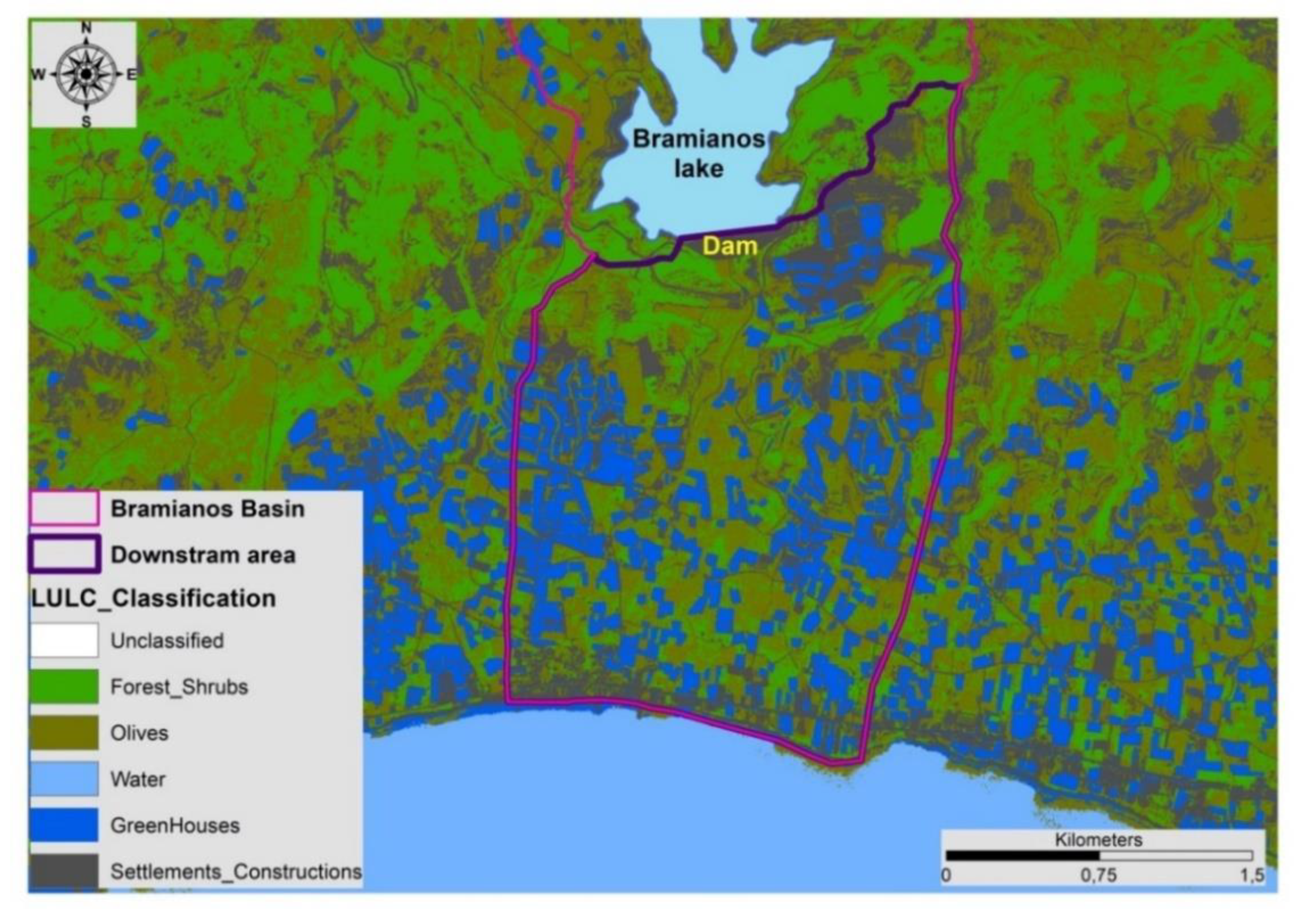
4.1. Orthophotos and Sentinel-2 Data—LULC Mapping
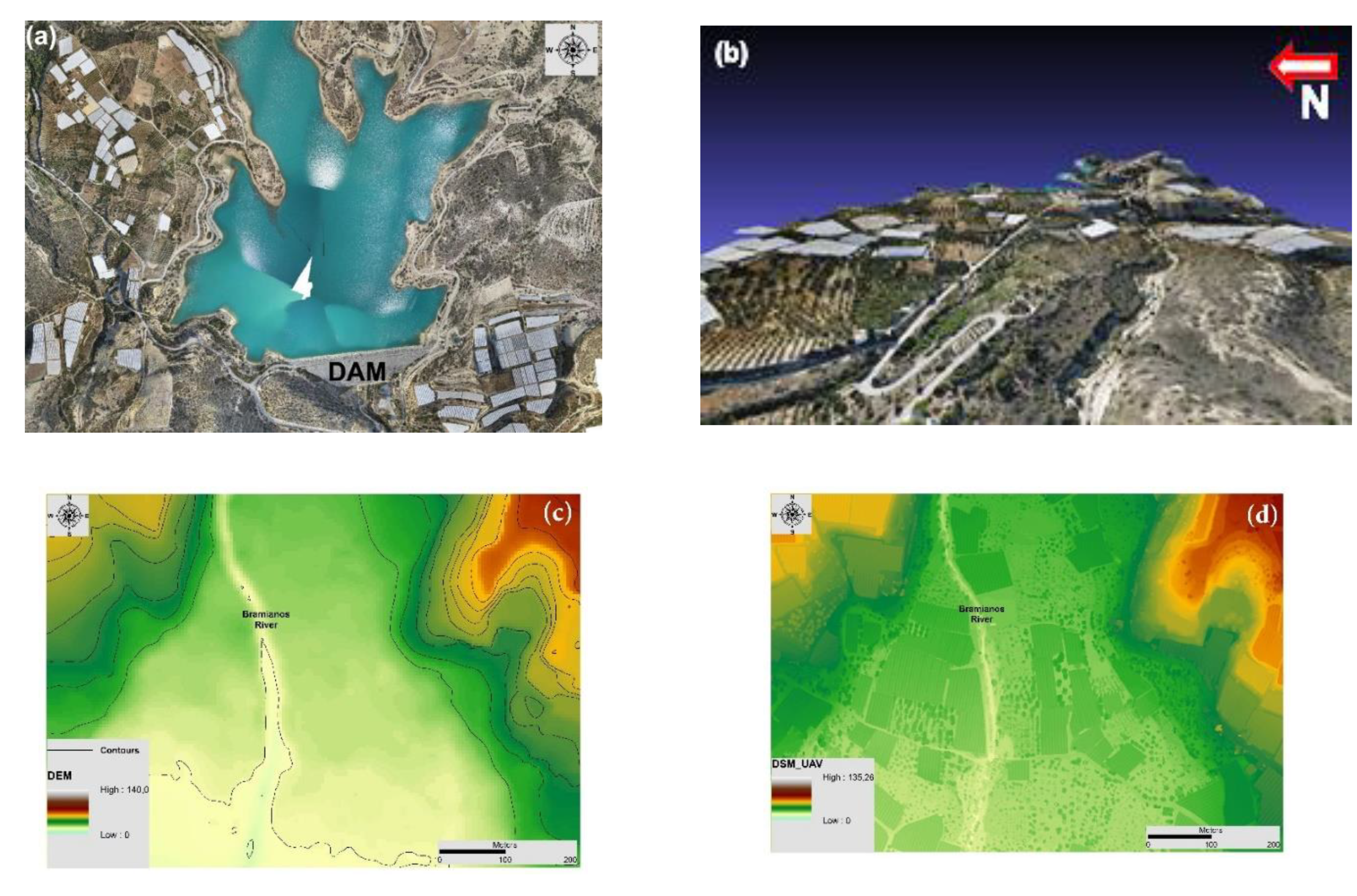
4.2. Unmanned Aerial System (UAS)—Digital Surface Model
4.3. Digital Elevation Model
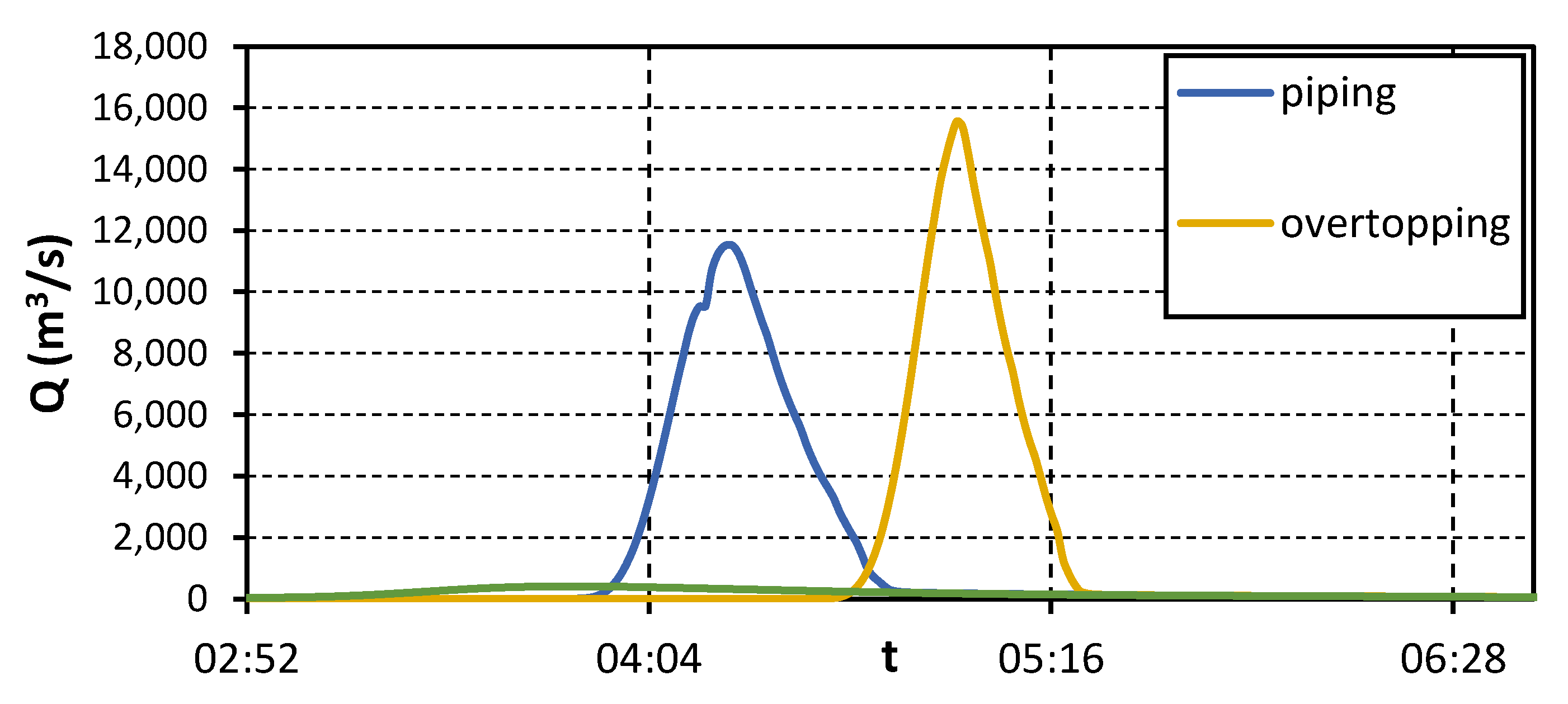
4.4. Simulation Models of Dam Failure Mechanisms
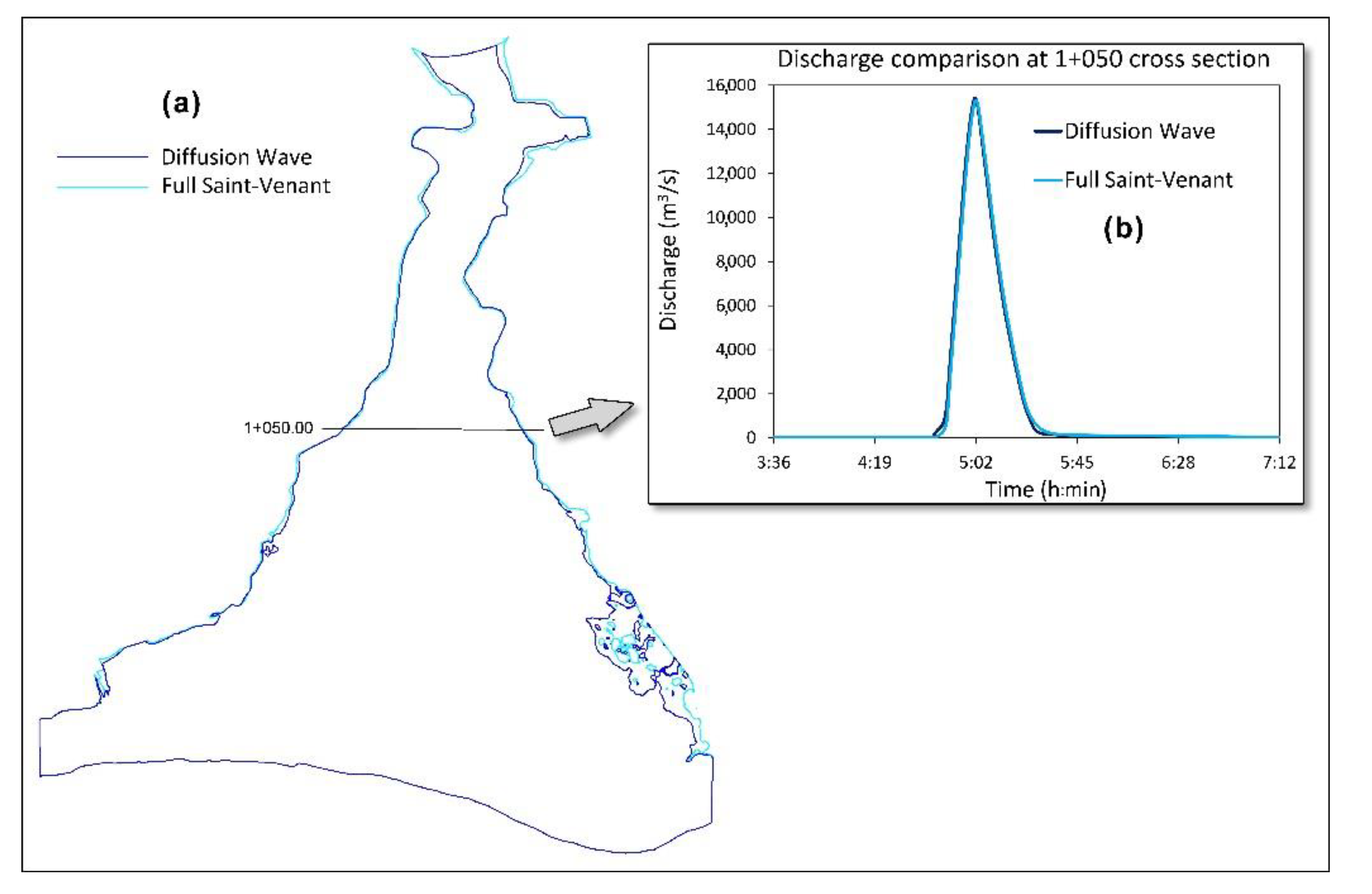
4.5. Hydraulic Model Analysis
4.6. Flood Hazard Assessment
5. Results
5.1. LULC Results and Validation
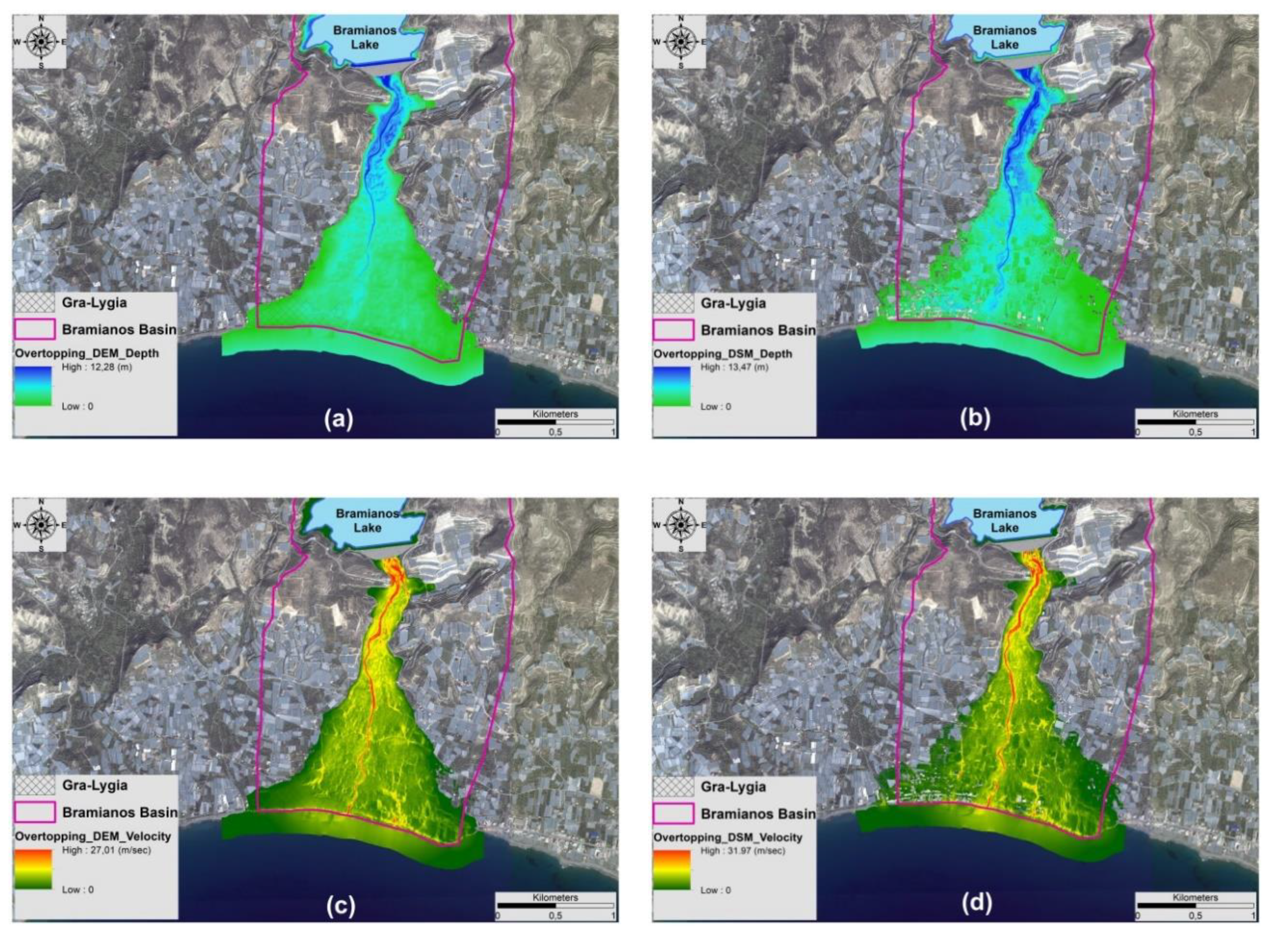
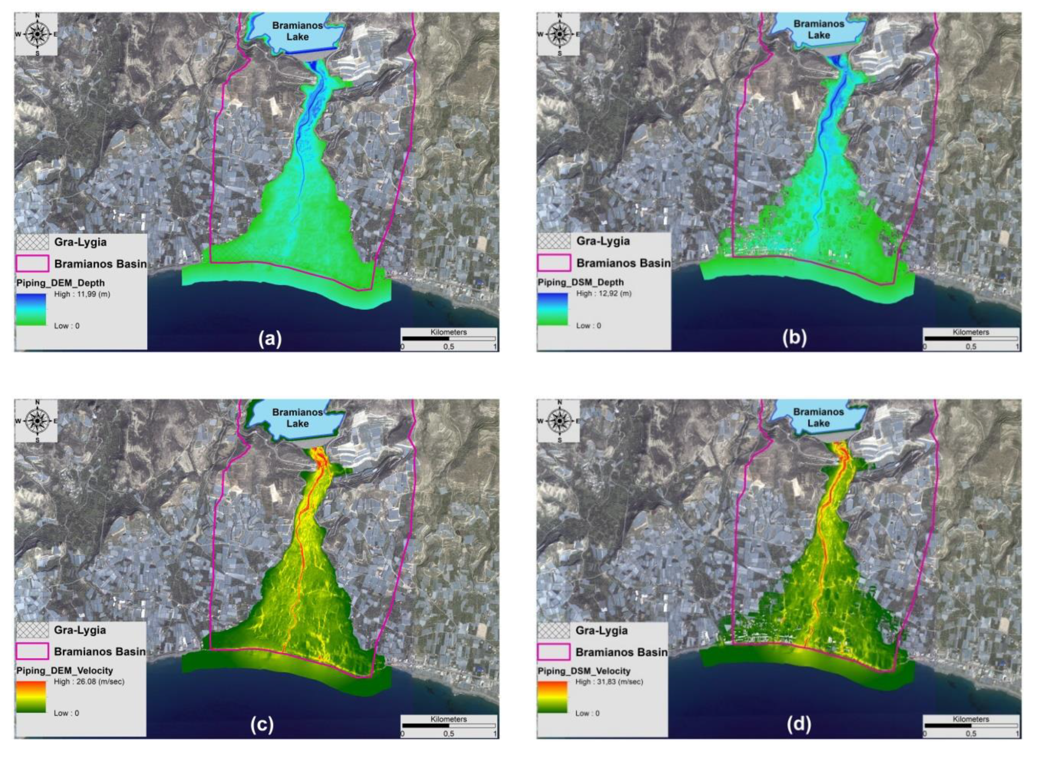
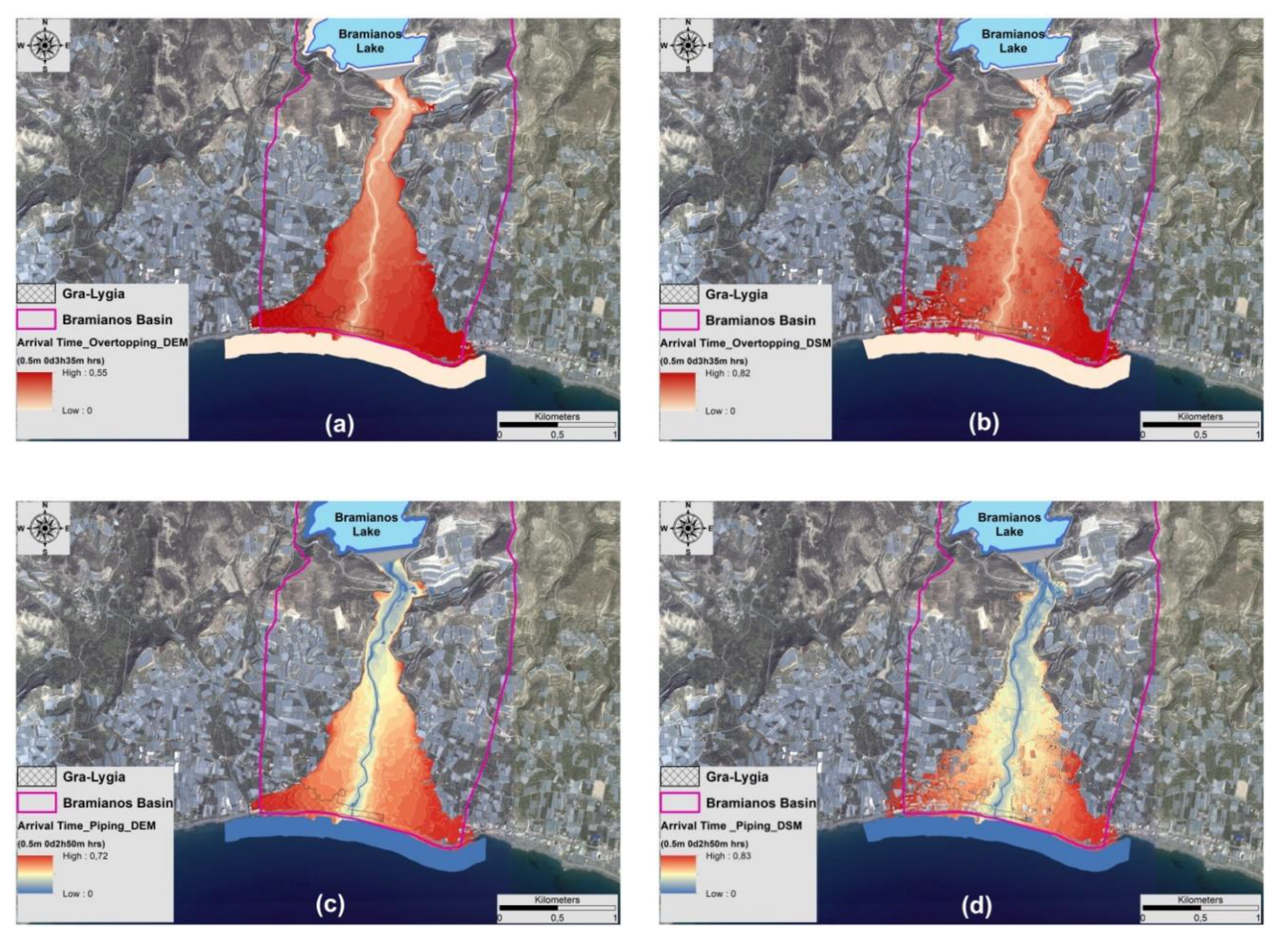
5.2. Floodextents, Depths, Velocities and Arrival Time Estimation for the Two Elevation Profiles and the Two Dam Failure Mechanisms
5.3. Flooded Areas
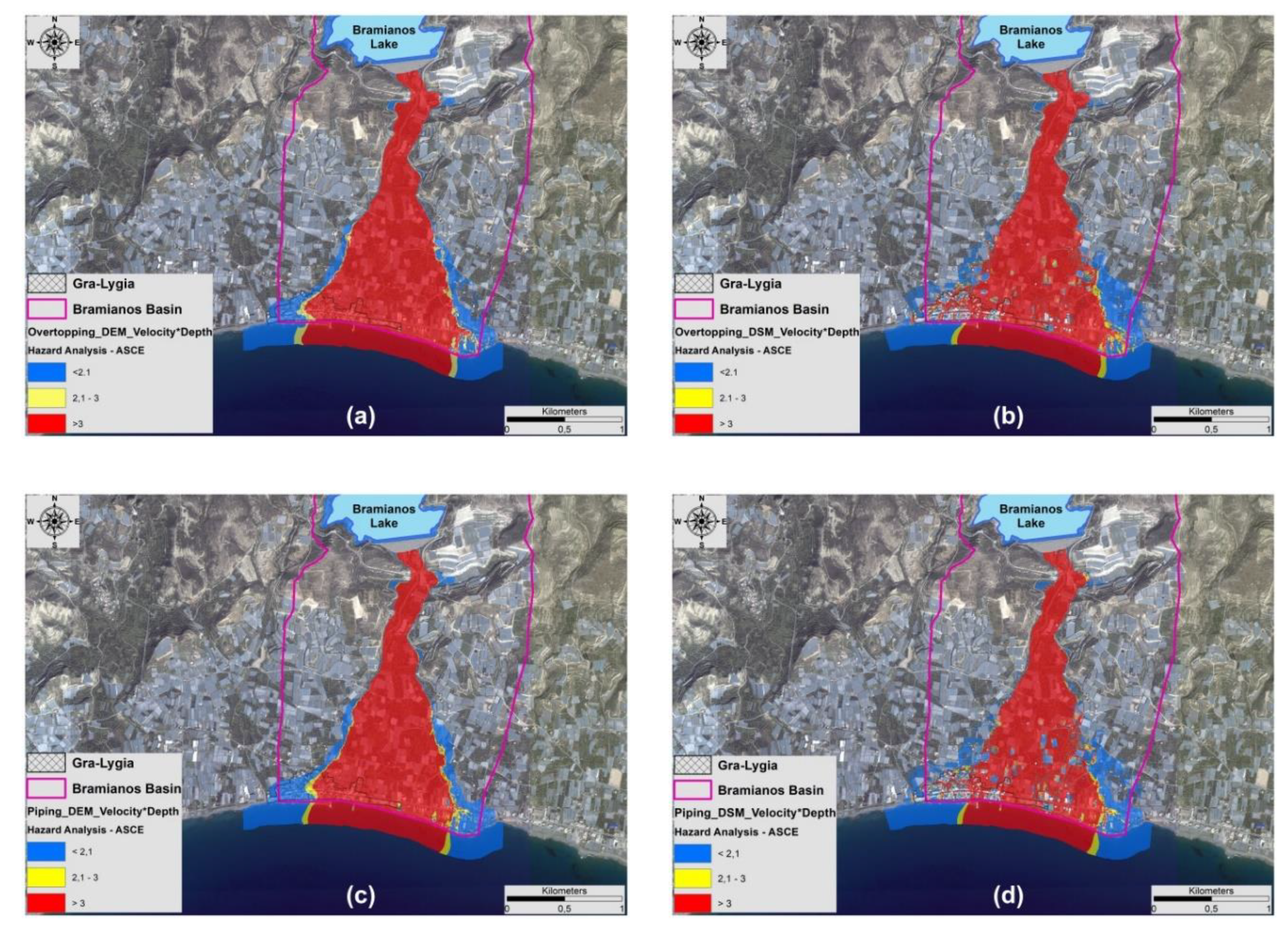
5.4. Hazard Relation to Depth and Velocity Results
6. Discussion
7. Conclusions
Author Contributions
Funding
Institutional Review Board Statement
Informed Consent Statement
Data Availability Statement
Acknowledgments
Conflicts of Interest
References
- Mirauda, D.; Albano, R.; Sole, A.; Adamowski, J. Smoothed particle hydrodynamics modeling with advanced boundary conditions for two-dimensional dam-break floods. Water 2020, 12, 1142. [Google Scholar] [CrossRef] [Green Version]
- Ge, W.; Jiao, Y.; Sun, H.; Li, Z.; Zhang, H.; Zheng, Y.; Guo, X.; Zhang, Z.; van Gelder, P.H.A.J.M. A Method for Fast Evaluation of Potential Consequences of Dam Breach. Water 2019, 11, 2224. [Google Scholar] [CrossRef] [Green Version]
- Li, W.; Li, Z.; Ge, W.; Wu, S. Risk Evaluation Model of Life Loss Caused by Dam-break Flood and Its Application. Water 2019, 11, 1359. [Google Scholar] [CrossRef] [Green Version]
- Mao, J.; Wang, S.; Ni, J.; Xi, C.; Wang, J. Management System for Dam-Break Hazard Mapping in a Complex Basin Environment. ISPRS Int. J. Geo-Inf. 2017, 6, 162. [Google Scholar] [CrossRef] [Green Version]
- Xiong, Y. A Dam Break Analysis Using HEC-RAS. J. Water Resour. Prot. 2011. [Google Scholar] [CrossRef]
- Penman, A.D.M. Monkswood Reservoir-the leaking Bath water. In Proceedings of the 11th British Dam Society Conference, London, UK, 14–17 June 2000; pp. 377–387. [Google Scholar]
- Types of Dams. British Dam Society. Available online: http://www.britishdams.org (accessed on 2 May 2020).
- Costa, J.E.; Schuster, R.L. The formation and failure of natural dams. GSA Bull. 1988, 100, 1054–1068. [Google Scholar] [CrossRef]
- Pytharouli, S.I. Study of the Long-Term Behaviour of Kremasta Dam Based on the Analysis of Geodetic Data and Reservoir Level Fluctuations; University of Patras: Patras, Greece, 2007. [Google Scholar]
- Ge, W.; Li, Z.; Liang, R.Y.; Li, W.; Cai, Y. Methodology for Establishing Risk Criteria for Dams in Developing Countries, Case Study of China. Water Resour. Manag. 2017, 31, 4063–4074. [Google Scholar] [CrossRef]
- Luino, F.; Tosatti, G.; Bonaria, V. Bonaria Dam Failures in the 20th Century: Nearly 1000 Avoidable Victims in Italy Alone. J. Environ. Sci. Eng. 2014, 3, 19–31. [Google Scholar]
- Brown, C.A.; Graham, W.J. Assessing the threat to life from Dam failure. J. Am. Water Resour. Assoc. 1988, 24, 1303–1309. [Google Scholar] [CrossRef]
- Pistrika, A.; Tsakiris, G. Hypothetical dam break: Loss of life estimation in flood risk assessment. In Proceedings of the 1st Panhellenic Conference of large dams; Technical Chamber of Greece: Larissa, Greek, 2008; p. 13. [Google Scholar]
- Albu, L.-M.; Enea, A.; Iosub, M.; Breabăn, I.-G. Dam Breach Size Comparison for Flood Simulations. A HEC-RAS Based, GIS Approach for Drăcșani Lake, Sitna River, Romania. Water 2020, 12, 1090. [Google Scholar] [CrossRef]
- International Commission on large dams (ICOLD). Lessons from Dam Incidents; ICOLD: Paris, France, 1978. [Google Scholar]
- Viseu, T.; de Almeida, A.B. Dam-break risk management and hazard mitigation. State Art Sci. Eng. 2009, 36, 211–239. [Google Scholar]
- Wu, M.; Ge, W.; Li, Z.; Wu, Z.; Zhang, H.; Li, J.; Pan, Y. Improved Set Pair Analysis and Its Application to Environmental Impact Evaluation of Dam Break. Water 2019, 11, 821. [Google Scholar] [CrossRef] [Green Version]
- Zhong, Q.M.; Chen, S.S.; Deng, Z.; Mei, S.A. Prediction of Overtopping-Induced Breach Process of Cohesive Dams. J. Geotech. Geoenviron. Eng. 2019, 145, 04019012. [Google Scholar] [CrossRef]
- Foster, M.; Fell, R.; Spannagle, M. The statistics of embankment dam failures and accidents. Can. Geotech. J. 2000, 37, 1000–1024. [Google Scholar] [CrossRef]
- Psomiadis, E.; Soulis, K.X.; Zoka, M.; Dercas, N. Synergistic approach of remote sensing and gis techniques for flash-flood monitoring and damage assessment in Thessaly plain area, Greece. Water 2019, 11, 448. [Google Scholar] [CrossRef] [Green Version]
- Qi, H.; Altinakar, M.S. A GIS-based decision support system for integrated flood management under uncertainty with two dimensional numerical simulations. Environ. Model. Softw. 2011, 26, 817–821. [Google Scholar] [CrossRef]
- Hartmann, T.; Spit, T. Implementing the European flood risk management plan. J. Environ. Plan. Manag. 2016, 59, 360–377. [Google Scholar] [CrossRef]
- Eleutério, J. Flood Risk Analysis: Impact of Uncertainty in Hazard Modelling and Vulnerability Assessments on Damage Estimations. Ph.D. Thesis, University of Strasbourg, Strasbourg, France, 2012. [Google Scholar]
- Dasallas, L.; Kim, Y.; An, H. Case Study of HEC-RAS 1D–2D Coupling Simulation: 2002 Baeksan Flood Event in Korea. Water 2019, 11, 2048. [Google Scholar] [CrossRef] [Green Version]
- Butt, M.J.; Umar, M.; Qamar, R. Dam Break Flood Routing Using HEC-RAS and NWS-FLDWAV | Impacts of Global Climate Change. Nat. Hazards 2013, 65, 241–242. [Google Scholar] [CrossRef]
- Teng, J.; Jakeman, A.J.; Vaze, J.; Croke, B.F.W.; Dutta, D.; Kim, S. Flood inundation modelling: A review of methods, recent advances and uncertainty analysis. Environ. Model. Softw. 2017, 90, 201–216. [Google Scholar] [CrossRef]
- Anees, M.T.; Abdullah, K.; Nordin, M.N.M.; Rahman, N.N.N.A.; Syakir, M.I.; Kadir, M.O.A. One- and Two-Dimensional Hydrological Modelling and Their Uncertainties. In Flood Risk Management; InTech: London, UK, 2017. [Google Scholar]
- Casas, A.; Benito, G.; Thorndycraft, V.R.; Rico, M. The topographic data source of digital terrain models as a key element in the accuracy of hydraulic flood modelling. Earth Surf. Process. Landf. 2006, 31, 444–456. [Google Scholar] [CrossRef]
- Merwade, V.; Cook, A.; Coonrod, J. GIS techniques for creating river terrain models for hydrodynamic modeling and flood inundation mapping. Environ. Model. Softw. 2008, 23, 1300–1311. [Google Scholar] [CrossRef]
- Chormanski, J.; Okruszko, T.; Ignar, S.; Batelaan, O.; Rebel, K.T.; Wassen, M.J. Flood mapping with remote sensing and hydrochemistry: A new method to distinguish the origin of flood water during floods. Ecol. Eng. 2011, 37, 1334–1349. [Google Scholar] [CrossRef]
- Sarhadi, A.; Soltani, S.; Modarres, R. Probabilistic flood inundation mapping of ungauged rivers: Linking GIS techniques and frequency analysis. J. Hydrol. 2012, 458–459, 68–86. [Google Scholar] [CrossRef]
- Kavvadias, A.; Psomiadis, E.; Chanioti, M.; Tsitouras, A.; Toulios, L.; Dercas, N. Unmanned Aerial Vehicle (UAV) data analysis for fertilization dose assessment. In Proceedings of the SPIE-The International Society for Optical Engineering, Warsaw, Poland, 2 November 2017; Volume 10421. [Google Scholar]
- Jung, C.-G.; Kim, S.-J. Comparison of the Damaged Area Caused by an Agricultural Dam-Break Flood Wave Using HEC-RAS and UAV Surveying. Agric. Sci. 2017, 08, 1089–1104. [Google Scholar] [CrossRef] [Green Version]
- Mourato, S.; Fernandez, P.; Pereira, L.; Moreira, M. Improving a DSM Obtained by Unmanned Aerial Vehicles for Flood Modelling. IOP Conf. Ser. Earth Environ. Sci. 2017, 95, 022014. [Google Scholar] [CrossRef]
- Kavvadias, A.; Psomiadis, E.; Chanioti, M.; Gala, E.; Michas, S. Precision agriculture-Comparison and evaluation of innovative very high resolution (UAV) and LandSat data. In Proceedings of the 17th International Conference on Information and Communication Technologies in Agriculture Food and Environment-HAICTA, Kavala, Greece, 17–20 September 2015; Volume 1498. [Google Scholar]
- Leventi, I.; Nalbantis, I.; Georgopoulos, A. On the use of Digital Surface Models and hydrological/hydraulic models for inundated area delineation. In Environmental Hydraulics; Stamou, E.H.-C., Ed.; Taylor & Francis Group: London, UK, 2010; pp. 875–880. ISBN 978-0-415-58475-3. [Google Scholar]
- Uysal, M.; Toprak, A.S.; Polat, N. DEM generation with UAV Photogrammetry and accuracy analysis in Sahitler hill. Meas. J. Int. Meas. Confed. 2015, 73, 539–543. [Google Scholar] [CrossRef]
- Oczipka, M.; Bemmann, J.; Piezonka, H.; Munkabayar, J.; Ahrens, B.; Achtelik, M.; Lehmann, F. Small drones for geo-archaeology in the steppe: Locating and documenting the archaeological heritage of the Orkhon Valley in Mongolia. In Proceedings of the Remote Sensing for Environmental Monitoring, GIS Applications, and Geology IX; Michel, U., Civco, D.L., Eds.; SPIE: Bellingham, WA, USA, 2009; p. 747806. [Google Scholar]
- Chang, A.; Jung, J.; Maeda, M.M.; Landivar, J. Crop height monitoring with digital imagery from Unmanned Aerial System (UAS). Comput. Electron. Agric. 2017, 141, 232–237. [Google Scholar] [CrossRef]
- Liu, B.; Shi, Y.; Duan, Y.; Wu, W. UAV-based crops classification with joint features from orthoimage and DSM data. ISPRS Int. Arch. Photogramm. Remote Sens. Spat. Inf. Sci. 2018, XLII-3, 1023–1028. [Google Scholar] [CrossRef] [Green Version]
- Saksena, S.; Merwade, V. Incorporating the effect of DEM resolution and accuracy for improved flood inundation mapping. J. Hydrol. 2015, 530, 180–194. [Google Scholar] [CrossRef] [Green Version]
- Psomiadis, E. Flash flood area mapping utilising Sentinel-1 radar data. In Proceedings of the SPIE-The International Society for Optical Engineering, Edinburgh, UK, 18 October 2016; Volume 10005. [Google Scholar]
- Efthimiou, N.; Psomiadis, E.; Panagos, P. Fire severity and soil erosion susceptibility mapping using multi-temporal Earth Observation data: The case of Mati fatal wildfire in Eastern Attica, Greece. Catena 2020, 187. [Google Scholar] [CrossRef] [PubMed]
- Chatziantoniou, A.; Petropoulos, G.P.; Psomiadis, E. Co-Orbital Sentinel 1 and 2 for LULC mapping with emphasis on wetlands in a mediterranean setting based on machine learning. Remote Sens. 2017, 9, 1259. [Google Scholar] [CrossRef] [Green Version]
- Efthimiou, N.; Psomiadis, E. The Significance of Land Cover Delineation on Soil Erosion Assessment. Environ. Manag. 2018, 62, 383–402. [Google Scholar] [CrossRef] [PubMed]
- Psomiadis, E.; Soulis, K.X.; Efthimiou, N. Using SCS-CN and earth observation for the comparative assessment of the hydrological effect of gradual and abrupt spatiotemporal land cover changes. Water 2020, 12, 1386. [Google Scholar] [CrossRef]
- Soulis, K.X.; Valiantzas, J.D. Identification of the SCS-CN Parameter Spatial Distribution Using Rainfall-Runoff Data in Heterogeneous Watersheds. Water Resour. Manag. 2013, 27, 1737–1749. [Google Scholar] [CrossRef]
- Nourani, V.; Fard, A.F.; Niazi, F.; Gupta, H.V.; Goodrich, D.C.; Kamran, K.V. Implication of remotely sensed data to incorporate land cover effect into a linear reservoir-based rainfall-runoff model. J. Hydrol. 2015, 529, 94–105. [Google Scholar] [CrossRef]
- Sun, Z.; Li, X.; Fu, W.; Li, Y.; Tang, D. Long-term effects of land use/land cover change on surface runoff in urban areas of Beijing, China. J. Appl. Remote Sens. 2013, 8, 084596. [Google Scholar] [CrossRef] [Green Version]
- Mihu-Pintilie, A.; Cîmpianu, C.I.; Stoleriu, C.C.; Pérez, M.N.; Paveluc, L.E. Using High-Density LiDAR Data and 2D Streamflow Hydraulic Modeling to Improve Urban Flood Hazard Maps: A HEC-RAS Multi-Scenario Approach. Water 2019, 11, 1832. [Google Scholar] [CrossRef] [Green Version]
- Albano, R.; Mancusi, L.; Adamowski, J.; Cantisani, A.; Sole, A. A GIS Tool for Mapping Dam-Break Flood Hazards in Italy. ISPRS Int. J. Geo-Inf. 2019, 8, 250. [Google Scholar] [CrossRef] [Green Version]
- Ridolfi, E.; Buffi, G.; Venturi, S.; Manciola, P. Accuracy Analysis of a Dam Model from Drone Surveys. Sensors 2017, 17, 1777. [Google Scholar] [CrossRef] [Green Version]
- Gaki-Papanastassiou, K.; Karymbalis, E.; Papanastassiou, D.; Maroukian, H. Quaternary marine terraces as indicators of neotectonic activity of the Ierapetra normal fault SE Crete (Greece). Geomorphology 2009, 104, 38–46. [Google Scholar] [CrossRef]
- Fortuin, A.R.; Peters, J.M. The Prina Complex in eastern Crete and its relationship to possible Miocene strike-slip tectonics. J. Struct. Geol. 1984, 6, 459–476. [Google Scholar] [CrossRef]
- Sarris, A.; Karakoudis, S.; Vidaki, C.; Soupios, P. Study of the Morphological Attributes of Crete through the Use of Remote Sensing Techniques. IASME Trans. 2005, 6, 1043–1051. [Google Scholar]
- Authority, H.S. Demographic characteristics 2011. Available online: https://www.statistics.gr/el/statistics/-/publication/SAM03/2011 (accessed on 3 July 2020).
- Ministry of Environment and Energy Floods. Available online: https://ypen.gov.gr/perivallon/ydatikoi-poroi/plimmyres/ (accessed on 24 January 2021).
- Dimas, P.; Daniil, E.I.; Michas, S.; Lazaridou, S.L.; Tomanis, L. Finding optimal policies for reservoir system management through stochastic simulation: The case of Bramianos-Myrtos irrigation system in Ierapetra, Crete (In Greek). In Proceedings of the 3rd Panhellenic Conference on Dams and Reservoirs: Project Management and Development Perspectives, Athens, Greece, 12–15 October 2017; p. 14. [Google Scholar]
- Moutopoulos, D.K.; Mantzavrakos, E.S.; Ramfos, A.; Katselis, G. Human-made system, Human-induced Ichthyofauna (Bramianos reservoir, Crete). In Proceedings of the HydroMedit 2018, 3rd International Congress on Applied Ichtyology & Aquatic Enviroment, Volos, Greece, 8–11 November 2018; pp. 726–727. [Google Scholar]
- Pavlakis, P.P.; Dermitzakis, M.D.; Drinia, M.; Antonarakou, A.; Tsourou, T. Paleobiogeographical reconstruction of the Katharo plain. Biol. Gall. 1999, 25, 157–186. [Google Scholar]
- Pichon, X.L.; Angelier, J. The hellenic arc and trench system: A key to the neotectonic evolution of the eastern mediterranean area. Tectonophysics 1979, 60, 1–42. [Google Scholar] [CrossRef]
- Psomiadis, E.; Papazachariou, A.; Soulis, K.X.; Alexiou, D.S.; Charalampopoulos, I. Landslide mapping and susceptibility assessment using geospatial analysis and earth observation data. Land 2020, 9, 133. [Google Scholar] [CrossRef]
- Angelier, J. Determination of the mean principal directions of stresses for a given fault population. Tectonophysics 1979, 56, T17–T26. [Google Scholar] [CrossRef]
- Armijo, R.; Lyon-Caen, H.; Papanastassiou, D. East-west extension and Holocene normal-fault scarps in the Hellenic arc. Geology 1992, 20, 491–494. [Google Scholar] [CrossRef]
- Veliz, V. Fault displacement rates and recent activity on the Ierapetra Fault Zone, Crete, Greece. AGUFM 2015, 2015, T31A-2851. [Google Scholar]
- Caputo, R.; Catalano, S.; Monaco, C.; Romagnoli, G.; Tortorici, G.; Tortorici, L. Active faulting on the island of Crete (Greece). Geophys. J. Int. 2010, 183, 111–126. [Google Scholar] [CrossRef]
- Seidel, E.; Kreuzer, H.; Harre, W. A Late Oligocene/Early Miocene high- pressure belt in the external Hellenides. Geol. Jb. 1982, 23, 165–206. [Google Scholar]
- Kilias, A. Late orogenic extension in Hellenides. Bull. Geol. Soc. Greece 2001, 34, 149. [Google Scholar] [CrossRef] [Green Version]
- Papanikolaou, D. Geology of Greece; ABEE, E., Ed.; Eptalofos ABEE: Athens, Greece, 1986. [Google Scholar]
- Tzoraki, O.; Kritsotakis, M.; Baltas, E. Spatial Water Use efficiency Index towards resource sustainability: Application in the island of Crete, Greece. Int. J. Water Resour. Dev. 2015, 31, 669–681. [Google Scholar] [CrossRef]
- Malagò, A.; Efstathiou, D.; Bouraoui, F.; Nikolaidis, N.P.; Franchini, M.; Bidoglio, G.; Kritsotakis, M. Regional scale hydrologic modeling of a karst-dominant geomorphology: The case study of the Island of Crete. J. Hydrol. 2016, 540, 64–81. [Google Scholar] [CrossRef]
- Alamdari, N.Z.; Banihashemi, M.; Mirghasemi, A. A Numerical Modeling of Piping Phenomenon in Earth Dams. Int. Sch. Sci. Res. Innov. 2012, 6, 772–774. [Google Scholar]
- Amini, A.; Arya, A.; Eghbalzadeh, A.; Javan, M. Peak flood estimation under overtopping and piping conditions at Vahdat Dam, Kurdistan Iran. Arab. J. Geosci. 2017, 10, 1–11. [Google Scholar] [CrossRef]
- Goodell, C.R. Dam break modeling for tandem reservoirs-A case study using HEC-RAS and HEC-HMS. In Proceedings of the World Water Congress 2005: Impacts of Global Climate Change-Proceedings of the 2005 World Water and Environmental Resources Congress, Anchorage, AK, USA, 15–19 May 2005; American Society of Civil Engineers: Reston, VA, USA, 2005; p. 402. [Google Scholar]
- Zhang, S.; Xie, X.; Wei, F.; Chernomorets, S.; Petrakov, D.; Pavlova, I.; Tellez, R.D. A seismically triggered landslide dam in Honshiyan, Yunnan, China: From emergency management to hydropower potential. Landslides 2015, 12, 1147–1157. [Google Scholar] [CrossRef]
- Feng, Z. The seismic signatures of the surge wave from the 2009 Xiaolin landslide-dam breach in Taiwan. Hydrol. Process. 2012, 26, 1342–1351. [Google Scholar] [CrossRef]
- Federal Emergency Management Agency. Assessing the Consequences of Dam Failure-A How To Guide; Risk Assessment, Mapping, and Planning Partners: Fairfax, VA, USA, 2012.
- Breiman, L. Random forests. Mach. Learn. 2001, 45, 5–32. [Google Scholar] [CrossRef] [Green Version]
- Belgiu, M.; Csillik, O. Sentinel-2 cropland mapping using pixel-based and object-based time-weighted dynamic time warping analysis. Remote Sens. Environ. 2018, 204, 509–523. [Google Scholar] [CrossRef]
- Lebourgeois, V.; Dupuy, S.; Vintrou, É.; Ameline, M.; Butler, S.; Bégué, A. A Combined Random Forest and OBIA Classification Scheme for Mapping Smallholder Agriculture at Different Nomenclature Levels Using Multisource Data (Simulated Sentinel-2 Time Series, VHRS and DEM). Remote Sens. 2017, 9, 259. [Google Scholar] [CrossRef] [Green Version]
- Nhamo, L.; van Dijk, R.; Magidi, J.; Wiberg, D.; Tshikolomo, K. Improving the Accuracy of Remotely Sensed Irrigated Areas Using Post-Classification Enhancement Through UAV Capability. Remote Sens. 2018, 10, 712. [Google Scholar] [CrossRef] [Green Version]
- Nesbit, P.R.; Durkin, P.R.; Hugenholtz, C.H.; Hubbard, S.M.; Kucharczyk, M. 3-D stratigraphic mapping using a digital outcrop model derived from UAV images and structure-from-motion photogrammetry. Geosphere 2018, 14, 2469–2486. [Google Scholar] [CrossRef] [Green Version]
- Cook, K.L. An evaluation of the effectiveness of low-cost UAVs and structure from motion for geomorphic change detection. Geomorphology 2017, 278, 195–208. [Google Scholar] [CrossRef]
- Mihas, S.; Eftratiadis, A.; Dermatas, D. Lecture notes on ‘Hydraulic Structures-Dams’. Available online: https://www.itia.ntua.gr/el/docinfo/1591/ (accessed on 6 July 2020).
- Wahl, T.L.; Courivaud, J.-R.; Kahawita, E.; Hanson, G.J.; Morris, M.; McClenathan, J.T. Development of Next-Generation Embankment Dam Breach Models; USSD Conference: Portland, OR, USA, 2014. [Google Scholar]
- Hydrologic Engineering Center. Using HEC-RAS for Dam Break Studies; Hydrologic Engineering Center: Davis, CA, USA, 2014. [Google Scholar]
- Xu, Y.; Zhang, L.M. Breaching Parameters for Earth and Rockfill Dams. J. Geotech. Geoenviron. Eng. 2009, 135, 1957–1970. [Google Scholar] [CrossRef]
- Froehlich, D.C. Embankment Dam Breach Parameters and Their Uncertainties. J. Hydraul. Eng. 2008, 134, 1708–1721. [Google Scholar] [CrossRef]
- MacDonald, T.C.; Langridge-Monopolis, J. Breaching Charateristics of Dam Failures. J. Hydraul. Eng. 1984, 110, 567–586. [Google Scholar] [CrossRef]
- Froehlich, D.C. Peak Outflow from Breached Embankment Dam. J. Water Resour. Plan. Manag. 1995, 121, 90–97. [Google Scholar] [CrossRef]
- Zhang, L.M.; Xu, Y.; Jia, J.S. Analysis of earth dam failures: A database approach. Georisk Assess. Manag. Risk Eng. Syst. Geohazards 2009, 3, 184–189. [Google Scholar] [CrossRef] [Green Version]
- Pilotti, M.; Milanesi, L.; Bacchi, V.; Tomirotti, M.; Maranzoni, A. Dam-Break Wave Propagation in Alpine Valley with HEC-RAS 2D: Experimental Cancano Test Case. J. Hydraul. Eng. 2020, 146, 05020003. [Google Scholar] [CrossRef]
- Kreibich, H.; Piroth, K.; Seifert, I.; Maiwald, H.; Kunert, U.; Schwarz, J.; Merz, B.; Thieken, A.H. Is flow velocity a significant parameter in flood damage modelling? Nat. Hazards Earth Syst. Sci. 2009, 9, 1679–1692. [Google Scholar] [CrossRef]
- Ministry of Water Resources. Guidelines for Mapping Flood Risks Associated with Dams; New Delhi, India, 2018.
- American Society of Civil Engineers (ASCE) Uplift in Masonry Dams: Final Report of the Subcommittee on Uplift in Masonry Dams of the Committee on Masonry Dams of the Power Division. In Proceedings of the Transactions of the American Society of Civil Engineers; 1952; pp. 1218–1225.
- U.S. Bureau of Reclamation. USBR ACER Technical Memorandum No. 11 Downstream Hazard Classification Guidelines. U.S. Bureau of Reclamation: Denver, CO, USA, 1988. [Google Scholar]
- Special Secretariat for Water. Available online: https://floods.ypeka.gr/ (accessed on 10 November 2020).
- Congalton, R.G. A review of assessing the accuracy of classifications of remotely sensed data. Remote Sens. Environ. 1991, 37, 35–46. [Google Scholar] [CrossRef]
- Cohen, J. A Coefficient of Agreement for Nominal Scales. Educ. Psychol. Meas. 1960, 20, 37–46. [Google Scholar] [CrossRef]
- Psomiadis, E.; Charizopoulos, N.; Soulis, K.X.; Efthimiou, N. Investigating the Correlation of Tectonic and Morphometric Characteristics with the Hydrological Response in a Greek River Catchment Using Earth Observation and Geospatial Analysis Techniques. Geosciences 2020, 10, 377. [Google Scholar] [CrossRef]
- Huţanu, E.; Mihu-Pintilie, A.; Urzica, A.; Paveluc, L.E.; Stoleriu, C.C.; Grozavu, A. Using 1D HEC-RAS Modeling and LiDAR Data to Improve Flood Hazard Maps Accuracy: A Case Study from Jijia Floodplain (NE Romania). Water 2020, 12, 1624. [Google Scholar] [CrossRef]
- Ma, Y.; Wu, H.; Wang, L.; Huang, B.; Ranjan, R.; Zomaya, A.; Jie, W. Remote sensing big data computing: Challenges and opportunities. Futur. Gener. Comput. Syst. 2015, 51, 47–60. [Google Scholar] [CrossRef]
- Forkuor, G.; Dimobe, K.; Serme, I.; Tondoh, J.E. Landsat-8 vs. Sentinel-2: Examining the added value of sentinel-2’s red-edge bands to land-use and land-cover mapping in Burkina Faso. GIScience Remote Sens. 2018, 55, 331–354. [Google Scholar] [CrossRef]
- Mtibaa, S.; Irie, M. Land cover mapping in cropland dominated area using information on vegetation phenology and multi-seasonal Landsat 8 images. Euro-Mediterr. J. Environ. Integr. 2016, 1, 1–16. [Google Scholar] [CrossRef] [Green Version]
- E.D. Chaves, M.; C.A. Picoli, M.; D. Sanches, I. Recent Applications of Landsat 8/OLI and Sentinel-2/MSI for Land Use and Land Cover Mapping: A Systematic Review. Remote Sens. 2020, 12, 3062. [Google Scholar] [CrossRef]
- Phiri, D.; Morgenroth, J. Developments in Landsat Land Cover Classification Methods: A Review. Remote Sens. 2017, 9, 967. [Google Scholar] [CrossRef] [Green Version]
- Sadek, M.; Li, X.; Mostafa, E.; Freeshah, M.; Kamal, A.; Adou, M.; Almouctar, S.; Zhao, F.; Mustafa, E.K. Low-Cost Solutions for Assessment of Flash Flood Impacts Using Sentinel-1/2 Data Fusion and Hydrologic/Hydraulic Modeling: Wadi El-Natrun Region, Egypt. Adv. Civ. Eng. 2020, 1–21. [Google Scholar] [CrossRef]
- Tripathi, G.; Pandey, A.C.; Parida, B.R.; Kumar, A. Flood Inundation Mapping and Impact Assessment Using Multi-Temporal Optical and SAR Satellite Data: A Case Study of 2017 Flood in Darbhanga District, Bihar, India. Water Resour. Manag. 2020, 34, 1871–1892. [Google Scholar] [CrossRef]
- Cannata, M.; Marzocchi, R. Two-dimensional dam break flooding simulation: A GIS-embedded approach. Nat. Hazards 2012, 61, 1143–1159. [Google Scholar] [CrossRef]


| Location Name | X- | Y | Date | Flood Characteristics | Type of Damage |
|---|---|---|---|---|---|
| Lassithi Prefecture, Sitia | 691,561 | 3,897,932 | 20 November 1932 | Flash Flood | Economic |
| Heraklion Prefecture | 595,200 | 3,911,100 | 18 October 1937 | Flash Flood | Economic: Property and Rural Land Use; Human loss |
| Heraklion Prefecture, Yiofiros | 600,589 | 3,909,814 | 16 January 1974 | Flash Flood | Economic |
| Heraklion Prefecture | 595,200 | 3,911,100 | 16 January 1994 | Flash Flood | Economic: Property and Rural Land Use |
| Lassithi Prefecture, Plateau | 666,507 | 3,880,867 | 04 May 2000 | No data | Economic: Rural Land Use |
| Lassithi Prefecture, Metochion | 630,218 | 3,894,324 | 01–03 December 2001 | No data | Economic: Property |
| Lassithi Prefecture, Ziros | 695,070 | 3,883,325 | 18 August 2002 | No data | Economic: Rural Land Use |
| Lassithi Prefecture, Kato Choriou | 663,175 | 3,879,616 | 26 May 2003 | No data | Economic: Property |
| Heraklion Pref., Agias Pelasgias | 592,188 | 3,918,422 | 06 November 2004 | No data | Economic: Property |
| Heraklion Prefecture, Viannos | 629,050 | 3,879,217 | 13 November 2010 | Flash Flood | Economic |
| Heraklion Prefecture | 595,200 | 3,911,100 | 19 November 2020 | Flash Flood | Economic: Property and Rural Land Use |
| Flood Hazard Classification | Flood Intensity Values (Water Depth × Flow Velocity, m2/s) |
|---|---|
| Low–Medium | <2.1 |
| High | 2.1–3 |
| Very High | >3 |
| LULC | DEM | DSM | ||
|---|---|---|---|---|
| Overtopping (I) (ha) | Piping (II) (ha) | Overtopping (II) (ha) | Piping (II) (ha) | |
| Settlements | 31.57 | 30.43 | 28.90 | 26.73 |
| Artificial, Bare soils and rocks | 8.70 | 8.23 | 9.35 | 8.37 |
| Olives | 67.03 | 64.34 | 73.00 | 69.11 |
| Greenhouses | 40.99 | 38.32 | 41.71 | 38.46 |
| Forest, Shrubs | 29.54 | 27.89 | 32.51 | 29.86 |
| Total | 177.83 | 169.21 | 185.47 | 172.53 |
| DEM | DSM | |||||
|---|---|---|---|---|---|---|
| ASCE | <2.1 | 2.1~3 | >3 | <2.1 | 2.1~3 | >3 |
| Overtopping | 30.07 | 6.64 | 140.09 | 39.79 | 8.82 | 136.86 |
| Settlements | 7.59 | 1.89 | 22.09 | 7.08 | 1.99 | 19.83 |
| Artificial, Bare soils and rocks | 1.3 | 0.48 | 6.92 | 1.62 | 0.78 | 6.95 |
| Olives | 8.08 | 1.71 | 57.24 | 13.11 | 2.54 | 57.35 |
| Greenhouses | 9.55 | 1.68 | 29.76 | 11.22 | 2.07 | 28.42 |
| Forest-Shrubs | 4.18 | 0.88 | 24.48 | 6.76 | 1.44 | 24.31 |
| Piping | 33.87 | 5.96 | 129.38 | 42.6 | 8.46 | 121.47 |
| Settlements | 9.02 | 1.73 | 19.68 | 9.42 | 1.74 | 15.57 |
| Artificial, Bare soils and rocks | 1.68 | 0.39 | 6.16 | 1.39 | 0.44 | 6.54 |
| Olives | 9.57 | 1.88 | 52.89 | 13.56 | 2.57 | 52.98 |
| Greenhouses | 9.52 | 1.12 | 27.68 | 11.92 | 2.56 | 23.98 |
| Forest-Shrubs | 4.08 | 0.84 | 22.97 | 6.31 | 1.15 | 22.40 |
Publisher’s Note: MDPI stays neutral with regard to jurisdictional claims in published maps and institutional affiliations. |
© 2021 by the authors. Licensee MDPI, Basel, Switzerland. This article is an open access article distributed under the terms and conditions of the Creative Commons Attribution (CC BY) license (http://creativecommons.org/licenses/by/4.0/).
Share and Cite
Psomiadis, E.; Tomanis, L.; Kavvadias, A.; Soulis, K.X.; Charizopoulos, N.; Michas, S. Potential Dam Breach Analysis and Flood Wave Risk Assessment Using HEC-RAS and Remote Sensing Data: A Multicriteria Approach. Water 2021, 13, 364. https://doi.org/10.3390/w13030364
Psomiadis E, Tomanis L, Kavvadias A, Soulis KX, Charizopoulos N, Michas S. Potential Dam Breach Analysis and Flood Wave Risk Assessment Using HEC-RAS and Remote Sensing Data: A Multicriteria Approach. Water. 2021; 13(3):364. https://doi.org/10.3390/w13030364
Chicago/Turabian StylePsomiadis, Emmanouil, Lefteris Tomanis, Antonis Kavvadias, Konstantinos X. Soulis, Nikos Charizopoulos, and Spyros Michas. 2021. "Potential Dam Breach Analysis and Flood Wave Risk Assessment Using HEC-RAS and Remote Sensing Data: A Multicriteria Approach" Water 13, no. 3: 364. https://doi.org/10.3390/w13030364