Jacobian Free Methods for Coupling Transport with Chemistry in Heterogenous Porous Media

Abstract

Reactive transport plays an important role in various subsurface applications, including carbon dioxide sequestration, nuclear waste storage, biogeochemistry and the simulation of hydro–thermal reservoirs. The model couples a set of partial differential equations, describing the transport of chemical species, to nonlinear algebraic or differential equations, describing the chemical reactions. Solution methods for the resulting large nonlinear system can be either fully coupled or can iterate between transport and chemistry. This paper extends previous work by the authors where an approach based on the Newton–Krylov method applied to a reduced system has been developed. The main feature of the approach is to solve the nonlinear system in a fully coupled manner while keeping transport and chemistry modules separate. Here we extend the method in two directions. First, we take into account mineral precipitation and dissolution reactions by using an interior point Newton method, so as to avoid the usual combinatorial approach. Second, we study two-dimensional heterogeneous geometries. We show how the method can make use of an existing transport solver, used as a black box. We detail the methods and algorithms for the individual modules, and for the coupling step. We show the performance of the method on synthetic examples.

1. Introduction

Reactive transport plays an important role in various subsurface applications [1,2,3] including carbon dioxide sequestration, nuclear waste storage bio-geochemistry and the simulation of hydro-thermal reservoirs.

The numerical simulation of reactive transport has been the topic of numerous work. The survey by Yeh and Tripathi [4] has been very influential in establishing a mathematical formalism for setting up models, and also for establishing the “operator splitting” approach (see below) as a standard. More recent surveys, detailing several widely used computer codes and their applications, can be found in the book [1] and the survey article [2].

Methods for coupling transport and chemistry fall into two broad categories:

• Sequential Iterative Approach (SIA), where transport and chemistry are solved alternatively and one iterates to convergence [5,6,7,8,9,10].
• Globally Implicit Approach (GIA), where one solves the fully coupled system in one shot [11,12,13,14].

Recently, methods that solve coupled problem without direct substitution, thus maintaining a separation between transport and chemistry, have been introduced [15,16,17,18,19,20,21].

In previous work [22,23], the authors introduced a method for the simulation of reactive transport that falls in the latter category. The method is a globally coupled approach, where transport and chemistry are solved together, but where the transport and chemistry modules are kept separate at the software level. At each time step, the large nonlinear system of algebraic equations representing the coupling of all chemical species at all mesh points is solved by a Newton–Krylov method [24]. The Newton–Krylov method has recently been used for closely related applications to reactive transport, see [25,26,27]. In these works, the method is applied to a system where the mass action laws are subsituted into the mass balance transport equations, while in our work we solve a fixed point system using solution operators for transport and chemistry. In the Newton–Krylov approach the linearized system at each Newton iteration is solved by an iterative method (usually GMRES), so that the full Jacobian matrix does not have to be formed. All that is required is a procedure to multiply the Jacobian matrix by a given vector, and this is where the specific structure of the coupled problem is exploited. It was also shown in [23] that a suitable non-linear preconditioning made the method both more robust and more efficient, as the number of both linear and nonlinear iterations became independent of the mesh size.

The purpose of the present paper is to extend the approach to a larger set of models. Specifically, we target two different extensions:

Mineral species: 

We extend the capabilities of the equilibrium chemical solver to handle mineral precipitation and dissolution;

2D geometries: 

All the examples in [22,23] were one-dimensional. Here we show 2D examples.

Mineral precipitation and dissolution reactions lead to non-smooth problems, where it is not known a priori which species are dissolved. The corresponding equilibrium problem can be formulated in an elegant, and mathematically consistent, formulation as a complementarity problem, as for example in [28,29,30]. However, instead of using a Newton–min method as in those references, we solve the non-linear system by an interior point method [31] or [32], adapted to nonlinear equations as in [33,34]. The approach is validated by computing the potential-pH precipitiation diagram for iron.

The chemical module is coupled to a transport module based on the recently developed ComPASS code [35]. ComPASS targets multiphase, multicomponent geothermal systems. The discretization uses a fully implicit time integration combined with the Vertex Approximate Gradient (VAG) finite volume scheme [36], which is adapted to polyhedral meshes and anisotropic heterogeneous media. The extension of the coupling method to 2D is non-trivial as the cost of the transport step now becomes significant.

The code is validated on two examples:

• The potential pH diagram for iron is used to validate the interior point Newton method;
• A 2D variant of the ion exchange system used in Example 11 of the PhreeqC documentation [37]. This test case involves 8 chemical species undergoing 3 ion-exchange reactions, in a simple 2D geometry.
• The so-called SHPCO2 benchmark that involves 11 chemical species, distributed among 3 phases, and undergoing 4 reactions. One species is a mineral, and one is a gas.

The results show that the proposed approach does handle the large class of models, bu that further work is still required to ascertain its efficiency on large scale examples. This topic is currently being pursued.

An outline of the paper is as follows: Section 2 presents the model and its hypotheses. Section 3 shows how to obtain a reduced coupled problem, and discusses solution methods at the semi-discrete level. In Section 4, we present the numerical methods used for solving the chemical and transport sub-problems. Section 5 discusses the numerical examples.

2. Physical Model and Mathematical Formulation

2.1. The Model

We consider a set of species subject to transport by advection and diffusion and to chemical reactions in a porous medium occupying a domain $\Omega \subset {\mathbf{R}}^d$ ($d=1,2,3$). The chemical phenomena involve both homogeneous and heterogeneous reactions. Homogeneous reactions, in the aqueous phase, include water dissociation, acid–base reactions and redox reactions, whereas heterogeneous reactions occur between the aqueous and solid phases, and include surface complexation, ion exchange and precipitation and dissolution of minerals (see [38] for details on the modeling of specific chemical phenomena). Accordingly, we assume there are $N_a$ aqueous (mobile) species ${\left(X_j^a\right)}_{j=1,\dots ,N_a}$ in the aqueous phase undergoing $N_r$ homogeneous reactions, $N_s$ solid (immobile) species ${\left(X_j^s\right)}_{j=1,\dots ,N_s}$ in the solid phase undergoing $\overline{N}{}_r$ surface sorption reactions or ion exchange reactions, and $N_p$ precipitation – dissolution reactions with the additional assumption that each mineral reaction involves only aqueous species and only one mineral species, denoted by ${\left(X_j^p\right)}_{j=1,\dots ,N_p}$

In this work, we only consider equilibrium reactions, which means that the chemical phenomena occur on a much faster scale than transport phenomena, see [39]. This assumption is justified for aqueous phase and ion-exchange reactions, but may be questionable for reactions involving minerals that could also be modeled as kinetic reactions, with specific rate laws [13,40].

Under the above assumptions, we can write the chemical system as

$$\begin{array}{cccc}\hfill \sum _{j=1}^{N_a}{\left(S_{aa}\right)}_{ij}{X}_j^a\phantom{+\sum _{j=1}^{N_s}{\left(S_{ss}\right)}_{ij}{X}_j^s}\phantom{-X_i^p}& \leftrightarrows 0i=1,\dots ,N_r\hfill & \hfill & \mathrm{homogeneous}\mathrm{reactions},\hfill \\ \hfill \sum _{j=1}^{N_a}{\left(S_{sa}\right)}_{ij}{X}_j^a+\sum _{j=1}^{N_s}{\left(S_{ss}\right)}_{ij}{X}_j^s\phantom{-X_i^p}& \leftrightarrows 0i=1,\dots \overline{N}{}_r\hfill & \hfill & \mathrm{heterogeneous}\mathrm{sorption}\mathrm{reactions},\hfill \\ \hfill \sum _{j=1}^{N_a}{\left(S_{pa}\right)}_{ij}{X}_j^a\phantom{+\sum _{j=1}^{N_s}{\left(S_{ss}\right)}_{ij}{X}_j^s}-X_i^p& \leftrightarrows 0i=1,\dots N_p\hfill & \hfill & \mathrm{precipitation}-\mathrm{dissolution}\mathrm{reactions},\hfill \end{array}$$

or in condensed form

$$S\left(\begin{array}{c}{X}^a\\ X^s\\ X^p\end{array}\right)\leftrightarrows \left(\begin{array}{c}0\\ 0\\ 0\end{array}\right),\mathrm{where}S=\left(\begin{array}{ccc}{S}_{aa}& 0& 0\\ S_{sa}& S_{ss}& 0\\ S_{pa}& 0& -I\end{array}\right)$$

(1)

denotes the stoichiometric matrix, with the sub-matrices $S_{aa}\in {\mathbf{R}}^{N_r\times N_a}$, $S_{sa}\in {\mathbf{R}}^{\overline{N}{}_r\times N_a}$, $S_{ss}\in {\mathbf{R}}^{\overline{N}{}_r\times N_s}$ and $S_{pa}\in {\mathbf{R}}^{N_p\times N_a}$. We assume that both the global stoichiometric matrix S and the “aqueous” stoichiometric matrix $S_{aa}$ are of full rank.

Since the heterogeneous reactions in the examples used in Section 5 have either all surface reactions or all mineral reactions, we illustrate the above concepts with an example from [41] that has both kinds of reactions. The chemical reactions are as follows, the first two reactions are homogeneous, the third one is a surface reaction and the fourth one is a mineral reaction:

R1 

H⁺ + OH⁻ ⇄ H₂O

R2 

CO₃²⁻ + H⁺ ⇄ HCO₃⁻

R3 

X₂Ca + 2 Na⁺ ⇄ 2XNa + Ca₂⁺

R4 

Ca₂⁺ + CO₃²⁻ ⇄ CaCO₃(s).

The aqueous species are $X^a={\left(\begin{array}{c}\hfill {\mathrm{H}}^{+}\end{array},\begin{array}{c}\hfill {\mathrm{OH}}^{-}\end{array},\begin{array}{c}\hfill {{\mathrm{CO}}_3}^{2-}\end{array},\begin{array}{c}\hfill {\mathrm{Na}}^{+}\end{array},\begin{array}{c}\hfill {{\mathrm{Ca}}_2}^{+}\end{array},\begin{array}{c}\hfill {\mathrm{H}}_2\mathrm{O}\end{array},\begin{array}{c}\hfill {{\mathrm{HCO}}_3}^{-}\end{array}\right)}^T$, the sorbed species are $X^s={\left(\begin{array}{c}\hfill {\mathrm{X}}_2\mathrm{C}\mathrm{a}\end{array},\begin{array}{c}\hfill \mathrm{XNa}\end{array}\right)}^T$ and the mineral species is $X^p={\left(\begin{array}{c}\hfill {\mathrm{CaCO}}_3\end{array}\right)}^T$. The corresponding matrices are:

$$\begin{array}{cccc}\hfill S_{aa}& =\left(\begin{array}{ccccccc}1& 1& 0& 0& 0& -1& 0\\ 1& 0& 1& 0& 0& 0& -1\end{array}\right),\hfill & \hfill S_{sa}& =\left(\begin{array}{ccccccc}0& 0& 0& 2& -1& 0& 0\end{array}\right),\hfill \\ \hfill S_{ss}& =\left(\begin{array}{cc}1& -2\end{array}\right),\hfill & \hfill S_{pa}& =\left(\begin{array}{ccccccc}0& 0& 1& 0& 1& 0& 0\end{array}\right).\hfill \end{array}$$

Each reaction gives rise to a mass action law, linking the activities of the species. For simplicity, we ignore the activity correction, so that the activities of aqueous and sorption species are equal to their concentrations (if water is included as a species, as in example Section 5.3, its activity is taken equal to 1), while the activity of mineral species is by convention equal to 1. We denote by $c_j$ (resp. $s_j$, $p_j$) the concentration of species $X_j^a$ (resp. $X_j^s,X_j^p$). It will be convenient to write the mass action law in logarithmic form: given a vector c with positive entries we denote by $\log c$ the vector with entries $\log c_j$.

For the aqueous and sorption reactions we write the corresponding mass action law

$$\left(\begin{array}{cc}{S}_{aa}& 0\\ S_{sa}& S_{ss}\end{array}\right)\left(\begin{array}{c}\log c\\ \log s\end{array}\right)=\left(\begin{array}{c}\log K_a\\ \log K_s\end{array}\right),$$

(2)

where $K_a\in {\mathbf{R}}^{N_r}$, $K_s\in {\mathbf{R}}^{\overline{N}{}_r}$ are the equilibrium constants for their respective reactions.

For reactions involving minerals, we define the (logarithmic form of) the solubility product, with $K_p\in {\mathbf{R}}^{N_p}$ denoting again the equilibrium constant

$$\Pi =\log K_p-S_{pa}\log c.$$

(3)

Mineral reactions can only be written if the mineral is present, and the mass action law must then be written as the following alternative:

$$(\Pi =0\mathrm{and}p\ge 0)\mathrm{or}(\Pi \ge 0\mathrm{and}p=0).$$

(4)

Next, we write the mass conservation for each species, considering both transport by advection, diffusion and chemical reaction terms:

$$\begin{array}{cc}\hfill \varphi {\partial }_{t}c+\mathcal{L}c& =S_{aa}^T{r}_a+S_{sa}^T{r}_s+S_{pa}^T{r}_p,\hfill \\ \hfill {\rho }_s(1-\varphi ){\partial }_{t}s\phantom{+\mathcal{L}c}& =\phantom{S_{aa}^T{r}_a+}{S}_{ss}^T{r}_s,\hfill \\ \hfill {\rho }_s(1-\varphi ){\partial }_{t}p\phantom{+\mathcal{L}c}& =\phantom{S_{aa}^T{r}_a+S_{sa}^T{r}_s}-r_p.\hfill \end{array}\mathrm{in}\Omega \times [0,T_f]$$

(5)

where $\mathcal{L}$ denotes the advection–diffusion operator:

$$\mathcal{L}\left(c\right)=\nabla ·\left(qc-D\nabla c\right),$$

$\varphi$ is the porosity (fraction of void in a Representative Elementary Volume available for the flow), q is the Darcy velocity (we assume here permanent flow, so that q is considered as known), D is a diffusion–dispersion coefficient and ${\rho }_s$ is the density of the rock matrix. The vectors $r_a\in {\mathbf{R}}^{N_r}$, $r_s\in {\mathbf{R}}^{\overline{N}{}_r}$ and $r_p\in {\mathbf{R}}^{N_p}$ contain the (unknown) reaction rates. We assume that the diffusion coefficient is independent of the species. This is a strong restriction on the model, but one that is commonly assumed to hold [4,16,22,41]. To complete the model, we add boundary conditions, with a partition of the boundary $\overline{\partial \Omega }=\overline{\Gamma }{}_D\cup \overline{\Gamma }{}_N$, ${\Gamma }_D\cap {\Gamma }_N=\varnothing$. For simplicity we only consider either given concentration, or zero diffusive flux boundaries:

Dirichlet boundary: 

$c=c_D$ on ${\Gamma }_D\times [0,T_f]$,

Neumann boundary: 

$\nabla c·n=0$ on ${\Gamma }_N\times [0,T_f]$, where n is the outgoing normal to $\Omega$ along ${\Gamma }_N$.

Finally, an initial condition

$$c(x,0)=c_0\left(x\right)\mathrm{in}\Omega$$

is given.

Since we assume that all reactions are at equilibrium the reaction rates are unknown, but they can be eliminated. The process is by now well known, and will not be repeated here. We adapt the construction given in [23], to take into account the extra structure due to the presence of mineral species. See [28] for a related derivation, and [16,17] for a more general framework. This approach, originating from [41], makes use of a kernel matrix U such that $U{S}^T=0$, i.e. such that the columns of $U^T$ form a basis for the null-space of S. Among the many possible choices there exists one such that

$$U=\left(\begin{array}{ccc}{U}_{aa}& U_{as}& U_{ap}\\ 0& U_{ss}& 0\end{array}\right)\begin{array}{ccc}\hfill & U_{aa}\in {\mathbf{R}}^{(N_a-N_r)\times N_a},U_{as}\in {\mathbf{R}}^{(N_a-N_r)\times N_s},\hfill & \hfill U_{pa}\in {\mathbf{R}}^{(N_a-N_r)\times N_p}\\ \hfill & U_{ss}\in {\mathbf{R}}^{(N_s-\overline{N}{}_r)\times N_s}\hfill \end{array}$$

(6)

For the example system given above, one finds that the kernel matrices are given by

$$\begin{array}{cccc}\hfill U_{aa}& =\left(\begin{array}{ccccccc}1& 0& 0& 0& 0& 1& 1\\ 0& 1& 0& 0& 0& 1& 0\\ 0& 0& 1& 0& 0& 0& 1\\ 0& 0& 0& 1& 0& 0& 0\\ 0& 0& 0& 0& 1& 0& 0\end{array}\right),\hfill & \hfill U_{sa}& =\left(\begin{array}{cc}0& 0\\ 0& 0\\ 0& 0\\ -2& 0\\ 0& -1/2\end{array}\right),\hfill \\ \hfill U_{ss}& =\left(\begin{array}{cc}2& 1\end{array}\right),\hfill & \hfill U_{pa}& =\left(\begin{array}{c}0\\ 0\\ -1\\ 0\\ 1\end{array}\right).\hfill \end{array}$$

2.2. Elimination of the Reaction and Coupled Problem

With this kernel matrix, we can eliminate the reaction terms in Equation (5). We start by defining the total analytic concentration for the mobile and immobile species respectively (these are the same as various total quantities defined in the classical survey by Yeh and Tripathi [4])

$$\left(\begin{array}{c}T\\ \overline{T}\end{array}\right)=\left(\begin{array}{ccc}{U}_{aa}& U_{as}& U_{ap}\\ 0& U_{ss}& 0\end{array}\right)\left(\begin{array}{c}c\\ s\\ p\end{array}\right).$$

(7)

We denote by $N_c=N_a-N_r$ and $\overline{N}{}_c=N_s-\overline{N}{}_r$ the respective dimensions of T and $\overline{T}$. We also define the total mobile and immobile concentrations for the species in the aqueous phase

$$C=U_{aa}c,\overline{C}=U_{as}s+U_{ap}p,$$

(8)

so that the total concentrations are given by

$$T=C+\overline{C}=U_{aa}c+U_{as}s+U_{ap}p.$$

(9)

We now multiply system (5) on the left by U. Because of our assumption that D is the same for all chemical species, multiplication by U commutes with the differential operator, and the system can be rewritten as

$$\begin{array}{cc}\varphi {\partial }_{t}C+{\rho }_s(1-\varphi ){\partial }_t\overline{C}+\mathcal{L}C\hfill & \hfill =0,\\ {\rho }_s(1-\varphi ){\partial }_t\overline{T}\hfill & \hfill =0.\end{array}$$

(10)

3. The Coupled Problem

The coupled system consists of the $(N_a-N_r)+(N_s-\overline{N}{}_r)$ conservation Partial Diffrential Equations (PDEs) and Ordinary Differential Equations (ODEs) (10), together with the $N_r+\overline{N}{}_r+N_p$ mass action laws (2), the relations connecting concentration and totals (8) and the second line of (7), for the $N_a+N_s+N_p$ concentrations and $2(N_a-N_r)+N_s-\overline{N}{}_r$ totals. Note that the ODEs for $\overline{T}$ are decoupled from the rest of the system.

3.1. Reduction of the Coupled Problem

It is possible to solve directly the coupled system for the concentrations of the species. This is what the Direct Substitution Approach (DSA) does. Actually this is usually done after a further reduction of the chemical system, by introducing primary and secondary species such that each mass action law expresses the formation of one secondary species from the primary species. One substitutes the mass action laws (2) and (4) into the mass conservation PDEs (10), obtaining a large system of nonlinear equations for the primary species (see [25] or [42] for representative examples of this approach).

We prefer, however, to separate the local chemical equations from the PDEs. In order to do this, it will be useful to eliminate the concentrations of the individual species, and keep only the totals as main unknowns. Towards this goal, we notice that given the totals $T\in N_c,\overline{T}\in N_{\overline{C}}$, we can solve the “local chemical equilibrium problem” made up of the mass action laws (2) and (4) together with the definition of the totals (7). Knowing the species concentrations $c,s$ and p, we can compute $C\in N_c,\overline{C}\in N_C$ through Equation (8). Because $\overline{T}$ is constant, it is convenient to remove it from the system, and we define the chemical solution operator by

$${\Psi }_C:\begin{array}{cc}\hfill R^{N_c}& \to R^{N_c}\hfill \\ \hfill T& \to C\hfill \end{array}$$

(11)

The end result is that the coupled problem given by Equations (2), (4), (7), (8) and (10) is equivalent to the following system involving only the totals C and $\overline{C}$:

$$\begin{array}{cc}\hfill \varphi {\partial }_{t}C+{\rho }_s(1-\varphi ){\partial }_t\overline{C}+\mathcal{L}C& =0,\hfill \\ \hfill \overline{C}-{\Psi }_C(C+\overline{C})& =0.\hfill \end{array}$$

(12)

Remark 1.

Note that one can equivalently add T as an unkwon with the added equation

$$T=C+\overline{C}.$$

As we recall below, this is how the SIA method is defined, but it turns out to be more efficient to work directly with the smaller system (12) (see [23] for a comparison of the various formulations of the coupled problem).

Before we can fully specify how to solve the reduced system (12), we need to make precise the numerical methods used for solving the transport equations and the local chemical system.

3.2. Semi-Discrete System in Time

We first keep space continuous, and describe our approach on a semi-discrete system. We introduce a discretization of the time interval $[0,T_f]$ into $N_t$ intervals $[t^n,t^{n+1}],n=0,\cdots ,N_t-1$, with $t^0=0$ and $t^{N_t}=T_f$, and we denote $\Delta t^n=t^{n+1}-t^n$. We take the simplest backward Euler discretization and approximate the coupled system (12) by

$$\begin{array}{cc}\hfill \varphi {\displaystyle \frac{C^{n+1}-C^n}{\Delta t^n}}+{\rho }_s(1-\varphi ){\displaystyle \frac{\overline{C}{}^{n+1}-\overline{C}{}^n}{\Delta t^n}}+\mathcal{L}{C}^{n+1}& =0,\hfill \\ \hfill \overline{C}{}^{n+1}-{\Psi }_C(C^{n+1}+\overline{C}{}^{n+1})& =0.\hfill \end{array}$$

(13)

In analogy with chemical solution operator ${\Psi }_C$ defined in (11) we now introduce the transport solution operator as follows: given an initial concentration $c^n$ at time $t^n$ and a source term $f^{n+1}$, we let ${\Psi }_T(c^n,f^{n+1})=c^{n+1}$ where $c^{n+1}$ solves the transport problem over one time-step:

$$\varphi {\displaystyle \frac{c^{n+1}-c^n}{\Delta t^n}}+\mathcal{L}{c}^{n+1}=f^{n+1}.$$

(14)

We can then rewrite the coupled problem as

$$\begin{array}{cc}\hfill C^{n+1}& ={\Psi }_T\left(C^n,-{\rho }_s(1-\varphi ){\displaystyle \frac{\overline{C}{}^{n+1}-\overline{C}{}^n}{\Delta t^n}}\right)\hfill \\ \hfill \overline{C}{}^{n+1}& ={\Psi }_C(C^{n+1}+\overline{C}{}^{n+1}).\hfill \end{array}$$

(15)

Among the various mathematically equivalent formulations, it was shown in [23] that eliminating $C^{n+1}$ leads to an efficient formulation. The resulting problem involves only the unknown $\overline{C}{}^{n+1}$ and is written as

$$\overline{C}{}^{n+1}\underset{\mathrm{def}}{=}F\left(\overline{C}{}^{n+1}\right)={\Psi }_C\left(\overline{C}{}^{n+1}+{\Psi }_T\left[C^n,-{\rho }_s(1-\varphi ){\displaystyle \frac{\overline{C}{}^{n+1}-\overline{C}{}^n}{\Delta t^n}}\right]\right).$$

(16)

This is a fixed point problem for $\overline{C}{}^{n+1}$. We recall two ways by which this problem can be solved:

Fixed point 

A fixed point iteration for solving (16) is known in the reactive transport literature as the Sequential Iterative Approach (SIA, see [4,43,44,45] among many references).

At each time step n, one iterates between transport and chemistry. More precisely, for each iteration k, one computes

$$\overline{C}{}^{(n+1,k+1)}=F\left(\overline{C}{}^{(n+1,k)}\right)={\Psi }_C\left(\overline{C}{}^{(n+1,k)}+{\Psi }_T\left[C^n,-{\rho }_s(1-\varphi ){\displaystyle \frac{\overline{C}{}^{(n+1,k)}-\overline{C}{}^n}{\Delta t^n}}\right]\right).$$

(17)

The iterations are stopped when the relative progress indicator

$${\eta }^k={\displaystyle \frac{\parallel \overline{C}{}^{n+1,k+1}-\overline{C}{}^{n+1,k}\parallel }{\parallel \overline{C}{}^{n+1,k}\parallel }}$$

becomes small enough.

One can easily show that this is equivalent with the more standard description of SIA involving three unknowns $(C^{n+1},T^{n+1}$ and $\overline{C}{}^{n+1})$.

Newton–Krylov 

As was shown in previous work by the authors [22,23], the coupled system (15) can also be solved by a Newton–Krylov method, leading to a more efficient algorithm.

Recall that at each step of the “pure” form of Newton’s method for solving $F\left(\overline{C}{}^{n+1}\right)=0$, one should compute the Jacobian matrix $J=F^{\prime }\left(\overline{C}{}^{(n+1,k)}\right)$, solve the linear system

$$J\delta \overline{C}=-F\left(\overline{C}{}^{(n+1,k)}\right),$$

(18)

usually by Gaussian elimination, and then set $\overline{C}{}^{(n+1.k+1)}=\overline{C}{}^{(n+1,k)}+\delta \overline{C}$. In practice, one should use some form of globalization procedure in order to ensure convergence from an arbitrary starting point. If a line search is used, the last step should be replaced by $\overline{C}{}^{(n+1,k+1)}=\overline{C}{}^{(n+1,k)}+\lambda \delta \overline{C}$, where $\lambda$ is determined by the line search procedure [46].

In our context, however, solving the linearized system (18) exactly, or even computing the J matrix, is not possible as both ${\Psi }_C$ and ${\Psi }_T$ are implicitly defined functions. It was shown in our previous work (see [22,23]) that this difficulty could be circumvented by resorting to the Newton–Krylov method (see [24,25,46], to which our work is closely related). The Newton–Krylov method is a variant of Newton’s method where the linear system (18) is solved by an iterative method (of Krylov type), for instance GMRES [47]. The advantage of this choice is that the Jacobian matrix J is no longer required. Instead one needs a procedure to compute the product $Jv$ for any given vector v.

In the next section, we complete the description of the method by giving details on the space discretization, and we give additional implementation details on the solution of the coupled problem.

4. Numerical Methods for Transport Furthermore, Chemistry

4.1. Solution of the Chemical Equilibrium Problem by an Interior Point Method

In this section, we show how to solve the local equilibrium problem. We recall that, given $T\in {\mathbf{R}}^{N_C}$ and $T\in {\mathbf{R}}^{\overline{N}{}_C}$, we need to compute $c\in {\mathbf{R}}^{N_a},s\in {\mathbf{R}}^{N_s}$ and $p\in {\mathbf{R}}^{N_p}$, such that Equations (2), (4) and (7) hold. Once the concentrations have been computed a simple post-processing as in Equations (8) gives the chemical operator ${\Psi }_C$.

In this section, in order to simplify the notation, we will not distinguish between aqueous and sorbed species. Alternatively, this is the same as assuming that all immobile species are mineral species. Additionally, we assume that the aqueous part of stoichiometric matrix $S_{aa}$ has been reduced to the “Morel” form

$$S_{aa}=\left[\begin{array}{cc}I& -{\tilde{S}}_{aa}\end{array}\right].$$

Note that under the assumption that $S_{aa}$ is of full rank, this is always possible (see [41], or [23,48] for more general reductions). This means that the aqueous concentrations have been split between primary species $c^p$ and secondary species $c^s$, so that each reaction produces one secondary species, the mass action laws take the form

$$\log c^s={\tilde{S}}_{aa}\log c^p+\log K_a,$$

and the mass conservation Equation (7) become

$$T=c^p+{\tilde{S}}_{aa}^T{c}^s+S_{pa}^{T}p.$$

We restate the problem to be solved with this new notation. As mentioned previously, we take as unknowns not the aqueous concentrations themselves but their logarithms. This has the obvious advantage that the concentrations will always be positive, and also reduces the ill-conditioning of the non-linear system (see [22,49,50]). We denote by ${\xi }^p$ (resp. ${\xi }_s$) the vector such that ${\xi }_i^p=\log c_i^p$ (resp. ${\xi }_i^s=\log c_i^s$), and we will write ${\xi }^p=\log c^p$ or $c^p=exp\left({\xi }^p\right)$.

The problem to be solved for local chemical equilibrium is:

Given $T\in {\mathbf{R}}^{N_c}$, find ${\xi }^p\in {\mathbf{R}}^{N_c},p\in {\mathbf{R}}^{N_p}$ such that:

$$\begin{array}{cc}\hfill & exp{\xi }^p+{\tilde{S}}_{aa}^{T}exp\left({\xi }^s\right)+S_{pa}^{T}p-T=0,\mathrm{with}{\xi }^s={\tilde{S}}_{aa}{\xi }^p-\log K_a,\hfill \end{array}$$

(19)

$$\begin{array}{c}(\log K_p-S_{pa}\xi =0\mathrm{and}p\ge 0)\mathrm{or}(\log K_p-S_{pa}\xi \ge 0\mathrm{and}p=0).\hfill \end{array}$$

(20)

Equation (19) combines the mass action law and the conservation of mass. Equation (20) takes the form of a complementarity condition [51,52] and expresses the fact that either the mineral is under-saturated and its concentration is zero, or the mineral is present and the solubility product equals 1. The classical method to take minerals into account involves a systematic search across possible states (the procedure is detailed in [53], and is used by most reactive transport codes [37,54] for example).

More recently, methods based on a more consistent mathematical approach have been used with success: the semi-smooth Newton’s method in [28,29]) and an interior point method that originates from inequality constrained optimization in [33,55]. See also [32] for an overview of solution methods for both equilibrium and kinetic reaction modeling.

In this work we follow [33], who adapted to the case of nonlinear equations with inequality constraints an interior point method originally proposed in [31].

To formulate the algorithm, we rewrite (19)–(20) by introducing a slack variable $z\in {\mathbf{R}}^{N_p}$ (and we denote the system in the first line of (19) by $F_e({\xi }^p,p)=0$):

$$\begin{array}{cc}\hfill F_e({\xi }^p,p)& =0\hfill \\ \hfill S_{pa}{\xi }^p+\log K_p+z& =0\hfill \\ \hfill p·z& =0\hfill \end{array},\mathrm{with}p\ge 0,z\ge 0,$$

(21)

where the inequalities are to be understood component-wise.

The idea of the interior point method in [31,33] is to relax the last equation of (21) by introducing a parameter $\mu$ that will be driven to 0 by the algorithm and to apply Newton’s method to the relaxed system $F_c\left(X\right)=0$ with unknowns $X=({\xi }^p,p,z)\in {\mathbf{R}}^{N_a+2N_p}$:

$$\begin{array}{cc}\hfill F_e({\xi }^p,p)& =0\hfill \\ \hfill S_{pa}{\xi }^p+\log K_p+z& =0\hfill \\ \hfill PZe-\mu e& =0\hfill \end{array},\mathrm{with}p\ge 0,z\ge 0.$$

(22)

We have used a notational device that is standard in the optimization literature: we let $P=diagp,Z=diagz$, and we also let $e={(1,\cdots ,1)}^T\in {\mathbf{R}}^{N_p}$.

A detailed description of the algorithm, together with a convergence proof, can be found in the given references. We just note a few important implementation details.

Computing the Newton step 

Each Newton iteration requires the solution of a linear system

$$J_{c}s=-F_c\left(X\right),$$

where the Jacobian of system (22) is given by:

$$J_c=\left(\begin{array}{ccc}I+{\tilde{S}}_{aa}^{T}Y{\tilde{S}}_{aa}& S_{pa}^T& 0\\ S_{pa}& 0& I\\ 0& Z& P\end{array}\right),$$

where $Y=diagexp\left({\xi }^S\right)$, and I is an identity matrix of the appropriate size. These systems can become severely ill-conditioned (see [49]) so that Gaussian elimination may give inaccurate solutions. We monitor the condition number of the Jacobian and if it is larger than ${10}^{15}$, so that the solution may have no correct digit, we perform a singular value decomposition and compute a least squares solution.

Damping 

After the Newton step has been computed, we apply two steps of damping: the first one reduces the step to ensure that the iterates for p and z remain positive, and the second one is a line search that makes sure the size of the residual is reduced along the Newton direction.

4.2. The VAG Scheme

The Vertex Approximate Gradient (VAG) scheme has been introduced in [36,56,57]. Its purpose is to provide a consistent dicretization method for anisotropic diffusion schemes on general (polyhedral) meshes, at a reasonable cost. We only give a brief presentation here, referring to the above references for full details. In particular, we only describe the scheme in 2D where important simplification arise.

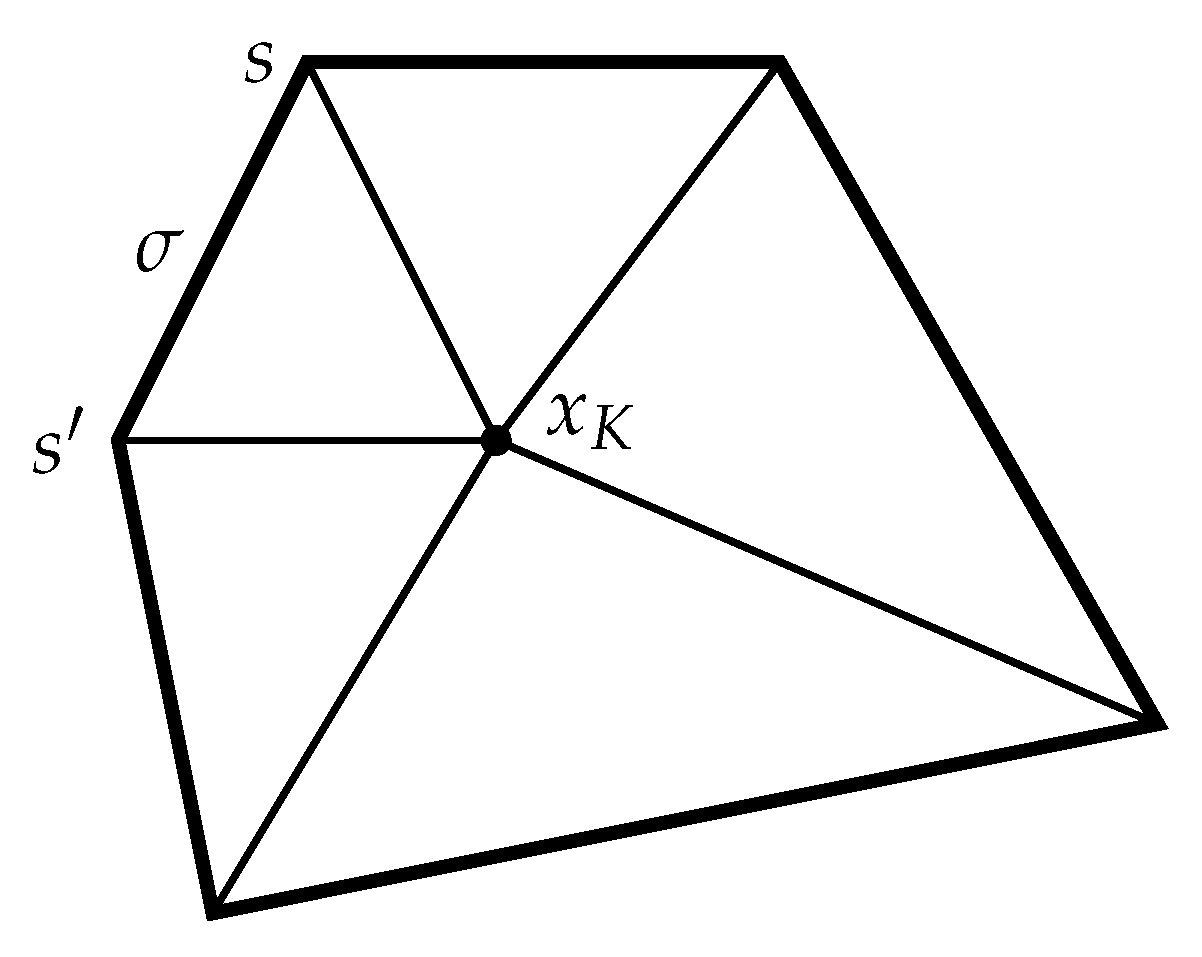
Let $\mathcal{T}$ be a mesh of $\Omega$ made up of (open, convex) disjoint polygonal cells K such that ${\cup }_{K\in \mathcal{T}}\overline{K}=\overline{\Omega }$. For all $K\in \mathcal{T}$, let $x_K\in K$ be a point such that K is star-shaped wih respect to $x_K$. We denote the set of vertices of the mesh by $\mathcal{V}$, for each $K\in \mathcal{T}$ by ${\mathcal{V}}_K$ the set of its vertices, and for each $v\in \mathcal{V}$ by ${\mathcal{T}}_K$ the set of elements containing v as a vertex.

The discrete unknowns of the VAG scheme are values at the vertices of the mesh and at the center of each element. Following [56], we define a discrete space as

$$W_{\mathcal{T}}=\left\{{\left(c_s\right)}_{s\in \mathcal{V}},{\left(c_K\right)}_{K\in \mathcal{T}},c_s=0\mathrm{for}s\in {\Gamma }_D\right\},$$

and we denote by $N_{\mathcal{T}}$ its dimension (the sum of the number of vertices and the number of cells, up to the vertices located on the Dirichlet part of the boundary).

Given a cell $K\in \mathcal{T}$, we consider the triangular submesh where, for each edge $\sigma \in {\mathcal{E}}_K$ a triangle is formed by joining the center of the cell to each of the two vertices at the ends of $\sigma$ (see Figure 1).

We can now define a discrete gradient for each discrete unknown $c_{\mathcal{T}}\in W$, as the gradient of the $P_1$ finite element function on the submesh defined above. This gradient is a constant vector on each triangular sub-cell. For future reference, we denote by ${\eta }_s,s\in \mathcal{V}$ (resp. ${\eta }_K,K\in \mathcal{T}$) the basis functions of the $P_1$ space associated to the vertices (resp. the cell centers).

The VAG scheme is defined by a variational formulation on the discrete space $W_{\mathcal{T}}$ using the gradient defined above. The gradient leads to the definition of fluxes from a cell $K\in \mathcal{T}$ to any of its vertices $v\in {\mathcal{V}}_K$. The diffusion fluxes are defined as

$$F_{K,v}^{\mathrm{d}}\left(c_{\mathcal{T}}^{n+1}\right)=\sum _{v^{\prime }\in {\mathcal{V}}_K}{T}_K^{v{v}^{\prime }}(c_K^{n+1}-c_{v^{\prime }}^{n+1}),$$

(23)

where the transmissivities $T_K^{v{v}^{\prime }}$ can be computed locally on element K. Their values are given in [56,57].

One also needs advection fluxes, defined as

$$F_{K,v}^{\mathrm{a}}\left(c_{\mathcal{T}}^{n+1}\right)=F_{K,v}^{\mathrm{d}}\left(p_{\mathcal{T}}\right)c_{K,v}^{n+1},$$

(24)

where $F_{K,v}^{\mathrm{d}}\left(p_{\mathcal{T}}\right)$ is the flux computed as in (23) with the pressure from the flow step, and $c_{K,v}$ is the upwind concentration defined as (cf [56])

$$c_{K,v}=\left\{\begin{array}{cc}{c}_K\hfill & \mathrm{if}{F}_{K,v}^{\mathrm{d}}\left(p_{\mathcal{T}}\right)\ge 0,\hfill \\ c_v\hfill & \mathrm{if}{F}_{K,v}^{\mathrm{d}}\left(p_{\mathcal{T}}\right)<0.\hfill \end{array}\right.$$

(25)

The discrete problem is now defined by the following system:

$$\left\{\begin{array}{cc}\hfill {\varphi }_K\left|K\right|{\displaystyle \frac{c_K^{n+1}{c}_K^n}{\Delta t}}+\sum _{v,v^{\prime }\in {\mathcal{V}}_K}{T}_K^{v,v^{\prime }}(c_K^{n+1}-c_{v^{\prime }}^{n+1})+\sum _{v\in {\mathcal{V}}_K}{F}_{K,v}\left(p_{\mathcal{T}}\right)c_{K,v}^{n+1}=& f_K,\forall K\in \mathcal{T}\hfill \\ \hfill {\varphi }_K\left|K\right|{\displaystyle \frac{c_v^{n+1}{c}_v^n}{\Delta t}}-\sum _{K\in {\mathcal{V}}_v,v^{\prime }\in {\mathcal{V}}_K}{T}_K^{v,v^{\prime }}(c_K^{n+1}-c_{v^{\prime }}^{n+1})-\sum _{K\in {\mathcal{T}}_v}{F}_{K,v}\left(p_{\mathcal{T}}\right)c_{K,v}^{n+1}=& f_v,\forall v\in \mathcal{V}\hfill \end{array}\right.$$

(26)

where ${\varphi }_K$ is the average porosity on cell K, $f_K={\int }_{K}f\left(x\right){\eta }_K\left(x\right)dx$ and $f_v={\int }_{\Omega }f\left(x\right){\eta }_s\left(x\right)dx$. In a more condensed notation, we have to solve a linear system

$$\mathsf{\Phi }{\displaystyle \frac{c_{\mathcal{T}}^{n+1}-c_{\mathcal{T}}^n}{\Delta t}}+A_V{c}_{\mathcal{T}}^{n+1}=f_{\mathcal{T}}^{n+1}.$$

(27)

One notes that the first equation in (26) is local to each element. The cell unkowns can thus be eliminated locally, so that the resulting system involves only the values of the concentration at the vertices. However, in a time dependent problem, the cell unknowns must be recomputed at each time step. This will be important in the coupling with the local chemical problem in Section 4.3.

With a slight abuse of notation, we denote again by ${\Psi }_T$ the discrete version of the transport operator defined in (14), so that (27) is equivalent to $c_{\mathcal{T}}^{n+1}={\Psi }_T(c_{\mathcal{T}}^n,f_{\mathcal{T}})$.

In the examples reported in Section 5, we have used ComPASS [35,58] as a black box for the transport solver. ComPASS is an open source platform for the simulation of multiphase compositional flow on generic unstructured meshes, targeting hydrothermal systems.

4.3. The Discrete Coupled Problem

We now put the two previous sections and Section 3.2 together. The framework for doing this is provided by previous work by the authors [23]. The main issue is to realize that we are solving a problem that couples all concentrations at all degrees of freedom (DOFs), both vertices and cell centers, but that transport only couples spatial DOFs while chemistry is local to each DOF. The method proposed in [22,23] attempts to decouple transport and chemistry, without sacrificing the numerical efficiency afforded by Newton’s method on the coupled problem.

The unknowns of the discrete problems are vectors in $\mathcal{X}={\mathbf{R}}^{(N_c+N_p)\times N_{\mathcal{T}}}$, and we denote them by the same letter as their continuous counterpart, written in bold face. For a vector $\mathbf{C}\in \mathcal{X}$, we follow [22] and denote by

• ${\mathbf{C}}_{:,j}$ the column vector of concentrations of all chemical species at the DOF j.
• ${\mathbf{C}}_{i,:}$ the row vector of concentrations of species i at all DOFs.

We now extend the transport and chemical operators to operate on vectors in $\mathcal{X}$.

$$\begin{array}{cc}\hfill {\Psi }_C:& \mathcal{X}\mapsto \mathcal{X}\hfill \\ & \mathbf{T}\to {\Psi }_C\left(\mathbf{T}\right),\hfill \end{array}\mathrm{and}\begin{array}{cc}\hfill {\Psi }_T:& \mathcal{X}\mapsto \mathcal{X}\hfill \\ & \mathbf{C}\to {\Psi }_C\left(\mathbf{C}\right),\hfill \end{array}$$

(28)

with

$$\begin{array}{cc}\hfill {\Psi }_C{\left(\mathbf{T}\right)}_{:,j}& ={\psi }_C\left({\mathbf{T}}_{:,j}\right),\mathrm{for}j=1,\cdots ,N_{\mathcal{T}},\hfill \\ \hfill {\Psi }_T{(\mathbf{C},\mathbf{f})}_{i,:}& ={\psi }_T({\mathbf{C}}_{i,:},{\mathbf{f}}_{i,:}),\mathrm{for}i=1,\cdots ,N_c+N_p.\hfill \end{array}$$

(29)

We also note that ${\Psi }_T$ can be made explicit, in matrix form, by making use of the Kronecker product [59]. As first explained in [21] the action of the transport operator

$${\mathbf{C}}^{n+1}={\Psi }_T({\mathbf{C}}^n,{\mathbf{f}}^{n+1})$$

is equivalent to the solution of the linear system

$$(\mathsf{\Phi }\otimes I){\displaystyle \frac{{\mathbf{C}}^{n+1}-{\mathbf{C}}^n}{\Delta t}}+(A_V\otimes I){\mathbf{C}}^{n+1}={\mathbf{f}}^{n+1}.$$

Of course the Kronecker product is just a notational device, the full matrix $A_V\otimes I$ is never actually formed. Rather, the implementation of the transport operator is done with a loop over all species, in which one time step of a transport problem is solved (see [23] for details). Similarly, the chemical solution operator ${\Psi }_C$ can be evaluated independently for each degree of freedom of the mesh.

We noted in Section 3.2 that the implementation of the Newton–Krylov method required the solution of a linear system with the jacobian of the function F defined in (16). We emphasize that this function is defined implicitly through the evaluation of both solution operators ${\Psi }_C$ and ${\Psi }_T$. Alternatively, evaluating F requires the solution of

• One step of a transport problem for each chemical species;
• One chemical equilibrium problem for each vertex and each cell.

As explained above, computing the Jacobian matrix is impractical, as it requires the inverse of the two solution operators. However, GMRES does not need the Jacobian matrix itslef, but only its action on a vector. The product $Jv$ is interpreted as a directional deritvative. We have shown in [23] how to compute this matrix vector product from the Jacobians of the transport operator (in our case, this is a linear operator) and and the chemical equilibrium operator (where the local Jacobian is needed as part of an inner Newton loop).

In this work, we have resorted to a Jacobian free version of the Newton–Krylov method (see [24] or [25,26,27]), where the required matrix by vector product is approximated bya finite difference quotient. For a small value of $\delta$ (see [46] for guidelines on how to choose $\delta$), there holds:

$$Jv=F^{\prime }\left(\overline{C}{}^{(n+1,k)}\right)v\approx {\displaystyle \frac{F(\overline{C}{}^{(n+1,k)}+\delta v)-F\left(\overline{C}{}^{(n+1,k)}\right)}{\delta }}.$$

The consequence is that the overall method can be implemented as soon as one can evaluate the transport and chemistry operators. Not only is this a mininal requirement, it is also what is needed to implement the more common Standard Iterative Approach recalled in (17). The tradeoff between both methods is an expected reduction in the number of iterations versus an increase in function evaluations for solving the linear systems at each Newton step (but notice that the Newton–Krylov methods are a special case of Inexact Newton methods, so that the linear system can be solved with an accuracy that depends on the progress of the outer Newton loop).

5. Numerical Results

5.1. Validation Example for the Interior Point Method: The Iron Precipitation Diagram

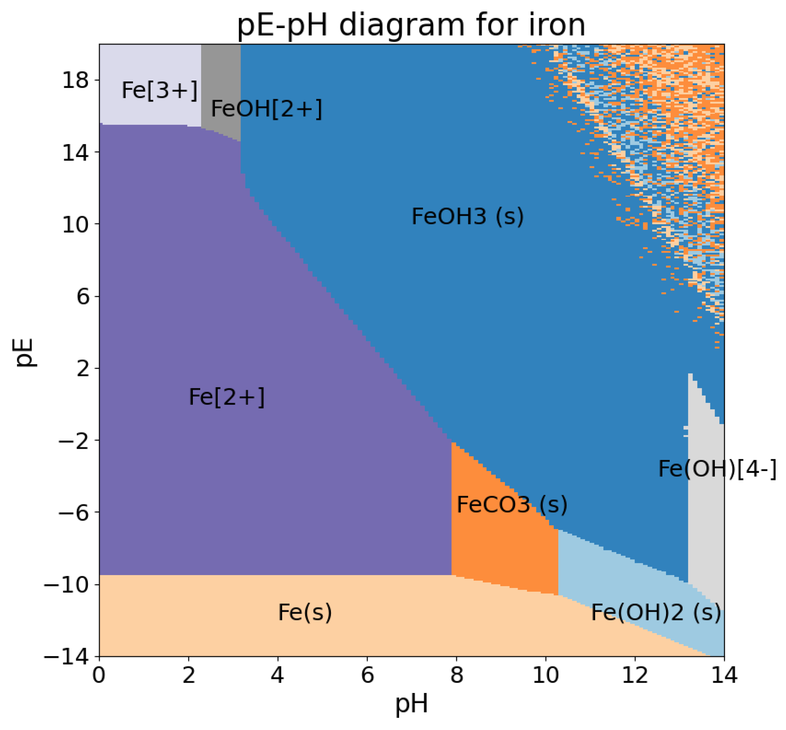
As a validation for the Newton–interior point method for computing chemical equilibrium in the presence of precipitation, we chose to recompute the pE–pH diagram for iron, also known as a Eh–pH or Pourbaix diagram ([60], p. 73).

The precise set of species used and the value of the equilibrium constants can be found in the PhD. thesis by Carrayrou [61]. It comprises nine aqueous species and four solid species.

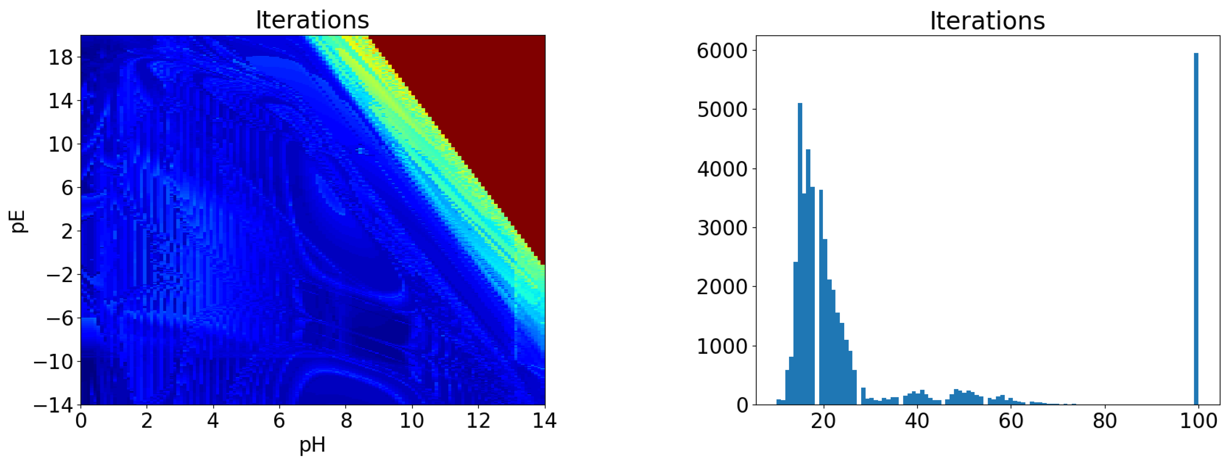
For each pair of values of the pH (between 0 and 14) and the pE (between −14 and 20), a chemical equilibrium is solved by the method detailed in Section 4.1. We first report on the number of iterations needed for the method to converge. On the left, Figure 2 shows a map of the number of iterations for each pE–pH pair, and on the right a histogram of the total number of iterations. Both images show that the method usually converges in less than 30 iterations (the average is 31.6 and the median is 19), but that it failed to converge in a significant number of cases, and we see from the left image that these cases correspond to the upper-right corner of the diagram, that is too large values of both pE and pH.

The diagram itself is shown on Figure 3. We see again in the upper right corner, and also on the rightmost band, that the Newton–IP method had difficulties with this range of values. However, the general shape of the computed diagram is in qualitative agreement with the expected behavior.

5.2. 2D Test Case: Example 11 of PhreeQC

5.2.1. Description of the Test Case

The following example simulates an advective transport in the presence of a cation exchanger. This example is adopted as a test case to validate our method in the two-dimensional case. Its 1D version represents the well known example 11 of PHREEQC documentation [37]. The example describes an experiment in a column whose chemical composition contains a cation exchanger.

Initially, the column contains a sodium-potassium-nitrate solution in equilibrium with the exchanger. The column is flushed along its left side with three pore volumes of a calcium chloride solution. Calcium, potassium, and sodium react to equilibrium with the exchanger at all times.

The flow and transport parameters used in this example are presented in

Table 1. Physical parameters.

Parameter	Value
Darcy Velocity ($\mathrm{m}$/$\mathrm{s}$)	$2.78\times {10}^{-6}$
Diffusion coeff ($\mathrm{m}$${}^2$/$\mathrm{s}$)	$5.56\times {10}^{-9}$
Domain dimensions ($\mathrm{m}$)	0.1 × 0.015
Mesh size ($\mathrm{m}$)	0.002 × 0.0015
Time duration (day)	1

, with some additional parameters to represent a 2D geometry. The initial and injected concentrations are listed in

Table 2. Initial and injected aqueous concentrations ($\mathrm{m}$$\mathrm{mol}$).

Comp.	${\mathit{C}}_{\mathbf{init}}$	${\mathit{C}}_{\mathbf{inflow}}$
Ca2+	0	$0.6\times {10}^{-3}$
Cl−	0	$1.2\times {10}^{-3}$
K+	$2\times {10}^{-4}$	0
Na+	$1\times {10}^{-3}$	0

. The cation exchanger capacity is $1.1\mathrm{m}\mathrm{mol}/\mathrm{L}$.

The chemical reactions for this example can be written as

$$\begin{array}{cc}\hfill {\mathrm{Na}}^{+}+{\mathrm{X}}^{-}& \rightleftarrows \mathrm{NaX}\hfill \\ \hfill {\mathrm{K}}^{+}+{\mathrm{X}}^{-}& \rightleftarrows \mathrm{KX}\hfill \end{array}$$

$$\frac{1}{2}{\mathrm{Ca}}^{2+}+{\mathrm{X}}^{-}\rightleftarrows \frac{1}{2}{\mathrm{CaX}}_2$$

KX, NaX, and CaX₂ are the complexes formed with the rock, while X indicates the ion exchange site with a charge −1. The chemical description (mass action and conservation laws) can be represented in the Morel tableau in Table 3:

Table 3. Moreal tableau for Phreeqc example.

	Ca${}^{2+}$	Na${}^{+}$	Cl${}^{-}$	K${}^{+}$	X	$\log \mathit{K}$
CaX2	1	0	0	0	2	3.4576
NaX	0	1	0	0	1	0
KX	0	0	0	1	1	0.7
Total	TCa	TNa	TCl	TK	W

Table 3. Moreal tableau for Phreeqc example.

	Ca${}^{2+}$	Na${}^{+}$	Cl${}^{-}$	K${}^{+}$	X	$\log \mathit{K}$
CaX2	1	0	0	0	2	3.4576
NaX	0	1	0	0	1	0
KX	0	0	0	1	1	0.7
Total	TCa	TNa	TCl	TK	W

where T_Ca, T_Na, T_Cl, T_K are the total aqueous concentrations and W is the total fixed concentrations (in this example W is a constant equal to $1.1\times {10}^{-3}$).

The domain is a rectangle that initially contains a solution of potassium and sodium, with CaCl₂ injected on all or part of the left boundary (the other boundary conditions are zero diffusive flux). We assume that the flow undergoes a uniform horizontal velocity.

We consider two different configurations depending on where CaCl₂ is injected on the left boundary of the domain:

1D configuration: 

The injection is made on the entire left boundary of the domain, which leads to a solution that depends only on x. This allows for a quick check of the method;

2D configuration: 

The injection is made only on a part of the left boundary of the domain, which gives rise to a genuinely two-dimensional solution.

5.2.2. Numerical Results

1D Configuration

In this case, CaCl is injected along the full left boundary, so that the concentration depend only on x. This allows for a comparison with the reference solution from the PhreeqC documentation [37].

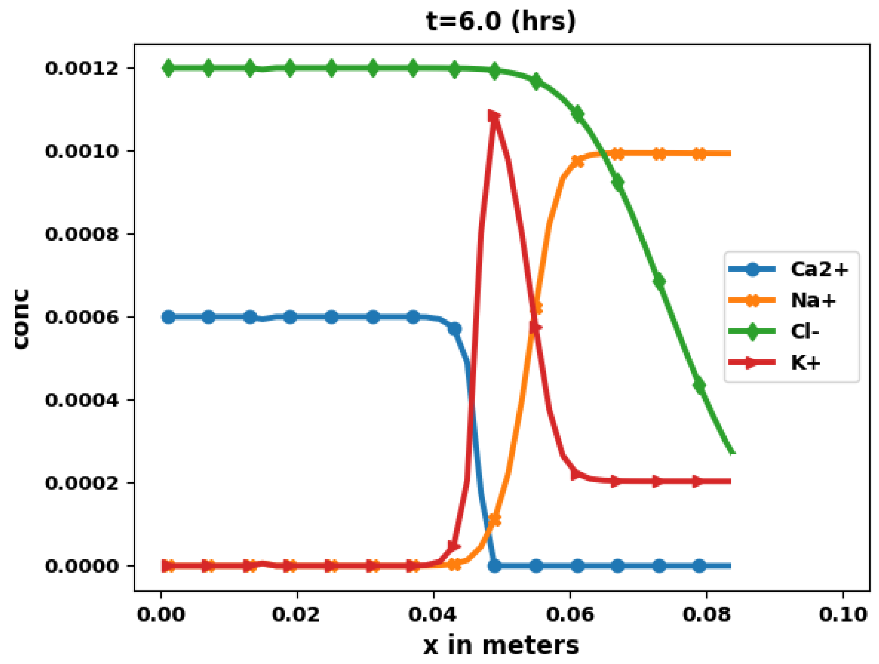
Figure 4 shows the concentrations along a horizontal line at $t=6\mathrm{h}$.

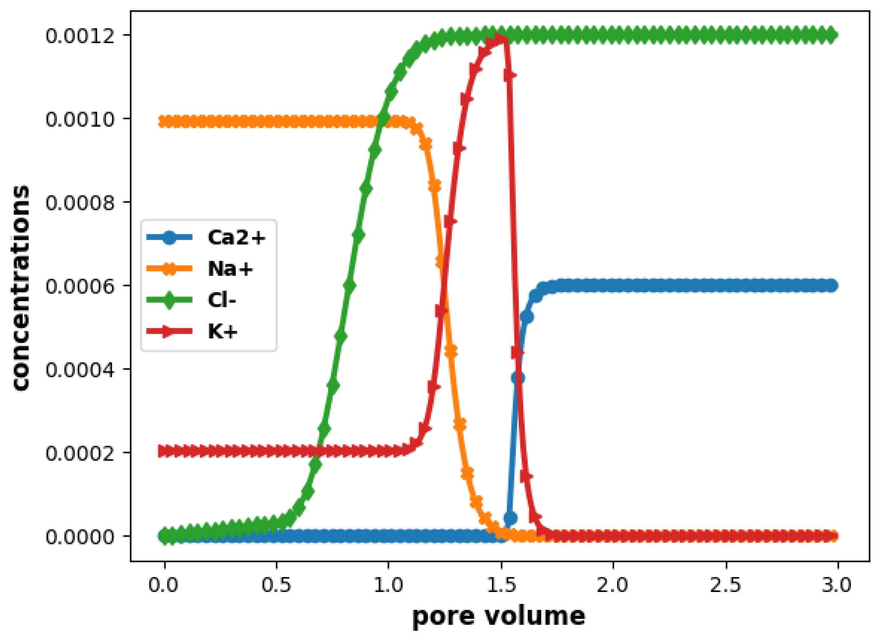
Then, we plot on Figure 5 the elution curves (concentrations at the end of the column as a function of pore volume), so as to compare with the reference solution (cf. page 241 of the PhreeqC documentation [37]). We recall that chloride is a tracer that does not react chemically, and is only subject to transport. Its concentration is given by the well known analytical solution of Ogata and Banks [62].

The results show a good agreement with those in [37].

2D Configuration

In this second case, to show real 2D effects, we inject the solution of CaCl₂ on only a part of the left boundary. We consider the same values of the concentrations at the limits, and the same initial conditions as those of the 1D configuration.

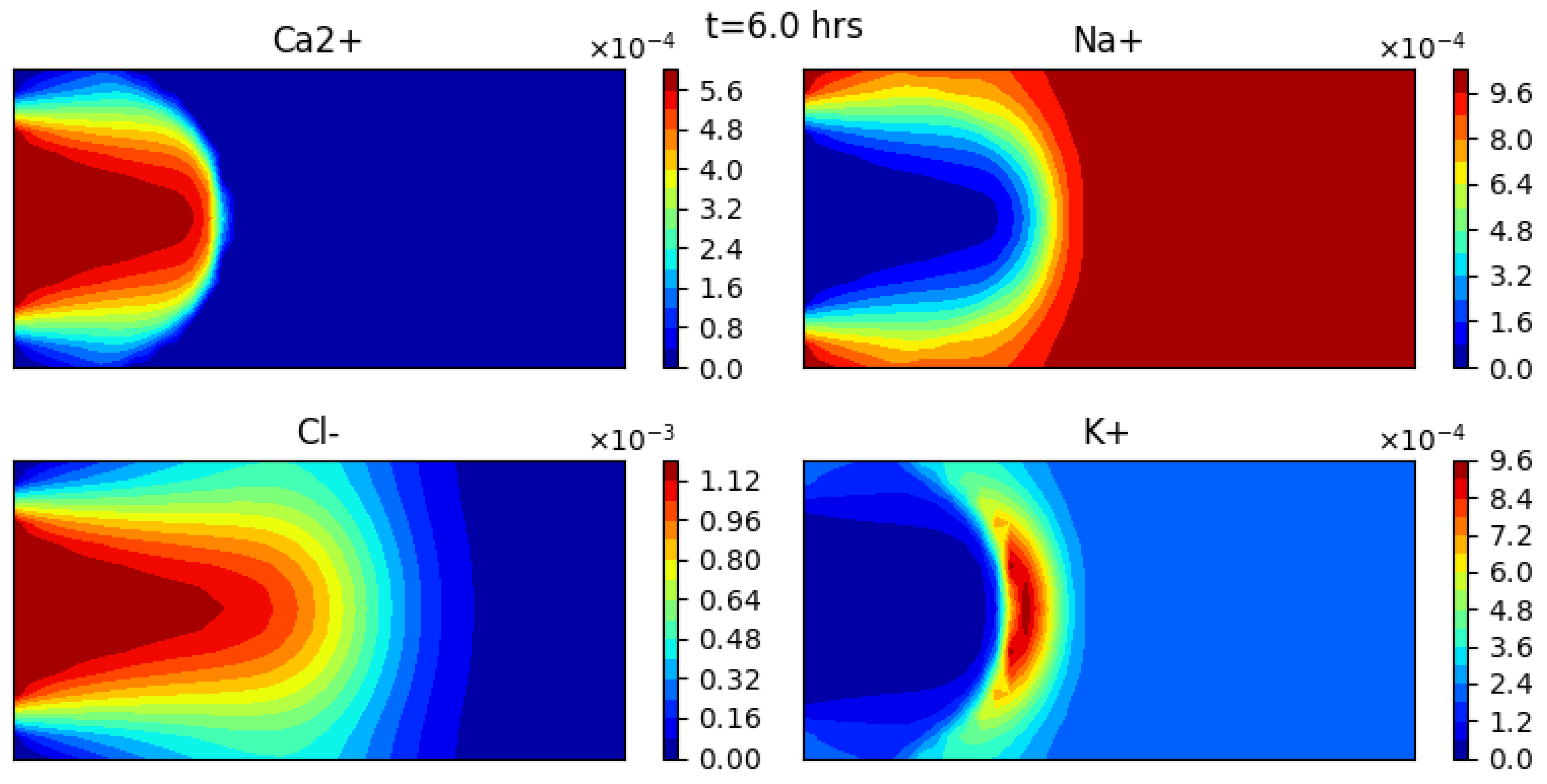
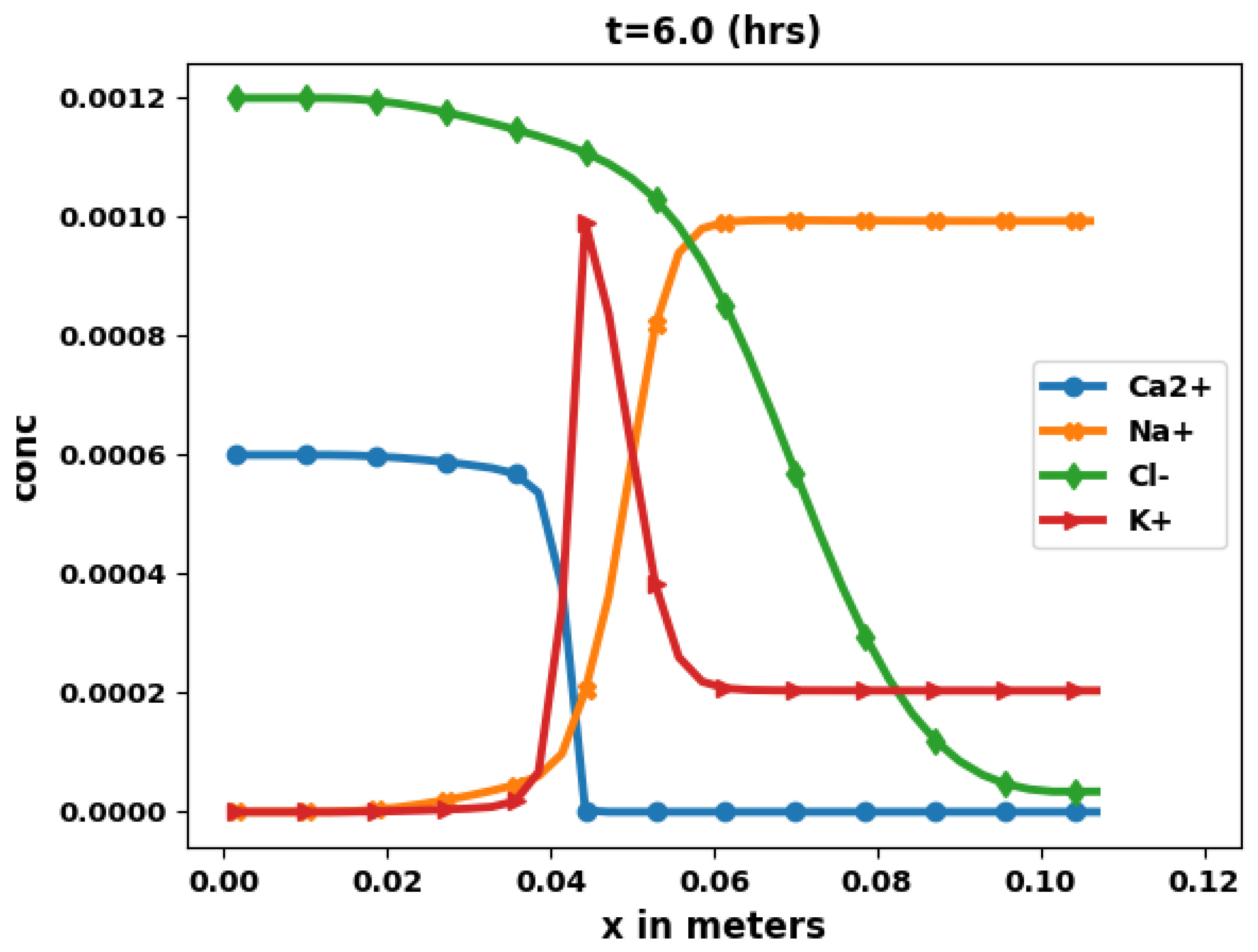
Figure 6 shows the aqueous concentration of Ca²⁺, Na⁺, Cl⁻, and K⁺, obtained at time t = 6 h, while Figure 7 shows the aqueous concentration as a function of x along the middle of the domain.

The results are consistent with physical understanding. Here also chloride remains a perfect tracer whose solution curve can be compared with an analytical solution [63]. The numerical chloride results show a good agreement with this analytical solution. The behavior of the other species is similar to the 1D case, with the addition of diffusion along the vertical direction.

5.2.3. Performance of the Elimination Method

In this section we compare the methods discussed in Section 4 for solving the coupled system: the Sequential Iterative Approach and the global approach using Newton–Krylov method (NKM in what follows), that is the nonlinear elimination strategy described in Section 3.1 and Section 4.3. Our main criterion will be the number of iterations required by each method.

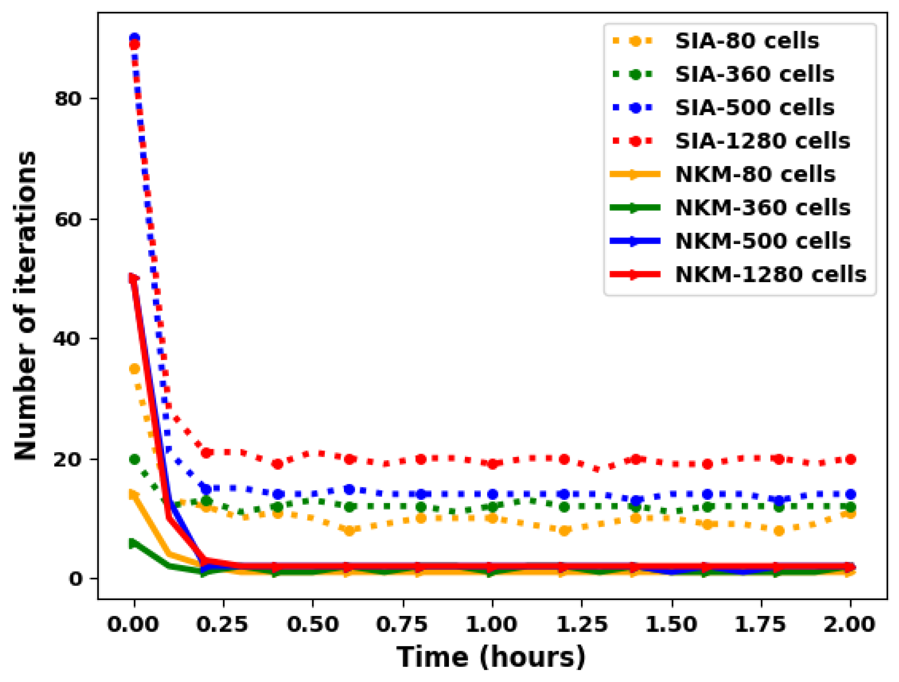
We apply the global and the splitting approaches to the 2D test case described in the previous section using several spatial resolutions (ranging from 80 to 2000 grid cells), see Figure 8.

Figure 8 shows the number of iterations required by each method per time-step for the first 20 time steps, as the mesh resolution is refined. The shape of the curves shows that the both methods have difficulty in converging for the first two time steps, but from the third time step (from time = 0.3 h), and for a given mesh resolution, the convergence becomes stable for almost the same number of iterations during the simulation.

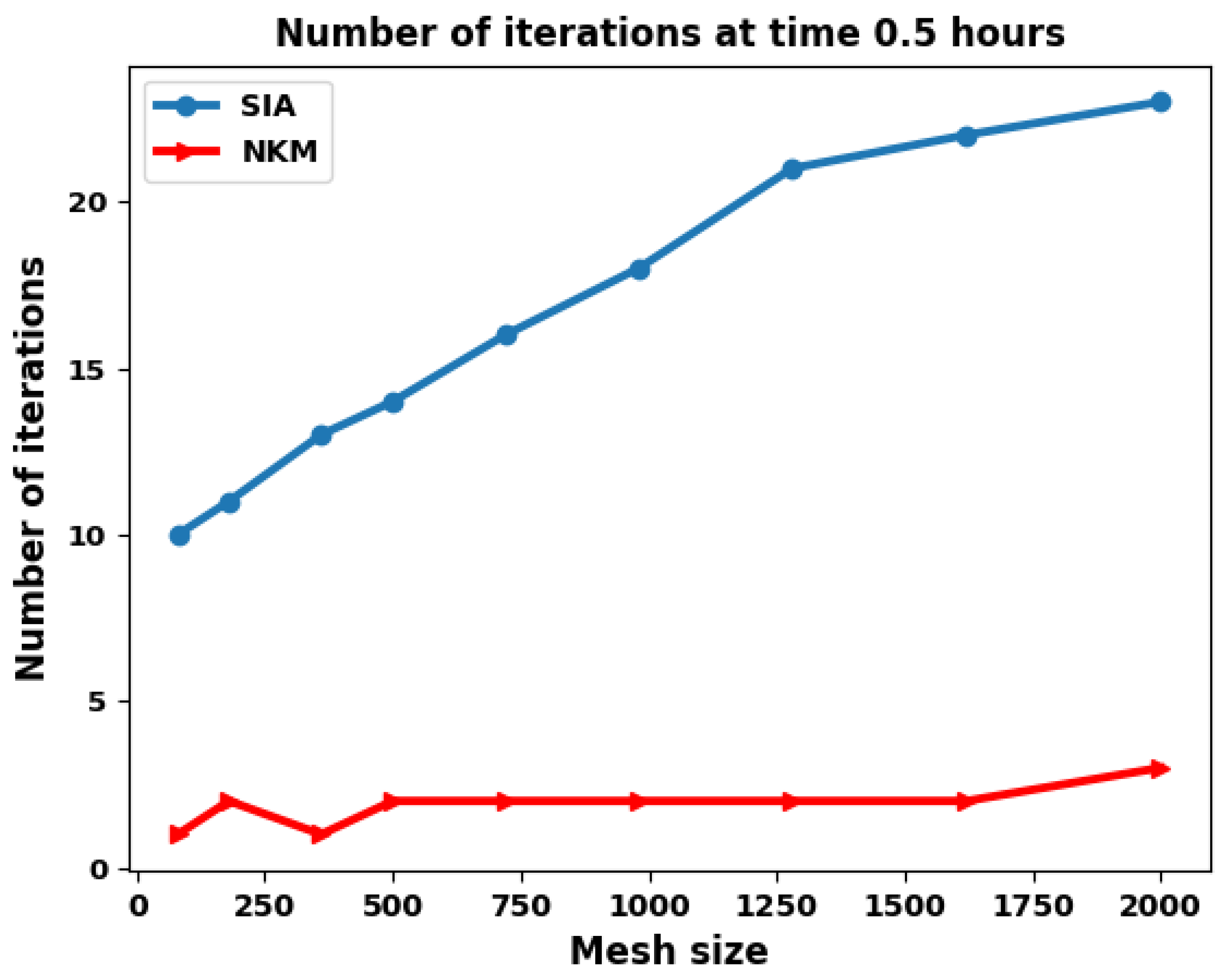
Now if we compare the two methods, SIA requires at each time step more iterations than the NKM method (the nonlinear elimination strategy). This number of iterations increases with the mesh resolution for the SIA method while it remains stable and small for the NKM method.

The NKM method requires only two nonlinear iterations on average at each time step for different mesh resolution. Figure 9 shows the results for a typical time step (at $t=0.5$ h). As predicted, the elimination method gives a convergence independent of the mesh size also in this 2D case (we had shown in [23] that this was the case for the 1D configuration).

Remark 2.

Here, we do not compare the CPU time, nor the number of evaluation of the objective function. Certainly the NKM method whose Jacobian* vector product is approximated by finite differences at each linear iteration requires a larger number of function evaluations. The number of evaluation of the function will be proportional to the number of the non-linear iterations for the NKM method times the number of GMRES iterations. We are currently investigating the use of an exact Jacobian times vector product, as this should drastically reduce the CPU time for a simulation.

5.3. SHPCO2 Benchmark

5.3.1. Description of the Test Case

The aim of this study is to test the capabilities of the equilibrium chemical solver to handle mineral precipitation and dissolution as well as taking into account chemical reactions in a spatially heterogeneous medium. The test case has been described in [64], and results can be found in [65]. The model is a simplified scenario for CO${}_2$ injection assuming the gas remain immobile, so that a one-phase flow model can be used and gaseous carbon dioxide CO₂(g) is considered as a fixed species.

The reservoir model is heterogeneous, with low permeability barriers designed to create a complex flow pattern At the same time, two injectors at different locations induce a complex mixing: one is upstream directly in contact with the bubble of CO₂ and the second one is downstream of the CO₂ bubble. At time $t=0$, supercritical CO₂(g) is injected in a specific zone and is in equilibrium with the concentrations of other chemical species.

Geometry and Physical Data

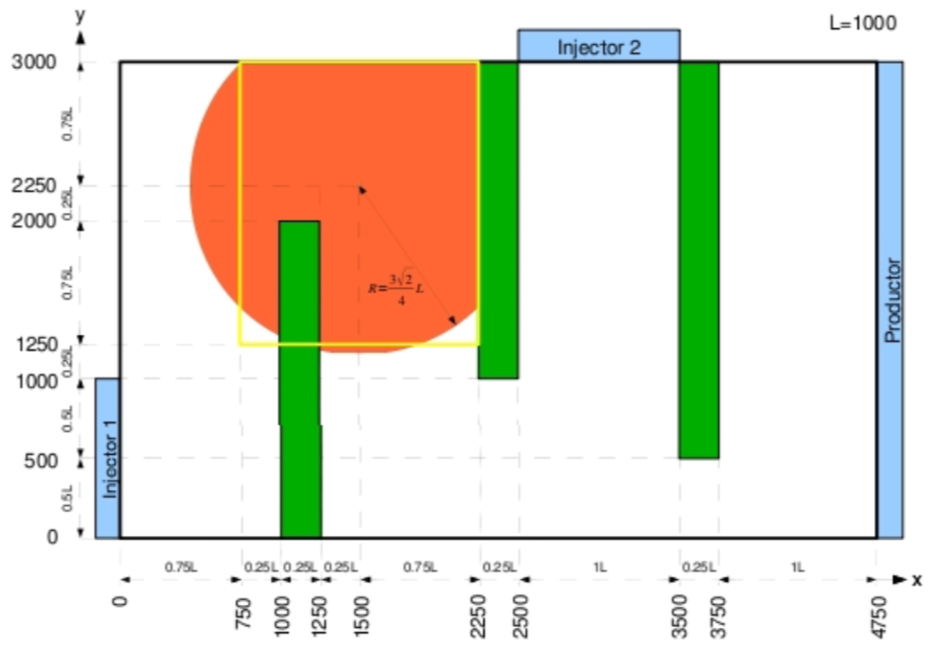
In this test we consider a two dimensional rectangular domain. A detailed geometry of the domain is shown in Figure 10. The aquifer is divided into five zones, the three green rectangle zones are low permeability barriers, the orange disc zone is the injection zone of gaseous CO₂ and has the same properties as the remaining bulk zone (in white).

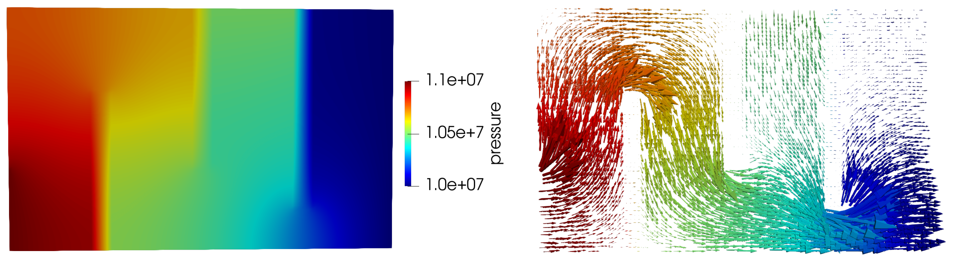
The flow in the porous medium is computed by solving a single phase flow for the Darcy velocity where the boundary conditions are 110 bars in injector 1, 105 bars in injector 2 and 110 bars in producer as labeled in Figure 10. The other boundary conditions are no flow, an impermeable Neumann boundary conditions.

The values of the flow parameters are given in

Table 4. Flow parameters.

Constants	Bulk	Barriers
Permeability K $[{\mathrm{m}}^2/\mathrm{Pa}\mathrm{s}]$	${10}^{-10}$	${10}^{-12}$
Diffusion coefficient D $[\mathrm{m}/{\mathrm{s}}^2]$	${10}^{-9}$	${10}^{-9}$
Porosity $\varphi$	0.2	0.2

. Figure 11 shows the pressure and the velocity fields, and one can see clearly the effect of the low permeability barriers.

Chemical System

The chemical system in this test consists of eight components:

• Five liquid primary components: water (H₂O), hydrogen ion (H⁺), carbon dioxide dissolved in water (CO₂(l)), calcium ion (Ca²⁺), chlorine (Cl⁻);
• Two secondary liquid components: hydroxide ion (OH⁻), hydrogen carbonate (HCO₃⁻);
• One fixed precipitated component: calcite (CaCO₃);
• One gas component: gaseous carbon dioxide (CO₂(g)).

In this test, we make the assumption that the gas phase is immobile and therefore gaseous carbon dioxide CO₂(g) can be considered like a fixed precipitated component, and because pressure variations are small throughout the domain, the partial pressure can be incorporated in the equilibrium constant for CO${}_2$ dissolution.

Among the components of the system there are four chemical reactions:

• Two aqueous equilibrium reactions:

  $$\begin{array}{cc}\hfill {\mathrm{OH}}^{-}\rightleftarrows & {\mathrm{H}}_2\mathrm{O}-{\mathrm{H}}^{+}\hfill \\ \hfill {{\mathrm{HCO}}_3}^{-}\rightleftarrows & {\mathrm{H}}_2\mathrm{O}-{\mathrm{H}}^{+}{\mathrm{H}}_2\mathrm{O}-{\mathrm{H}}^{+}+{\mathrm{CO}}_2\left(\mathrm{l}\right)\hfill \end{array}$$
• Two precipitation–dissolution reactions (taken here to be at equilibrium):

  $$\begin{array}{cc}\hfill {\mathrm{CO}}_2\left(\mathrm{g}\right)\rightleftarrows & {\mathrm{CO}}_2\left(\mathrm{l}\right)\hfill \\ \hfill {\mathrm{CaCO}}_3\rightleftarrows & {\mathrm{H}}_2\mathrm{O}-2{\mathrm{H}}^{+}+{\mathrm{CO}}_2\left(\mathrm{l}\right)+{\mathrm{Ca}}^{2+}\hfill \end{array}$$

Chlorine Cl⁻ does not participate in chemical reactions and is used as tracer. Chemical description of the test can be represented in the Morel tableau in

Table 5. Morel table for SHPCO2 system

	H${}_2$O	H${}^{+}$	CO${}_2$(l)	Ca${}^{2+}$	Cl${}^{-}$	$\log \mathit{K}$
OH−	1	$-1$	0	0	0	$-13.2354$
HCO3−	1	$-1$	1	0	0	$-6.22$
CO2(g)	0	0	1	0	0	$-0.2226$
CaCO3	1	$-2$	1	1	0	$-7.7454$
Total	$T_{\begin{array}{c}\hfill {\mathrm{H}}_2\mathrm{O}\end{array}}$	$T_{\begin{array}{c}\hfill {\mathrm{H}}^{+}\end{array}}$	$T_{\begin{array}{c}\hfill {\mathrm{CO}}_2\left(\mathrm{l}\right)\end{array}}$	$T_{\begin{array}{c}\hfill {\mathrm{Ca}}^{2+}\end{array}}$	$T_{\begin{array}{c}\hfill {\mathrm{Cl}}^{-}\end{array}}$

. The values of equilibrium constants log K are given under the condition that we use moles as units for concentration of components.

Initial State

For the transport problem, initially in the domain we have two zones with different initial values of total concentrations. The first zone is the circular area containing gaseous CO${}_2$ (in orange on Figure 10). In the rest of the domain, concentration of CO₂(g) is initially equal to zero. The initial concentrations of liquid primary components are given in

Table 6. Initial total concentrations for the SHPCO2 Benchmark.

Components	${\mathit{T}}_{\mathbf{init},\mathbf{out}\mathbf{of}\mathbf{bubble}}$ [mol/L]	${\mathit{T}}_{\mathbf{init},\mathbf{in}\mathbf{bubble}}$ [mol/L]
H2O	$77.19$	$77.21$
H+	$-43.36$	$-43.38$
CO2(l)	$21.68$	$24.37$
Ca2+	$21.72$	$21.73$
Cl−	0	1

5.3.2. Numerical Results

For this preliminary study, we have ran the simulations over the relatively short period of 1900 years. For the results reported below, we could not obtain convergence of the Newton–Krylov method. Because they appear to be qualitatively reasonable, we have nevertheless decided to include them. More investigations are underway to improve the behavior of the NKM method in the presence of minerals, and to ascertain those results. One particular direction we are currently following is to improve the computation of the Jacobian matrix by vector product, by exploiting the known block structure of the matrix.

Evolution of Concentrations

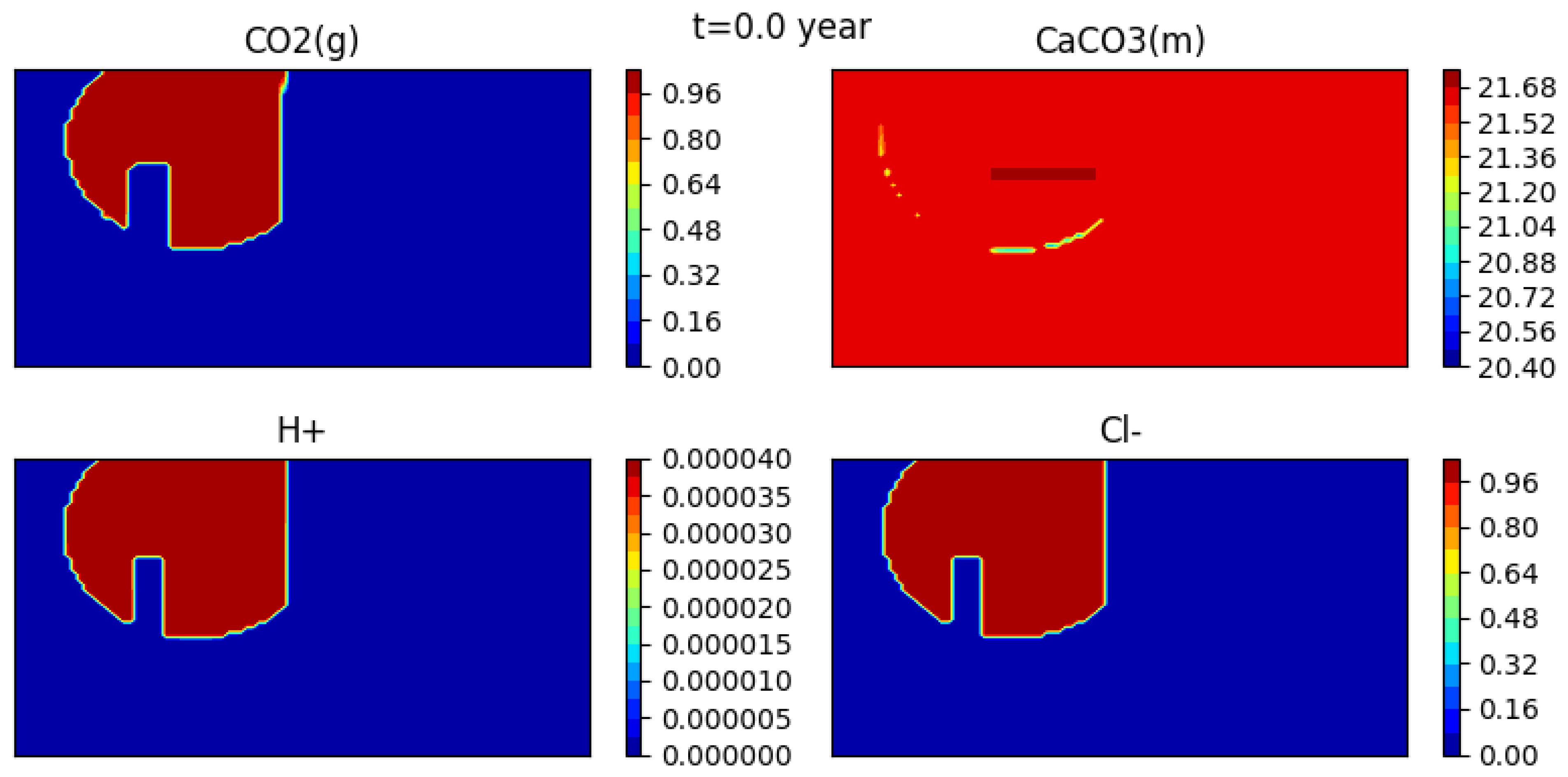
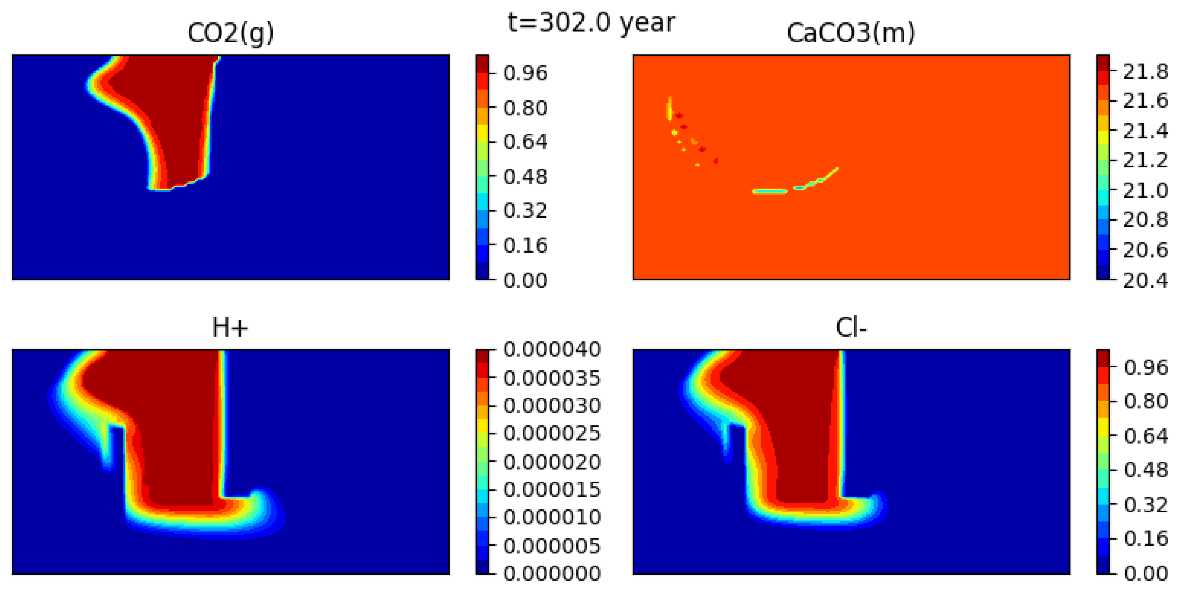
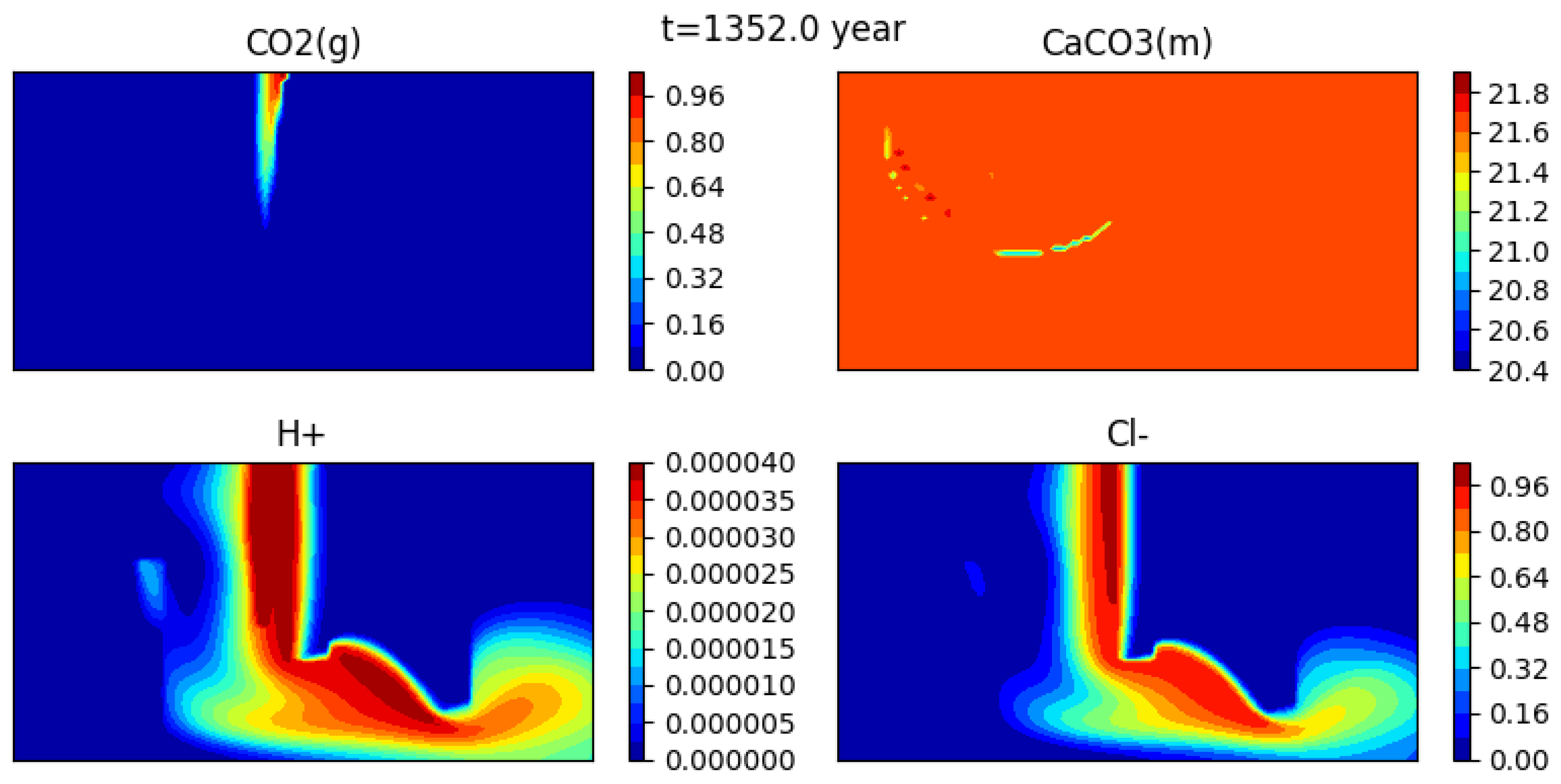
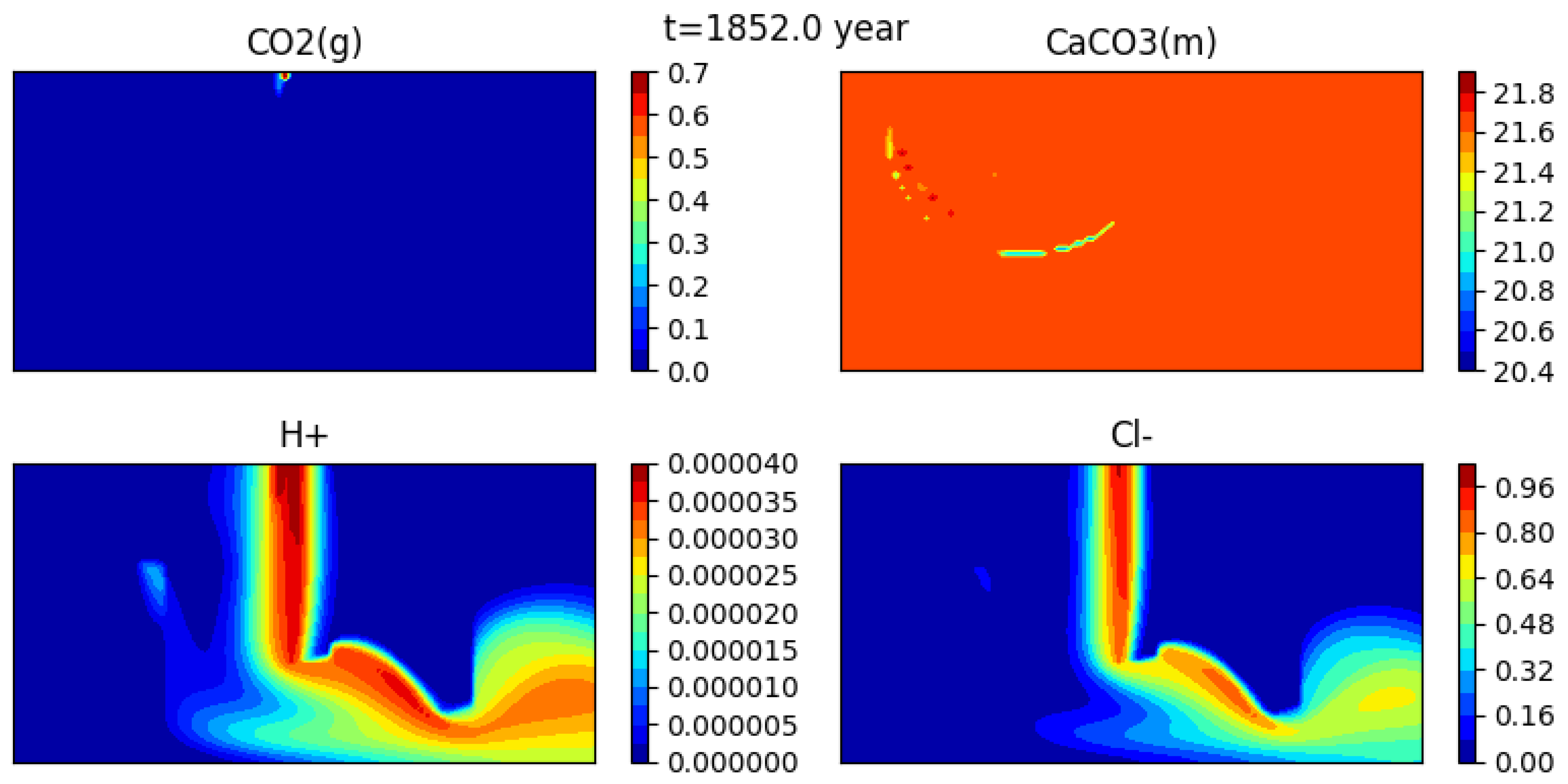
Figure 12 shows the initial condition, while Figure 13, Figure 14 and Figure 15 show snapshots of the concentrations of several species (gaseous CO${}_2$, calcite, H⁺ and CL⁻) at 302 years, 1352 years and 1852 years respectively (for a mesh with $95\times 60$ grid cells).

The gas bubble disappears as CO₂(g) dissolves into water. Here it appears that the dissolution time is somewhat less than 2000 years. At the same time, calcite precipitates, though the effect is quite small, and the medium becomes more acidic. Indeed, one can see that the concentration of H⁺ behaves somewhat differently than that of the tracer.

Variable time steps are used, as described in

Table 7. Values for variable time step simulation.

Start Time (Year)	End Time (Year)	Timestep (Year)
0	2	0.1
2	20	1
20	400	10
400	1210	50
1210	1900	100

. The time steps are chosen so as to have a small time step at the initialization when strong variations happen and to let the time step increase when the solution varies more slowly.

The results can be compared with those reported by [65]. It appears that the dissolution of the gas is faster on our simulations. On the other hand, the evolution of H⁺ happens on a similar scale as that in [65]. This is also the case for Cl⁻, as it is a tracer, and thus only subject to transport.

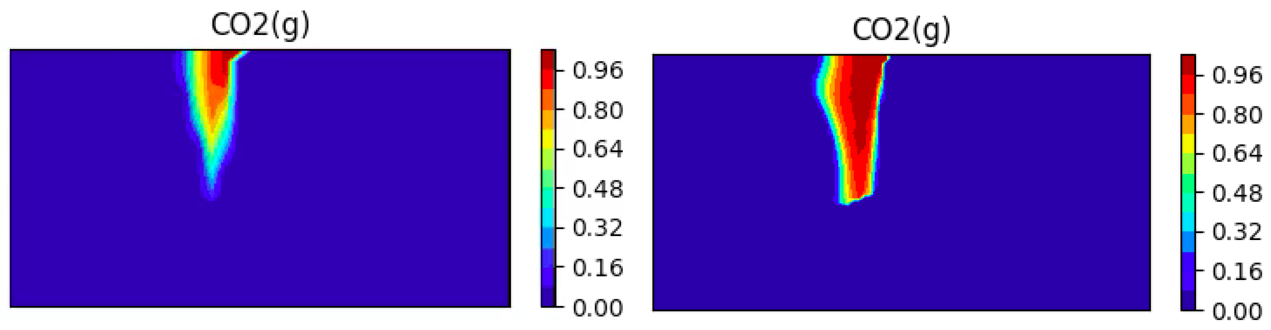
Comparison of the Dissolution CO₂(g) on Two Different Meshes

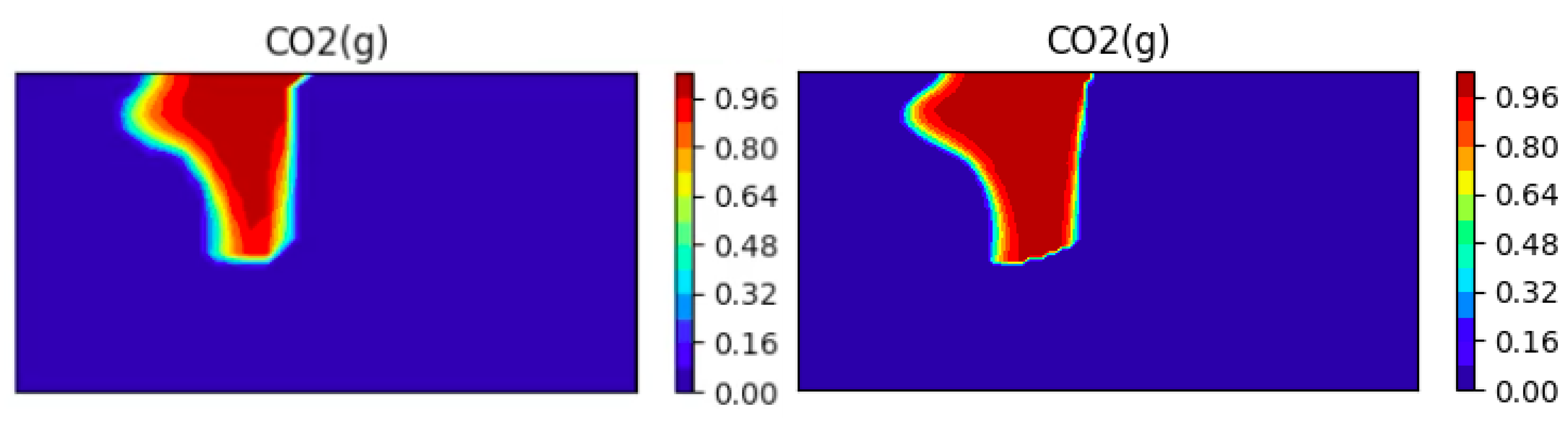
We investigate the effect of the mesh refinement on the results. We present on Figure 16 to Figure 17 the CO₂ concentrations obtained with two different meshes (a coarse mesh with $38\times 24$ cells and a fine mesh with $95\times 60$ cells) at two different times.

One can see the expected better resolution of the bubble (less numerical diffusion), but also that the speed of dissolution of the bubble changes as the mesh is refined. This is one possible explanation for the apparent shorter dissolution times that we observed as compared to [65].

References

- Zhang, F.; Yeh, G.; Parker, J. (Eds.) Groundwater Reactive Transport Models; Bentham Publishers: Sharjah, United Arab Emirates, 2012. [Google Scholar]
- Steefel, C.I.; Appelo, C.A.J.; Arora, B.; Jacques, D.; Kalbacher, T.; Kolditz, O.; Lagneau, V.; Lichtner, P.C.; Mayer, K.U.; Meeussen, J.C.L.; et al. Reactive transport codes for subsurface environmental simulation. Comput. Geosci. 2015, 19, 445–478. [Google Scholar] [CrossRef] [Green Version]
- Steefel, C.; DePaolo, D.; Lichtner, P. Reactive transport modeling: An essential tool and a new research approach for the Earth sciences. Earth Planet. Sci. Lett. 2005, 240, 539–558. [Google Scholar] [CrossRef]
- Yeh, G.T.; Tripathi, V.S. A critical evaluation of recent developments in hydrogeochemical transport models of reactive multichemical components. Water Resour. Res. 1989, 25, 93–108. [Google Scholar] [CrossRef]
- Carrayrou, J.; Mosé, R.; Behra, P. Operator-splitting procedures for reactive transport and comparison of mass balance errors. J. Contam. Hydrol. 2004, 68, 239–268. [Google Scholar] [CrossRef]
- Lagneau, V.; van der Lee, J. HYTEC results of the MoMas reactive transport benchmark. Comput. Geosci. 2010, 14, 435–449. [Google Scholar] [CrossRef] [Green Version]
- Mayer, K.U.; Frind, E.O.; Blowes, D.W. Multicomponent reactive transport modeling in variably saturated porous media using a generalized formulation for kinetically controlled reactions. Water Resour. Res. 2002, 38, 1174. [Google Scholar] [CrossRef]
- Samper, J.; Xu, T.; Yang, C. A sequential partly iterative approach for multicomponent reactive transport with CORE2D. Comput. Geosci. 2008, 13, 301–316. [Google Scholar] [CrossRef] [Green Version]
- Yeh, G.T.; Tripathi, V.S. A Model for Simulating Transport of Reactive Multispecies Components: Model Development and Demonstration. Water Resour. Res. 1991, 27, 3075–3094. [Google Scholar] [CrossRef]
- Su, D.; Mayer, K.U.; MacQuarrie, K.T.B. MIN3P-HPC: A High-Performance Unstructured Grid Code for Subsurface Flow and Reactive Transport Simulation. Math. Geosci. 2020. [Google Scholar] [CrossRef]
- Xu, T.; Sonnenthal, E.; Spycher, N.; Pruess, K. TOUGHREACT—A simulation program for non-isothermal multiphase reactive geochemical transport in variably saturated geologic media: Applications to geothermal injectivity and CO2 geological sequestration. Comput. Geosci. 2006, 32, 145–165. [Google Scholar] [CrossRef]
- Yapparova, A.; Gabellone, T.; Whitaker, F.; Kulik, D.A.; Matthäi, S.K. Reactive Transport Modelling of Dolomitisation Using the New CSMP++GEM Coupled Code: Governing Equations, Solution Method and Benchmarking Results. Transp. Porous Med. 2017, 117, 385–413. [Google Scholar] [CrossRef] [Green Version]
- Fan, Y.; Durlofsky, L.J.; Tchelepi, H.A. A fully-coupled flow-reactive-transport formulation based on element conservation, with application to CO2 storage simulations. Adv. Water Resour. 2012, 42, 47–61. [Google Scholar] [CrossRef]
- Ahusborde, E.; El Ossmani, M.; Moulay, M.I. A fully implicit finite volume scheme for single phase flow with reactive transport in porous media. Math. Comput. Simul. 2019, 164, 3–23. [Google Scholar] [CrossRef]
- Hoffmann, J.; Kräutle, S.; Knabner, P. A parallel global-implicit 2-D solver for reactive transport problems in porous media based on a reduction scheme and its application to the MoMaS benchmark problem. Comput. Geosci. 2009, 14, 421–433. [Google Scholar] [CrossRef]
- Kräutle, S.; Knabner, P. A new numerical reduction scheme for fully coupled multicomponent transport-reaction problems in porous media. Water Resour. Res. 2005, 41. [Google Scholar] [CrossRef] [Green Version]
- Kräutle, S.; Knabner, P. A reduction scheme for coupled multicomponent transport-reaction problems in porous media: Generalization to problems with heterogeneous equilibrium reactions. Water Resour. Res. 2007, 43. [Google Scholar] [CrossRef]
- de Dieuleveult, C.; Erhel, J.; Kern, M. A global strategy for solving reactive transport equations. J. Comput. Phys. 2009, 228, 6395–6410. [Google Scholar] [CrossRef]
- De Dieuleveult, C.; Erhel, J. A global approach to reactive transport: Application to the MoMas benchmark. Comput. Geosci. 2010, 14, 451–464. [Google Scholar] [CrossRef] [Green Version]
- Erhel, J.; Sabit, S. Analysis of a Global Reactive Transport Model and Results for the MoMaS Benchmark. Math. Comput. Simul. 2017, 137, 286–298. [Google Scholar] [CrossRef] [Green Version]
- Erhel, J.; Sabit, S.; de Dieuleveult, C. Solving Partial Differential Algebraic Equations and Reactive Transport Models. In Developments in Parallel, Distributed, Grid and Cloud Computing for Engineering; Topping, B.H.V., Ivànyi, P., Eds.; Computational Science, Engineering and Technology Series; Saxe Coburg Publications: London, UK, 2013; pp. 151–169. [Google Scholar]
- Amir, L.; Kern, M. A global method for coupling transport with chemistry in heterogeneous porous media. Comput. Geosci. 2010, 14, 465–481. [Google Scholar] [CrossRef] [Green Version]
- Amir, L.; Kern, M. Preconditioning a Coupled Model for Reactive Transport in Porous Media. Int. J. Numer. Anal. Model. 2019, 16, 18–48. [Google Scholar]
- Knoll, D.A.; Keyes, D.E. Jacobian-free Newton-Krylov methods: A survey of approaches and applications. J. Comput. Phys. 2004, 193, 357–397. [Google Scholar] [CrossRef] [Green Version]
- Hammond, G.E.; Valocchi, A.; Lichtner, P. Application of Jacobian-free Newton–Krylov with physics-based preconditioning to biogeochemical transport. Adv. Water Resour. 2005, 28, 359–376. [Google Scholar] [CrossRef]
- Carr, E.; Turner, I.; Perré, P. A variable-stepsize Jacobian-free exponential integrator for simulating transport in heterogeneous porous media: Application to wood drying. J. Comput. Phys. 2013, 233, 66–82. [Google Scholar] [CrossRef]
- Guo, L.; Huang, H.; Gaston, D.R.; Permann, C.J.; Andrs, D.; Redden, G.D.; Lu, C.; Fox, D.T.; Fujita, Y. A parallel, fully coupled, fully implicit solution to reactive transport in porous media using the preconditioned Jacobian-Free Newton-Krylov Method. Adv. Water Resour. 2013, 53, 101–108. [Google Scholar] [CrossRef]
- Kräutle, S. The semismooth Newton method for multicomponent reactive transport with minerals. Adv. Water Resour. 2011, 34, 137–151. [Google Scholar] [CrossRef]
- Buchholzer, H.; Kanzow, C.; Knabner, P.; Kräutle, S. The semismooth Newton method for the solution of reactive transport problems including mineral precipitation-dissolution reactions. Comput. Optim. Appl. 2011, 50, 193–221. [Google Scholar] [CrossRef] [Green Version]
- Kräutle, S. Existence of global solutions of multicomponent reactive transport problems with mass action kinetics in porous media. J. Appl. Anal. Comput. 2011, 1, 497–515. [Google Scholar]
- El-Bakry, A.S.; Tapia, R.A.; Tsuchiya, T.; Zhang, Y. On the formulation and theory of the Newton interior-point method for nonlinear programming. J. Optim. Theory Appl. 1996, 89, 507–541. [Google Scholar] [CrossRef]
- Leal, A.M.M.; Kulik, D.A.; Smith, W.R.; Saar, M.O. An overview of computational methods for chemical equilibrium and kinetic calculations for geochemical and reactive transport modeling. Pure Appl. Chem. 2017, 89, 597–643. [Google Scholar] [CrossRef]
- Saaf, F.E. A Study of Reactive Transport Phenomena in Porous Media. Ph.D. Thesis, Rice University, Houston, TX, USA, 1997. [Google Scholar]
- Arbogast, T.; Bryant, S.; Dawson, C.; Saaf, F.; Wang, C.; Wheeler, M. Computational methods for multiphase flow and reactive transport problems arising in subsurface contaminant remediation. J. Comput. Appl. Math. 1996, 74, 19–32. [Google Scholar] [CrossRef] [Green Version]
- Lopez, S.; Masson, R.; Beaude, L.; Birgle, N.; Brenner, K.; Kern, M.; Smaï, F.; Xing, F. Geothermal Modeling in Complex Geological Systems with the ComPASS Code. In Stanford Geothermal Workshop 2018—43rd Workshop on Geothermal Reservoir Engineering; Stanford University: Stanford, CA, USA, 2018. [Google Scholar]
- Eymard, R.; Guichard, C.; Herbin, R. Small-stencil 3D schemes for diffusive flows in porous media. ESAIM Math. Model. Numer. Anal. 2012, 46, 265–290. [Google Scholar] [CrossRef] [Green Version]
- Parkhurst, D.L.; Appelo, C. User’s Guide to PHREEQC (Version 2)—A Computer Program for Speciation, Batch-Reaction, One-Dimensional Transport, and Inverse Geochemical Calculations; Technical Report 99-4259; USGS: Reston, VA, USA, 1999. [Google Scholar]
- Appelo, C.A.J.; Postma, D. Geochemistry, Groundwater and Pollution, 2nd ed.; CRC Press: Boca Raton, FL, USA, 2005. [Google Scholar]
- Rubin, J. Transport of reacting Solutes in Porous Media: Relation Between Mathematical Nature of Problem Formulation and Chemical Nature of reactions. Water Resour. Res. 1983, 19, 1231–1252. [Google Scholar] [CrossRef]
- Bear, J.; Cheng, A.H.D. Modeling Groundwater Flow and Contaminant Transport; Theory and Applications of Transport in Porous Media; Springer: Berlin/Heidelberg, Germany, 2010; Volume 23. [Google Scholar]
- Saaltink, M.; Ayora, C.; Carrera, J. A Mathematical Formulation for Reactive Transport that Eliminates Mineral Concentrations. Water Resour. Res. 1998, 34, 1649–1656. [Google Scholar] [CrossRef]
- Fahs, M.; Carrayrou, J.; Younes, A.; Ackerer, P. On the efficiency of the direct substitution approach for reactive transport problems in porous media. Water Air Soil Pollut. 2008, 193, 299–308. [Google Scholar] [CrossRef]
- Saaltink, M.; Carrera, J.; Ayora, C. On the behavior of approaches to simulate reactive transport. J. Contam. Hydrol. 2001, 48, 213–235. [Google Scholar] [CrossRef]
- Kanney, J.F.; Miller, C.T.; Kelley, C.T. Convergence of Iterative Split Operator Approaches for Approximating Nonlinear Reactive Transport Problems. Adv. Water Resour. 2003, 26, 247–261. [Google Scholar] [CrossRef] [Green Version]
- Saaltink, M.; Carrera, J.; Ayora, C. A Comparison of Two Approaches for Reactive Transport Modelling. J. Geochem. Explor. 2000, 69–70, 97–101. [Google Scholar] [CrossRef]
- Kelley, C.T. Iterative Methods for Linear and Nonlinear Equations; With Separately Available Software, Frontiers in Applied Mathematics; SIAM: Philadelphia, PA, USA, 1995; Volume 16, pp. 154–165. [Google Scholar]
- Saad, Y.; Schultz, M.H. GMRES: A generalized minimal residual algorithm for solving nonsymmetric linear systems. SIAM J. Sci. Stat. Comput. 1986, 7, 856–869. [Google Scholar] [CrossRef] [Green Version]
- Hoffmann, J.; Kräutle, S.; Knabner, P. A general reduction scheme for reactive transport in porous media. Comput. Geosci. 2012, 16, 1081–1099. [Google Scholar] [CrossRef]
- Marinoni, M.; Carrayrou, J.; Lucas, Y.; Ackerer, P. Thermodynamic Equilibrium Solutions Through a Modified Newton Raphson Method. AIChE J. 2016, 63, 1246–1262. [Google Scholar] [CrossRef]
- Wolery, T.; Jarek, R.L. Software User’s Manual; EQ3/6, Version 8.0; Sandia National Laboratories: Albuquerque, Bernalillo, 2003. [Google Scholar]
- Facchinei, F.; Pang, J.S. Finite-Dimensional Variational Inequalities and Complementarity Problems; Springer Series in Operations Research; Springer: New York, NY, USA, 2003; Volume I, pp. 34, 624, I69. [Google Scholar]
- Facchinei, F.; Pang, J.S. Finite-Dimensional Variational Inequalities and Complementarity Problems; Springer Series in Operations Research; Springer: New York, NY, USA, 2003; Volume II, pp. 1–34, 625–1234, II1–II57. [Google Scholar]
- Bethke, C.M. Geochemical and Biogeochemical Reaction Modeling, 2nd ed.; Cambridge University Press: Cambridge, UK, 2008. [Google Scholar]
- Carrayrou, J. Looking for some reference solutions for the reactive transport benchmark of MoMaS with SPECY. Comput. Geosci. 2010. [Google Scholar] [CrossRef]
- Leal, A.M.; Blunt, M.J.; LaForce, T.C. Efficient chemical equilibrium calculations for geochemical speciation and reactive transport modelling. Geochim. Cosmochim. Acta 2014, 131, 301–322. [Google Scholar] [CrossRef] [Green Version]
- Eymard, R.; Guichard, C.; Herbin, R.; Masson, R. Vertex centred discretization of two-phase Darcy flows on general meshes. In Congrès National de Mathématiques Appliquées et Industrielles; ESAIM Proc.; EDP Sciences: Les Ulis, France, 2011; Volume 35, pp. 59–78. [Google Scholar] [CrossRef]
- Eymard, R.; Guichard, C.; Herbin, R.; Masson, R. Vertex-centred discretization of multiphase compositional Darcy flows on general meshes. Comput. Geosci. 2012, 16, 987–1005. [Google Scholar] [CrossRef] [Green Version]
- Dalissier, E.; Guichard, C.; Havé, P.; Masson, R.; Yang, C. ComPASS: A tool for distributed parallel finite volume discretizations on general unstructured polyhedral meshes. In CEMRACS 2012; ESAIM Proc.; EDP Sciences: Les Ulis, France, 2013; Volume 43, pp. 147–163. [Google Scholar] [CrossRef]
- Golub, G.H.; van Loan, C.F. Matrix Computations, 4th ed.; Johns Hopkins University Press: Baltimore, MD, USA, 2013. [Google Scholar]
- Brookins, D.G. Eh-pH Diagrams for Geochemistry; Springer: Berlin/Heidelberg, Germany, 1988. [Google Scholar]
- Carrayrou, J. Modélisation du Transport de Solutes Réactifs en Milieu Poreux Saturé. Thèse de Doctorat, Université Louis Pasteur, Strasbourg, France, 2001. [Google Scholar]
- Ogata, A.; Banks, R.B. A Solution of the Differential Equation of Longitudinal Dispersion in Porous Media; Technical Report Prof. Pap., 411-A; USGS: Reston, VA, USA, 1961. [Google Scholar]
- Feike, L.; Dane, J.H. Analytical solution of the one dimensional advection equation equation and two- or tree-dimentional dispersion equation. Water Ressources Res. 1990, 26, 1475–1482. [Google Scholar]
- Haeberlein, F. Time Space Domain Decomposition Methods for Reactive Transport—Application to CO2 Geological Storage. Thèse de Doctorat, Université Paris 13, Paris, France, 2011. [Google Scholar]
- Ahusborde, E.; El Ossmani, E. A sequential approach for numerical simulation of two-phase multicomponent flow with reactive transport in porous media. Math. Comput. Simul. 2017, 137, 71–89. [Google Scholar] [CrossRef]
Figure 1.
Triangular submesh for a cell K.
Figure 2.
Number of iterations for the iron precipitation example. (Left) map as a function of pH and pE, (Right) histogram of iteration number.
Figure 3.
pH–pE diagram (Pourbaix diagram) for iron. In each region, the dominant species is shown.
Figure 4.
Total aqueous concentrations for y = 0.0075, at t = 6 h.
Figure 5.
Evolution of concentrations at the end of the column.
Figure 6.
Total aqueous concentrations at t = 6 h.
Figure 7.
Total aqueous concentrations for , at h.
Figure 8.
Number of iterations per time-step for the first 20 time-steps for the various solution methods.
Figure 9.
Number of Iterations as a function of the mesh size for the various solution methods at t = 0.5 h.
Figure 10.
Geometry of domain for the SHPCO2 Benchmark.
Figure 11.
Pressure and velocity for the SHPCO2 model.
Figure 12.
Concentrations of the gas CO2(g), the calcite CaCO3, H+ and the tracer Cl− at t = 0 year.
Figure 13.
Concentrations of the gas CO2(g), the calcite CaCO3, H+ and the tracer Cl− at t = 302 year.
Figure 14.
Concentrations of the gas CO2(g), the calcite CaCO3, H+ and the tracer Cl− at t = 1352 year.
Figure 15.
Concentrations of the gas CO2(g), the calcite CaCO3, H+ and the tracer Cl− at t = 1852 year.
Figure 16.
CO2(g), at t = 302 y (left image: coarse mesh, right image: fine mesh).
Figure 17.
CO2(g), at t = 800 y (left image: coarse mesh, right image: fine mesh).