
Flood Suspended Sediment Transport: Combined Modelling from Dilute to Hyper-Concentrated Flow

 ,
,  ,
,  , , and
Abstract
:1. Introduction
2. Models Review
3. Proposed Modelling
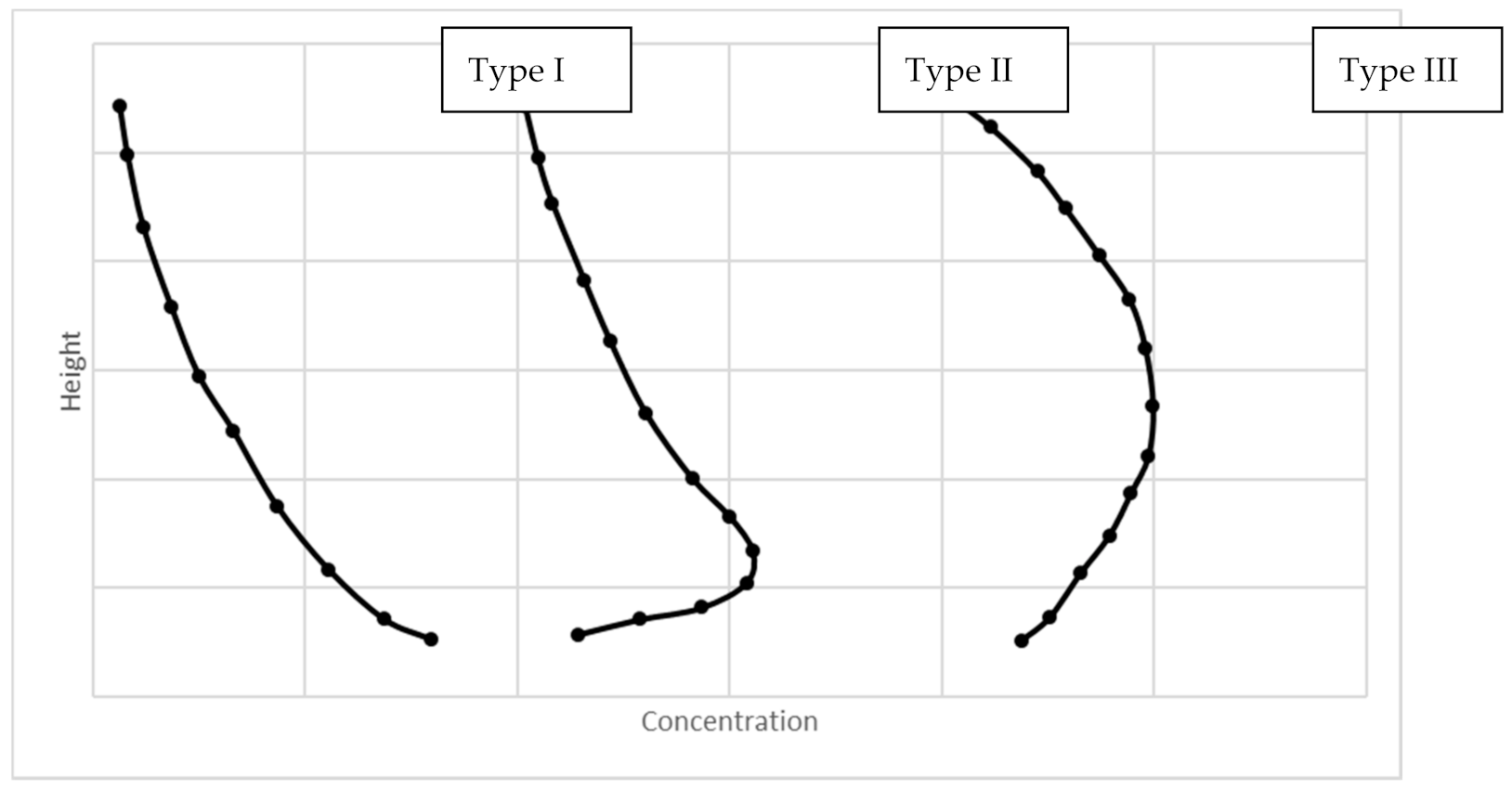
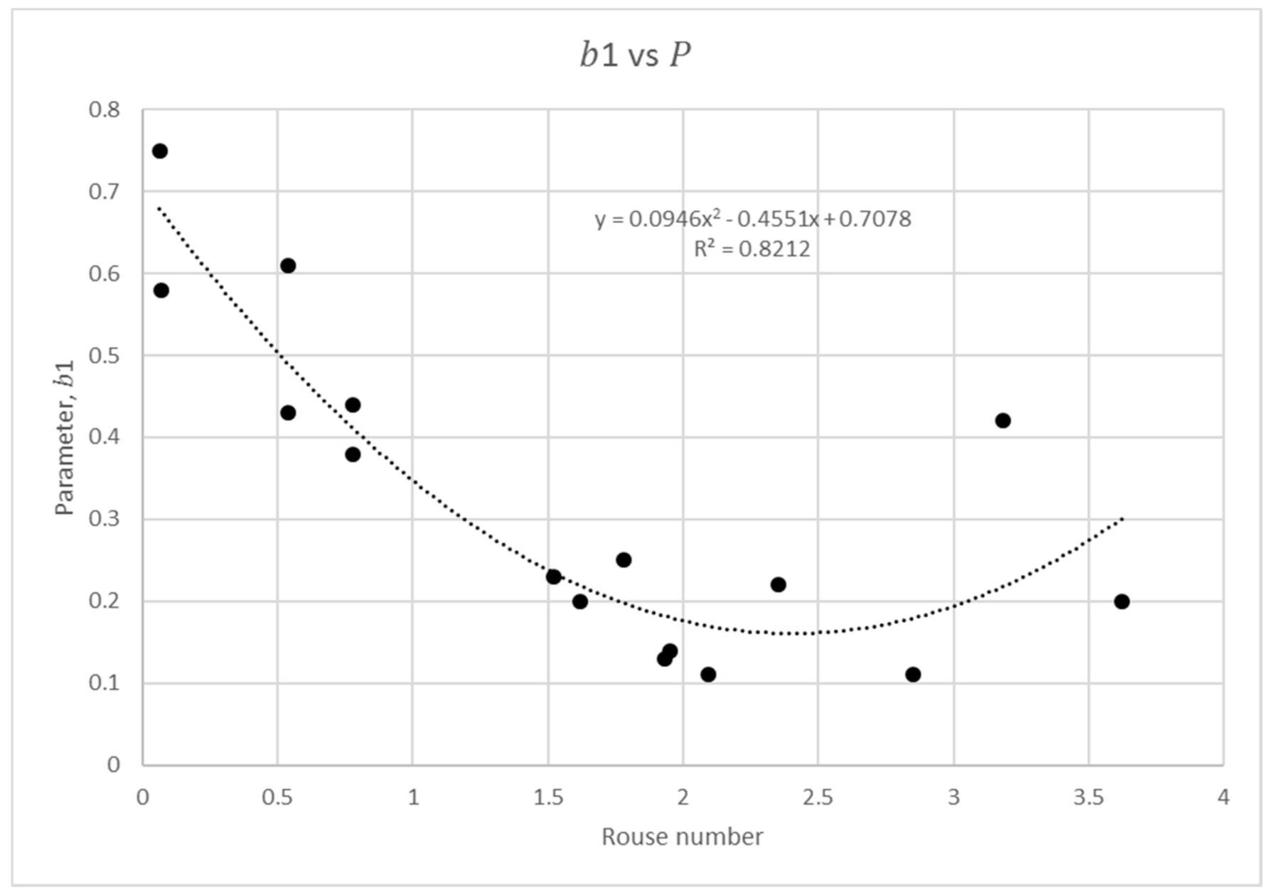
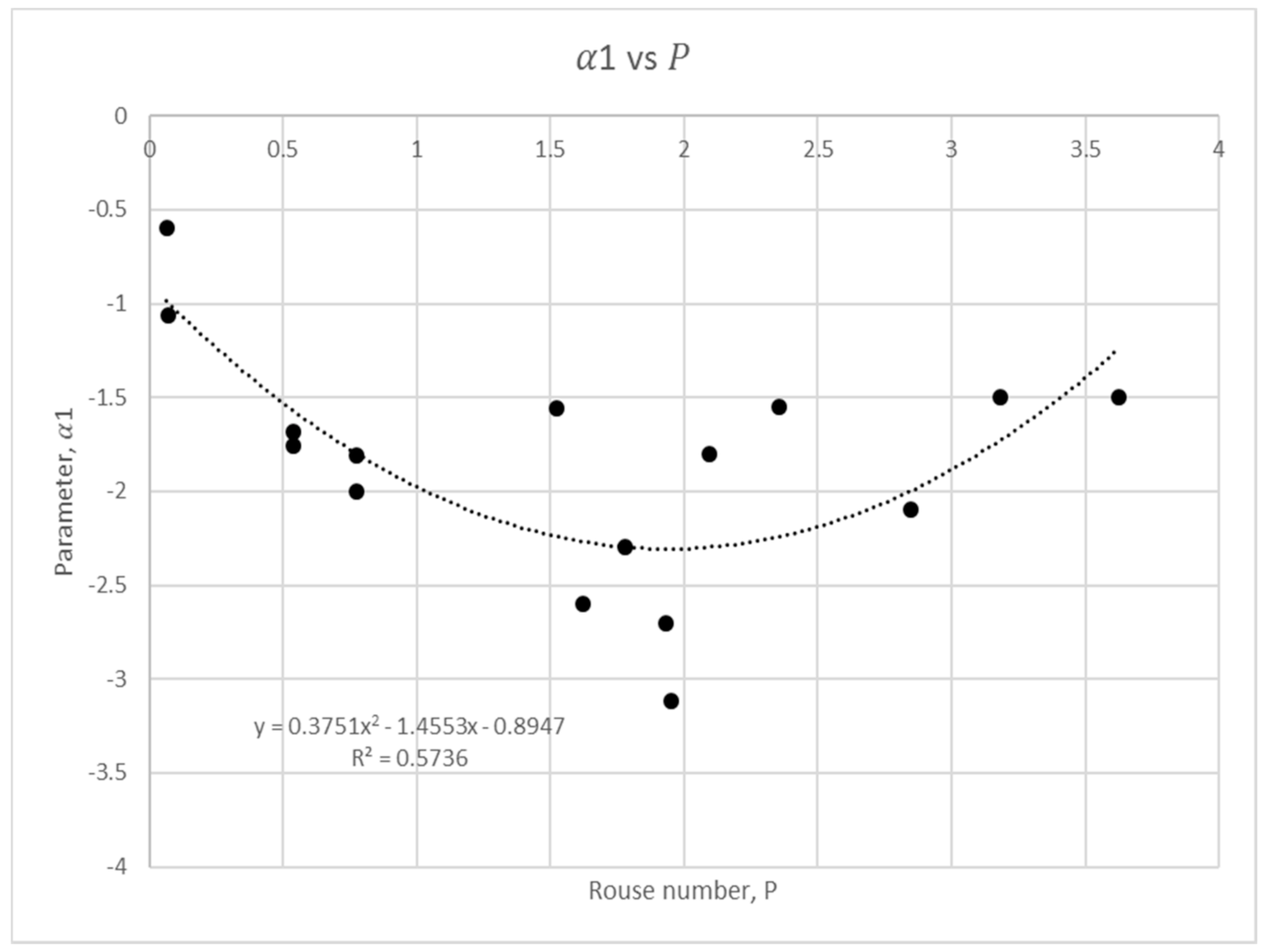
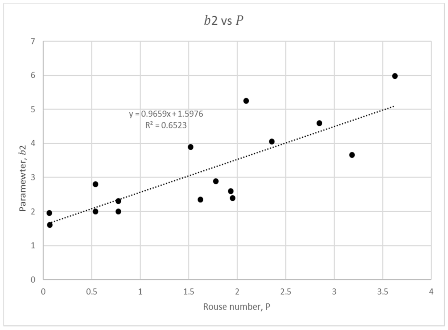
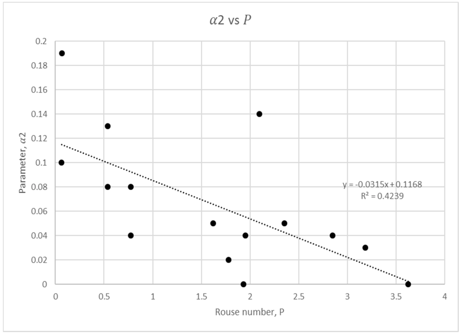
3.1. Rouse Number
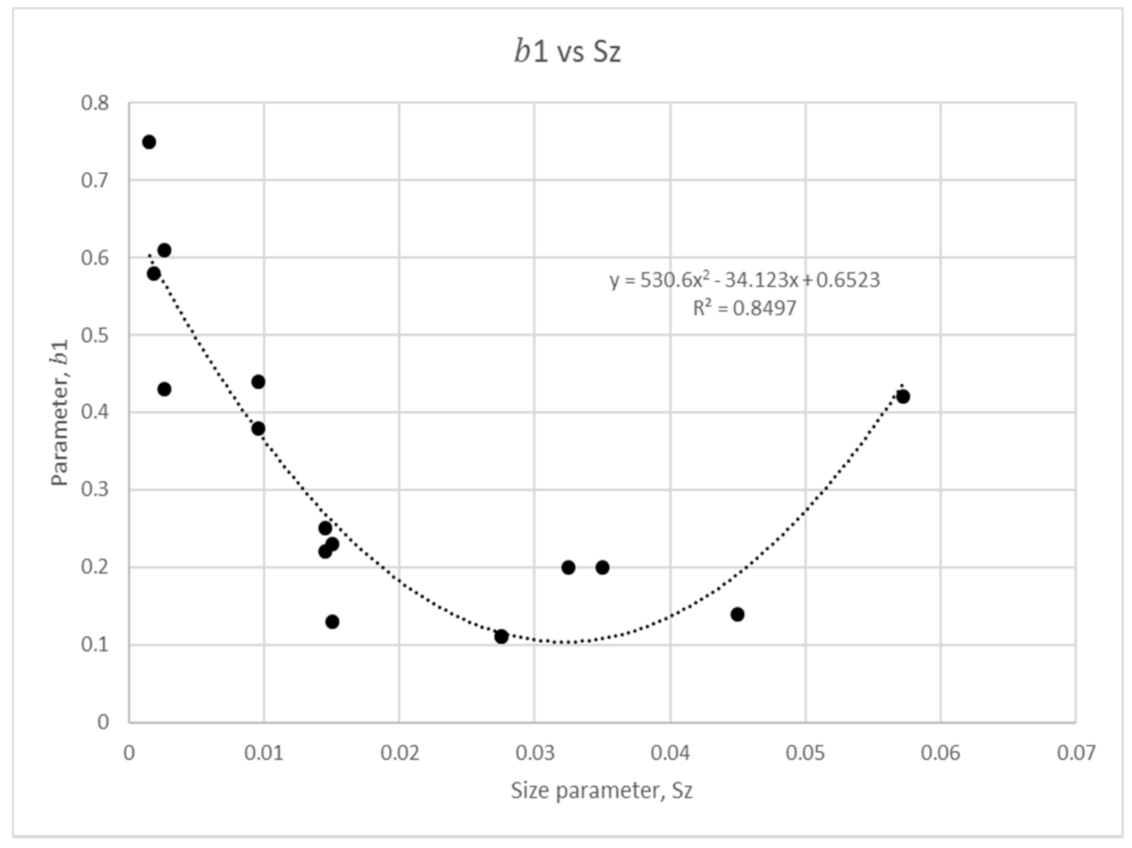
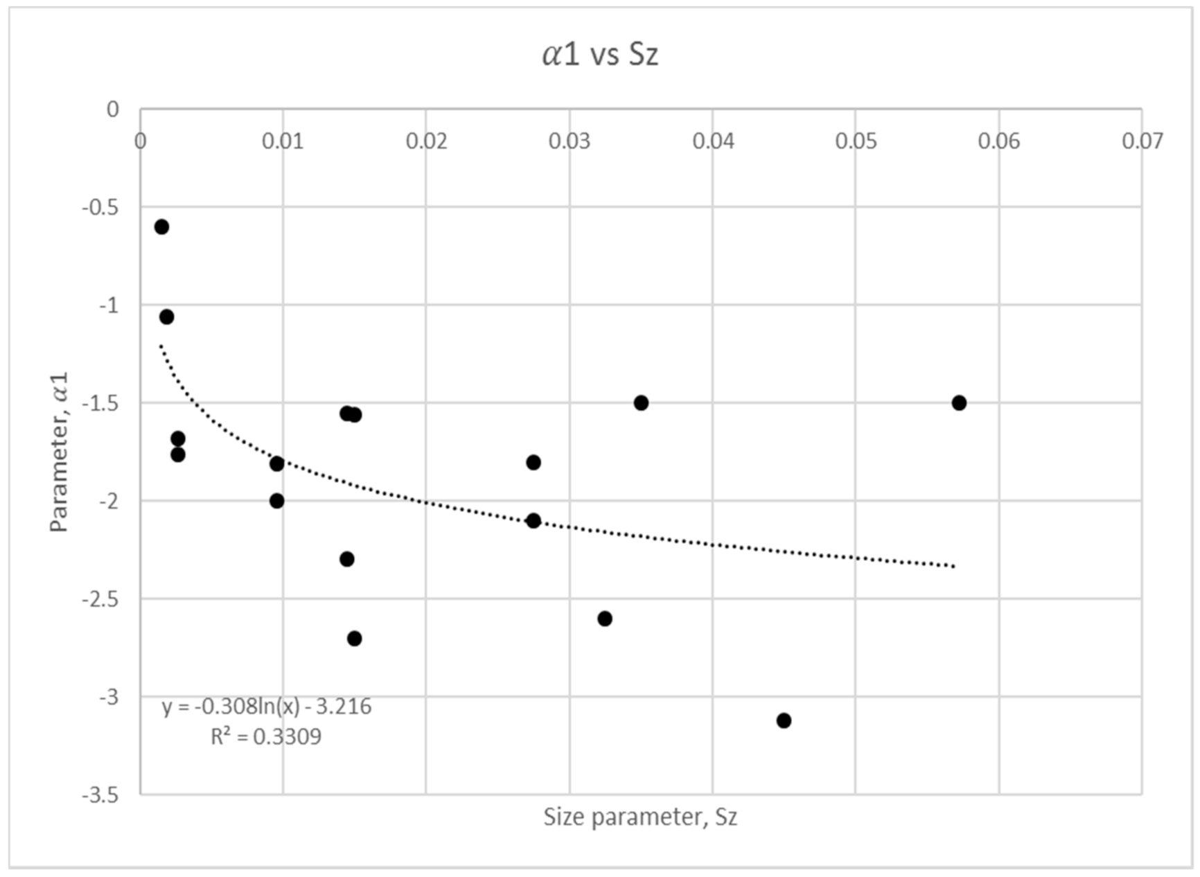
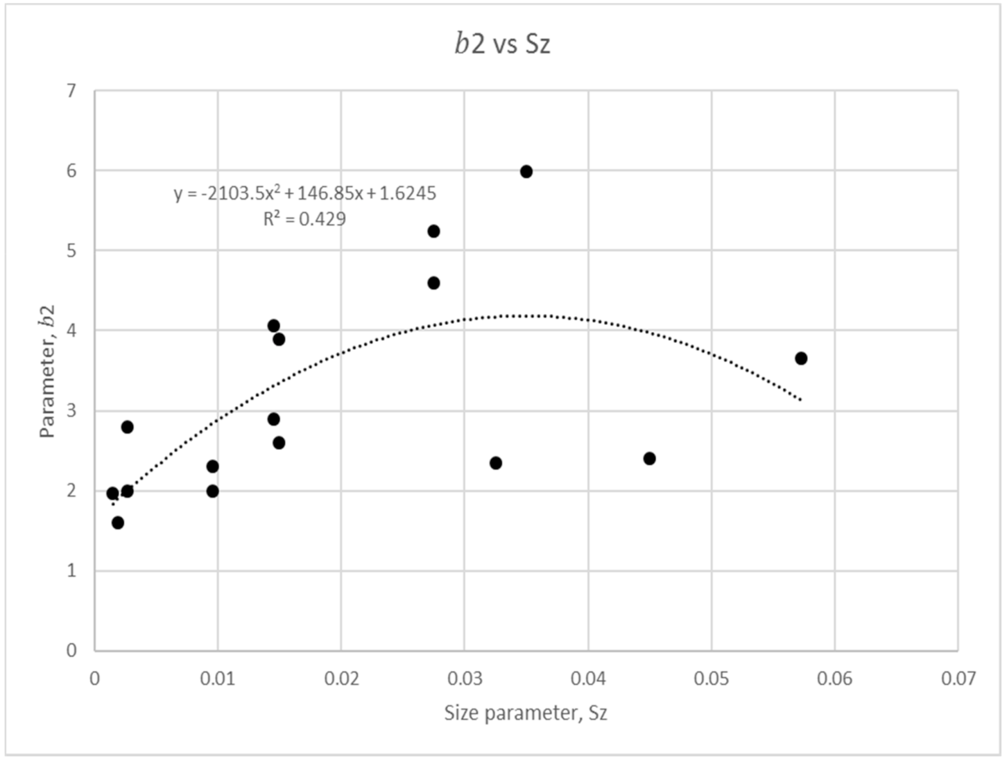
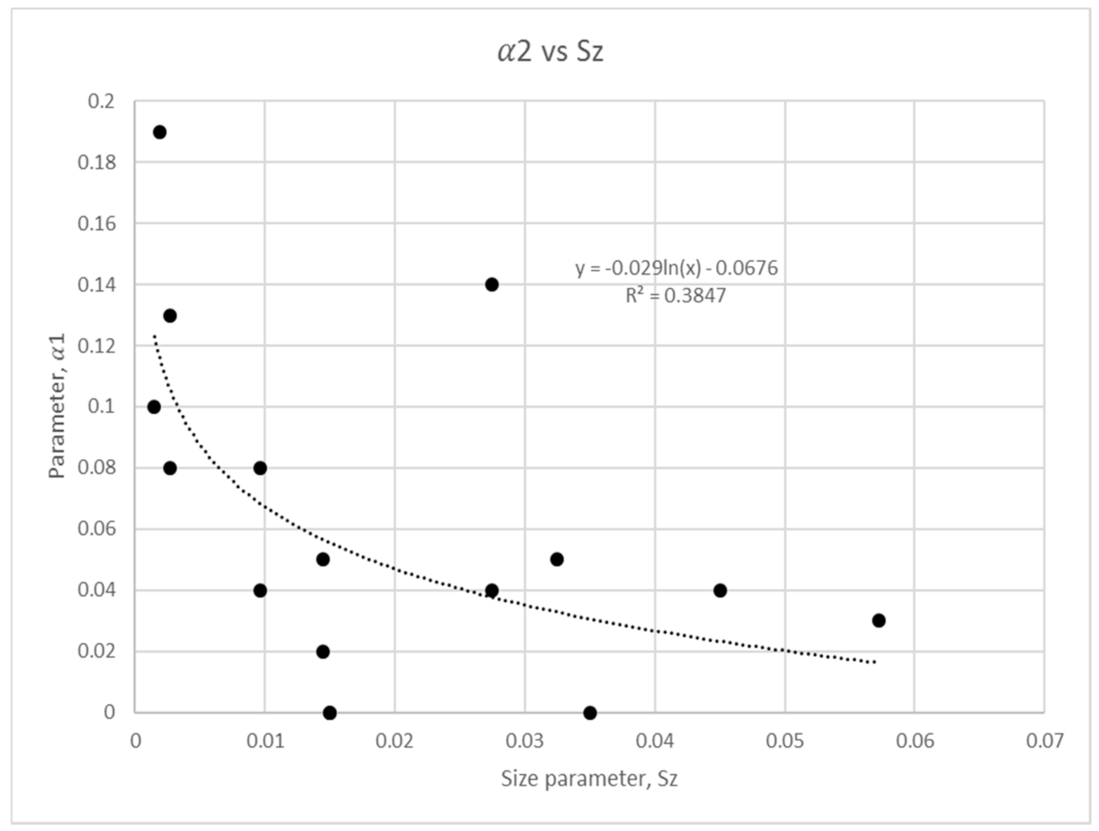
3.2. Size Parameter
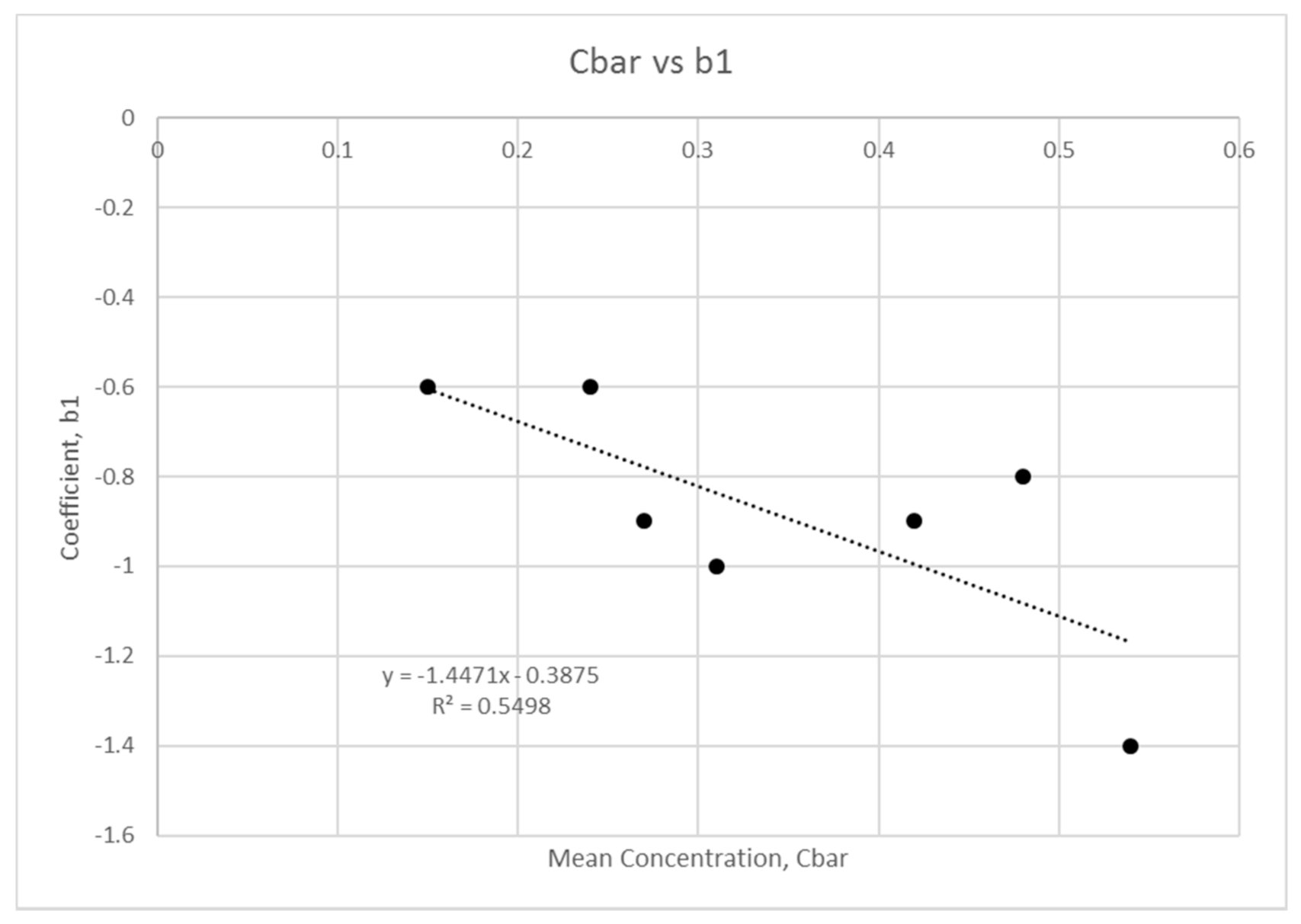
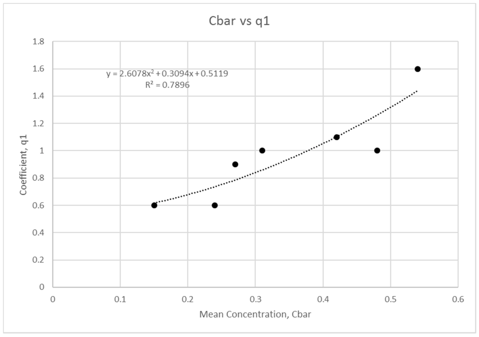
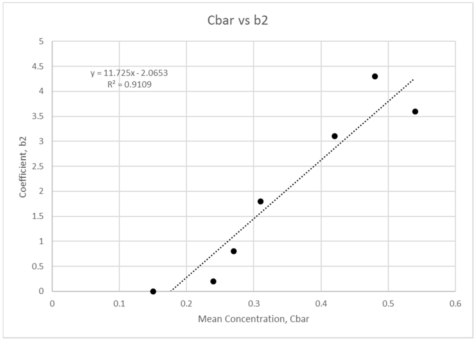
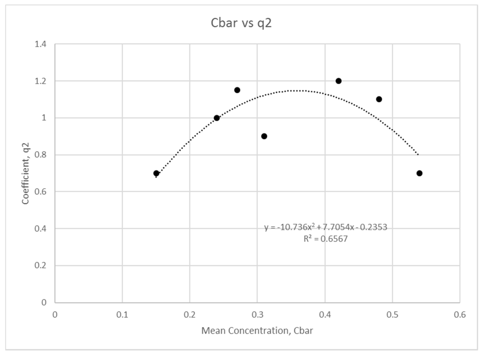
3.3. Mean Concentration
3.4. Hyper-To-Dilute Boundary
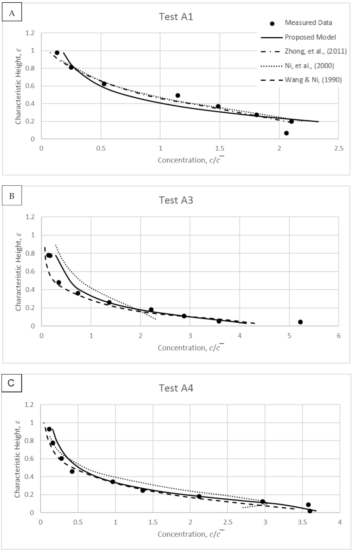
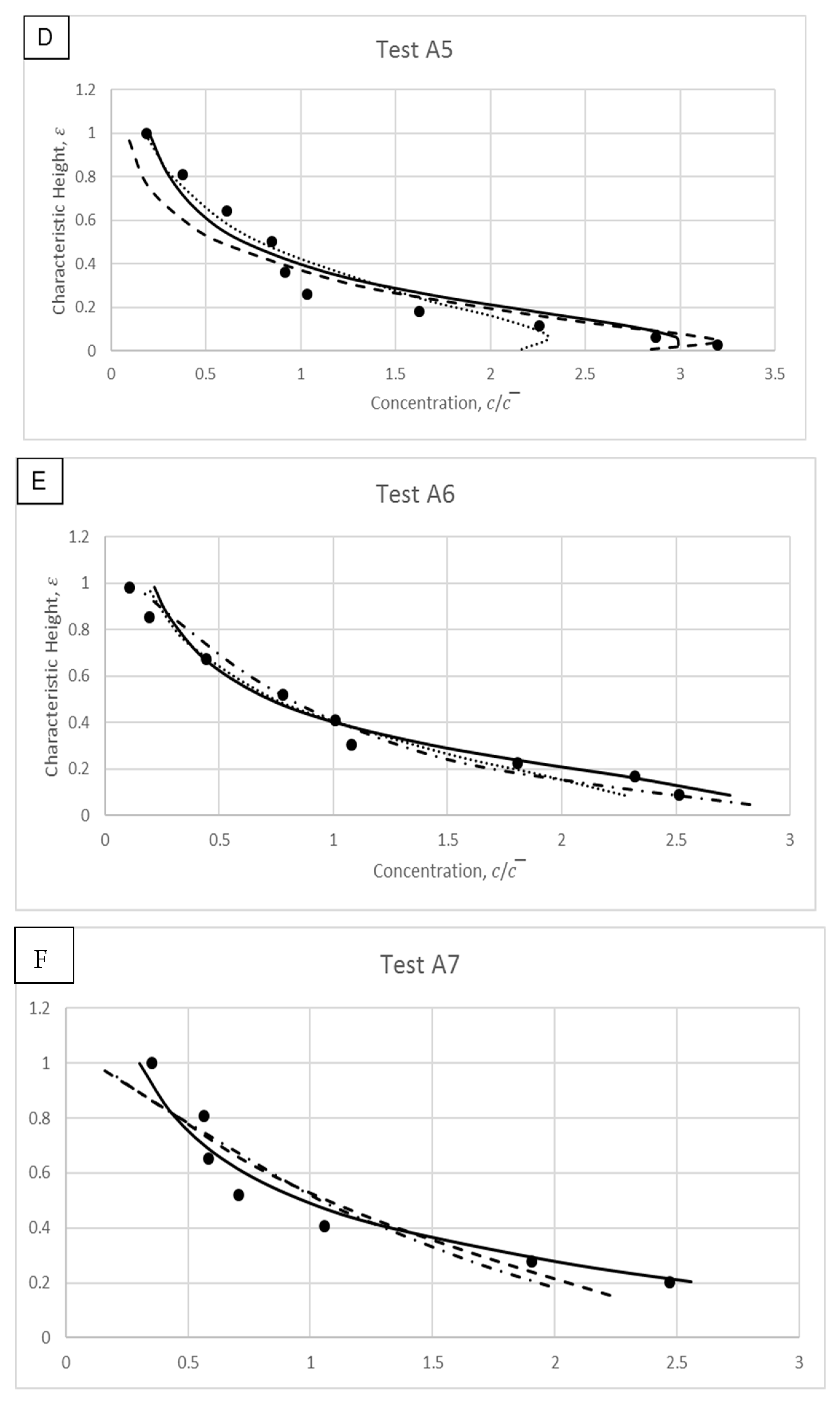
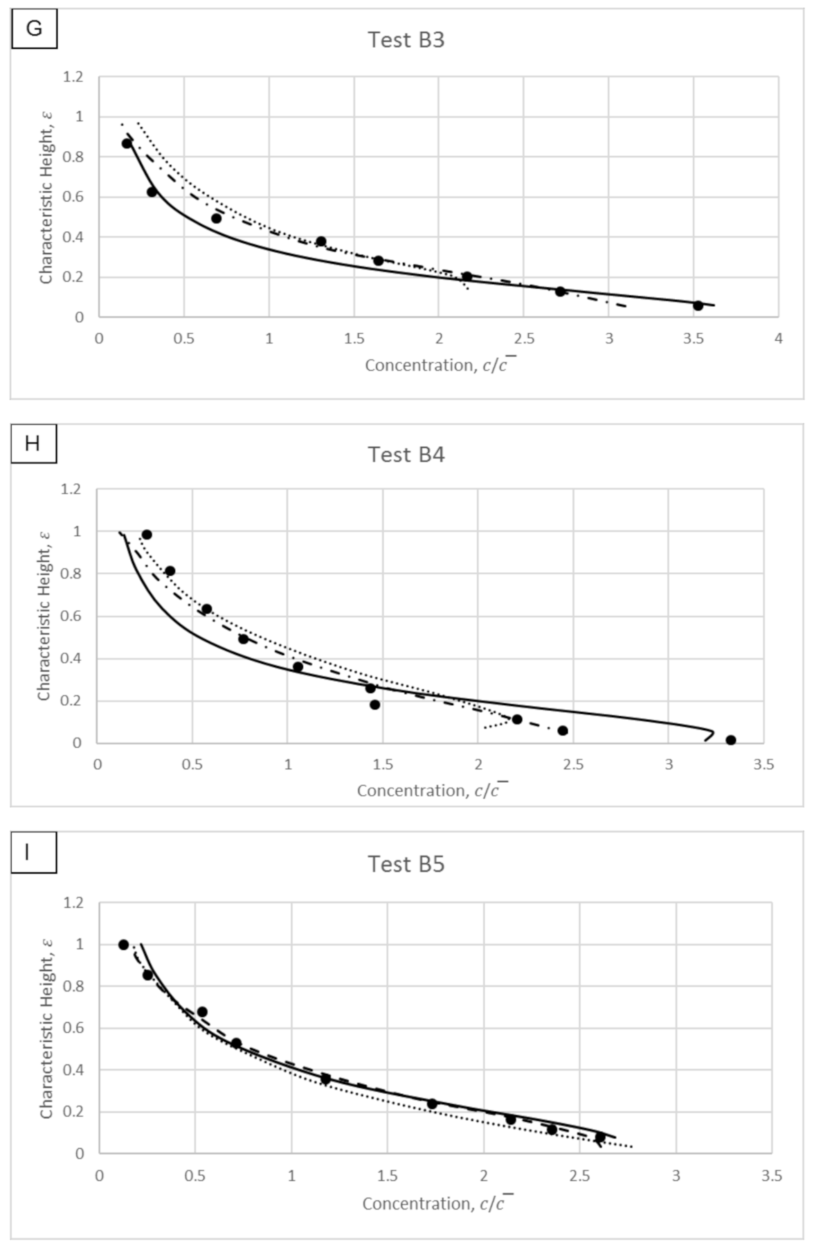
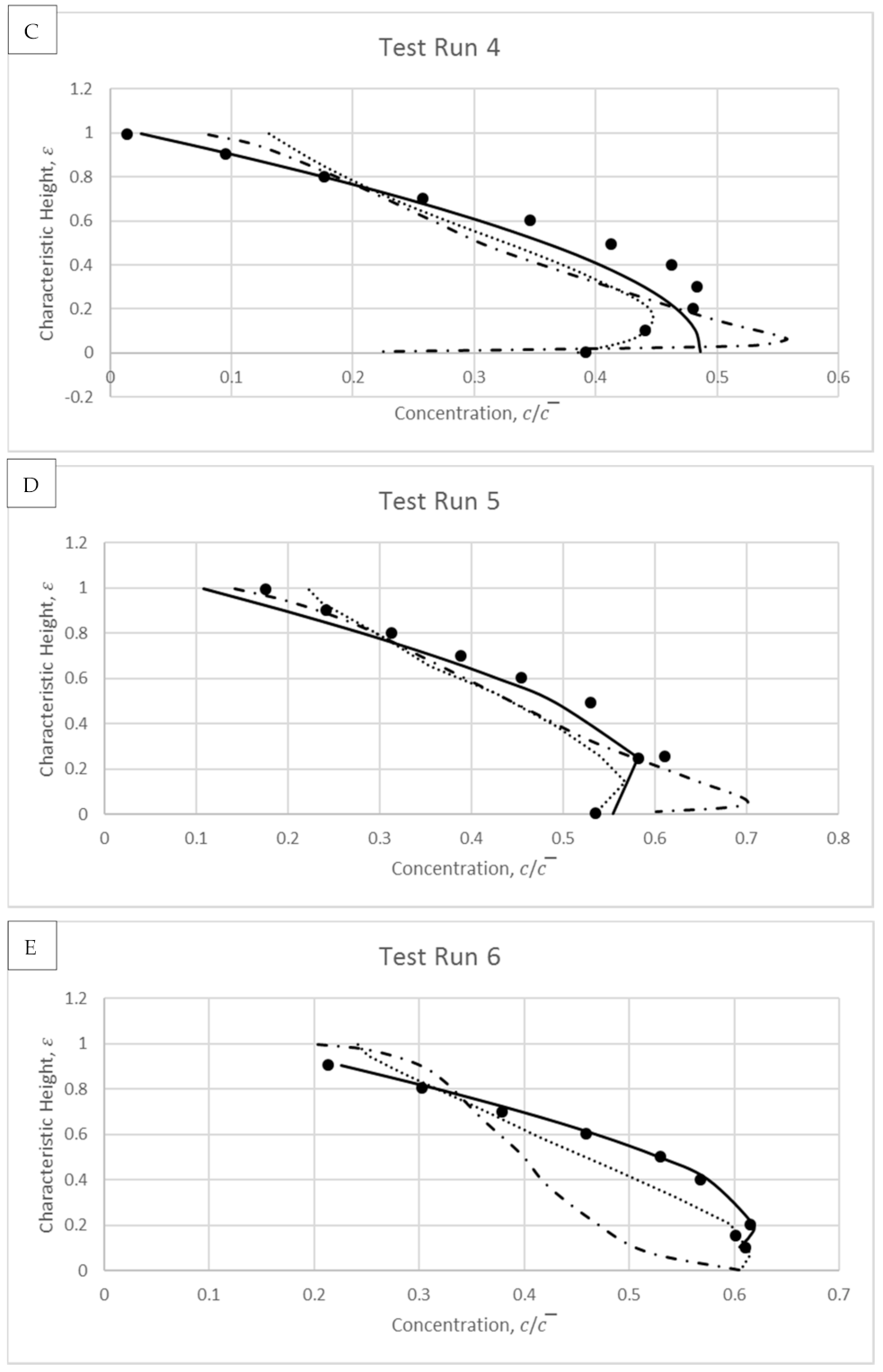
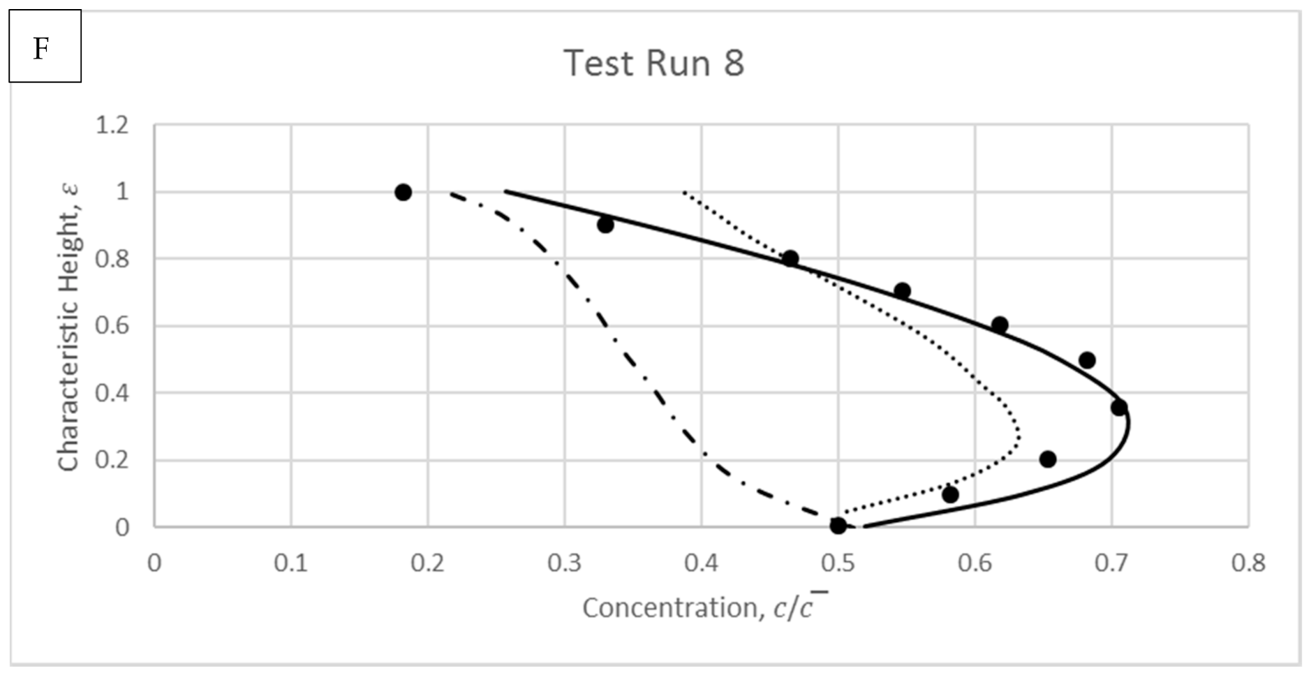
4. Model Validations
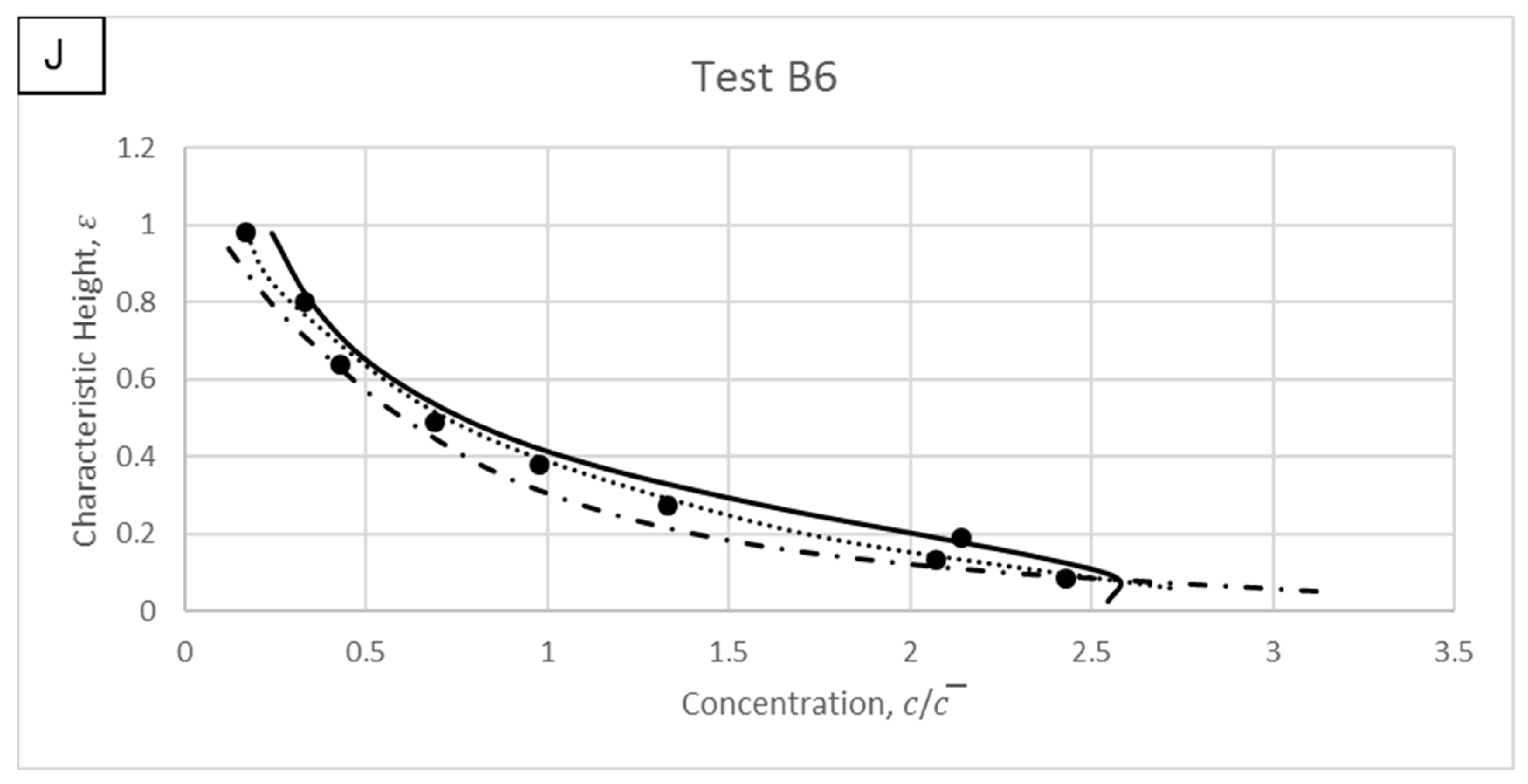
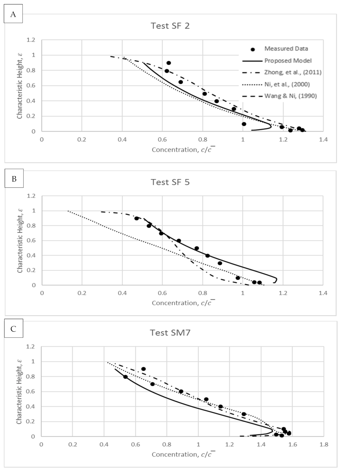
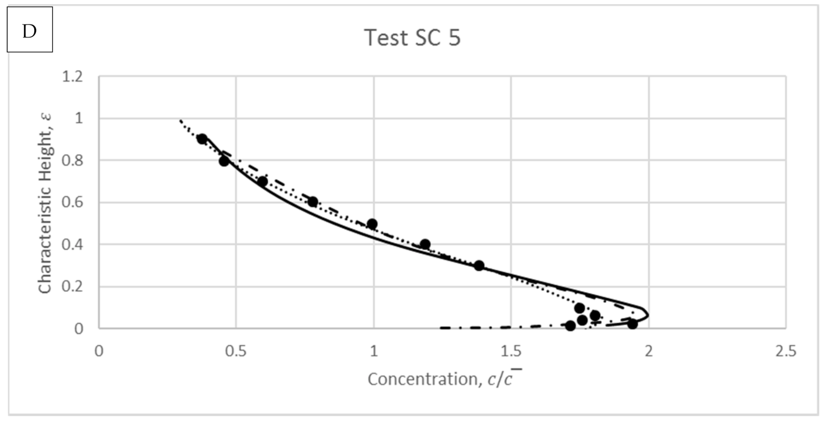
4.1. Wang and Ni
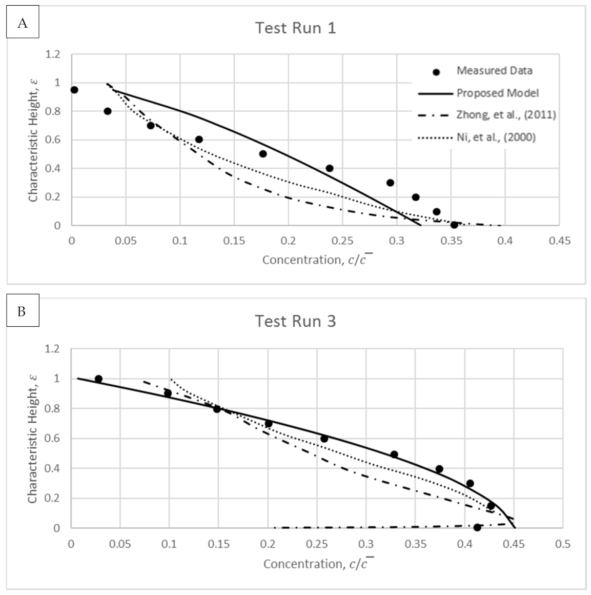
4.2. Wang and Qian
4.3. Michalik
5. Conclusions
Author Contributions
Funding
Institutional Review Board Statement
Informed Consent Statement
Data Availability Statement
Conflicts of Interest
References
- Pu, J.H.; Hussain, K.; Shao, S.-D.; Huang, Y.-F. Shallow sediment transport flow computation using time-varying sediment adaptation length. Int. J. Sediment Res. 2014, 29, 171–183. [Google Scholar] [CrossRef] [Green Version]
- Pu, J.H.; Wei, J.; Huang, Y. Velocity Distribution and 3D Turbulence Characteristic Analysis for Flow over Water-Worked Rough Bed. Water 2017, 9, 668. [Google Scholar] [CrossRef] [Green Version]
- Pu, J.H.; Huang, Y.; Shao, S.; Hussain, K. Three-Gorges Dam Fine Sediment Pollutant Transport: Turbulence SPH Model Simulation of Multi-Fluid Flows. J. Appl. Fluid Mech. 2016, 9, 1–10. [Google Scholar] [CrossRef]
- Pu, J.H. Turbulent rectangular compound open channel flow study using multi-zonal approach. Environ. Fluid Mech. 2018, 19, 785–800. [Google Scholar] [CrossRef] [Green Version]
- Pu, J.H.; Pandey, M.; Hanmaiahgari, P.R. Analytical modelling of sidewall turbulence effect on streamwise velocity profile using 2D approach: A comparison of rectangular and trapezoidal open channel flows. HydroResearch 2020, 32, 17–25. [Google Scholar] [CrossRef]
- Rouse, H. Modern Conceptions of the Mechanics of Fluid Turbulence. J. Pap. Trans. Am. Soc. Civ. Eng. 1937, 102, 463–505. [Google Scholar]
- Hsu, T.-J.; Jenkins, J.T.; Liu, P.L. On two-phase sediment transport: Dilute flow. J. Geophys. Res. Space Phys. 2003, 108, 3057. [Google Scholar] [CrossRef]
- Huang, S.-H.; Sun, Z.-L.; Xu, D.; Xia, S.-S. Vertical distribution of sediment concentration. J. Zhejiang Univ. A 2008, 9, 1560–1566. [Google Scholar] [CrossRef]
- Greimann, B.; Holly, F.M., Jr. Two-Phase Flow Analysis of Concentration Profiles. J. Hydraul. Eng. 2001, 127, 753–762. [Google Scholar] [CrossRef]
- Jha, S.K.; Bombardelli, F.A. Two-phase modeling of turbulence in dilute sediment-laden, open-channel flows. Environ. Fluid Mech. 2009, 9, 237–266. [Google Scholar] [CrossRef] [Green Version]
- Kundu, S.; Ghoshal, K. A mathematical model for type II profile of concentration distribution in turbulent flows. Environ. Fluid Mech. 2016, 17, 449–472. [Google Scholar] [CrossRef]
- Pu, J.H.; Lim, S.Y. Efficient numerical computation and experimental study of temporally long equilibrium scour development around abutment. Environ. Fluid Mech. 2013, 14, 69–86. [Google Scholar] [CrossRef] [Green Version]
- Liang, C.-F.; Abbasi, S.; Pourshahbaz, H.; Taghvaei, P.; Tfwala, S. Investigation of Flow, Erosion, and Sedimentation Pattern around Varied Groynes under Different Hydraulic and Geometric Conditions: A Numerical Study. Water 2019, 11, 235. [Google Scholar] [CrossRef] [Green Version]
- Kundu, S.; Ghoshal, K. Explicit formulation for suspended concentration distribution with near-bed particle deficiency. Powder Technol. 2014, 253, 429–437. [Google Scholar] [CrossRef]
- Wang, G.; Ni, J. The kinetic theory for dilute solid/liquid two-phase flow. Int. J. Multiph. Flow 1991, 17, 273–281. [Google Scholar] [CrossRef]
- Goeree, J.C.; Keetels, G.H.; Munts, E.A.; Bugdayci, H.H.; Van Rhee, C. Concentration and velocity profiles of sediment-water mixtures using the drift flux model. Can. J. Chem. Eng. 2016, 94, 1048–1058. [Google Scholar] [CrossRef]
- Pourshahbaz, H.; Abbasi, S.; Taghvaei, P. Numerical scour modeling around parallel spur dikes in FLOW-3D. J. Drink. Water Eng. Sci. 2017, 1–16. [Google Scholar] [CrossRef] [Green Version]
- Pourshahbaz, H.; Abbasi, S.; Pandey, M.; Pu, J.H.; Taghvaei, P.; Tofangdar, N. Morphology and hydrodynamics numerical simulation around groynes. ISH J. Hydraul. Eng. 2020, 1–9. [Google Scholar] [CrossRef]
- Ni, J.R.; Wang, G.Q.; Borthwick, A.G.L. Kinetic Theory for Particles in Dilute and Dense Solid-Liquid Flows. J. Hydraul. Eng. 2000, 126, 893–903. [Google Scholar] [CrossRef]
- Van Rijn, L.C. Sediment Transport, Part II: Suspended Load Transport. J. Hydraul. Eng. 1984, 110, 1613–1641. [Google Scholar] [CrossRef]
- McLean, S.R. On the calculation of suspended load for noncohesive sediments. J. Geophys. Res. Space Phys. 1992, 97, 5759. [Google Scholar] [CrossRef]
- Zhong, D.; Wang, G.; Sun, Q. Transport Equation for Suspended Sediment Based on Two-Fluid Model of Solid/Liquid Two-Phase Flows. J. Hydraul. Eng. 2011, 137, 530–542. [Google Scholar] [CrossRef]
- Fick, A. On liquid diffusion. J. Membr. Sci. 1995, 100, 33–38. [Google Scholar] [CrossRef]
- Almedeij, J. Asymptotic matching with a case study from hydraulic engineering. Proc. Recent Adv. Water Resour. Hydraul. Hydrol. Camb. 2009, 71–76. [Google Scholar] [CrossRef]
- Einstein, H.A.; Qian, N. Effects of Heavy Sediment Concentration Near the Bed on the Velocity and Sediment Distribution; Omaha: U.S. Army Engineer Division, Missouri River: Omaha, NE, USA, 1955. [Google Scholar]
- Bouvard, M.; Petković, S. Vertical dispersion of spherical, heavy particles in turbulent open channel flow. J. Hydraul. Res. 1985, 23, 5–20. [Google Scholar] [CrossRef]
- Sumer, B.; Kozakiewicz, A.; Fredsoe, J.; Deigaard, R. Velocity and Concentration Profiles in Sheet-Flow Layer of Movable Bed. J. Hydraul. Eng. 1996, 122, 549–558. [Google Scholar] [CrossRef]
- Kironoto, B.A.; Yulistiyanto, B. The validity of Rouse equation for predicting suspended sediment concentration profiles in transverse direction of uniform open channel flow. In Proceedings of the International Conference on Sustainable Development Water Waste Water Treatment, Yogyakarta, Indonesia, 14–15 December 2009. [Google Scholar]
- Kumbhakar, M.; Ghoshal, K.; Singh, V.P. Derivation of Rouse equation for sediment concentration using Shannon entropy. Phys. A Stat. Mech. Its Appl. 2017, 465, 494–499. [Google Scholar] [CrossRef]
- Coleman, N.L. Effects of Suspended Sediment on the Open-Channel Velocity Distribution. Water Resour. Res. 1986, 22, 1377–1384. [Google Scholar] [CrossRef]
- Wang, G.; Ni, J. Kinetic Theory for Particle Concentration Distribution in Two-Phase Flow. J. Eng. Mech. 1990, 116, 2738–2748. [Google Scholar] [CrossRef] [Green Version]
- Cellino, M.; Graf, W.H. Sediment-Laden Flow in Open-Channels under Noncapacity and Capacity Conditions. J. Hydraul. Eng. 1999, 125, 455–462. [Google Scholar] [CrossRef]
- Muste, M.; Yu, K.; Fujita, I.; Ettema, R. Two-phase versus mixed-flow perspective on suspended sediment transport in turbulent channel flows. Water Resour. Res. 2005, 41, 41. [Google Scholar] [CrossRef]
- Cheng, N.-S. Comparison of formulas for drag coefficient and settling velocity of spherical particles. Powder Technol. 2009, 189, 395–398. [Google Scholar] [CrossRef]
- Michalik, M.A. Density patterns of the inhomogeneous liquids in the industrial pipe-lines measured by means of radiometric scanning. La Houille Blanche 1973, 53–57. [Google Scholar] [CrossRef] [Green Version]
- Wang, X.; Qian, N. Turbulence Characteristics of Sediment-Laden Flow. J. Hydraul. Eng. 1989, 115, 781–800. [Google Scholar] [CrossRef]
- Ali, S.Z.; Dey, S. Mechanics of advection of suspended particles in turbulent flow. Proc. R. Soc. A Math. Phys. Eng. Sci. 2016, 472, 20160749. [Google Scholar] [CrossRef] [Green Version]


| Data Sources | |||||
|---|---|---|---|---|---|
| Bouvard and Petkovic [26] | 7.5 | 2.00–9.00 | 1.81–2.70 | 2.54–5.41 | 2.1–4.5 |
| Cellino and Graf [32] | 12.0 | 0.135 | 1.20 | 4.30–4.50 | 96–147 |
| Coleman [30] | 17.0–17.4 | 0.21–0.42 | 1.23–1.31 | 4.10 | 0.13-0.28 |
| Muste et al. [33] | 2.1 | 0.21–0.25 | 0.06 | 4.00–4.30 | 0.46–1.62 |
| Test No. | ||||
|---|---|---|---|---|
| A1 | 1.80 | 2.56 | 3.28 | 3.30 |
| A3 | 1.40 | 6.90 | 4.76 | 3.10 |
| A4 | 1.10 | 5.15 | 4.52 | 2.40 |
| A5 | 0.58 | 4.51 | 4.79 | 0.97 |
| A6 | 0.60 | 3.79 | 4.90 | 0.57 |
| A7 | 2.29 | 6.15 | 4.83 | 0.44 |
| B3 | 1.40 | 6.90 | 6.11 | 1.98 |
| B4 | 1.10 | 5.15 | 6.15 | 2.00 |
| B5 | 0.58 | 4.51 | 6.33 | 1.94 |
| B6 | 0.60 | 3.79 | 6.23 | 0.42 |
| Test No. | ||||
|---|---|---|---|---|
| SF2 | 0.268 | 0.197 | 7.74 | 10.2 |
| SF5 | 0.268 | 0.197 | 7.16 | 90.6 |
| SM7 | 0.960 | 1.590 | 7.37 | 75.4 |
| SC5 | 1.420 | 2.290 | 7.37 | 65.1 |
| Test No. | ||||
|---|---|---|---|---|
| Run 1 | 0.45 | 6.15 | 15.56 | 150 |
| Run 3 | 0.45 | 6.15 | 15.56 | 270 |
| Run 4 | 0.45 | 6.15 | 15.56 | 310 |
| Run 5 | 0.45 | 6.15 | 15.56 | 420 |
| Run 6 | 0.45 | 6.15 | 15.56 | 450 |
| Run 8 | 0.45 | 6.15 | 15.56 | 540 |
Publisher’s Note: MDPI stays neutral with regard to jurisdictional claims in published maps and institutional affiliations. |
© 2021 by the authors. Licensee MDPI, Basel, Switzerland. This article is an open access article distributed under the terms and conditions of the Creative Commons Attribution (CC BY) license (http://creativecommons.org/licenses/by/4.0/).
Share and Cite
Pu, J.H.; Wallwork, J.T.; Khan, M.A.; Pandey, M.; Pourshahbaz, H.; Satyanaga, A.; Hanmaiahgari, P.R.; Gough, T. Flood Suspended Sediment Transport: Combined Modelling from Dilute to Hyper-Concentrated Flow. Water 2021, 13, 379. https://doi.org/10.3390/w13030379
Pu JH, Wallwork JT, Khan MA, Pandey M, Pourshahbaz H, Satyanaga A, Hanmaiahgari PR, Gough T. Flood Suspended Sediment Transport: Combined Modelling from Dilute to Hyper-Concentrated Flow. Water. 2021; 13(3):379. https://doi.org/10.3390/w13030379
Chicago/Turabian StylePu, Jaan H., Joseph T. Wallwork, Md. Amir Khan, Manish Pandey, Hanif Pourshahbaz, Alfrendo Satyanaga, Prashanth R. Hanmaiahgari, and Tim Gough. 2021. "Flood Suspended Sediment Transport: Combined Modelling from Dilute to Hyper-Concentrated Flow" Water 13, no. 3: 379. https://doi.org/10.3390/w13030379