
Evaluation of Rainfall Erosivity Factor Estimation Using Machine and Deep Learning Models
by
 , , and
Jimin Lee
1, 
Seoro Lee
1,
Jiyeong Hong
1 ,
,
Dongjun Lee
1,
Joo Hyun Bae
2,
Jae E. Yang
3,
Jonggun Kim
1 and
Kyoung Jae Lim
1,* 1
Department of Regional Infrastructure Engineering, Kangwon National University, Chuncheon-si 24341, Korea
2
Korea Water Environment Research Institute, Chuncheon-si 24408, Korea
3
Department of Biological Environment, Kangwon National University, Chuncheon-si 24341, Korea
*
Author to whom correspondence should be addressed.
Water 2021, 13(3), 382; https://doi.org/10.3390/w13030382
Submission received: 17 December 2020
/
Revised: 27 January 2021
/
Accepted: 28 January 2021
/
Published: 1 February 2021
(This article belongs to the Special Issue Soil–Water Conservation, Erosion, and Landslide)
Abstract
:Rainfall erosivity factor (R-factor) is one of the Universal Soil Loss Equation (USLE) input parameters that account for impacts of rainfall intensity in estimating soil loss. Although many studies have calculated the R-factor using various empirical methods or the USLE method, these methods are time-consuming and require specialized knowledge for the user. The purpose of this study is to develop machine learning models to predict the R-factor faster and more accurately than the previous methods. For this, this study calculated R-factor using 1-min interval rainfall data for improved accuracy of the target value. First, the monthly R-factors were calculated using the USLE calculation method to identify the characteristics of monthly rainfall-runoff induced erosion. In turn, machine learning models were developed to predict the R-factor using the monthly R-factors calculated at 50 sites in Korea as target values. The machine learning algorithms used for this study were Decision Tree, K-Nearest Neighbors, Multilayer Perceptron, Random Forest, Gradient Boosting, eXtreme Gradient Boost, and Deep Neural Network. As a result of the validation with 20% randomly selected data, the Deep Neural Network (DNN), among seven models, showed the greatest prediction accuracy results. The DNN developed in this study was tested for six sites in Korea to demonstrate trained model performance with Nash–Sutcliffe Efficiency (NSE) and the coefficient of determination (R2) of 0.87. This means that our findings show that DNN can be efficiently used to estimate monthly R-factor at the desired site with much less effort and time with total monthly precipitation, maximum daily precipitation, and maximum hourly precipitation data. It will be used not only to calculate soil erosion risk but also to establish soil conservation plans and identify areas at risk of soil disasters by calculating rainfall erosivity factors.
1. Introduction
Climate change and global warming have been concerns for hydrologists and environmentalists [1,2,3]. Hydrologic change is expected to be more aggressive as a result of rising global temperature, that consequently results in a change in the current rainfall patterns [4]. Moreover, the Intergovernmental Panel on Climate Change (IPCC) [5] report showed that increasing rainfall events and rainfall intensity are expected to occur in the coming years [6]. Due to the frequent occurrence of greater intensity rainfall events, rainfall erosivity will increase, thus topsoil will become more vulnerable to soil erosion [7]. Soil erosion by extreme intensive rainfall is a significant issue from agricultural and environmental perspectives [8]. A decrease in soil fertility, the inflow of sediment into the river ecosystem, reduction of crop yields, etc., will occur due to soil erosion [9,10]. Therefore, effective best management practices should be implemented for better sustainable management of soil erosion. Furthermore, there is a need for a regional estimate of soil loss to proper decision-making related to appropriate control practice, since erosion occurs diversely over space and time [11].
During the last few decades, various empirical, physically based, and conceptual computer models [12] such as Soil and Water Assessment Tool (SWAT) [13], European Soil Erosion Model (EUROSEM) [14], Water Erosion Prediction Project (WEPP) [15], Sediment Assessment Tool for Effective Erosion Control (SATEEC) [16], Agricultural Non-Point Source Pollution Model (AGNPS) [17], Universal Soil Loss Equation (USLE) [18], Revised Universal Soil Loss Equation (RUSLE) [19] have been developed. Among the models, the USLE model is one of the most popular and widely used empirical erosion models to predict soil erosion because of its easy application and simple structures [20,21]. The USLE model [18] calculates the annual average amount of soil erosion by taking into account soil erosion factors, such as rainfall erosivity factors, soil erodibility factor, slope and length, crop and cover management factor, and conservation practice factor.
The Ministry of Environment of Korea has supported for use of USLE in planning and managing sustainable land management in Korea. To these ends, the USLE has been extensively used to predict soil erosion and evaluate various soil erosion best management practices (BMPs) in Korea. Various efforts have been made for the development of site-specific USLE parameters over the years [22]. Yu et al. [23] suggested monthly soil loss prediction at Daecheong Dam basin in order to improve the limitation of annual soil loss prediction. They found that over 50% of the annual soil loss occurs during July and August. The rainfall erosivity factor (R-factor) is one of the factors to be parameterized in the evaluation of soil loss in the USLE. The R-factor values are affected by the distribution of rainfall amount and its intensity over time and space.
Rainfall erosivity has been widely investigated due to its impact on soil erosion studies worldwide. Rainfall data at intervals of less than 30 min are required to calculate USLE rainfall erosivity factors. The empirical equations related to R-factor based on rainfall data, such as daily, monthly, or yearly, available in various spatial and temporal extents, have been developed using numerous data [24,25].
Sholagberu et al. [26] proposed a regression equation based on annual precipitation because it is difficult to collect sub-hourly rainfall data to calculate maximum 30-min rainfall intensity. Risal et al. [27] proposed a regression equation that can calculate monthly rainfall erosivity factors from 10-min interval rainfall data. In addition, the Web ERosivity Module (WERM), web-based software that can calculate rainfall erosivity factor, was developed and made available at http://www.envsys.co.kr/~werm. In the study by Risal et al. [27] on the R-factor calculation for South Korea, 10-min interval rainfall data, which cannot give the exact estimate of maximum 30-min rainfall intensity, was used. The Korea Meteorological Administration (KMA) provides 1-min rainfall data for over 50 weather stations in Korea. Estimation of R-factor values for South Korea using a recent rainfall dataset is needed for present and future uses because climate change causes changes in precipitation pattern and intensity to some degrees. However, the process of calculation of R-factor from rainfall data is time-consuming, although the Web ERosivity Module (WERM) software can calculate rainfall erosivity factor [27]. Furthermore, the radar rainfall dataset can be used to calculate spatial USLE R raster values using Web Erosivity Model-Spatial (WERM-S) [28]. These days, Machine Learning/Deep Learning (ML/DL) has been suggested as an alternative to predict and simulate natural phenomena [29]. Thus, ML/DL has been used for the prediction of flow, water quality, and ecosystem services [30,31,32,33,34]. These studies have implied that ML/DL is an efficient and effective way to calculate R factor values using recent rainfall time-series data provided by the KMA.
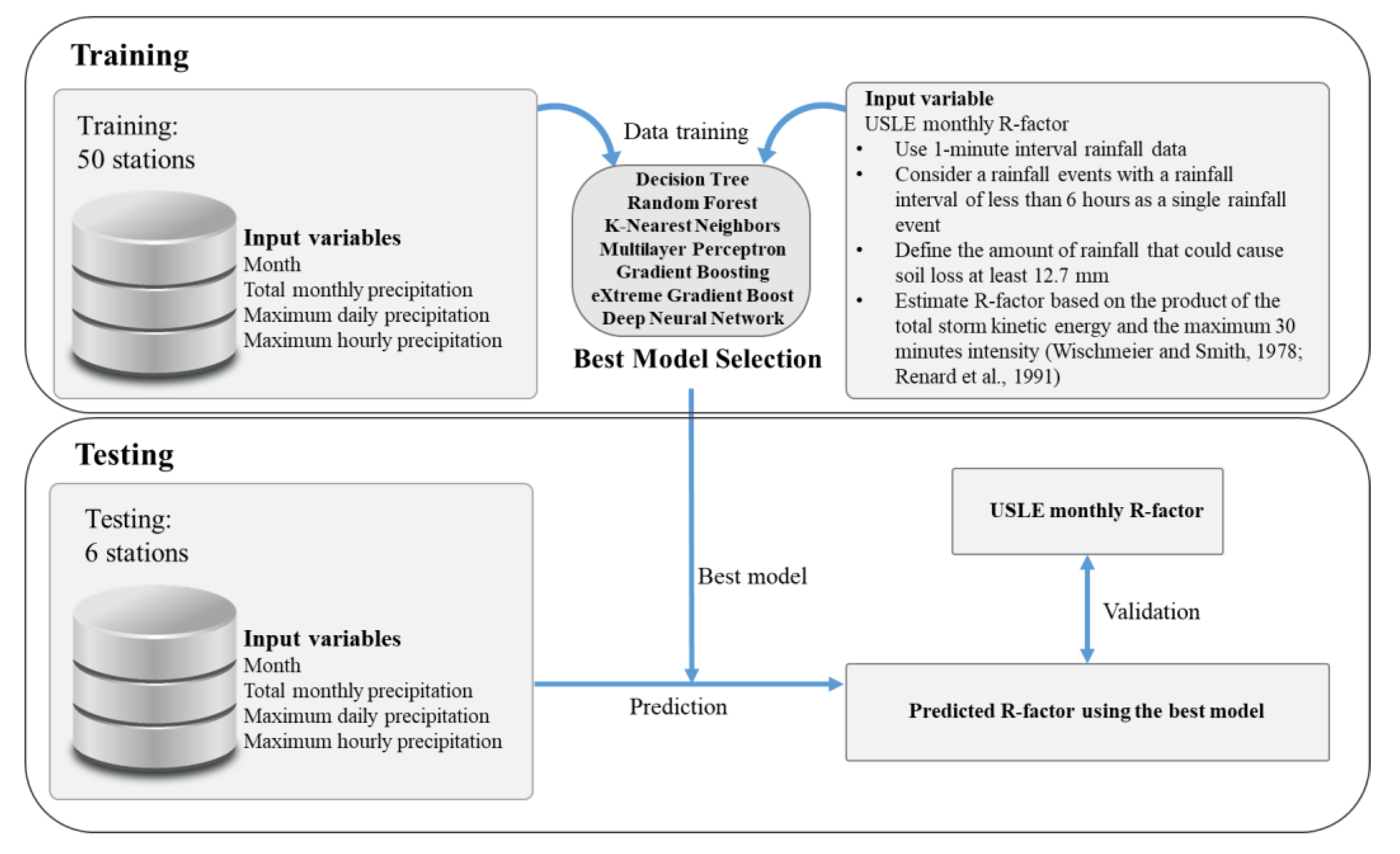
The objective of this study is to develop machine learning models to predict the monthly R-factor values, which are comparable with those calculated by the USLE method. For this aim, we calculated R-factor using 1-min interval rainfall data to estimate the maximum 30-min rainfall intensity of the target values, which is monthly R factor values at 50 stations in S. Korea. In the previous study by Risal et al. [27], the R-factor values for South Korea were calculated using 10-min interval rainfall data, which cannot give an exact estimate of maximum 30-min rainfall intensity. The procedure used in this study is shown in Figure 1.
2. Methods
2.1. Study Area
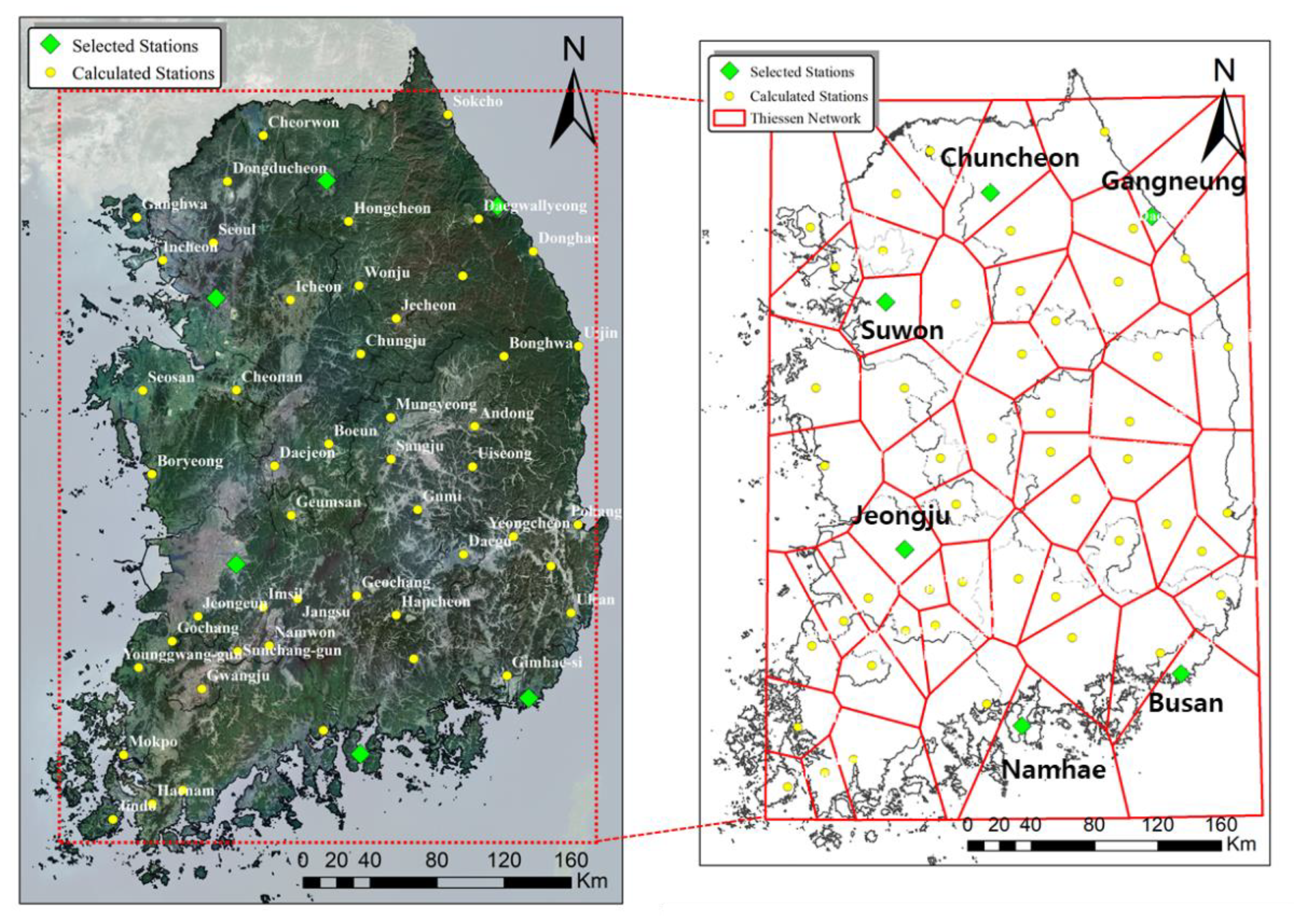
Figure 2 shows the location of weather stations where 1-min rainfall data have been observed over the years in South Korea. The fifty points marked in circles are observational stations that provide data used for training and validation to create machine learning models predicting rainfall erosivity factors, while six stations marked in green on the right map—Chuncheon, Gangneung, Suwon, Jeonju, Busan, and Namhae—represent the stations for the final evaluation of the results predicted by machine learning models selected through validation. Thiessen network presented using red lines of the map on the right shows a range of the weather environment around the weather stations.
2.2. Monthly Rainfall Erosivity Calculation
Monthly rainfall erosivity (R-factor) was calculated for each of the 50 weather stations in South Korea from 2013 to 2019. It was calculated based on the equation given in the USLE users’ manual in order to calculate the R-factor value [18]. According to Wischmeier and Smith [18], a rainfall interval of fewer than six hours is considered a single rainfall event. In addition, the least amount of rainfall that could cause soil loss is at least 12.7 mm or more as specified in the USLE users’ manual [35].
However, if the rainfall is 6.25 mm during 15 min, it is defined as a rainfall event that can cause soil loss. The calculations for each rainfall event are as follows.
where I (mm h−1) is the intensity of rainfall, e (MJ mm ha−1) is unit rainfall energy, P (mm) is the rainfall volume during a given time period, E (MJ ha−1) is the total storm kinetic energy, I30max (mm h−1) is the maximum 30-min intensity in the erosive event, and R (MJ mm ha−1 h−1) is the rainfall erosivity factor. In this study, the monthly R-factor (MJ mm ha−1 h−1 month−1) was estimated by calculating monthly E and multiplying it by I30max. In addition, the monthly rainfall erosivity factor was calculated using Equations (1)–(4) [18] using the 1-min precipitation data provided on the Meteorological Data Open Portal site of the KMA (Korea Meteorological Administration).
IF I ≤ 76 mm/hr → e = 0.119 + 0.0873log10 I
IF I > 76 mm/hr → e = 0.283
E = Σ (e × P)
R = E × I30max
2.3. Machine Learning Models
Machine learning can be largely divided into supervised learning, unsupervised learning, and reinforcement learning [36,37]. In this study, supervised learning algorithms were used. A total of seven methods (Table 1) were used to build models to estimate R-factor. Table 1 shows the information on machine learning models utilized in this study.
Decision Tree, Random Forest, K-Nearest Neighbors, Gradient Boosting, and Multilayer Perceptron imported and used the related functions from the Scikit-learn module (Version: 0.21.3), while eXtreme gradient boost was taken from the XGboost library (License: Apache-2.0) and used the regression functions. Deep Neural Network is trained by taking Dense and Dropout functions from “Keras.models.Sequential” module of TensorFlow (Version: 2.0.0) and Keras (Version: 2.3.1) framework. In this study, the standardization method was used during the pre-process for raw data. Moreover, the “StandardScaler” function, a preprocessing library of Scikit-learn, was used.
2.3.1. Decision Tree
The Decision Tree (DT) model uses hierarchical structures to find structural patterns in data for constructing decision-making rules to estimate both dependent and independent variables [38]. It first learns by continuing the yes/no question to reach a decision [39]. In this study, the DT model in the Scikit-learn supports only the pre-pruning. Entropy was based on classification and 2 for min_samples_split was given in Table 2.
A model hyperparameter is a value that is set directly by the user when modeling. Table 2 shows the hyperparameter settings of the regressors used in this study.
2.3.2. Random Forest
Random Forest (RF) is a decision tree algorithm developed by Breiman [40] that applies the Bagging algorithm among the Classification and Registration Tree (CART) algorithm and the ensemble technique. RF creates multiple training data from a single dataset and performs multiple training. It generates several decision trees and improves predictability by integrating the decision trees [41]. Detailed tuning of the hyperparameter in RF is easier than an artificial neural network and support vector regression [42].
In this study, the hyperparameters in the RF are the following: 52 for n_estimators, and 1 for min_samples_leaf.
2.3.3. K-Nearest Neighbors
K-Nearest Neighbors (KNN) is a non-parametric method which can be used for regression and classification [43]. In this study, KNN was used for regression. KNN is an algorithm that finds the nearest “K” neighborhood from the new data in training data and uses the most frequent class of these neighbors as a predicted value [44]. In this study, the number of the nearest neighbors in KNN’s hyperparameter was set as 3. The weights were calculated using a simple mean, and the distance was calculated by the Minkowski method [45].
2.3.4. Gradient Boosting and eXtreme Gradient Boost
Gradient Boosting (GB) is an ensemble algorithm belonging to the boosting family that can perform classification and regression analysis [46,47]. In GB, the gradient reveals the weaknesses of the model that have been learned so far, whereas other machine learning models (e.g., DT and RF) focus on it to boost performance [48]. In other words, the advantage of gradient boosting is that the other loss functions can be used as much as possible. Therefore, the parameters that minimize the loss function that quantifies errors in the predictive model can found for better R-factor prediction. In this study, the hyperparameters in the GB are the following: 0.01 for learning_rate, 4 for min_samples_split.
The eXtreme Gradient Boost (XGB) model is faster in training and classifying data than GB using parallel processing. It also has a regulatory function that prevents overfitting, which results in better predictive performance [49]. XGB is trained only by important features so that it calculates faster and performs better when compared to other algorithms [50,51]. The hyperparameters in the XGB are the following: gbtree for booster, and 10 for max_depth.
2.3.5. Multilayer Perceptron
Multilayer Perceptron (MLP) is a neural network that uses a back-propagation algorithm to learn weights [52]. MLP network consists of an input layer, a hidden layer, and an output layer (the R-factor). In this study, the hidden layer consisted of 50 nodes.
The hidden layers receive the signals from the nodes of the input layer and transform them into signals that are sent to all output nodes, transforming them into the last layer of outputs [53]. The output is used as input units in the subsequent layer. The connection between units in subsequent layers has a weight. MLP learns its weights by using the backpropagation algorithm [52].
2.3.6. Deep Neural Network
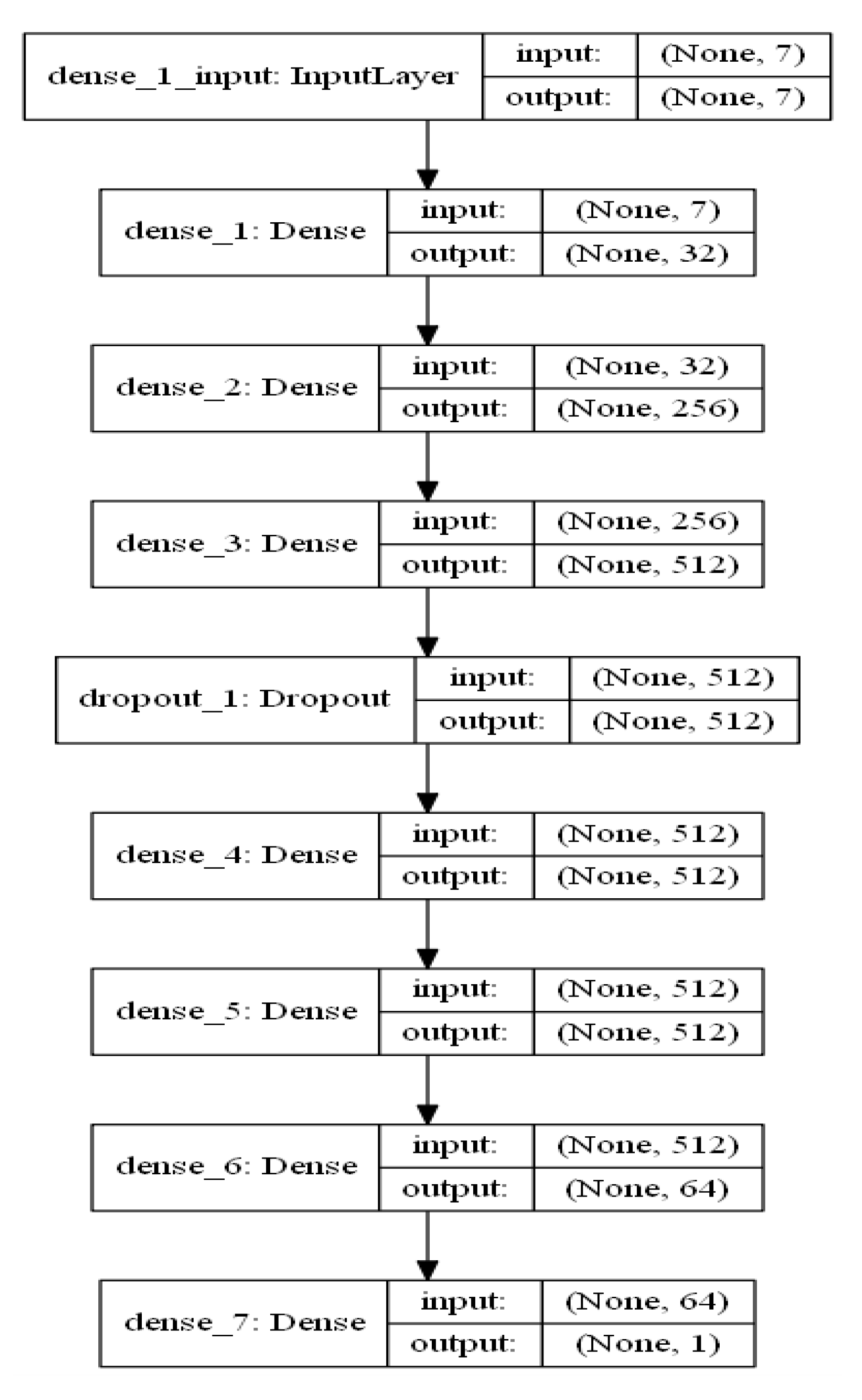
Deep Neural Network (DNN) is a predictive model that uses multiple layers of computational nodes for extracting features of existing data and depending on patterns learn to predict the outcome of some future input data [54]. The invention of the new optimizers enables us to train a large number of hyperparameters more quickly. In addition, the regularization and dropout allow us to avoid overfitting. The package used to build DNN in this study was TensorFlow developed by Google. In this study, the DNN model structure consisted of 7 dense layers and 1 dropout (Figure 3). Additional details about DNN can be found in Hinton et al. [55].
2.4. Input Data and Validation Method
Input data were compiled as shown in Table 3 to develop machine learning models to assess the R factor. The corresponding month from Jan. to Dec. was altered to numerical values, because rainfall patterns and their intensity may vary every month over space. Total monthly precipitation, maximum daily precipitation, and maximum hourly precipitation were calculated monthly and selected as the independent variables. The data can be easily downloaded in the form of monthly and hourly data among the Automated Synoptic Obstruction System (ASOS) data from the Korea Meteorological Administration (KMA)’s weather data opening portal site and organized as input data.
The monthly R-factors data in the manner presented in the USLE for the 50 selected sites from 2013 to 2019 were designated as target values, and as the features are given in Table 4, month (1–12), total monthly precipitation, maximum daily precipitation, and maximum hourly precipitation were designated as the features. Among the data, 80% of randomly selected data were trained, the model was created, and then the remaining 20% of data were used for the validation of the trained model.
To assess the performance of each machine learning model, Nash–Sutcliffe efficiency (NSE), Root Mean Squared Errors (RMSE), the Mean Absolute Error (MAE), and coefficient of determination (R2) was used. Numerous studies indicated the appropriateness of these measures to assess the accuracy of hydrological models [56,57,58]. NSE, RMSE, MAE, and R2 for evaluation of the model accuracy can be calculated from Equations (5)–(8).
where is the actual value of t, is the mean of the actual value, is the estimated value of t, is the mean of the estimated value, and n is the total number of data.
3. Results and Discussion
3.1. USLE R-Factor
For the selected 50 sites, monthly rainfall erosivity factors for each year from 2013 to 2019 were calculated, and the average monthly rainfall erosivity factors for seven years were obtained. Then, the seven-year average monthly rainfall erosivity, R-factor, was generated and shown in Table 1. Moreover, to give a comprehensive look at the degree of rainfall patterns by site, the average annual rainfall erosivity factor for each site is also presented in Table 4.
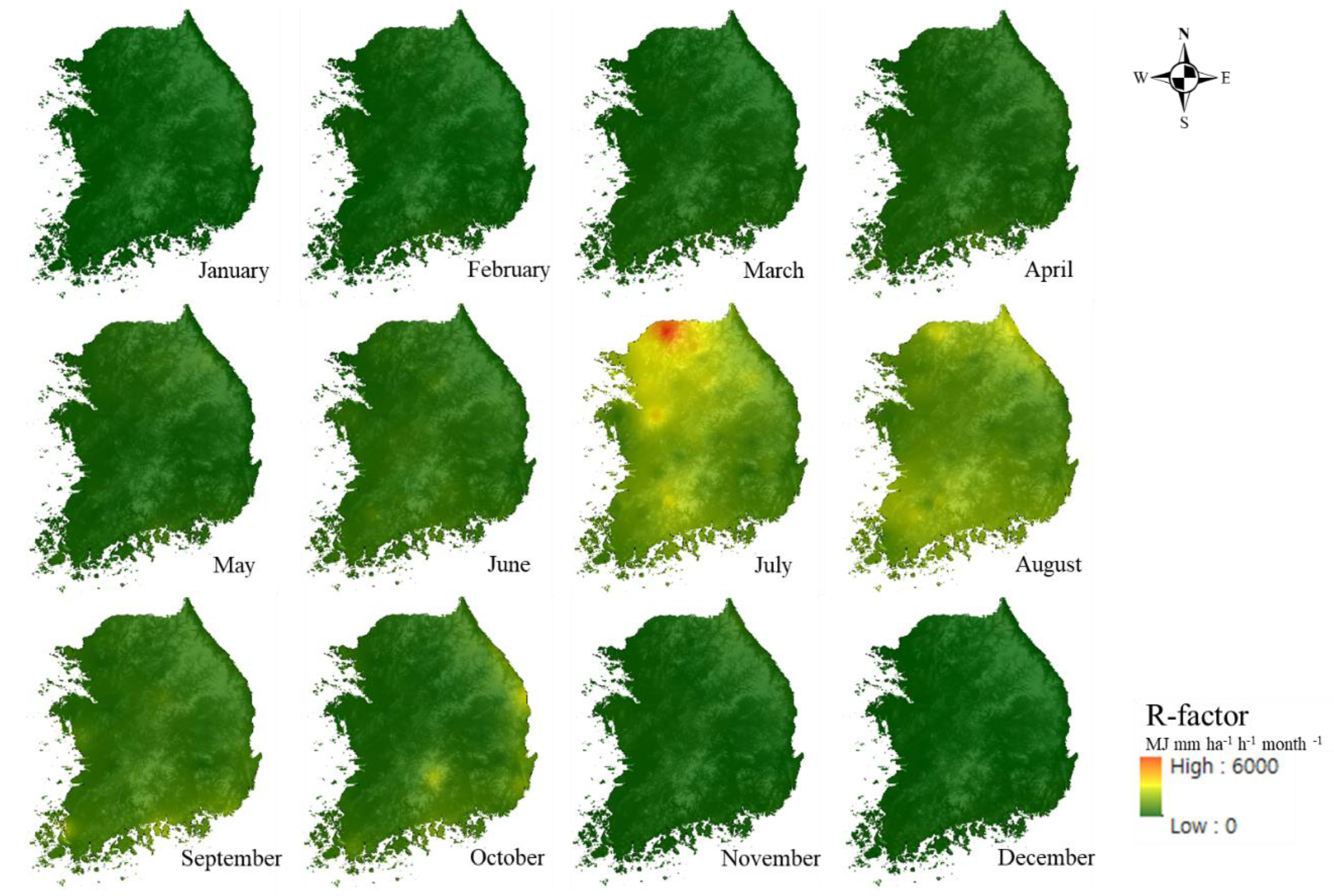
In this study, rainfall erosivity factor maps were generated to examine patterns of monthly R-factor calculated by USLE using rainfall data from 50 selected sites for evaluation. The R-factor distributions were mapped reflecting the geographical characteristics in South Korea (Figure 4). The high R-factor distribution in all regions during the summer months of July and August can be confirmed.
The monthly R-factors for two months from July to August contribute more than 50% of the total average annual R factor value of Korea. The rainfall occurs mainly in the wet season and the likelihood of erosion is very high compared to the dry season. In such a case, using the average annual R-factor value can give a misleading amount of soil erosion. For these reasons, the monthly R-factor would be helpful in analyzing the impact of the rainfall on soil erosion rather than the average annual R-factor.
3.2. Validation of Machine Learning Models
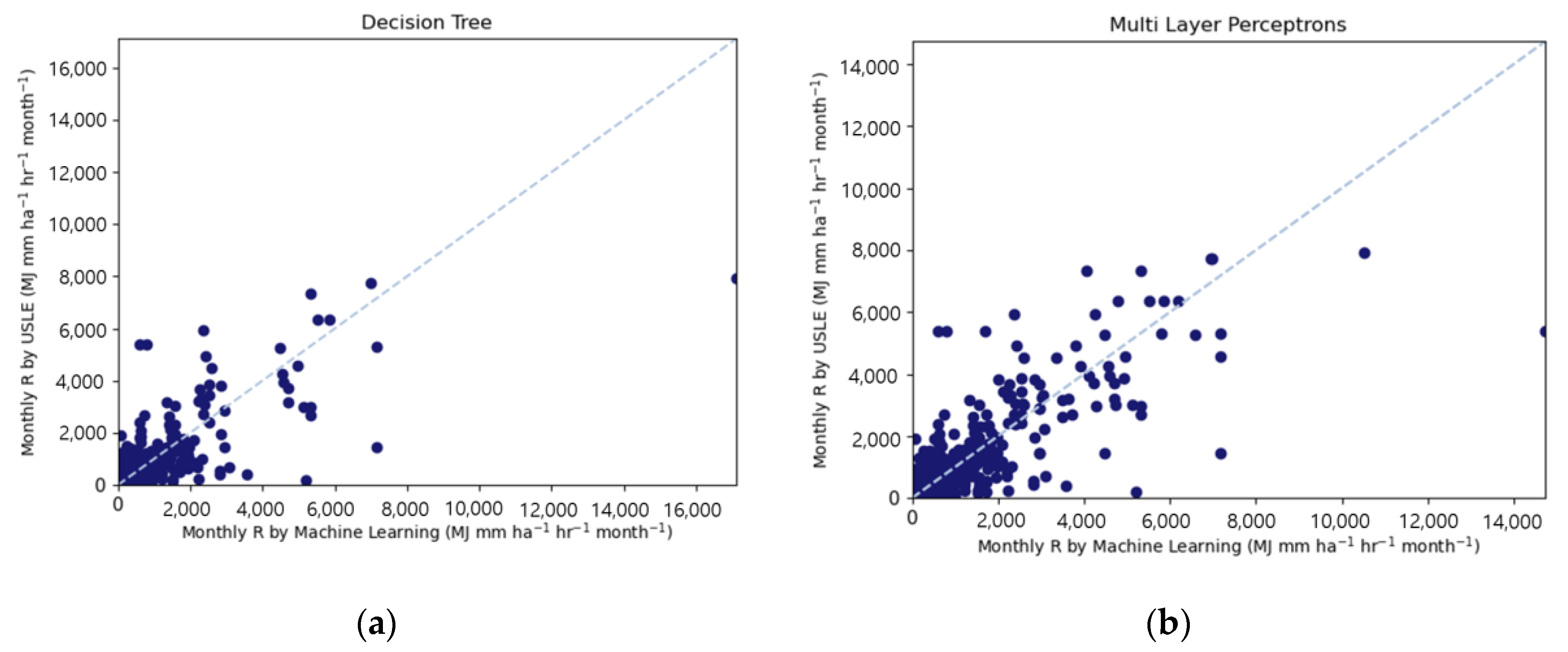
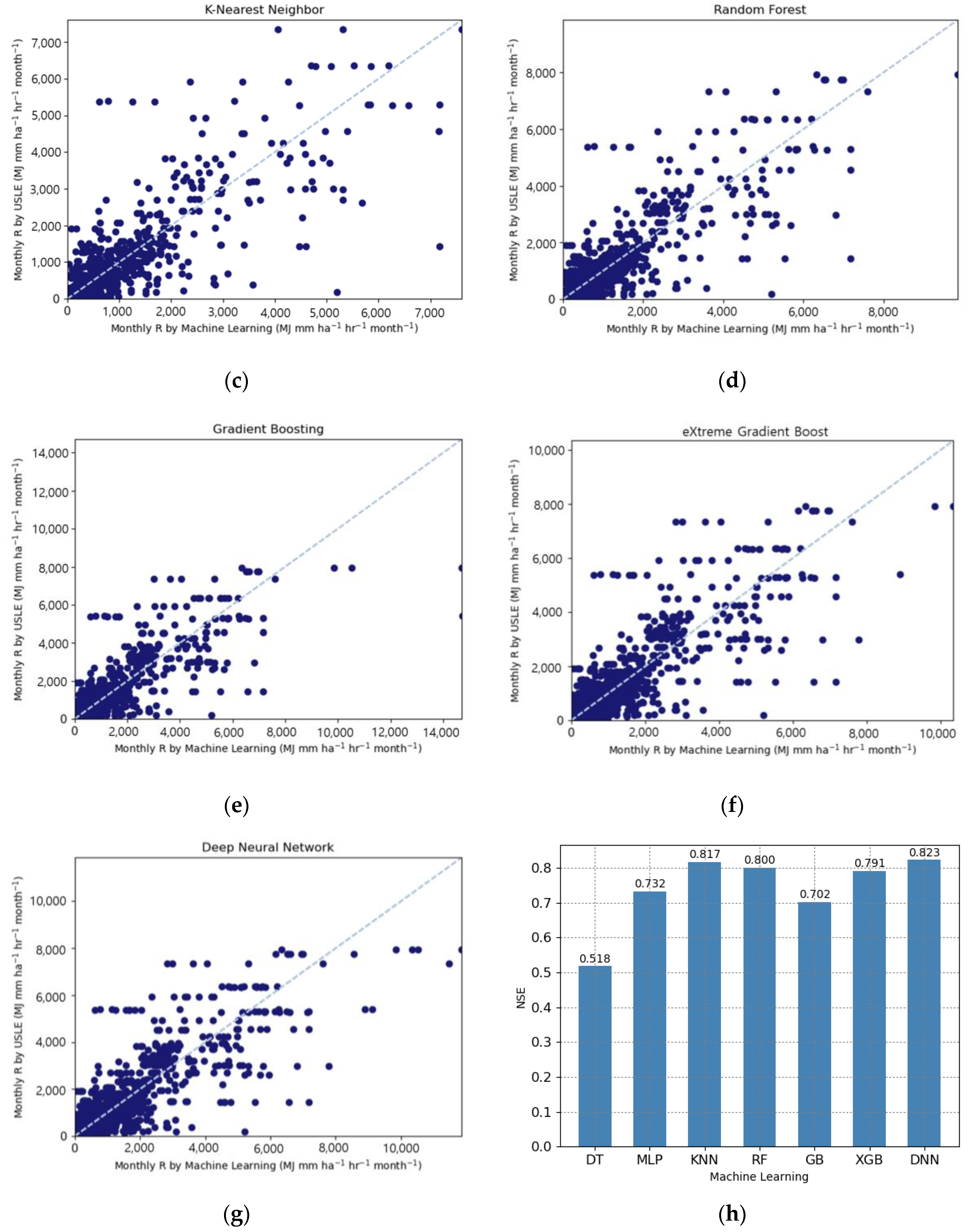
Table 5 shows the prediction accuracy results (NSE, RMSE, MAE, R2) of seven machine learning models, by comparing the predicted R-factor. The results from the Deep Neural Network (DNN) showed the highest prediction accuracy with NSE 0.823, RMSE 398.623 MJ mm ha−1 h−1 month−1, MAE 144.442 MJ mm ha−1 h−1 month−1, and R2 0.840.
When comparing the results of DNN and the other machine learning models (Decision Tree, Random Forest, K-Nearest Neighbors, Multilayer Perceptron, Gradient Boosting, and eXtreme Gradient Boost), we can see that DNN provided more accurate prediction results over other machine learning algorithms. Moreover, the highest value of NSE, RMSE, MAE, and R2 was found when the DNN was employed for the prediction R-factor values.
DNN had been proven for its good performance in a number of studies about the environment. In the study conducted by Liu et al. [59], the DNN showed better results, compared with results obtained by other machine learning algorithms, in predicting streamflow at Yangtze River. Nhu et al. [60] reported the DNN has the most impactful method in machine learning for the prediction of landslide susceptibility compared to other machine learning such as decision trees and logistic regression. In the study by Lee et al. [61], a DNN-based model showed good performance as a result of evaluating the heavy rain damage prediction compared to the recurrent neural network (RNN) in deep learning. Sit et al. [62] reported the DNN can be helpful in time-series forecasting for flood and support improving existing models. For these reasons, it has been shown that DNN performs better in various studies.
In this study, the second best-predicted model is the K-Nearest Neighbors (KNN). The result from the KNN model showed prediction accuracy with NSE 0.817, RMSE 405.327 MJ mm ha−1 h−1 month−1, MAE 149.923 MJ mm ha−1 h−1 month−1, and R2 0.794 which indicates that the KNN is the most effective, aside from DNN, in predicting R-factor. According to Kim et al. [63], KNN has good performance results in predicting the influent flow rate and four water qualities like chemical oxygen demand (COD), suspended solids (SS), total nitrogen (TN), and total phosphorus (TP) at a wastewater treatment plant.
On the other hand, Decision Tree has prediction accuracy, with NSE 0.518, RMSE 657.672 MJ mm ha−1 h−1 month−1, MAE 217.408, MJ mm ha−1 month-−1, and R2 0.626. This means that Decision Tree is less predictable than other machine learning models (Random Forest, K-Nearest Neighbors, Multilayer Perceptron, Gradient Boosting, eXtreme Gradient Boost, and Deep Neural Network). Hong et al. [37] also reported Decision Tree has less accuracy for the prediction of dam inflow compared to other machine learning models (Decision tree, Multilayer perceptron, Random forest, Gradient boosting, Convolutional neural network, and Recurrent neural network-long short-term memory).
Figure 5 shows the scattering graphs of the R-factors predicted by the seven machine learning models and calculated by the USLE method. All machine learning results represent a rather distracting correlation with less agreement. However, in Figure 5h, the Deep Neural Network algorithms predicted USLE R values calculated using the method suggested by USLE users’ manual with higher accuracy, NSE value of 0.823.
Among the data, 80% of randomly selected data were trained, the model was created, and then the remaining 20% of data were used for the validation of the trained model. To prevent overfitting, the K-fold cross-validation was implemented for R2 as shown in Table 6. As a result of the five attempts of K-fold cross-validation, the DNN showed the best results with an average R2 of 0.783.
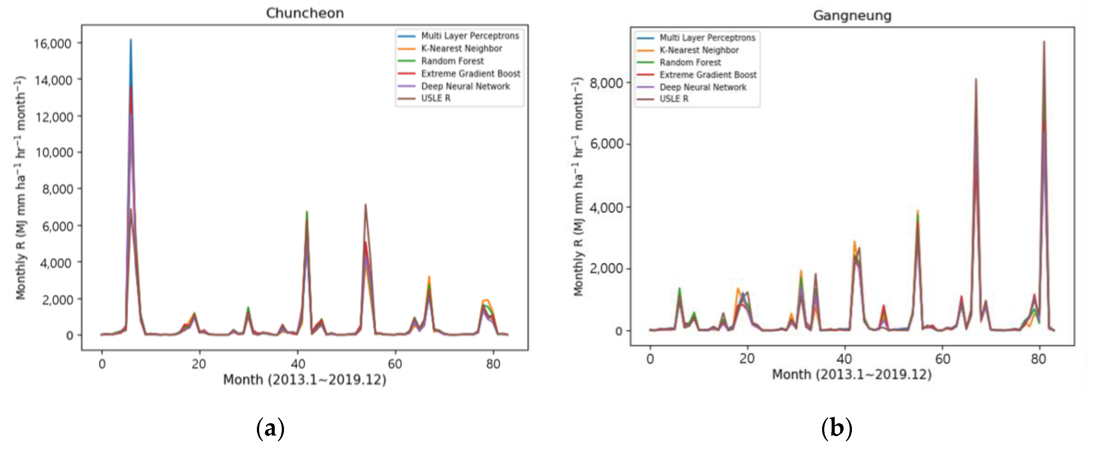
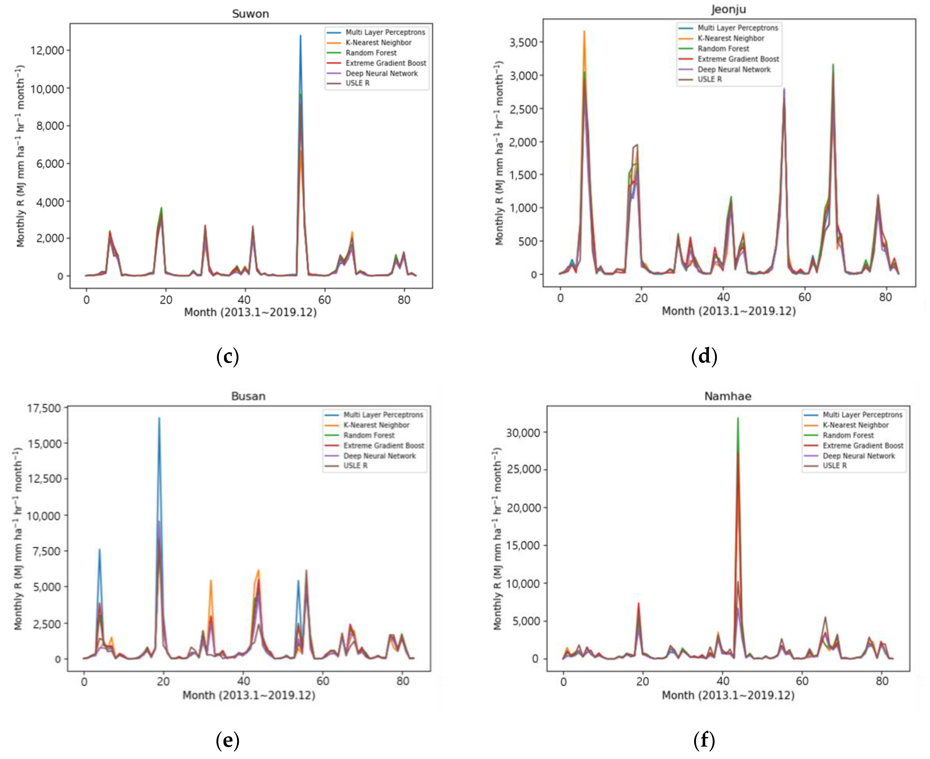
Figure 6 shows the results of the prediction of the five machine learning models (i.e., Multilayer Perceptron, K-Nearest Neighbor, Random Forest, eXtreme Gradient Boost, and Deep Neural Network) at six sites for the testing of the selected models, as well as the time series comparison graph for 2013–2019 of the monthly R-factor values calculated on the USLE basis. At most sites, it showed that the time series trend fits well with a pattern similar to the USLE calculation value. In particular, looking at the distribution in Figure 6b Gangneung, the value of 9303 MJ mm ha−1 h−1 month−1 in October 2019, which represented the peak value of the rainfall erosivity factor, was generally well predicted by all machine learning models. Among the models, the result of the Random Forest model estimated a similar value with 8133 MJ mm ha−1 h−1 month−1.
On the other hand, among six sites, the time series distribution values of the model prediction result in Busan showed a slightly different pattern from the USLE calculation R-factor. In particular, the result was overestimated as the values of 8241 MJ mm ha−1 h−1 month−1 in August 2014, and Multilayer Perceptron was almost twice overestimated at 16,725 MJ mm ha−1 h−1 month−1.
However, the Random Forest (8188 MJ mm ha−1 h−1 month−1) and eXtreme Gradient boost (8395 MJ mm ha−1 h−1 month−1) algorithms were predicting very similar values. Therefore, the machine learning results could be seen as good at predicting the peak value.
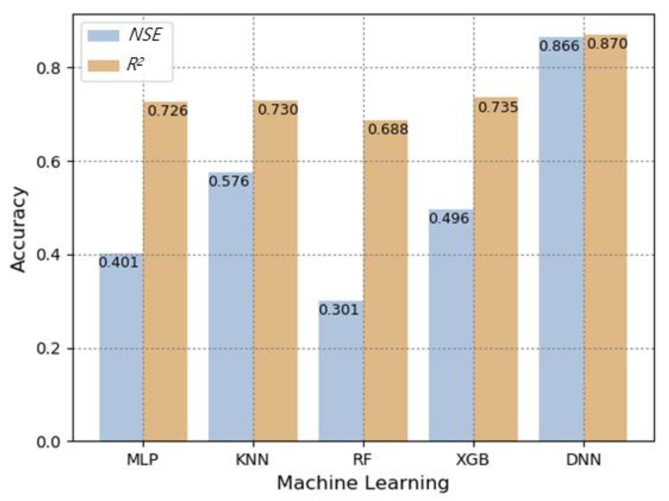
A comparison of the machine learning model accuracies of NSE and R2 of the test (validation) results at the six sites is shown in Figure 7. All five models had a coefficient of determination of 0.69 or higher, and the simulated values of the USLE method calculation and machine learning models showed high accuracy prediction. However, compared to Deep Neural Network, the NSE results of the four models (Multilayer Perceptron, K-Nearest Neighbor, Random Forest, eXtreme Gradient Boost) were less than 0.58, and the Deep Neural Network model showed 0.87 in both NSE and R2. Therefore, the monthly average value of the R-factor, predicted by the DNN would be a good candidate algorithm for USLE R factor prediction (Table 5 and Figure 7).
Table 7 shows average monthly rainfall erosivity factor values at the six sites for testing, Chuncheon, Gangneung, Suwon, Jeonju, Busan, and Namhae, along with the USLE calculation and Deep Neural Network (DNN) prediction.
Among average annual vales, the results for Busan showed a good performance with the Deep Neural Network (DNN) resulting in the average annual value of the rainfall erosivity factor of 257 MJ mm ha−1 h−1 year−1 difference over the USLE calculation result. In the case of Chuncheon, DNN also showed a good performance with an average annual rainfall erosivity factor difference of 298 MJ mm ha−1 h−1 year−1 difference over the USLE calculation result. On the other hand, the USLE calculation results for Namhae showed an average annual value of the rainfall erosivity factor difference of 3361 MJ mm ha−1 h−1 year−1 greater than the DNN result.
This is because, in the case of Namhae, the rainfall tendency lasted for a long period in the dry season from February to June compared to the other testing sites like Chuncheon, Gangneung, Suwon, Jeonju, and Busan. Moreover, the monthly R-factor calculation of Namhae in dry seasons was two to four times more than other testing sites. In particular, the monthly R-factor for February in Namhae figure being about five times higher than the monthly R-factor in Busan. This means that if the single set of learning data has a huge deviation or variation from other sets, it may result in the uncertainty of the entire result data. Therefore, the monthly R-factor of Namhae in the dry season from is containing uncertainty. In the future study, when predicting the R-factor of the Namhae, DNN model analysis will be implemented in consideration of rainfall trends by supplement the historical rainfall data.
R-factor can be calculated by machine learning algorithms with high accuracy and time benefit. The spatio-temporal calculation of the rainfall erosivity factor using machine learning techniques can be utilized for the estimation of the soil erosion due to rainfall at the target value. The DNN will be incorporated into the WERM website in the near future after further validation.
4. Conclusions
The main objective of this study is to develop machine learning models to predict monthly R-factor values which are comparable with those calculated by the USLE method. For this, we calculated R-factor using 1-min interval rainfall data for improved accuracy of the target value. The machine learning and deep learning models used in this study were Decision Tree, K-Nearest Neighbors, Multilayer Perceptron, Random forest, Gradient boosting, eXtreme Gradient boost, and Deep Neural Network. All of the models except Decision Tress showed NSE and R2 values of 0.7 or more, which means that most of the machine learning models showed high accuracy for predicting the R-factor. Among these, the Deep Neural Network (DNN) showed the best performance. As a result of the validation with 20% randomly selected data, DNN, among the seven models, showed the greatest prediction accuracy results with NSE 0.823, RMSE 398.623 MJ mm ha−1 h−1 month−1, MAE 144.442 MJ mm ha−1 h−1 month−1, and R2 0.840. Furthermore, the DNN developed in this study was tested for six sites (Chuncheon, Gangneung, Suwon, Jeonju, Busan, and Namhae) in S. Korea to demonstrate a trained model performance with NSE and R2 of both 0.87. As a result of the comparative analysis of R-factor prediction through various models, the DNN was proven to be the best model for R-factor prediction in S. Korea with readily available rainfall data. The model accuracy and simplicity of machine learning and deep learning models insist that the models could replace traditional ways of calculating/estimating USLE R-factor values.
We found that the maximum 30 min intensity derived from 1-min interval rainfall data in this study is more accurate than that estimated from previous research. These methods can provide more accurate monthly, yearly, and event-based USLE R-factor for the entire period. Moreover, if the user has input data (month, the total amount of monthly precipitation, maximum daily precipitation, maximum hourly precipitation) as described in Table 3, the monthly R-factor can be easily calculated for the 50 specific stations in S. Korea by using the machine and deep learning models. Since the updated R-factor in this study reflected the recent rainfall data, which have high variability, it can improve the accuracy of the usage of the previous R-factor proposed by the Korean Ministry of Environment [64] for future study. The results from this study can help the policymakers to update their guideline (Korean Ministry of Environment) [64] regarding the updated version of R-factors values for S. Korea.
It is expected that it will be used not only to calculate soil erosion risk but also to establish soil conservation plans and identify areas at risk of soil disasters by calculating rainfall erosivity factors at the desired temporal-spatial areas more easily and quickly.
However, this study evaluated the R-factor using machine learning models in S. Korean territory, under the monsoon region. Although deep learning models such as Deep Neural Network’s applicability in S. Korea has been confirmed in this study, few studies have investigated and benchmarked the performances of a Deep Neural Network model-based USLE R-factor prediction trained. Therefore, future studies should be carried out for the diverse conditions of the other countries such as European countries, the United States, and African countries to broaden the applicability of machine learning technology in USLE R-factor (erosivity factor) analysis.
Author Contributions
Conceptualization and methodology: J.L., J.E.Y., J.K., and K.J.L.; formal analysis: J.H.B. and D.L.; data curation: J.L., J.H., and S.L.; writing—original draft preparation: J.L.; writing—review and editing: J.K.; supervision: K.J.L. All authors have read and agreed to the published version of the manuscript.
Funding
This research was funded by the Ministry of Environment of Korea as The SS (Surface Soil conservation and management) projects [2019002820003].
Institutional Review Board Statement
Not applicable.
Informed Consent Statement
Not applicable.
Data Availability Statement
Not applicable.
Conflicts of Interest
The authors declare no conflict of interest.
References
- Diodato, N.; Bellocchi, G. Estimating monthly (R) USLE climate input in a Mediterranean region using limited data. J. Hydrol. 2007, 345, 224–236. [Google Scholar] [CrossRef]
- Fu, B.J.; Zhao, W.W.; Chen, L.D.; Liu, Z.F.; Lü, Y.H. Eco-hydrological effects of landscape pattern change. Landsc. Ecol. Eng. 2005, 1, 25–32. [Google Scholar] [CrossRef]
- Renschler, C.S.; Harbor, J. Soil erosion assessment tools from point to regional scales the role of geomorphologists in land management research and implementation. Geomorphology 2002, 47, 189–209. [Google Scholar] [CrossRef]
- Christensen, O.; Yang, S.; Boberg, F.; Maule, C.F.; Thejll, P.; Olesen, M.; Drews, M.; Sorup, H.J.D.; Christensen, J. Scalability of regional climate change in Europe for high-end scenarios. Clim. Res. 2015, 64, 25. [Google Scholar] [CrossRef] [Green Version]
- Stocker, T.; Gin, D.; Plattner, G.; Tignor, M.; Allen, S.; Boschung, J.; Nauels, A.; Xia, Y.; Bex, V.; Midgley, P.E. Climate Change 2013: The Physical Science Basis: Contribution of Working Group I to the Fifth Assessment Report of the Intergovernmental Panel on Climate Change; Cambridge University Press: Cambridge, UK; New York, NY, USA, 2013; p. 1535. [Google Scholar]
- Achite, M.; Buttafuoco, G.; Toubal, K.A.; Lucà, F. Precipitation spatial variability and dry areas temporal stability for different elevation classes in the Macta basin (Algeria). Environ. Earth Sci. 2017, 76, 458. [Google Scholar] [CrossRef]
- Shi, Z.; Yan, F.; Li, L.; Li, Z.; Cai, C. Interrill erosion from disturbed and undisturbed samples in relation to topsoil aggregate stability in red soils from subtropical China. Catena 2010, 81, 240–248. [Google Scholar] [CrossRef]
- Kinnell, P.I.A.; Wang, J.; Zheng, F. Comparison of the abilities of WEPP and the USLE-M to predict event soil loss on steep loessal slopes in China. Catena 2018, 171, 99–106. [Google Scholar] [CrossRef]
- Lee, J.; Park, Y.S.; Kum, D.; Jung, Y.; Kim, B.; Hwang, S.J.; Kim, H.B.; Kim, C.; Lim, K.J. Assessing the effect of watershed slopes on recharge/baseflow and soil erosion. Paddy Water Environ. 2014, 12, 169–183. [Google Scholar] [CrossRef]
- Pandey, A.; Himanshu, S.; Mishra, S.K.; Singh, V. hysically based soil erosion and sediment yield models revisited. Catena 2016, 147, 595–620. [Google Scholar] [CrossRef]
- Sigler, W.A.; Ewing, S.A.; Jones, C.A.; Payn, R.A.; Miller, P.; Maneta, M. Water and nitrate loss from dryland agricultural soils is controlled by management, soils, and weather. Agric. Ecosyst. Environ. 2020, 304, 107158. [Google Scholar] [CrossRef]
- Lucà, F.; Buttafuoco, G.; Terranova, O. GIS and Soil. In Comprehensive Geographic Information Systems; Huang, B., Ed.; Elsevier: Oxford, UK, 2018; Volume 2, pp. 37–50. [Google Scholar]
- Arnold, J.G.; Srinivasan, R.; Muttiah, R.S.; Williams, J.R. Large area hydrologic modeling and assessment part I: Model development1. J. Am. Water Resour. Assoc. 1998, 34, 73–89. [Google Scholar] [CrossRef]
- Morgan, R.P.C.; Quinton, J.N.; Smith, R.E.; Govers, G.; Poesen, J.W.A.; Auerswald, K.; Chisci, G.; Torri, D.; Styczen, M.E. The European soil erosion model (EUROSEM): A dynamic approach for predicting sediment transport from fields and small catchments. Earth Surf. Process. Landf. 1998, 23, 527–544. [Google Scholar] [CrossRef]
- Flanagan, D.; Nearing, M. USDA-water erosion prediction project: Hillslope profile and watershed model documentation. NSERL Rep. 1995, 10, 1–12. [Google Scholar]
- Lim, K.J.; Sagong, M.; Engel, B.A.; Tang, Z.; Choi, J.; Kim, K.S. GIS-based sediment assessment tool. Catena 2005, 64, 61–80. [Google Scholar] [CrossRef]
- Young, R.A.; Onstad, C.; Bosch, D.; Anderson, W. AGNPS: A nonpoint-source pollution model for evaluating agricultural watersheds. J. Soil Water Conserv. 1989, 44, 168–173. [Google Scholar]
- Wischmeier, W.H.; Smith, D.D. Predicting Rainfall Erosion Losses: A Guide to Conservation Planning; Department of Agriculture, Science, and Education Administration: Wahsington, DC, USA, 1978; pp. 1–67.
- Renard, K.G.; Foster, G.R.; Weesies, G.A.; McCool, D.K.; Yorder, D.C. Predicting Soil Erosion by Water: A Guide to Conservation Planning with the Revised Universal Soil Loss Equation (RUSLE). In Agriculture Handbook; U.S. Department of Agriculture: Washington, DC, USA, 1997; Volume 703. [Google Scholar]
- Kinnell, P.I.A. Comparison between the USLE, the USLE-M and replicate plots to model rainfall erosion on bare fallow areas. Catena 2016, 145, 39–46. [Google Scholar] [CrossRef]
- Bagarello, V.; Stefano, C.D.; Ferro, V.; Pampalone, V. Predicting maximum annual values of event soil loss by USLE-type models. Catena 2017, 155, 10–19. [Google Scholar] [CrossRef]
- Park, Y.S.; Kim, J.; Kim, N.W.; Kim, S.J.; Jeong, J.; Engel, B.A.; Jang, W.; Lim, K.J. Development of new R C and SDR modules for the SATEEC GIS system. Comput. Geosci. 2010, 36, 726–734. [Google Scholar] [CrossRef]
- Yu, N.Y.; Lee, D.J.; Han, J.H.; Lim, K.J.; Kim, J.; Kim, H.; Kim, S.; Kim, E.S.; Pakr, Y.S. Development of ArcGIS-based model to estimate monthly potential soil loss. J. Korean Soc. Agric. Eng. 2017, 59, 21–30. [Google Scholar]
- Park, C.W.; Sonn, Y.K.; Hyun, B.K.; Song, K.C.; Chun, H.C.; Moon, Y.H.; Yun, S.G. The redetermination of USLE rainfall erosion factor for estimation of soil loss at Korea. korean J. Soil Sci. Fert. 2011, 44, 977–982. [Google Scholar] [CrossRef] [Green Version]
- Panagos, P.; Ballabio, C.; Borrelli, P.; Meusburger, K. Spatio-temporal analysis of rainfall erosivity and erosivity density in Greece. Catena 2016, 137, 161–172. [Google Scholar] [CrossRef]
- Sholagberu, A.T.; Mustafa, M.R.U.; Yusof, K.W.; Ahmad, M.H. Evaluation of rainfall-runoff erosivity factor for Cameron highlands, Pahang, Malaysia. J. Ecol. Eng. 2016, 17. [Google Scholar] [CrossRef] [Green Version]
- Risal, A.; Bhattarai, R.; Kum, D.; Park, Y.S.; Yang, J.E.; Lim, K.J. Application of Web Erosivity Module (WERM) for estimation of annual and monthly R factor in Korea. Catena 2016, 147, 225–237. [Google Scholar] [CrossRef]
- Risal, A.; Lim, K.J.; Bhattarai, R.; Yang, J.E.; Noh, H.; Pathak, R.; Kim, J. Development of web-based WERM-S module for estimating spatially distributed rainfall erosivity index (EI30) using RADAR rainfall data. Catena 2018, 161, 37–49. [Google Scholar] [CrossRef]
- Lucà, F.; Robustelli, G. Comparison of logistic regression and neural network models in assessing geomorphic control on alluvial fan depositional processes (Calabria, southern Italy). Environ. Earth Sci. 2020, 79, 39. [Google Scholar] [CrossRef]
- Noymanee, J.; Theeramunkong, T. Flood forecasting with machine learning technique on hydrological modeling. Preced. Comput. Sci. 2019, 156, 377–386. [Google Scholar] [CrossRef]
- Vantas, K.; Sidiropoulos, E.; Evangelides, C. Rainfall erosivity and Its Estimation: Conventional and Machine Learning Methods. In Soil Erosion—Rainfall Erosivity and Risk Assessment; Intechopen: London, UK, 2019. [Google Scholar]
- Zhao, G.; Pang, B.; Xu, Z.; Peng, D.; Liang, X. Assessment of urban flood susceptibility using semi supervised machine learning model. Sci. Total Environ. 2019, 659, 940–949. [Google Scholar] [CrossRef] [PubMed]
- Vu, D.T.; Tran, X.L.; Cao, M.T.; Tran, T.C.; Hoang, N.D. Machine learning based soil erosion susceptibility prediction using social spider algorithm optimized multivariate adaptive regression spline. Measurement 2020, 164, 108066. [Google Scholar] [CrossRef]
- Xiang, Z.; Demir, I. Distributed long-term hourly streamflow predictions using deep learning—A case study for state of Iowa. Environ. Modeling Softw. 2020, 131, 104761. [Google Scholar] [CrossRef]
- Renard, K.G.; Foster, G.R.; Weesies, G.A.; Porter, J.P. RUSLE: Revised universal soil loss equation. J. Soil Water Conserv. 1991, 46, 30–33. [Google Scholar]
- Alpaydin, E. Introduction to Machine Learning, 4th ed.; MIT Press: Cambridge, MA, USA, 2014; pp. 1–683. [Google Scholar]
- Hong, J.; Lee, S.; Bae, J.H.; Lee, J.; Park, W.J.; Lee, D.; Kim, J.; Lim, K.J. Development and evaluation of the combined machine learning models for the prediction of dam inflow. Water 2020, 12, 2927. [Google Scholar] [CrossRef]
- Wang, L.; Guo, M.; Sawada, K.; Lin, J.; Zhang, J.A. Comparative Study of Landslide Susceptibility Maps using Logistic Regression, Frequency Ratio, Decision Tree, Weights of Evidence and Artificial Neural Network. Geosci. J. 2016, 20, 117–136. [Google Scholar] [CrossRef]
- Safavian, S.R.; Landgrebe, D. A survey of decision tree classifier methodology. IEEE Trans. Syst. Man Cybern. 1991, 21, 660–674. [Google Scholar] [CrossRef] [Green Version]
- Breiman, L. Random forests. Mach. Learn. 2001, 45, 5–32. [Google Scholar] [CrossRef] [Green Version]
- Moon, J.; Park, S.; Hwang, E. A multilayer perceptron-based electric load forecasting scheme via effective recovering missing data. Kips Trans. Softw. Data Eng. 2019, 8, 67–78. [Google Scholar]
- Bae, J.H.; Han, J.; Lee, D.; Yang, J.E.; Kim, J.; Lim, K.J.; Neff, J.C.; Jang, W.S. Evaluation of Sediment Trapping Efficiency of Vegetative Filter Strips Using Machine Learning Models. Sustainability 2019, 11, 7212. [Google Scholar] [CrossRef] [Green Version]
- Qu, W.; Li, J.; Yang, L.; Li, D.; Liu, S.; Zhao, Q.; Qi, Y. Short-term intersection Traffic flow forecasting. Sustainability 2020, 12, 8158. [Google Scholar] [CrossRef]
- Yao, Z.; Ruzzo, W.L. A regression-based K nearest neighbor algorithm for gene function prediction from heterogeneous data. BMC Bioinform. 2006, 7, S11. [Google Scholar] [CrossRef] [Green Version]
- Ooi, H.L.; Ng, S.C.; Lim, E. ANO detection with K-Nearest Neighbor using minkowski distance. Int. J. Process. Syst. 2013, 2, 208–211. [Google Scholar] [CrossRef]
- Natekin, A.; Knoll, A. Gradient boosting machines, a tutorial. Front. Neurorobot. 2013, 7, 21. [Google Scholar] [CrossRef] [Green Version]
- Friedman, J.H. Greedy function approximation: A gradient boosting machine. Ann. Stat. 2001, 29, 1189–1232. [Google Scholar] [CrossRef]
- Ngarambe, J.; Irakoze, A.; Yun, G.Y.; Kim, G. Comparative Performance of Machine Learning Algorithms in the Prediction of Indoor Daylight Illuminances. Sustainability 2020, 12, 4471. [Google Scholar] [CrossRef]
- Georganos, S.; Grippa, T.; Vanhuysse, S.; Lennert, M.; Shimoni, M. Very high resolution object-based land use–land cover urban classification using extreme gradient boosting. IEEE Geosci. Remote Sens. Lett. 2018, 15, 607–611. [Google Scholar] [CrossRef] [Green Version]
- Babajide Mustapha, I.; Saeed, F. Bioactive molecule prediction using extreme gradient boosting. Molecules 2016, 21, 983. [Google Scholar] [CrossRef] [Green Version]
- Lavecchia, A. Machine-learning approaches in drug discovery: Methods and applications. Drug Discov. Today. 2015, 20, 318–331. [Google Scholar] [CrossRef] [Green Version]
- Rumelhart, D.E.; Hinton, G.E.; Williams, R.J. Learning representations by back-propagating errors. Nature 1986, 323, 533–536. [Google Scholar] [CrossRef]
- Wang, Q.; Wang, S. Machine learning-based water level prediction in Lake Erie. Water 2020, 12, 2654. [Google Scholar] [CrossRef]
- Siniscalchi, S.M.; Yu, D.; Deng, L.; Lee, C.H. Exploiting deep neural networks for detection-based speech recognition. Neurocomputing 2013, 106, 148–157. [Google Scholar] [CrossRef]
- Hinton, G.E.; Osindero, S.; Teh, Y.W. A fast learning algorithm for deep belief nets. Neural Comput. 2006, 18, 1527–1554. [Google Scholar] [CrossRef]
- Cancelliere, A.; Di Mauro, G.; Bonaccorso, B.; Rossi, G. Drought forecasting using the standardized precipitation index. Water Resour. Manag. 2007, 21, 801–819. [Google Scholar] [CrossRef]
- Legates, D.R.; McCabe, G.J., Jr. Evaluating the use of “goodness-of-fit” measures in hydrologic and hydroclimatic model validation. Water Resour. Res. 1999, 35, 233–241. [Google Scholar] [CrossRef]
- Moghimi, M.M.; Zarei, A.R. Evaluating the performance and applicability of several drought indices in arid regions. Asia-Pac. J. Atmos. Sci. 2019, 1–17. [Google Scholar] [CrossRef]
- Liu, D.; Jiang, W.; Wang, S. Streamflow prediction using deep learning neural network: A case study of Yangtze River. Inst. Electr. Electron. Eng. 2020, 8, 90069–90086. [Google Scholar] [CrossRef]
- Nhu, V.; Hoang, N.; Nguyen, H.; Ngo, P.T.T.; Bui, T.T.; Hoa, P.V.; Samui, P.; Bui, D.T. Effectiveness assessment of Keras based deep learning with different robust optimization algorithms for shallow landslide susceptibility mapping at tropical area. Catena 2020, 188, 104458. [Google Scholar] [CrossRef]
- Lee, K.; Choi, C.; Shin, D.H.; Kim, H.S. Prediction of heavy rain damage using deep learning. Water 2020, 12, 1942. [Google Scholar] [CrossRef]
- Sit, M.A.; Demir, I. Decentralized flood forecasting using deep neural networks. arXiv 2019, arXiv:1902.02308. [Google Scholar]
- Kim, M.; Kim, Y.; Kim, H.; Piao, W. Evaluation of the k-nearest neighbor method for forecasting the influent characteristics of wastewater treatment plant. Front. Environ. Sci. Eng. 2015, 10, 299–310. [Google Scholar] [CrossRef]
- Korea Ministry of Environment. Notice Regarding Survey of Topsoil Erosion; Ministry of Environment: Seoul, Korea, 2012; pp. 1–41.
Figure 1.
Study procedures.

Figure 2.
Weather stations in the study area.

Figure 3.
Illustration of the proposed Deep Neural Network (DNN) for rainfall erosivity (R-factor) prediction.
Figure 3.
Illustration of the proposed Deep Neural Network (DNN) for rainfall erosivity (R-factor) prediction.

Figure 4.
Spatial distribution of monthly R-factor calculated by USLE, using rainfall data from 50 weather stations for the period 2013–2019.
Figure 4.
Spatial distribution of monthly R-factor calculated by USLE, using rainfall data from 50 weather stations for the period 2013–2019.

Figure 5.
Comparison of (a) Decision Tree, (b) Multilayer Perceptron, (c) K-Nearest Neighbor, (d) Random Forest, (e) Gradient Boosting, (f) eXtreme Gradient Boost, and (g) Deep Neural Network calculated R-factor with validation data, and (h) comparison of machine learning accuracy.
Figure 5.
Comparison of (a) Decision Tree, (b) Multilayer Perceptron, (c) K-Nearest Neighbor, (d) Random Forest, (e) Gradient Boosting, (f) eXtreme Gradient Boost, and (g) Deep Neural Network calculated R-factor with validation data, and (h) comparison of machine learning accuracy.


Figure 6.
The comparisons of forecasting results of R-factor using machine learning in (a) Chuncheon, (b) Gangneung, (c) Suwon, (d) Jeonju, (e) Busan, and (f) Namhae.
Figure 6.
The comparisons of forecasting results of R-factor using machine learning in (a) Chuncheon, (b) Gangneung, (c) Suwon, (d) Jeonju, (e) Busan, and (f) Namhae.


Figure 7.
Comparison of prediction accuracy results by machine learning models in test sites.


Table 1.
Description of machine learning models.
| Machine Learning Models | Module | Function | Notation |
|---|---|---|---|
| Decision Tree | Sklearn.tree | DecisionTreeRegressor | DT |
| Random Forest | Sklearn.ensemble | RandomForestRegressor | RF |
| K-Nearest Neighbors | Sklearn.neighbors | KNeighborsRegressor | KN |
| Gradient Boosting | Sklearn.ensemble | GradientBoostingRegressor | GB |
| eXtreme Gradient Boost | xgboost.xgb | XGBRegressor | XGB |
| Multilayer Perceptron | Sklearn, neural_network | MLPRegressor | MLP |
| Deep Neural Network | Keras.models.Sequential | Dense, Dropout | DNN |
Table 2.
Critical hyperparameters in machine learning models.
| Machine Learning Models | Hyperparameter |
|---|---|
| Decision Tree | criterion = “entropy”, min_samples_split = 2 |
| Random Forest | n_estimators = 52, min_samples_leaf = 1 |
| K-Nearest Neighbors | n_neighbors = 3, weights = ‘uniform’, metric = ‘minkowski’ |
| Gradient Boosting | learning_rate = 0.01, min_samples_split = 4 |
| eXtreme Gradient Boost | Booster = ‘gbtree’, max_depth = 10 |
| Multilayer Perceptron | hidden_layer_sizes = (50,50,50), activation = “relu”, solver = ‘adam’ |
| Deep Neural Network | kernel_initializer = ‘normal’, activation = “relu” |
Table 3.
The input data for machine learning models.
| Description | Count | Mean | std | Min | 25% | 50% | 75% | Max | ||
|---|---|---|---|---|---|---|---|---|---|---|
| Input variable | month | month (1~12) | 4087 | 6.49 | 3.45 | 1 | 3 | 6 | 9 | 12 |
| m_sum_r | the total amount of monthly precipitation | 4087 | 96.45 | 97.01 | 0 | 30.90 | 66.20 | 126.15 | 1009.20 | |
| d_max_r | maximum daily precipitation | 4087 | 39.39 | 38.10 | 0 | 14.50 | 27.10 | 51.35 | 384.30 | |
| h_max_r | maximum hourly precipitation | 4087 | 11.84 | 12.69 | 0 | 4.00 | 7.50 | 15.50 | 197.50 | |
| Output variable | R-factor | R-factor | 4087 | 419.10 | 1216.79 | 0 | 15.99 | 77.84 | 326.24 | 43,586.61 |
Table 4.
Monthly R-factor calculated by the Universal Soil Loss Equation (USLE).
| Station Number | Station Name | R-Factor (MJ mm ha−1 h−1 month−1) | R-Factor (MJ mm ha−1 h−1 year−1) | |||||||||||
|---|---|---|---|---|---|---|---|---|---|---|---|---|---|---|
| January | February | March | April | May | June | July | August | September | October | November | December | Annual | ||
| 90 | Sokcho | 21 | 29 | 32 | 95 | 47 | 159 | 1039 | 2860 | 368 | 494 | 507 | 44 | 5694 |
| 95 | Cheolwon | 2 | 37 | 30 | 119 | 257 | 235 | 5867 | 2769 | 403 | 239 | 65 | 24 | 10,046 |
| 98 | Dongducheon | 2 | 69 | 31 | 91 | 287 | 455 | 3031 | 1364 | 424 | 228 | 47 | 24 | 6053 |
| 100 | Daegwallyeong | 4 | 19 | 20 | 79 | 577 | 194 | 1472 | 1669 | 453 | 237 | 40 | 8 | 4772 |
| 106 | Donghae | 17 | 29 | 34 | 207 | 27 | 157 | 592 | 1317 | 469 | 1461 | 128 | 8 | 4447 |
| 108 | Seoul | 0 | 31 | 37 | 95 | 284 | 266 | 2813 | 988 | 191 | 90 | 50 | 16 | 4861 |
| 112 | Incheon | 3 | 50 | 69 | 83 | 224 | 192 | 2193 | 897 | 406 | 480 | 88 | 27 | 4712 |
| 114 | Wonju | 2 | 22 | 31 | 83 | 284 | 699 | 2654 | 999 | 303 | 65 | 40 | 8 | 5189 |
| 127 | Chungju | 4 | 36 | 22 | 79 | 171 | 270 | 2075 | 1240 | 909 | 117 | 38 | 17 | 4978 |
| 129 | Seosan | 7 | 72 | 50 | 135 | 147 | 562 | 747 | 635 | 330 | 146 | 127 | 42 | 3000 |
| 130 | Uljin | 86 | 16 | 47 | 292 | 24 | 227 | 590 | 470 | 360 | 2816 | 143 | 30 | 5100 |
| 133 | Daejeon | 8 | 47 | 50 | 182 | 72 | 602 | 1658 | 1293 | 494 | 181 | 96 | 24 | 4707 |
| 136 | Andong | 1 | 32 | 53 | 101 | 48 | 325 | 1142 | 808 | 368 | 176 | 33 | 14 | 3100 |
| 137 | Sangju | 6 | 18 | 67 | 105 | 45 | 361 | 1098 | 1143 | 420 | 273 | 51 | 19 | 3605 |
| 138 | Pohang | 7 | 46 | 106 | 139 | 40 | 233 | 417 | 1051 | 910 | 1478 | 51 | 23 | 4500 |
| 143 | Daegu | 1 | 8 | 57 | 80 | 67 | 313 | 548 | 1322 | 238 | 340 | 26 | 12 | 3013 |
| 152 | Ulsan | 15 | 36 | 122 | 141 | 154 | 287 | 751 | 1499 | 727 | 1709 | 77 | 74 | 5591 |
| 156 | Gwangju | 8 | 59 | 92 | 156 | 74 | 927 | 1249 | 2458 | 703 | 361 | 99 | 49 | 6236 |
| 165 | Mokpo | 15 | 112 | 117 | 227 | 177 | 630 | 1023 | 944 | 2094 | 493 | 85 | 127 | 6044 |
| 172 | Gochang | 12 | 24 | 137 | 151 | 77 | 399 | 1768 | 2235 | 614 | 273 | 77 | 21 | 5788 |
| 175 | Jindo | 18 | 43 | 231 | 559 | 511 | 598 | 738 | 1323 | 799 | 636 | 113 | 36 | 5606 |
| 201 | Ganghwa | 1 | 26 | 35 | 60 | 193 | 59 | 1922 | 1255 | 648 | 654 | 48 | 20 | 4921 |
| 203 | Icheon | 2 | 34 | 103 | 83 | 211 | 207 | 2284 | 1068 | 450 | 162 | 45 | 24 | 4673 |
| 212 | Hongcheon | 1 | 11 | 23 | 81 | 461 | 162 | 2220 | 934 | 223 | 51 | 29 | 8 | 4204 |
| 217 | Jeongseon | 1 | 20 | 18 | 75 | 117 | 126 | 2165 | 654 | 355 | 101 | 36 | 16 | 3686 |
| 221 | Jecheon | 3 | 26 | 21 | 90 | 158 | 265 | 1616 | 1162 | 405 | 80 | 43 | 12 | 3881 |
| 226 | Boeun | 8 | 19 | 42 | 106 | 62 | 482 | 2016 | 1102 | 583 | 163 | 77 | 15 | 4675 |
| 232 | Cheonan | 2 | 17 | 21 | 86 | 106 | 248 | 3408 | 1002 | 249 | 110 | 68 | 15 | 5333 |
| 235 | Boryeong | 5 | 73 | 47 | 142 | 127 | 322 | 878 | 849 | 1014 | 184 | 149 | 29 | 3820 |
| 238 | Guemsan | 5 | 17 | 52 | 154 | 48 | 483 | 1126 | 1059 | 447 | 148 | 37 | 17 | 3591 |
| 244 | Imsil | 3 | 9 | 83 | 106 | 67 | 369 | 2329 | 1416 | 632 | 224 | 44 | 16 | 5297 |
| 245 | Jeongeup | 11 | 18 | 106 | 160 | 265 | 318 | 1679 | 1930 | 521 | 207 | 46 | 27 | 5287 |
| 247 | Namwon | 8 | 19 | 78 | 159 | 52 | 704 | 2988 | 2304 | 479 | 586 | 88 | 49 | 7512 |
| 248 | Jangsu | 5 | 34 | 85 | 151 | 80 | 246 | 1997 | 1812 | 715 | 308 | 53 | 30 | 5516 |
| 251 | Gochanggoon | 7 | 14 | 127 | 191 | 69 | 352 | 1448 | 2066 | 521 | 175 | 37 | 23 | 5029 |
| 252 | Younggwang | 7 | 15 | 130 | 178 | 114 | 292 | 994 | 2008 | 596 | 491 | 63 | 39 | 4928 |
| 253 | Ginhae | 7 | 43 | 220 | 200 | 339 | 385 | 1036 | 1600 | 1216 | 734 | 44 | 48 | 5872 |
| 254 | Soonchang | 4 | 14 | 93 | 194 | 89 | 456 | 1724 | 1304 | 629 | 363 | 58 | 16 | 4945 |
| 259 | Gangjin | 10 | 34 | 204 | 344 | 425 | 666 | 1156 | 9781 | 903 | 444 | 187 | 18 | 14,170 |
| 261 | Haenam | 10 | 15 | 223 | 206 | 177 | 595 | 965 | 1142 | 650 | 1250 | 83 | 91 | 5406 |
| 263 | Uiryoong | 4 | 24 | 121 | 184 | 156 | 334 | 629 | 1961 | 805 | 643 | 39 | 36 | 4936 |
| 266 | Gwangyang | 8 | 76 | 120 | 218 | 591 | 686 | 827 | 2488 | 2195 | 555 | 86 | 73 | 7924 |
| 271 | Bonghwa | 0 | 9 | 36 | 86 | 95 | 415 | 1154 | 706 | 327 | 98 | 28 | 13 | 2968 |
| 273 | Mungyeong | 7 | 18 | 54 | 139 | 102 | 331 | 1724 | 742 | 529 | 180 | 61 | 21 | 3908 |
| 278 | Uiseong | 1 | 6 | 69 | 101 | 74 | 220 | 632 | 647 | 326 | 106 | 31 | 7 | 2220 |
| 279 | Gumi | 3 | 12 | 68 | 103 | 95 | 380 | 1296 | 1442 | 554 | 364 | 32 | 14 | 4363 |
| 281 | Yeongcheon | 2 | 11 | 81 | 162 | 52 | 316 | 1259 | 1082 | 409 | 230 | 28 | 12 | 3643 |
| 283 | Gyeongju | 3 | 11 | 53 | 101 | 55 | 125 | 573 | 759 | 681 | 686 | 21 | 13 | 3081 |
| 284 | Geochang | 3 | 17 | 54 | 105 | 60 | 434 | 1184 | 1491 | 619 | 2246 | 33 | 55 | 6299 |
| 285 | Hapcheon | 2 | 22 | 57 | 173 | 105 | 700 | 1114 | 1646 | 810 | 676 | 47 | 24 | 5378 |
Table 5.
Prediction accuracy results of seven machine learning models.
| Machine Learning Models | NSE | RMSE (MJ mm ha-−1 h−1 month−1) | MAE (MJ mm ha-−1 h−1 month−1) | R2 |
|---|---|---|---|---|
| Decision Tree | 0.518 | 657.672 | 217.408 | 0.626 |
| Multilayer Perceptron | 0.732 | 490.055 | 158.847 | 0.783 |
| K-Nearest Neighbors | 0.817 | 405.327 | 149.923 | 0.794 |
| Random Forest | 0.800 | 423.345 | 148.147 | 0.799 |
| Gradient Boosting | 0.702 | 516.956 | 161.259 | 0.722 |
| eXtreme Gradient Boost | 0.791 | 433.230 | 159.275 | 0.788 |
| Deep Neural Network | 0.823 | 398.623 | 144.442 | 0.840 |
Table 6.
K-fold cross validation results of seven machine learning models.
| Fold | Coefficient of Determination (R2) | ||||||
|---|---|---|---|---|---|---|---|
| Decision Tree | Multi-Layer Perceptron | K-Nearest Neighbors | Random Forest | Gradient Boosting | eXtreme Gradient Boost | Deep Neural Network | |
| 1 | 0.631 | 0.781 | 0.818 | 0.817 | 0.730 | 0.801 | 0.821 |
| 2 | 0.598 | 0.806 | 0.705 | 0.686 | 0.648 | 0.737 | 0.733 |
| 3 | 0.544 | 0.759 | 0.705 | 0.682 | 0.635 | 0.717 | 0.759 |
| 4 | 0.592 | 0.714 | 0.780 | 0.774 | 0.653 | 0.644 | 0.762 |
| 5 | 0.626 | 0.783 | 0.794 | 0.799 | 0.722 | 0.788 | 0.840 |
| Average | 0.598 | 0.769 | 0.760 | 0.752 | 0.678 | 0.737 | 0.783 |
Table 7.
Monthly R-factor calculated (C) by the previous method and predicted (M) by Deep Neural Network.
Table 7.
Monthly R-factor calculated (C) by the previous method and predicted (M) by Deep Neural Network.
| Station Number | Station Name | Method | R-Factor (MJ mm ha−1 h−1 month−1) | R-Factor (MJ mm ha−1 h−1 year−1) | NSE | |||||||||||
|---|---|---|---|---|---|---|---|---|---|---|---|---|---|---|---|---|
| January | February | March | April | May | June | July | August | September | October | November | December | Annual | ||||
| 101 | Chuncheon | C | 2 | 99 | 27 | 110 | 195 | 320 | 3466 | 1844 | 355 | 182 | 45 | 24 | 6670 | 0.814 |
| M | 5 | 59 | 26 | 84 | 166 | 356 | 3543 | 1608 | 323 | 154 | 31 | 16 | 6372 | |||
| 105 | Gangneung | C | 25 | 36 | 31 | 138 | 150 | 113 | 742 | 2476 | 390 | 1598 | 325 | 16 | 6040 | 0.874 |
| M | 57 | 24 | 38 | 84 | 154 | 100 | 774 | 2189 | 287 | 1129 | 207 | 14 | 5055 | |||
| 119 | Suwon | C | 3 | 29 | 80 | 115 | 278 | 165 | 2944 | 1463 | 388 | 107 | 84 | 27 | 5683 | 0.981 |
| M | 5 | 36 | 56 | 88 | 210 | 156 | 2708 | 1352 | 312 | 85 | 52 | 19 | 5076 | |||
| 146 | Jeonju | C | 7 | 17 | 104 | 105 | 108 | 526 | 1315 | 1511 | 311 | 240 | 67 | 21 | 4330 | 0.911 |
| M | 7 | 16 | 80 | 103 | 95 | 581 | 1086 | 1261 | 310 | 153 | 50 | 19 | 3760 | |||
| 159 | Busan | C | 32 | 79 | 199 | 408 | 472 | 781 | 1021 | 1729 | 1764 | 616 | 266 | 113 | 7479 | 0.883 |
| M | 22 | 56 | 148 | 243 | 317 | 639 | 860 | 2205 | 2514 | 458 | 184 | 91 | 7736 | |||
| 295 | Namhae | C | 19 | 407 | 366 | 946 | 892 | 1016 | 1608 | 1822 | 2169 | 1634 | 151 | 131 | 11,159 | 0.584 |
| M | 14 | 161 | 198 | 748 | 607 | 867 | 1201 | 1164 | 1633 | 1010 | 85 | 110 | 7798 | |||
Publisher’s Note: MDPI stays neutral with regard to jurisdictional claims in published maps and institutional affiliations. |
© 2021 by the authors. Licensee MDPI, Basel, Switzerland. This article is an open access article distributed under the terms and conditions of the Creative Commons Attribution (CC BY) license (http://creativecommons.org/licenses/by/4.0/).
Share and Cite
MDPI and ACS Style
Lee, J.; Lee, S.; Hong, J.; Lee, D.; Bae, J.H.; Yang, J.E.; Kim, J.; Lim, K.J. Evaluation of Rainfall Erosivity Factor Estimation Using Machine and Deep Learning Models. Water 2021, 13, 382. https://doi.org/10.3390/w13030382
AMA Style
Lee J, Lee S, Hong J, Lee D, Bae JH, Yang JE, Kim J, Lim KJ. Evaluation of Rainfall Erosivity Factor Estimation Using Machine and Deep Learning Models. Water. 2021; 13(3):382. https://doi.org/10.3390/w13030382
Chicago/Turabian StyleLee, Jimin, Seoro Lee, Jiyeong Hong, Dongjun Lee, Joo Hyun Bae, Jae E. Yang, Jonggun Kim, and Kyoung Jae Lim. 2021. "Evaluation of Rainfall Erosivity Factor Estimation Using Machine and Deep Learning Models" Water 13, no. 3: 382. https://doi.org/10.3390/w13030382
Note that from the first issue of 2016, this journal uses article numbers instead of page numbers. See further details here.