Optimization of the Groundwater Remediation Process Using a Coupled Genetic Algorithm-Finite Difference Method

Abstract

In situ chemical oxidation using permanganate as an oxidant is a remediation technique often used to treat contaminated groundwater. In this paper, groundwater flow with a full hydraulic conductivity tensor and remediation process through in situ chemical oxidation are simulated. The numerical approach was verified with a physical sandbox experiment and analytical solution for 2D advection-diffusion with a first-order decay rate constant. The numerical results were in good agreement with the results of physical sandbox model and the analytical solution. The developed model was applied to two different studies, using multi-objective genetic algorithm to optimise remediation design. In order to reach the optimised design, three objectives considering three constraints were defined. The time to reach the desired concentration and remediation cost regarding the number of required oxidant sources in the optimised design was less than any arbitrary design.

1. Introduction

In recent decades, groundwater contamination has raised concerns of the risk to human health and ecological systems. These concerns are increased because of the growing number of contaminated sites [1,2], and sources of contamination, combined with an increased wordwide water demand from domestic, industrial and agricultural sectors. Since groundwater is a well-defined pathway for contaminant transport and transfer to receptors, the importance of groundwater management is increasing. This management approach consists of identifying and conserving uncontaminated sources, and finding and using suitable approaches to manage and remediate contaminated aquifers. In situ chemical oxidation (ISCO) is one of the most popular and practical technologies for remediation because it can be used for many site types and contaminants. ISCO is based on the injection of an oxidant, such as permanganate, into the groundwater flow. Following the injection, the oxidant concentration is high but it dramatically declines due to its reaction with natural and contaminant organic matter, necessitating further frequent injections often resulting in higher costs [3]. A possible approach to handling these issues is the use of controlled-release oxidant. Mathematical modelling of groundwater flow and contaminant transport plays an essential role in many groundwater management projects, including prediction, assessment [4] and optimization [5,6,7] because it provides useful scientific information, such as predicting the effects of hydrological changes like groundwater abstraction for industrial purpose or irrigation development on the behaviour of the aquifer, for policy makers and resource planners which improve their decision-making process. The groundwater flow is governed by a partial differential equation based on Darcy’s law and the conservation of mass. The groundwater velocity or Darcy velocity, which is calculated from it, couples groundwater equation to solute transport equation. To solve these equations, there are two different approaches, namely the analytical and the numerical approaches. Different numerical approaches, such as finite difference methods (FDM) [8], finite element methods (FEM) [9,10,11,12,13,14], finite volume methods (FVM) [15] and Meshfree methods including radial point collocation method (RPCM) [16,17], and radial base functions (RBFS) [18,19] can be utilised to solve the governing equation of the flow and solute transport in groundwater. The selection of the best method among these depends on site-specific needs, availability of input data, expectation and use of the model results, and the analytical solution can be used as a benchmark to show the accuracy of the numerical approach used, considering different conditions such as the aquifer’s heterogeneity [11]. Based on different numerical approaches, there are various codes for groundwater modeling, including MODFLOW [20], FEFLOW [21], HYDRUS [22], HydroGeoSystem [23], Parflow [24], each with its own capabilities, operational features, and limitations. These codes can model groundwater flows as well as unsaturated flow above the water table and stream flow. All of these codes solve the classic three-dimensional groundwater flow equation, subject to initial and boundary conditions. However, the codes differ in the algorithms used to solve the equation, they differ in their representation of the initial and boundary conditions. MODFLOW requires model layers to be continuous throughout the entire model domain, making it a challenge within a larger body to model smaller material formations, without adding a large number of unnecessary cells. Moreover, it is difficult to simulate complex geological features, such as angled faults and simulate steep hydraulic gradients. FEFLOW is similar to MODFLOW in the sense that model layers must be continuous across the entire model domain. All these codes and in house software needs to be validated. Besides analytical solutions, physical models using sandboxes not only benchmarks, but provides relevant and useful data to validate fluid flow and solute transport [25,26] but can also be used for an estimation procedure of contaminant transport parameters [27].

Mathematical modelling of groundwater and contaminant fate together with the optimization of remediation processes can offer more appropriate scenarios to tackle contaminated groundwater problems to achieve the effective and efficient design of remediation [28]. New optimisation methods such as adaptive and natural computing methods have been utilised because in many engineering areas, conventional mathematical optimisation methods, such as linear programming (LP), quadratic programming (QP) and nonlinear pro-programming (NLP) are no longer effective for considering the increasing complexity of problems. Natural Computing methods are a general term which refers to computing inspired by nature and natural systems. These methods belong to a relatively large family of analysis methods which utilizes biomimicry to translate and manipulate data. These methods include neural networks which mimics the mechanisms of the nervous system, fuzzy systems based on an extension of traditional logic in order to represent uncertainty and qualitative reasoning, machine learning approaches and general optimization techniques such as Evolutionary Computation on simulation of biological evolution, swarm intelligence based on simulation of social behaviour of animals, immunocomputing inspired by the biological immune system, and simulated annealing derived by Statistical Mechanics. Some of the natural computing methods such as artificial neural network [29,30,31], fuzzy based [32,33], ant colony algorithms[34,35], genetic algorithms (GA) [29] and particle swarm optimization [36] are often used in groundwater management issues.

The GA, which were introduced by John Henry Holland [37] based on the Darwinian evolution theory, is one of the advanced methods in artificial intelligence and heuristic search algorithms that mimic the mechanics of natural selection and natural genetics which use the principles of evolution known as genetic operators (population, selection, crossover and mutation) to discover a better solution or optimization to a particular problem. The concept of GA is based on the initial selection of a relatively small population. Each individual in the population represents a possible solution in the parameter space. The fitness of each individual is determined by the value of the objective function, calculated from a set of parameters which can be used to impose the constraints on the solution. The natural evolutional processes of reproduction, selection, crossover, and mutation are applied using probability rules to evolve new and better generations. The probabilistic rules allow some less fit individuals to survive. GA has an advantage over conventional optimization strategies because it does not require derivative knowledge to solve complex and discontinuous optimization problems.

In this paper, the coupled groundwater and reactive transport of oxidant and contaminant considering the full tensor of hydraulic and The FDM discretization scheme are introduced. The physical sandbox experiment and analytical solution of 2D advection-diffusion were used as benchmarks to show the developed model’s accuracy. The verified model is coupled with the GA approach in order to find the optimum remediation design.

2. Materials and Methods

2.1. Groundwater Flow

The 2D groundwater flow equation through a saturated anisotropic porous aquifer can be written as [38,39]

$${\displaystyle {\displaystyle \mathrm{S}{\displaystyle \frac{\partial \mathrm{h}}{\partial \mathrm{t}}}=\nabla ·\left(\mathbf{K}\nabla \mathrm{h}\right)-{\mathrm{Q}}_{\mathrm{w}}\Delta \left(\mathrm{x}-{\mathrm{x}}_{\mathrm{i}}\right)\left(\mathrm{y}-{\mathrm{y}}_{\mathrm{i}}\right)+\mathrm{q}},}$$

(1)

where $\mathrm{S}$ is the storage coefficient, $\mathrm{h}\left(\mathrm{x},\mathrm{y},\mathrm{t}\right)$ is the piezometric head $\left[\mathrm{L}\right]$, $\mathrm{t}$ is the time, ∇ is the divergence operator, ${\mathrm{Q}}_{\mathrm{w}}$ is the source or sink term $\left[{\mathrm{L}}^3{\mathrm{T}}^{-1}{\mathrm{L}}^{-2}\right]$ and $\mathrm{q}$ denotes the recharge rate $\left[{\mathrm{LT}}^{-1}\right]$, $\mathbf{K}=\mathbf{K}\left(\mathbf{x}\right)$ is the hydraulic-conductivity symmetric full tensor $\left[{\mathrm{LT}}^{-1}\right]$ expressed as

$${\displaystyle \mathbf{K}=\left[\begin{array}{cc}{\mathrm{K}}_{\mathrm{xx}}& {\mathrm{K}}_{\mathrm{xy}}\\ {\mathrm{K}}_{\mathrm{yx}}& {\mathrm{K}}_{\mathrm{yy}}\end{array}\right].}$$

(2)

The following initial and boundary conditions, considering Ω as an aquifer domain $\Gamma$ as its Lipschitz continuous boundary comprising $\partial \Omega ={\Gamma }_{\mathrm{D}}\oplus {\Gamma }_{\mathrm{N}}$, are imposed in the groundwater flow equation. Where ${\Gamma }_{\mathrm{D}}$ and ${\Gamma }_{\mathrm{N}}$ interpret the portions of $\Gamma$ for Dirichlet and Neumann boundary conditions c.f. Figure 1,

$$\begin{array}{c}\hfill \mathrm{h}\left(\mathrm{x},\mathrm{y},0\right)={\mathrm{h}}_0\left(\mathrm{x},\mathrm{y}\right)\left(\mathrm{x},\mathrm{y}\right)\in \Omega .\end{array}$$

(3)

$$\begin{array}{cc}\hfill \mathrm{h}\left(\mathrm{x},\mathrm{y},\mathrm{t}\right)& ={\mathrm{h}}_1\left(\mathrm{x},\mathrm{y}\right)\left(\mathrm{x},\mathrm{y}\right)\in {\Gamma }_{\mathrm{D}}.\hfill \end{array}$$

(4)

$$\begin{array}{cc}\hfill {\displaystyle \frac{\mathsf{\partial }\mathrm{h}}{\partial \mathrm{y}}}& =0\left(\mathrm{x},\mathrm{y}\right)\in {\Gamma }_{\mathrm{N}}.\hfill \end{array}$$

(5)

2.2. Reactive Transport

Reactive transport of the contaminant and oxidant in groundwater is given by the following coupled advection-dispersion equations [40,41]

$$\begin{array}{cc}\hfill \mathrm{R}{\displaystyle \frac{\partial {\mathrm{C}}^1}{\partial \mathrm{t}}}& =\nabla ·\left(\mathbf{D}\nabla {\mathrm{C}}^1\right)-\nabla ·\mathbf{v}{\mathrm{C}}^1-{\displaystyle \frac{{\mathrm{k}}_{\mathrm{sor}}}{\mathsf{\theta }}}{\mathrm{C}}^1{\mathrm{C}}^2,\hfill \end{array}$$

(6)

$$\begin{array}{cc}\hfill \mathrm{R}{\displaystyle \frac{\partial {\mathrm{C}}^2}{\partial \mathrm{t}}}& =\nabla ·\left(\mathbf{D}\nabla {\mathrm{C}}^2\right)-\nabla ·\mathbf{v}{\mathrm{C}}^2-{\displaystyle \frac{{\mathrm{k}}_{\mathrm{sor}}}{\mathsf{\theta }}}{\mathrm{C}}^1{\mathrm{C}}^2+{\displaystyle \frac{{\mathrm{F}}_{\mathrm{Release}}}{\mathsf{\theta }}}\Delta \left(\mathrm{x}-{\mathrm{x}}_{\mathrm{i}}\right)\left(\mathrm{y}-{\mathrm{y}}_{\mathrm{i}}\right),\hfill \end{array}$$

(7)

where $\mathrm{R}=1+{\ae }_{\mathrm{b}}{\mathrm{k}}_{\mathrm{d}}/\mathsf{\theta }$ is the retardation factor and and considered to be equal to 2. It describes sorption and considered the same for the contaminant and the oxidant, in which ${\ae }_{\mathrm{b}}$ is the soil bulk density, ${\mathrm{k}}_{\mathrm{d}}$ is the sorption coefficient, and θ denotes the porosity of the aquifer, $\mathrm{t}$ denotes time, $\mathbf{D}$ is the dispersion $\left[\mathrm{L}{}^2{\mathrm{T}}^{-1}\right]$, ${\mathrm{C}}^1$ and ${\mathrm{C}}^2$ are concentrations of organic matter as a contaminant and permanganate as an oxidant respectively $\left[{\mathrm{ML}}^{-3}\right]$, ${\mathrm{k}}_{\mathrm{sor}}$ is the second-order reaction constant $\left[{\mathrm{T}}^{-1}\right]$ and ${\mathrm{F}}_{\mathrm{Release}}$ is the release function of permangante. $\mathbf{v}$ is the velocity vector $\left[{\mathrm{LT}}^{-1}\right]$. The components of the velocity vector, namely ${\mathrm{v}}_{\mathrm{x}}$ and ${\mathrm{v}}_{\mathrm{y}}$, are evaluated from the piezometric head equations using the following relations [38,39]

$${\displaystyle {\mathrm{v}}_{\mathrm{x}}=-{\displaystyle \frac{{\mathrm{K}}_{\mathrm{xx}}}{\mathsf{\theta }}}{\displaystyle \frac{\partial \mathrm{h}}{\partial \mathrm{x}}};{\mathrm{v}}_{\mathrm{y}}=-{\displaystyle \frac{{\mathrm{K}}_{\mathrm{yy}}}{\mathsf{\theta }}}{\displaystyle \frac{\partial \mathrm{h}}{\partial \mathrm{y}}}.}$$

(8)

where ${\mathrm{K}}_{\mathrm{xx}}$ and ${\mathrm{K}}_{\mathrm{yy}}$ are the hydraulic conductivities in $\mathrm{x}$ and $\mathrm{y}$ directions respectively. The components of the dispersion coefficient tensor, $\mathbf{D}=\mathbf{D}\left(\mathbf{x}\right)$, are evaluated by the following relations:

$$\begin{array}{cc}\hfill & {\displaystyle {\mathrm{D}}_{\mathrm{xx}}={\displaystyle \frac{{\alpha }_{\mathrm{L}}{{\mathrm{v}}_{\mathrm{x}}}^2+{\alpha }_{\mathrm{T}}{{\mathrm{v}}_{\mathrm{y}}}^2}{\sqrt{{{\mathrm{v}}_{\mathrm{x}}}^2+{{\mathrm{v}}_{\mathrm{y}}}^2}}}+{\mathrm{D}}^{*};{\mathrm{D}}_{\mathrm{yy}}={\displaystyle \frac{{\alpha }_{\mathrm{L}}{{\mathrm{v}}_{\mathrm{y}}}^2+{\alpha }_{\mathrm{T}}{{\mathrm{v}}_{\mathrm{x}}}^2}{\sqrt{{{\mathrm{v}}_{\mathrm{x}}}^2+{{\mathrm{v}}_{\mathrm{y}}}^2}}}+{\mathrm{D}}^{*};}\hfill \\ \hfill & {\displaystyle {\mathrm{D}}_{\mathrm{xy}}={\mathrm{D}}_{\mathrm{yx}}={\displaystyle \frac{\left({\alpha }_{\mathrm{L}}-{\alpha }_{\mathrm{T}}\right){\mathrm{v}}_{\mathrm{x}}{\mathrm{v}}_{\mathrm{y}}}{\sqrt{{{\mathrm{v}}_{\mathrm{x}}}^2+{{\mathrm{v}}_{\mathrm{y}}}^2}}}+{\mathrm{D}}^{*},}\hfill \end{array}$$

(9)

where ${\alpha }_{\mathrm{L}}$ and ${\alpha }_{\mathrm{T}}$ are longitudinal and transverse dispersivity and ${\mathrm{D}}^{*}$ is the effective molecular diffusion coefficient. ${\mathrm{v}}_{\mathrm{x}}$ and ${\mathrm{v}}_{\mathrm{y}}$ in the Equations (7) and (8) are evaluated from the flow equation, and these two equations couple the groundwater flow and reactive transport.

In our study, the following initial and boundary conditions are imposed on the reactive transport equations

$$\begin{array}{c}\hfill {\mathrm{C}}^1\left(\mathrm{x},\mathrm{y},0\right)={\mathrm{C}}_0^1;{\mathrm{C}}^2\left(\mathrm{x},\mathrm{y},0\right)=0\left(\mathrm{x},\mathrm{y}\right)\in \Omega ,\end{array}$$

(10)

$$\begin{array}{c}\hfill {\mathrm{C}}^1\left(0,\mathrm{y},\mathrm{t}\right){|}_{0<\mathrm{y}<20}={\widehat{\mathrm{C}}}^1,\end{array}$$

(11)

$${\mathrm{C}}^2\left(\mathrm{x},\mathrm{y},\mathrm{t}\right)=\{\begin{array}{c}{\mathrm{f}\left(\mathrm{t}\right)}_{\mathrm{release}}\left(\mathrm{x},\mathrm{y}\right)\mathrm{in}\mathrm{oxidant}\mathrm{source}\\ 0\end{array},$$

(12)

$${\displaystyle \frac{\partial {\mathrm{C}}^1}{\partial \mathrm{y}}}=0;{\displaystyle \frac{\partial {\mathrm{C}}^2}{\partial \mathrm{y}}}=0;\left(\mathrm{x},\mathrm{y}\right)\in {\Gamma }_{\mathrm{N}}.$$

(13)

3. FDM Scheme

The FDM is a suitable and well-known numerical approach to solve coupled differential equations of groundwater flow and reactive transports of contaminant and oxidant, in which differential quotients are replaced by difference quotients.

3.1. Time Discretization

Considering time span $\left[0,\mathrm{T}\right]$ is divided into ${\mathrm{n}}_{\mathrm{t}}$, a time period with $\Delta \mathrm{t}={\displaystyle \frac{\mathrm{T}}{{\mathrm{n}}_{\mathrm{t}}}}$. The temporal discrete of Equations (1), (5) and (6) based on the implicit FDM, are given by

$${\displaystyle \mathsf{\kappa }{\displaystyle \frac{\partial \Phi }{\partial \mathrm{t}}}={\mathsf{\kappa }}_{\mathrm{i},\mathrm{j}}{\displaystyle \frac{{\Phi }_{\mathrm{i},\mathrm{j}}^{\mathrm{n}+1}-{\Phi }_{\mathrm{i},\mathrm{j}}^{\mathrm{n}}}{\Delta \mathrm{t}}},}$$

(14)

where $\Phi$ denotes the piezometric head and concentration of contaminant and oxidant in Equations (1), (5) and (6), and $\mathsf{\kappa }$ indicates the prefactors in these equations.

3.2. Spatial Discretisation

The aquifer domain $\left[0,{\mathrm{L}}_{\mathrm{x}}\right]\times \left[0,{\mathrm{L}}_{\mathrm{y}}\right]$ with an ${\mathrm{N}}_{\mathrm{x}}+1\times {\mathrm{N}}_{\mathrm{y}}+1$-point grid, defined by

$$\begin{array}{c}\hfill {\mathrm{x}}_{\mathrm{i}}=\mathrm{i}\Delta \mathrm{x};\mathrm{i}=0,1,\dots ,{\mathrm{N}}_{\mathrm{x}};\Delta \mathrm{x}={\displaystyle \frac{{\mathrm{L}}_{\mathrm{x}}}{{\mathrm{N}}_{\mathrm{x}}}},\\ \hfill {\mathrm{y}}_{\mathrm{i}}=\mathrm{i}\Delta \mathrm{y};\mathrm{i}=0,1,\dots ,{\mathrm{N}}_{\mathrm{x}};\Delta \mathrm{y}={\displaystyle \frac{{\mathrm{L}}_{\mathrm{y}}}{{\mathrm{N}}_{\mathrm{x}}}},\end{array}$$

(15)

where $\Delta \mathrm{x}$ and $\Delta \mathrm{y}$ are the grid spacings in each direction. The gradients of the piezometric head and the concentration of contaminant and oxidant at the interface of cells are determined using the following equations

$$\begin{array}{c}\hfill {\displaystyle \frac{\partial \Phi }{\partial \mathrm{x}}}{\mid }_{\mathrm{i}+1/2,\mathrm{j}}={\displaystyle \frac{{\Phi }_{\mathrm{i}+1,\mathrm{j}}-{\Phi }_{\mathrm{i}-1,\mathrm{j}}}{\Delta \mathrm{x}{\mid }_{\mathrm{i}+1,\mathrm{j}}+2\Delta \mathrm{x}{\mid }_{\mathrm{i},\mathrm{j}}+\Delta \mathrm{x}{\mid }_{\mathrm{i}-1,\mathrm{j}}}},\end{array}$$

(16)

$$\begin{array}{c}\hfill {\displaystyle \frac{\partial \Phi }{\partial \mathrm{y}}}{\mid }_{\mathrm{i},\mathrm{j}+1/2}={\displaystyle \frac{{\Phi }_{\mathrm{i},\mathrm{j}+1}-{\Phi }_{\mathrm{i},\mathrm{j}-1}}{\Delta \mathrm{x}{\mid }_{\mathrm{i},\mathrm{j}+1}+2\Delta \mathrm{x}{\mid }_{\mathrm{i},\mathrm{j}}+\Delta \mathrm{x}{\mid }_{\mathrm{i},\mathrm{j}-1}}}.\end{array}$$

(17)

Herein again, $\Phi$ denotes the unkown field parameter, piezometric head, concenteration of contaminant and oxidant.

By substituing Equations (14)–(16) in Equation (1) and multiplying both sides of the equation by $\Delta \mathrm{t}$ and $\Delta \mathrm{x}\Delta \mathrm{y}$, the following FDM scheme is found for the piezometric head equation

$$\begin{array}{cc}\hfill & {\mathrm{A}}_{\mathrm{i},\mathrm{j}}^1{\mathrm{h}}_{\mathrm{i},\mathrm{j}}^{\mathrm{n}+1}+{\mathrm{A}}_{\mathrm{i},\mathrm{j}}^2{\mathrm{h}}_{\mathrm{i}-1,\mathrm{j}}^{\mathrm{n}+1}+{\mathrm{A}}_{\mathrm{i},\mathrm{j}}^3{\mathrm{h}}_{\mathrm{i}+1,\mathrm{j}}^{\mathrm{n}+1}+{\mathrm{A}}_{\mathrm{i},\mathrm{j}}^4{\mathrm{h}}_{\mathrm{i},\mathrm{j}-1}^{\mathrm{n}+1}+{\mathrm{A}}_{\mathrm{i},\mathrm{j}}^5{\mathrm{h}}_{\mathrm{i},\mathrm{j}+1}^{\mathrm{n}+1}\hfill \\ \hfill & +{\mathrm{A}}_{\mathrm{i},\mathrm{j}}^6{\mathrm{h}}_{\mathrm{i}+1,\mathrm{j}-1}^{\mathrm{n}+1}+{\mathrm{A}}_{\mathrm{i},\mathrm{j}}^7{\mathrm{h}}_{\mathrm{i}+1,\mathrm{j}+1}^{\mathrm{n}+1}+{\mathrm{A}}_{\mathrm{i},\mathrm{j}}^8{\mathrm{h}}_{\mathrm{i}-1,\mathrm{j}+1}^{\mathrm{n}+1}+{\mathrm{A}}_{\mathrm{i},\mathrm{j}}^9{\mathrm{h}}_{\mathrm{i}-1,\mathrm{j}-1}^{\mathrm{n}+1}\hfill \\ \hfill & -\Delta {\mathrm{x}}_{\mathrm{j}}\Delta {\mathrm{y}}_{\mathrm{i}}\Delta \mathrm{t}{\mathrm{Q}}_{{\mathrm{w}}_{\mathrm{i},\mathrm{j}}}^{\mathrm{n}+1}+\Delta \mathrm{t}\Delta {\mathrm{x}}_{\mathrm{j}}\Delta {\mathrm{y}}_{\mathrm{i}}\Delta \mathrm{t}{\mathrm{q}}_{\mathrm{i},\mathrm{j}}^{\mathrm{n}+1}=-{\mathrm{h}}_{\mathrm{n}}^{\mathrm{i},\mathrm{j}}.\hfill \end{array}$$

(18)

Appendix A presents ${\mathrm{A}}_{\mathrm{i},\mathrm{j}}^1$ ${\mathrm{A}}_{\mathrm{i},\mathrm{j}}^9$ which is used in this scheme and the same approach was followed for the reactive transport equation of contaminant and oxidant.

3.3. Model Verification

Although numerical simulation models are valuable tools for analyzing groundwater systems, their predictive accuracy is limited. Increased sophistication of groundwater models has created a discrepancy between model predictions and the ability to verify or develop trust in predictions. Since we developed a model based on the introduced FD formulations in MATLAB to study contaminant fate in an anisotropic porous aquifer, we used the physical sandbox model and the analytical solution to reduce the uncertainty of the model and narrow the possible outcomes range.

3.3.1. Numerical Model Verification with the Physical Sandbox Model

In this study, sandbox experiments were performed to validate our simulation for mapping a changing groundwater plume distribution over time. A plexiglass tank (dimensions: $1.50\times 0.38\times 0.10\left[\mathrm{m}\right])$ was constructed to conduct these experiments. The ends of the tanks consist of constant head tanks which are separated from the rest of the box by one impermeable wall and one perforated steel mesh filter to separate the sand from the head tanks. A peristaltic pump (Watson Marlow) was used to circulate water through the system. The pump is capable of delivering a maximum of $42[\mathrm{L}/\mathrm{h}]$. The characteristics of sand used are given in

Table 1. The characteristics of sand.

	Size	Hydraulic Conductivity	Porosity
Sand	$5.00-2.36\left[\mathrm{mm}\right]$	$2.754\times {10}^{-4}[\mathrm{m}/\mathrm{s}]$	$43.3\%$

. Hydraulic conductivity was measured by using the constant-head method [42,43]. To mitigate the creation of preferential pathways and air bubbles, the tank was filled with a layer of a few centimeters of dry sand, after which tap water was added to saturate and cover the sand. More dry sand was layered over this now saturated sand, and the added sand also covered with tap water. This process was repeated until the tank was full.

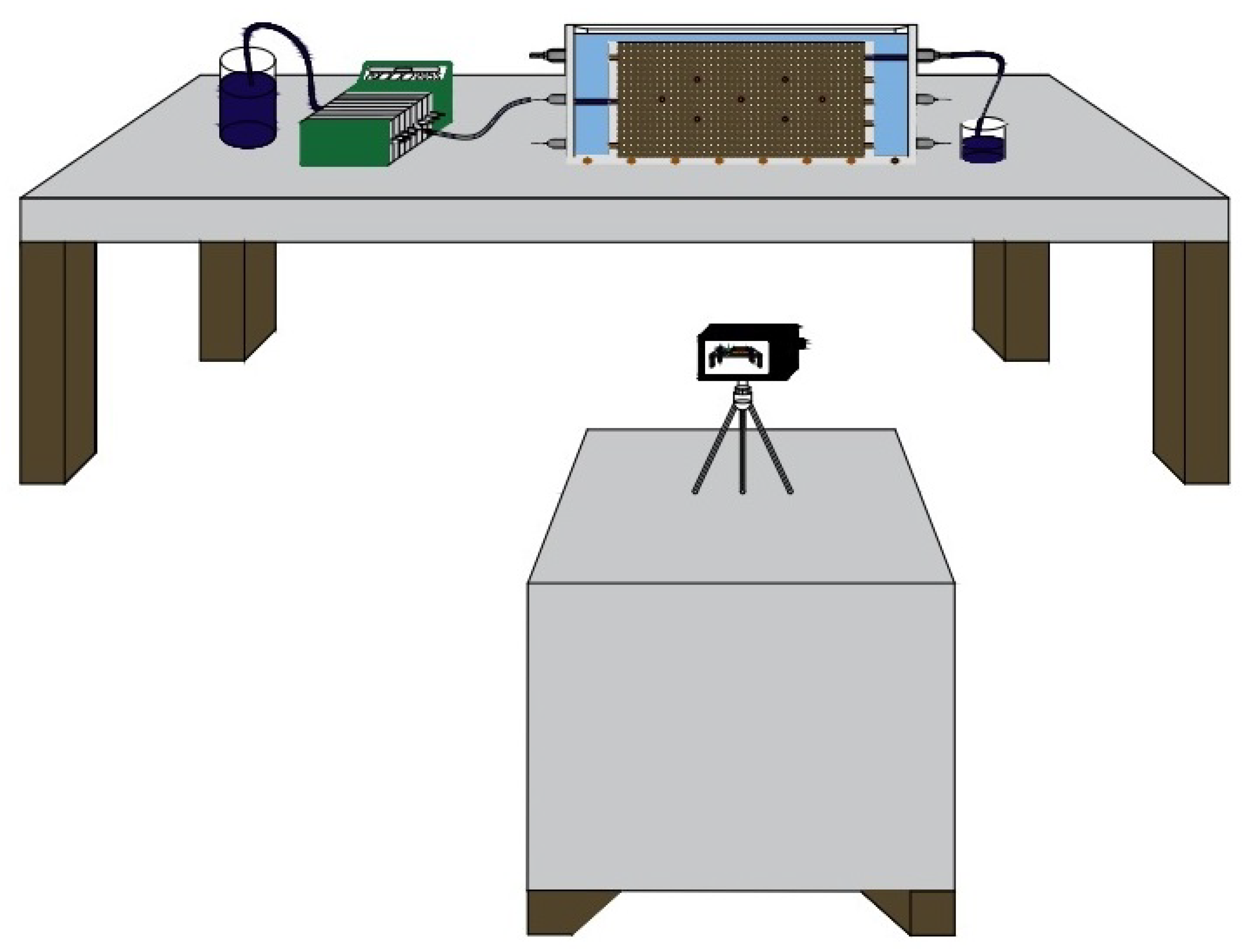
A 0.5% [w/v] potassium permanganate solution was selected and used for the changing plume distribution simulation over time. Because it is a commonly used oxidant for remediation and because of its intense purple color we were able to gain visual observations of the plume’s development. The potassium permanganate was injected into the tank through the end of a 3 mm diameter tube located in the centre of the perforated wall of the tank as illustrated in Figure 2, using specialist tubing that helped control the flow from peristaltic pumps. The injection rate was $16[\mathrm{L}/\mathrm{h}]$. 5.5 liters permanganate were injected from the point source and after completing the injection, the experiment continued until the whole permanganate solution was diluted and washed from the sand by the water flow.

3.3.2. Model Verification with the Analytical Solution

To verify two-dimensional transport problems, the following combined advection-diffusion with the first-order decay rate constant equation is considered as follows

$$\begin{array}{cc}\hfill & {\displaystyle \frac{\partial \mathrm{C}}{\partial \mathrm{t}}}+{\displaystyle \frac{{\rho }_b}{\mathsf{\theta }}}{\displaystyle \frac{\partial \mathrm{S}}{\partial \mathrm{t}}}={\mathrm{D}}_{\mathrm{xx}}{\displaystyle \frac{{\partial }^2\mathrm{C}}{\partial {\mathrm{x}}^2}}-\mathrm{v}{\displaystyle \frac{\partial \mathrm{C}}{\partial \mathrm{x}}}+{\mathrm{D}}_{\mathrm{yy}}{\displaystyle \frac{{\partial }^2\mathrm{C}}{\partial {\mathrm{y}}^2}}-\lambda \mathrm{C},\hfill \\ \hfill & {\displaystyle \frac{\partial \mathrm{S}}{\partial \mathrm{t}}}=\alpha \left({\mathrm{k}}_{\mathrm{d}}\mathrm{C}-\mathrm{S}\right),\hfill \end{array}$$

(19)

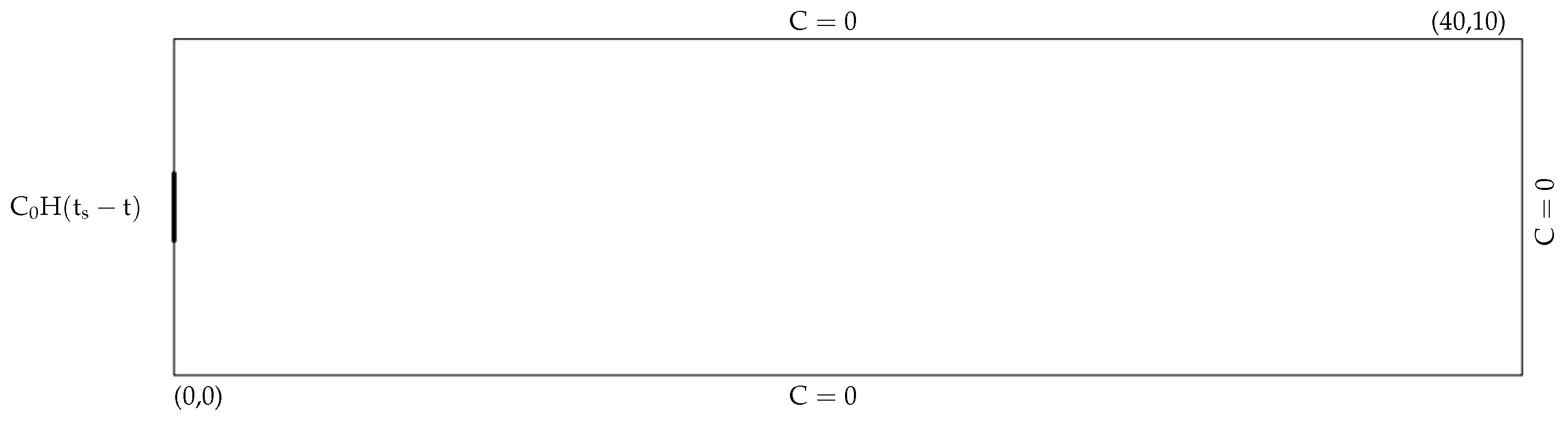
where $\mathrm{C}$ is the contaminant concentration $\left[{\mathrm{ML}}^3\right]$, ${\rho }_b$ is the Bulk density of soil $\left[{\mathrm{ML}}^3\right]$, θ is soil porosity, $\mathrm{S}$ is Sorbed concentration $\left[{\mathrm{MM}}^{-1}\right]$, ${\mathrm{D}}_{\mathrm{xx}}$ and ${\mathrm{D}}_{\mathrm{yy}}$ are diffusion coefficients in $\mathrm{x}$ and $\mathrm{y}$ directions $\left[{\mathrm{L}}^2{\mathrm{T}}^{-1}\right]$, $\lambda$ is the first-order decay rate constant $\left[{\mathrm{T}}^{-1}\right]$, $\alpha$ is the first-order desorption rate constant $\left[{\mathrm{T}}^{-1}\right]$ and ${\mathrm{k}}_{\mathrm{d}}$ is the sorption distribution coefficient and is dimensionless. The initial and boundary conditions c.f. Figure 3 are

$$\begin{array}{cc}\hfill & \mathrm{C}\left(\mathrm{x},\mathrm{y},0\right)=0;\mathrm{S}\left(\mathrm{x},\mathrm{y},0\right)=0\left(\mathrm{x},\mathrm{y}\right)\in \Omega ,\hfill \\ \hfill & \mathrm{C}\left(0,\mathrm{y},\mathrm{t}\right)=\{\begin{array}{l}{\mathrm{C}}_0\mathrm{H}\left({\mathrm{t}}_{\mathrm{s}}-\mathrm{t}\right){\mathrm{y}}_{\mathrm{b}}⩽\mathrm{y}⩽{\mathrm{y}}_{\mathrm{t}}\\ 0\end{array},\hfill \\ \hfill & \mathrm{y}=0,10;0⩽\mathrm{x}⩽40;\mathrm{C}=0,\hfill \\ \hfill & \mathrm{x}=40;0⩽\mathrm{y}⩽10;\mathrm{C}=0.\hfill \end{array}$$

(20)

The analytical solution to this problem in the Laplace domain was given by [44] as follows

$$\begin{array}{c}\hfill {\displaystyle \overline{\mathrm{C}}\left(\mathrm{x},\mathrm{y},\mathrm{s}\right)={\displaystyle \frac{2}{\mathrm{b}}}{\mathrm{C}}_0\left[1-\exp \left(-{\mathrm{t}}_{\mathrm{s}}\mathrm{s}\right)\right]{\displaystyle \sum }_{\mathrm{i}=1}^{\mathrm{N}}\widehat{\overline{\mathrm{C}}}\left(\mathrm{n}\right)\sin \left({\displaystyle \frac{\mathrm{n}\pi \mathrm{y}}{\mathrm{b}}}\right),}\end{array}$$

(21)

where $\mathrm{x}$ and $\mathrm{y}$ are the coordinates in $\mathrm{x}$ and $\mathrm{y}$ directions respectively, $\mathrm{s}$ is the Laplace complex variable, ${\mathrm{C}}_0$ is the concentration at the contaminant source, $\mathrm{b}$ is the aquifer width and $\widehat{\overline{\mathrm{C}}}\left(n\right)$ is presented in Appendix B. The physical constants and parameters for the corresponding analytical solution are are summarized

Table 2. The parameters values for analytical solution.

Parameters	Value
Porosity, θ	25%
Bulk density of soil, ${\rho }_b$	1.5 $\mathrm{kg}/\mathrm{L}$
Diffusion coefficient in $\mathrm{x}$ direction, ${\mathrm{D}}_{\mathrm{xx}}$	0.2 ${\mathrm{m}}^2/\min$
Diffusion coefficient in $\mathrm{y}$ direction, ${\mathrm{D}}_{\mathrm{yy}}$	0.02 ${\mathrm{m}}^2/\min$
velocity, $\mathrm{v}$	1 $\mathrm{m}/{\min }^{-1}$
Contaminant concentration at source	2000 $\mathrm{mg}/\mathrm{L}$
Sorption distribution coefficient, ${\mathrm{k}}_{\mathrm{d}}$	2
First-order decay rate constant, $\lambda$	0.001 ${\mathrm{m}}^2/\min$
First-order desorption rate constant, $\alpha$	1 ${\min }^{-1}$

.

3.4. Remediation Design Optimization Using the GA Approach

A multiobjective optimisation algorithm is applied to the coupled groundwater flow and reactive transport problem considering ISCO remediation by slow release of permanganate. This problem involves finding the set of optimal remediation design regarding the y coordinate of oxidant sources whitin a contaminant plume. The GA is applied to simultaneously maximize the effectiveness of the remediation by minimising the average concentration of the contaminant in the geometry at a shorter time and maximise the region where the contaminant concentration is less than or equal to the final desired concentration of the contaminant and to minimise the cost of the remediation process by decreasing the number of necessary oxidant sources. To achieve this goal, we have defined the following functions:

$$\begin{array}{cc}\hfill & \mathrm{GA}1=\mathrm{t}\mid {\overline{\mathrm{C}}}^1=\zeta {\%}^{\prime }{\overline{\mathrm{C}}}_{\mathrm{initial}}^1\hfill \\ \hfill & \mathrm{GA}2={\Omega }_{{\mathrm{C}}_{\mathrm{FDCC}}^1}=\{\left(\mathrm{x},\mathrm{y}\right)\in \Omega :{\mathrm{C}}^1⩽{\mathrm{C}}_{\mathrm{FDCC}}^1\}\hfill \\ \hfill & \mathrm{GA}3=\mathrm{TC}={\mathrm{n}}_{\mathrm{OS}}\ast \mathrm{COS},\hfill \end{array}$$

(22)

where ${\overline{\mathrm{C}}}^1={\displaystyle \frac{1}{\mathrm{N}}}{{\displaystyle \sum }}_{i=1}^{\mathrm{N}}{\mathrm{C}}^1$ is the average concentration of the contaminant, $\mathrm{N}$ is the number of nodes, ${\mathrm{C}}^1$ is the concentration of the contaminant at each node, ${\mathrm{C}}_{\mathrm{FDCC}}^1$ is the final desired concentration of the contaminant, $\mathrm{TC}$ is the total cost of the remediation process, ${\mathrm{n}}_{\mathrm{OS}}$ is the number of oxidant sources and $\mathrm{COS}$ denotes the cost of each oxidant source. To achieve the objective of the study, we wish to minimise $\mathrm{GA}1$ and $\mathrm{GA}3$ and maximise $\mathrm{GA}2$

$$\begin{array}{cc}\hfill & \min \mathrm{GA}1\hfill \\ \hfill & \max \mathrm{GA}2\hfill \\ \hfill & \min \mathrm{GA}3\hfill \end{array}$$

(23)

by considering the following constraints:

1.

The coordinates of oxidants in the X direction are fixed

$$\begin{array}{c}\hfill {\mathrm{x}|}_{\mathrm{oxidant}\mathrm{sources}}={\mathrm{x}}_{\mathrm{fixed}}\end{array}$$

(24)

2.

The vertical distance between oxidant sources

$$\begin{array}{c}\hfill \mathrm{d}\ge {\mathrm{d}}_{\mathrm{C}},\end{array}$$

(25)

where $\mathrm{d}$ is $|{\mathrm{y}}_{\mathrm{ox}1}-{\mathrm{y}}_{\mathrm{ox}2}|$ and ${\mathrm{d}}_{\mathrm{c}}$ is the critical distance between oxidant sources. The critical distance is the vertical distance between two oxidant sources whose influence domains overlap more than 75%. The influence domain is defined as a region in where the contaminant concentration is less than 85% of its initial concentration after 50 days if it implements alone. The following function defines the influence domain which is used to define critical distance

$$\begin{array}{c}\hfill {\Omega }_{{\mathrm{C}}_{85\%}^1}^{\mathrm{t}=50\mathrm{days}}=\{\left(\mathrm{x},\mathrm{y}\right)\in \Omega :{\mathrm{C}}^1⩽{85\%\mathrm{C}}_0^1\}\end{array}$$

(26)

where ${\mathrm{C}}_0^1$ is initial contaminant concentration.

3.

The number of oxidant sources

$$\begin{array}{c}\hfill {\mathrm{n}}_{\mathrm{OS}}\le 3,\end{array}$$

(27)

where ${\mathrm{n}}_{\mathrm{OS}}$ is the actual number of oxidant sources.

4. Results

4.1. Numerical Model Verification with the Physical Sandbox Model

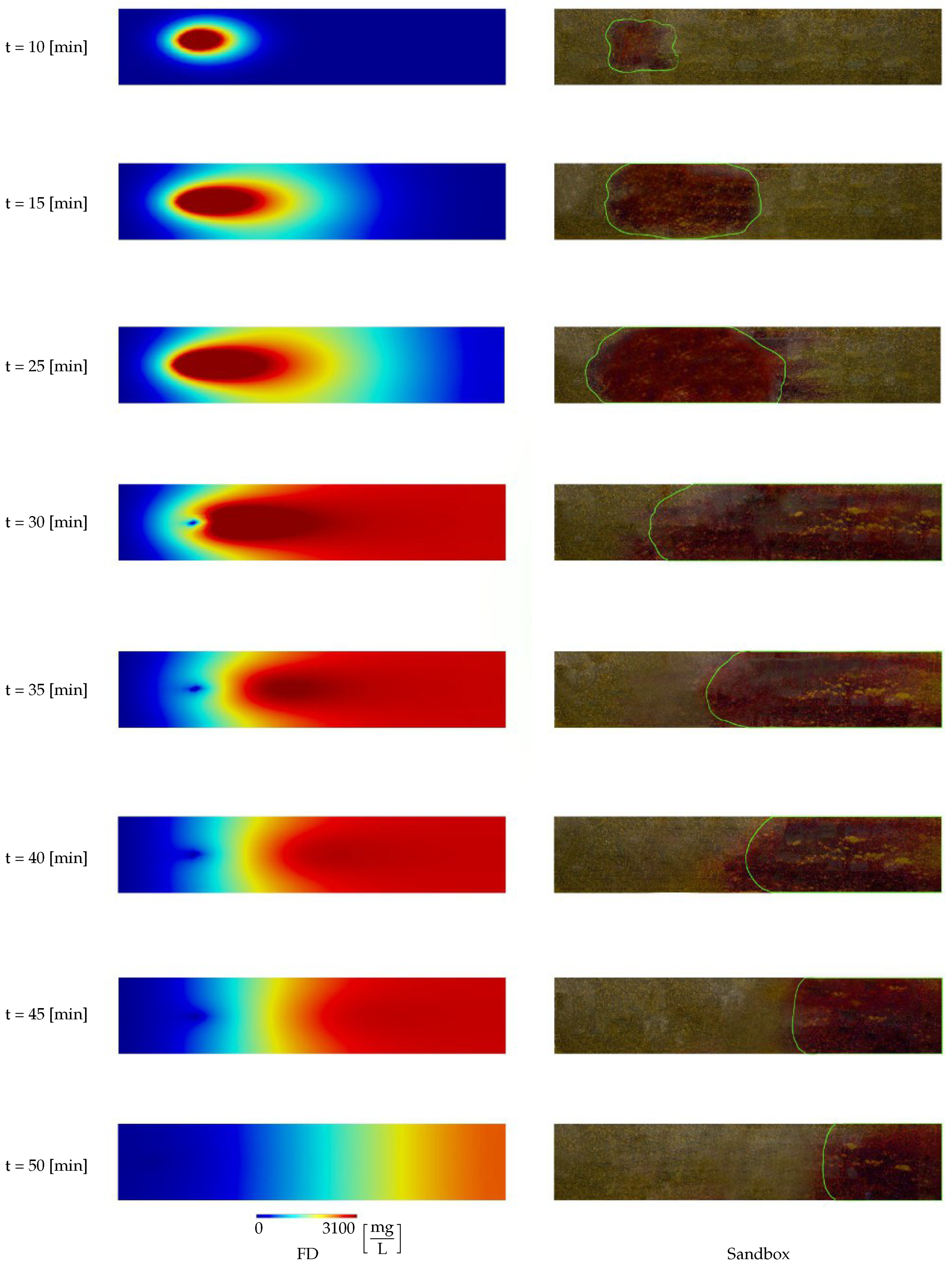
Figure 4 compares the results of the sandbox test and the numerical approach for the different time. To compare the sandbox test and the numerical approach, we have considered three sampling points at the tank, located at $(36,18.5)\left[\mathrm{cm}\right]$, $(56,18.5)\left[\mathrm{cm}\right]$, and $(94,18.5)\left[\mathrm{cm}\right]$ with respect to the origin which is located at the bottom corner of the input end of the tank, and the permanganate concentration was measured every 5 min after the injection. The percentage difference between the measured and predicted concentration shows that the results are in good agreement cf.

Table 3. Comparison of permanganate-measured concentration at sampling points to FD-predicted concentration.

Time	Sample Point	Measured	MFree Predicted	Percentage
[min]	Number	Concentration [mg/L]	Concentration [mg/L]	Difference %
	1	2822	2805	0.61
5	2	2508	2493	0.62
	3	316	312	1.5
	1	3072	3056	0.52
10	2	3110	3092	0.59
	3	320	317	0.93
	1	3052	3041	0.38
15	2	2969	2953	0.55
	3	928	923	0.53
	1	2976	2965	0.36
20	2	2899	2887	0.42
	3	2496	2484	0.48
	1	1057	1071	0.35
25	2	2982	2973	0.31
	3	2758	2751	0.26
	1	388	387	0.38
30	2	1856	1852	0.26
	3	3398	3080	9.30
	1	342	342	0.11
35	2	456	456	0.19
	3	2822	2792	1.07
	1	327	327	0.00
40	2	385	385	0.00
	3	2192	2170	1.07
	1	313	313	0.00
45	2	352	352	0.00
	3	2004	1985	0.97
	1	309	309	0.00
50	2	340	340	0.00
	3	1427	1416	0.78
	1	307	307	0.00
55	2	329	329	0.00
	3	940	934	0.72
	1	300	300	0.00
60	2	314	314	0.00
	3	404	402	0.61

. During the experimental procedure, the concentrations recorded were similar between the different observation points. There was a peak concentration of permanganate in observation point no. 3 after 30 min compared with the other observation points and initial concentrations. This peak occurred by the movement of the mass and the compression in specific points, and the dilution effect caused by the hydrodynamic dispersivity is smaller on this scale than in real conditions.

4.2. Model Verification with the Analytical Solution

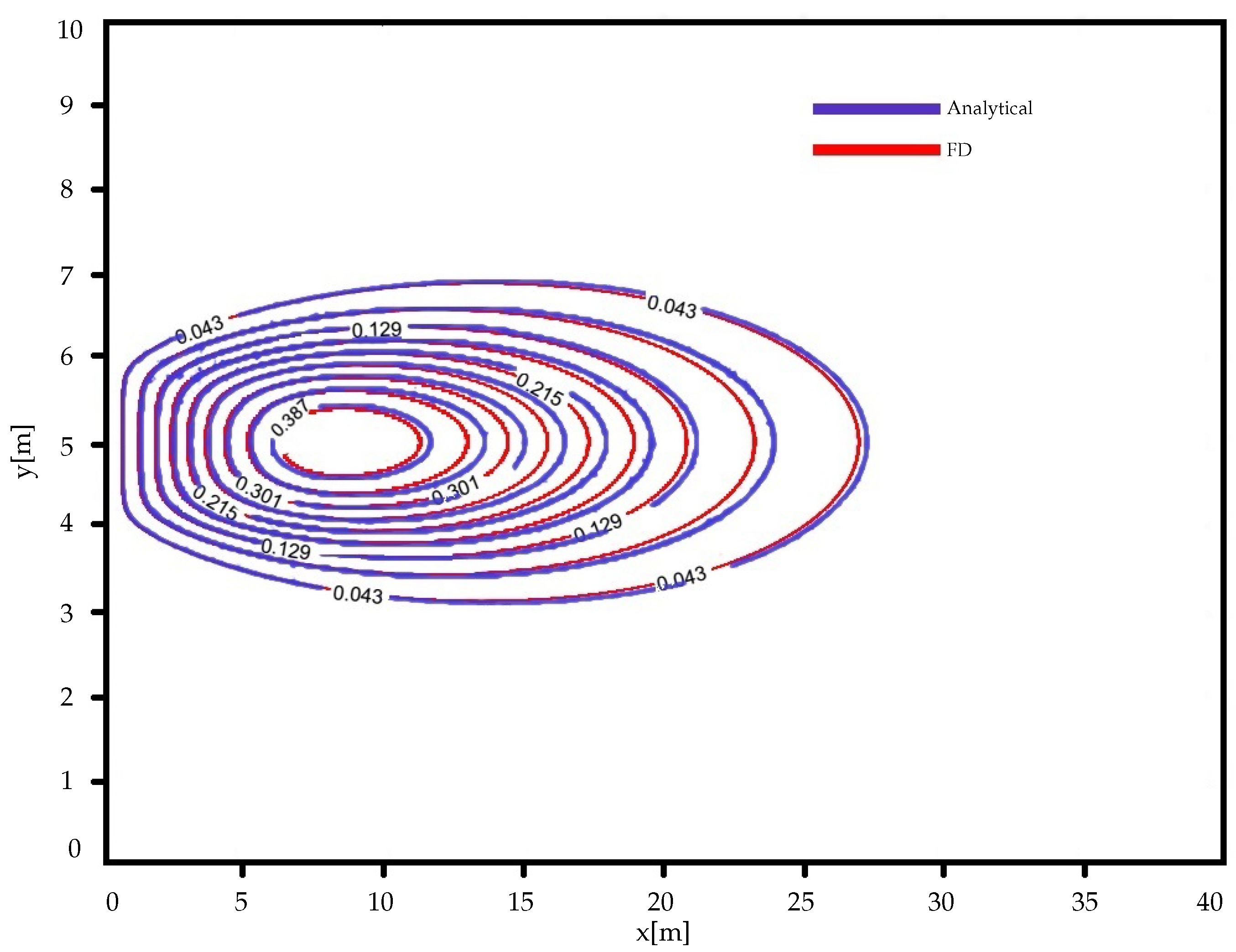
The contaminant of concentration $\mathrm{C}=200\left[\mathrm{mg}/\mathrm{L}\right]$ is injected at $\mathrm{x}=0$$4⩽\mathrm{y}⩽6$, and it requires to find its concentration at the downstream for 100 min. Figure 5 compares the FD and analytical solutions for two-dimensional transport from a continuous line source in a confined aquifer. The simulation was done for t = 100 min.

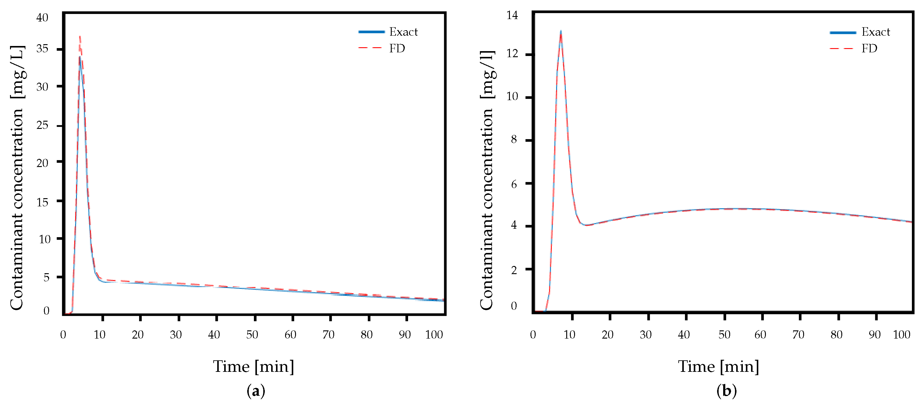
Figure 6a,b the concentration profile at point $\left(5,4\right)$$\mathrm{Pe}=25$ and $\left(9,5\right)$$\mathrm{Pe}=45$. Using analytical solution, we measured the root mean square error (RMSE) as defined below:

$$\begin{array}{c}\hfill {\displaystyle \mathrm{RMSE}=\sqrt{{\displaystyle \frac{{\sum }_{\mathrm{i}=1}^{\mathrm{N}}{\left({\mathrm{c}}_{\mathrm{i}}^{\mathrm{exact}}-{\mathrm{c}}_{\mathrm{i}}^{\mathrm{FD}}\right)}^2}{\mathrm{N}}}}}\end{array}$$

(28)

Table 4. Error measures of the contaminant concentration profile plots of Figure 6.

	RSME
(5,4) (m) Pe = 25	0.743
(9,5) (m) Pe = 45	0.241

shows the RMSE error measures from Figure 6a,b. It can be seen that there is a very good agreement between the FD concentration values and the analytical results.

4.3. Optimized Remediation Design

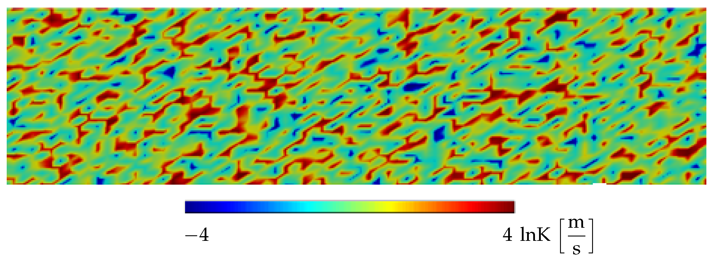
The aquifer domain is made of rectangles of 100 m by 20 m which are heterogeneous regarding hydraulic conductivity. The reliability of groundwater modelling and contaminant transport depends on the quality of the characterisation of hydraulic conductivities. The sequential Gaussian simulation can be used to model conditional stochastic continuous variables such as hydraulic conductivity of an aquifer [45]. The Sequential Gaussian begins with defining the univariate distribution of values, performing a normal score transform of the original values to a standard normal distribution. Figure 7 demonstrates the distribution of hydraulic implemented in the simulation.

We have carried out two different studies, in both of which two oxidant sources have been considered to remediate the contaminant. The second order reaction rate controls the rate of contaminant oxidation by permanganate. The GA approach is used to find the optimum location of oxidant sources with respect to the discussed criteria. The functions presented by [19,46] were modified to simulate the oxidant release.

4.3.1. Study 1

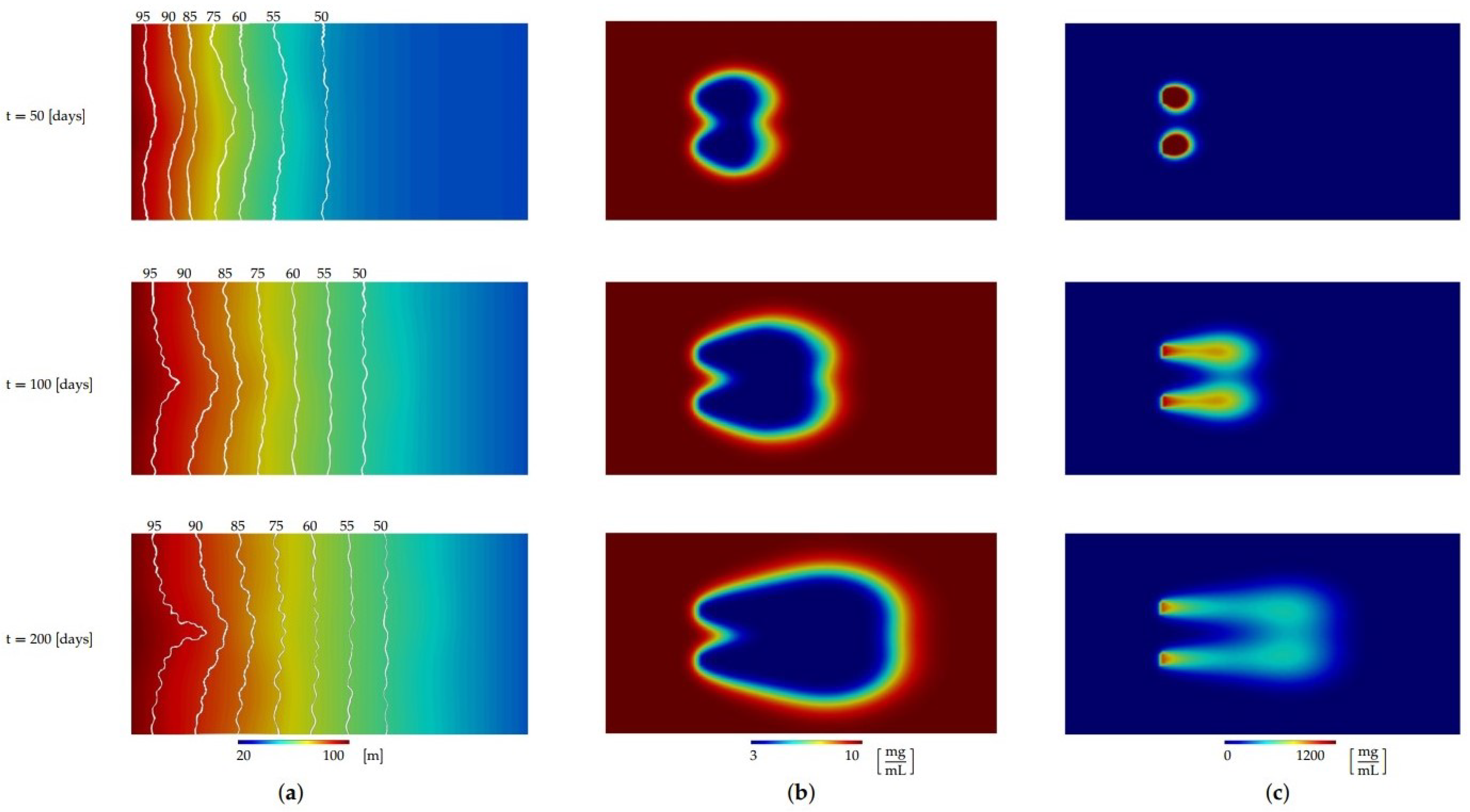
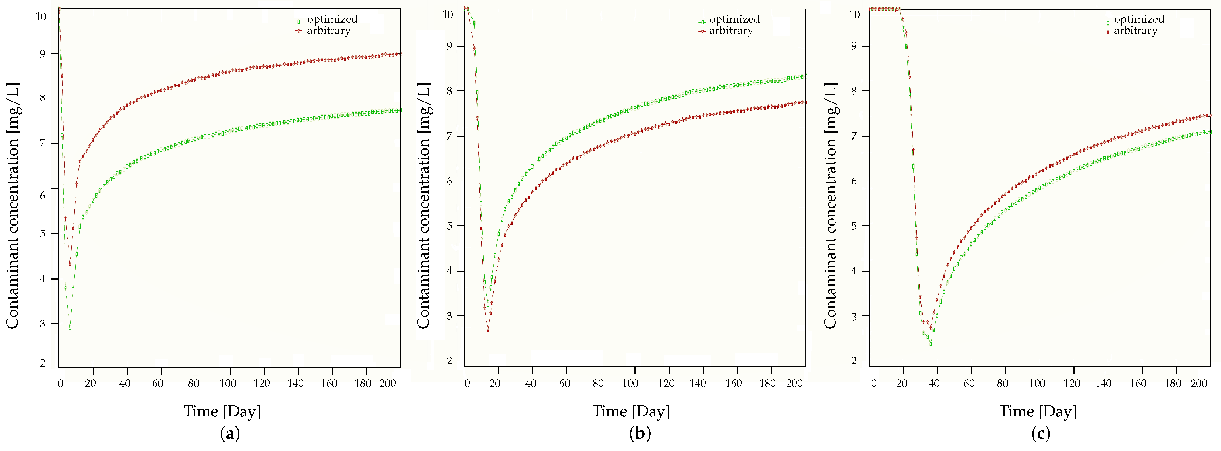
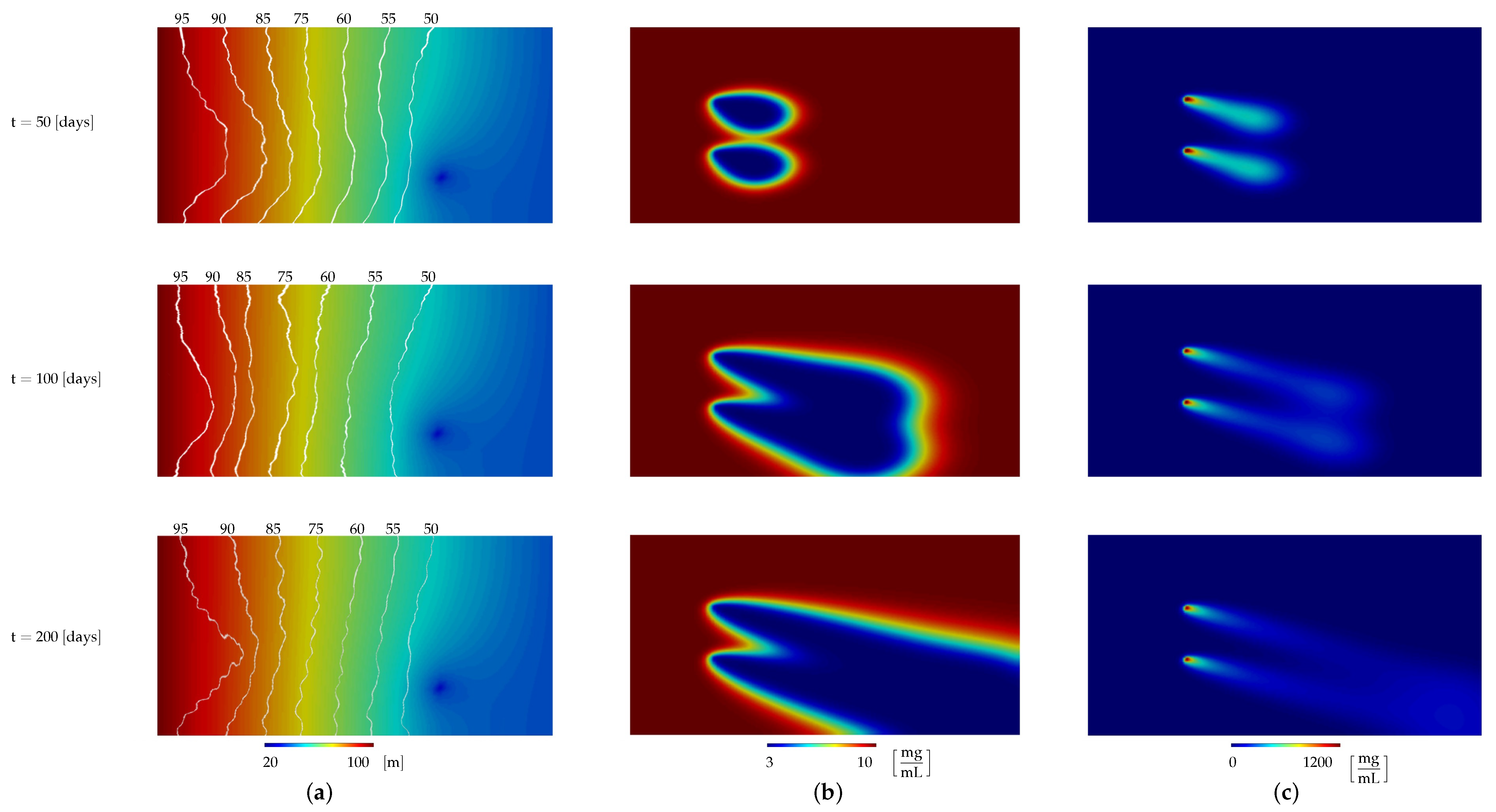
In this study, two oxidant sources have been considered, whose $\mathrm{x}$ coordinates are $\mathrm{x}=20$ m and the optimum y coordinates have resulted from GA. The initial contaminant concentration is ${\mathrm{C}}_{\mathrm{t}0}^1=10[\mathrm{mg}/\mathrm{L}]$ in the whole geometry. Figure 8a demonstrates the iso piezometric head contours. The optimum Y coordinate of the oxidant sources was $7.9\left[\mathrm{m}\right]$ and $12.4\left[\mathrm{m}\right]$. Figure 8b,c show the contaminant and oxidant concentration at different times. The simulations were performed for 200 days and the time step is 0.001 day. Figure 9 illustrates the contaminant concentration at three different observation points located at the (36,10) $\left[\mathrm{m}\right]$, (60,15) $\left[\mathrm{m}\right]$ and (75,10) $\left[\mathrm{m}\right]$ at the downside of the stream. As can be seen in Figure 8a, the piezometric head decreases from left to right overall. Contours of piezometric heads have peaks between the oxidant sources, as expected. As time passes, the piezometric head increases in value and its contours have higher peaks between the oxidant sources. Also, from Figure 8b,c, contaminant and oxidant concentration spreads the middle line of the aquifer symmetrically and skewed towards the right side along the x-direction, as contaminant flows from left to right. Over time, contaminant concentration decrease with the minimum value obtained near the oxidant sources.

4.3.2. Study 2

In the second study a pumping borehole which is located at (75,5) m is considered for piezometric head which causes the contaminant and oxidant to flow to the bottom-left of the geometry. Figure 10a demonstrates the piezometric head considering a pumping borehole, and Figure 10b,c show the contaminant and oxidant concentration at different time steps. The optimum Y coordinate of the oxidant sources was $3.1$ $\left[\mathrm{m}\right]$ and $7.4$ $\left[\mathrm{m}\right]$. The piezometric head decreases overall from the left up corner to the right down corner of the aquifer. Same as study 1, Piezometric head contours, as predicted, have maximum levels between the oxidizing sources. The piezometric head increases in value as time passes, and its contours between oxidant sources have higher peaks. From Figure 10b, it can be easily observed that contaminant concentration decrease with time and contaminant reduces along the water flow direction.

5. Discussion

The purpose of our numerical study is to better understand the remediation process of groundwater through the release of permanganate considering full tensor of hydraulic conductivity which resembles the real condition of the aquifer. To find the critical distance between two sources, we carried out prior simulations to decrease the simulation time. We found that the critical distance in our simulation is ${\mathrm{d}}_{\mathrm{c}}=3.6\left[\mathrm{m}\right]$. The results of prior simulations revealed that if the vertical distance between two sources is less than the critical distance, in some cases the reaching time to the desire average concentration in the geometry is more than implementing only one oxidant source located at $(20,5)\left[\mathrm{m}\right]$, and it can translate as reducing the performance of the remediation design. The effect of considering the full tensor of hydraulic conductivity in the flow equation is evident in the iso-head contours, and it is especially important for contaminant transport predictions because the velocity Equation (8) is affected by this. Overall, the water head contours decreased from left to right, and it mounded between two oxidant sources as expected. As we expected, the concentration of oxidant closer to the sources behave similar to the sources, but with increased distance from sources it changes rapidly. Farther away from sources, e.g. three times more than the distance between oxidant sources, there is less impact on the contaminant concentration. In the first study after 65 days, the contaminant concentration reached the 70% of initial contaminant concentration, while in the second study after 68 days. From Figure 9 it is obvious that the contaminant concentration in optimized remediation design is much less than arbitrary design, which is randomly generated. In Study 1 the maximum difference between contaminant concentration at observation points located at (36,10) m, (60,15) m and (75,10) are 32.8%, 33.7% and 41.2% respectively and it occures at day 7, 14 and 36 after remediation, but after that the difference decreases reaching 14%, 8% and 6.5% at first, second and third observation point respectively. In other words, to reach the same contaminant concentration in the arbitrary design, either initial permanganate concentration at the sources must be higher, or the number of sources has to increase leading to higher cost. It can be concluded that the optimised process improves oxidant concentration and influence farther from the sources early on in treatment, though it has greater impact in the region close to the sources in later stages when compared to arbitrary design.

6. Conclusions

In this study, the simulation-optimisation model of groundwater and reactive transport of contaminant and slow release of permanganate, using the modification of the presented function by [19,46] for our study, in an anisotropic porous aquifer have been developed. The groundwater flow has been simulated considering heterogeneity regarding hydraulic conductivity using its full tensor leading to the simulation resembles a real aquifer. The developed model was verified using the sandbox experiment and analytical solution and has been applied to two different studies. In both studies, the optimum Y coordinates of oxidant sources using GA have been found. To find these optimum locations, three criteria were considered, including minimising the average concentration of contaminant and remediation costs in terms of the number of remediation sources and maximising the influence domain of the oxidant. The results revealed that optimisation reduces not only the time to reach the desired concentration but also the number of oxidant sources necessary, hence reducing the overall remediation cost. In addition, in the beginning of treatment with the optimised design, areas farther from oxidant sources were greater positively with higher oxidant concentrations, later on, however, the regions closer to the oxidant sources were better affected when compared to those treated with the arbitrary design. We will further extend the proposed model to deal with 3D models and will also find the optimum design of oxidant sources in the complex geometries. The next step will be to compare the effectiveness of the FD, FEM and Meshless methods to simulate the reactive transport of solutes in groundwater.

References

- Mondal, P.K.; Furbacher, P.D.; Cui, Z.; Krol, M.M.; Sleep, B.E. Transport of polymer stabilized nano-scale zero-valent iron in porous media. J. Contam. Hydrol. 2017. [Google Scholar] [CrossRef]
- Zhao, Z.; Illman, W.A.; Berg, S.J. On the importance of geological data for hydraulic tomography analysis: Laboratory sandbox study. J. Hydrol. 2016, 542, 156–171. [Google Scholar] [CrossRef]
- Lee, E.S.; Schwartz, F.W. Characteristics and applications of controlled–release KMnO4 for groundwater remediation. Chemosphere 2007, 66, 2058–2066. [Google Scholar] [CrossRef]
- Chen, D.; Carsel, R.; Moeti, L.; Vona, B. Assessment and prediction of contaminant transport and migration at a Florida superfund site. Environ. Monit. Assess. 1999, 57, 291–299. [Google Scholar] [CrossRef]
- Karatzas, G.P.; Pinder, G.F. Groundwater management using numerical simulation and the outer approximation method for global optimization. Water Resour. Res. 1993, 29, 3371–3378. [Google Scholar] [CrossRef]
- Rogers, L.L.; Dowla, F.U. Optimization of groundwater remediation using artificial neural networks with parallel solute transport modeling. Water Resour. Res. 1994, 30, 457–481. [Google Scholar] [CrossRef]
- Molénat, J.; Gascuel-Odoux, C. Modelling flow and nitrate transport in groundwater for the prediction of water travel times and of consequences of land use evolution on water quality. Hydrol. Process. 2002, 16, 479–492. [Google Scholar] [CrossRef]
- Craig, J.R.; Rabideau, A.J. Finite difference modeling of contaminant transport using analytic element flow solutions. Adv. Water Resour. 2006, 29, 1075–1087. [Google Scholar] [CrossRef]
- Robeck, M.; Ricken, T.; Widmann, R. A finite element simulation of biological conversion processes in landfills. Waste Manag. 2011, 31, 663–669. [Google Scholar] [CrossRef]
- Ricken, T.; Sindern, A.; Bluhm, J.; Widmann, R.; Denecke, M.; Gehrke, T.; Schmidt, T.C. Concentration driven phase transitions in multiphase porous media with application to methane oxidation in landfill cover layers. ZAMM J. Appl. Math. Mech. Angew. Math. Mech. 2014, 94, 609–622. [Google Scholar] [CrossRef]
- Traverso, L.; Phillips, T.; Yang, Y. Mixed finite element methods for groundwater flow in heterogeneous aquifers. Comput. Fluids 2013, 88, 60–80. [Google Scholar] [CrossRef]
- Seyedpour, S.M.; Ricken, T. Modeling of contaminant migration in groundwater: A continuum mechanical approach using in the theory of porous media. PAMM 2016, 16, 487–488. [Google Scholar] [CrossRef]
- Xie, Y.; Wu, J.; Nan, T.; Xue, Y.; Xie, C.; Ji, H. Efficient triple-grid multiscale finite element method for 3D groundwater flow simulation in heterogeneous porous media. J. Hydrol. 2017, 546, 503–514. [Google Scholar] [CrossRef]
- Seyedpour, S.; Janmaleki, M.; Henning, C.; Sanati-Nezhad, A.; Ricken, T. Contaminant transport in soil: A comparison of the Theory of Porous Media approach with the microfluidic visualisation. Sci. Total Environ. 2019, 686, 1272–1281. [Google Scholar] [CrossRef]
- Liu, X. Parallel Modeling of Three-dimensional Variably Saturated Ground Water Flows with Unstructured Mesh using Open Source Finite Volume Platform Openfoam. Eng. Appl. Comput. Fluid Mech. 2013, 7, 223–238. [Google Scholar] [CrossRef]
- Guneshwor Singh, L.; Eldho, T.I.; Vinod Kumar, A. Coupled groundwater flow and contaminant transport simulation in a confined aquifer using meshfree radial point collocation method (RPCM). Eng. Anal. Bound. Elem. 2016, 66, 20–33. [Google Scholar] [CrossRef]
- Seyedpour, S.; Kirmizakis, P.; Brennan, P.; Doherty, R.; Ricken, T. Optimal remediation design and simulation of groundwater flow coupled to contaminant transport using genetic algorithm and radial point collocation method (RPCM). Sci. Total Environ. 2019, 669, 389–399. [Google Scholar] [CrossRef]
- Praveen Kumar, R.; Dodagoudar, G.R. Two-dimensional modelling of contaminant transport through saturated porous media using the radial point interpolation method (RPIM). Hydrogeol. J. 2008, 16, 1497. [Google Scholar] [CrossRef]
- Yao, G.; Bliss, K.M.; Crimi, M.; Fowler, K.R.; Clark-Stone, J.; Li, W.; Evans, P.J. Radial basis function simulation of slow-release permanganate for groundwater remediation via oxidation. J. Comput. Appl. Math. 2016, 307, 235–247. [Google Scholar] [CrossRef]
- Hansen, S.K.; Berkowitz, B. Aurora: A non-Fickian (and Fickian) particle tracking package for modeling groundwater contaminant transport with MODFLOW. Environ. Model. Softw. 2020, 134, 104871. [Google Scholar] [CrossRef]
- Pham, H.T.; Rühaak, W.; Schuster, V.; Sass, I. Fully hydro-mechanical coupled Plug-in (SUB+) in FEFLOW for analysis of land subsidence due to groundwater extraction. SoftwareX 2019, 9, 15–19. [Google Scholar] [CrossRef]
- Liu, Y.; Ao, C.; Zeng, W.; Srivastava, A.K.; Gaiser, T.; Wu, J.; Huang, J. Simulating water and salt transport in subsurface pipe drainage systems with HYDRUS-2D. J. Hydrol. 2021, 592, 125823. [Google Scholar] [CrossRef]
- Sassine, L.; Khaska, M.; Ressouche, S.; Simler, R.; Lancelot, J.; Verdoux, P.; La Salle, C.L.G. Coupling geochemical tracers and pesticides to determine recharge origins of a shallow alluvial aquifer: Case study of the Vistrenque hydrogeosystem (SE France). Appl. Geochem. 2015, 56, 11–22. [Google Scholar] [CrossRef]
- BüRger, C.M.; Kollet, S.; Schumacher, J.; BöSel, D. Short note: Introduction of a web service for cloud computing with the integrated hydrologic simulation platform ParFlow. Comput. Geosci. 2012, 48, 334–336. [Google Scholar] [CrossRef]
- Armanyous, A.M.; Ghoraba, S.M.; Rashwan, I.M.H.; Dapaon, M.A. A study on control of contaminant transport through the soil using equal double sheet piles. Ain Shams Eng. J. 2016, 7, 21–29. [Google Scholar] [CrossRef]
- Illman, W.A.; Zhu, J.; Craig, A.J.; Yin, D. Comparison of aquifer characterization approaches through steady state groundwater model validation: A controlled laboratory sandbox study. Water Resour. Res. 2010, 46. [Google Scholar] [CrossRef]
- Ojuri, O.O.; Ola, S.A. Estimation of contaminant transport parameters for a tropical sand in a sand tank model. Int. J. Environ. Sci. Technol. 2010, 7, 385–394. [Google Scholar] [CrossRef]
- Meenal, M.; Eldho, T.I. Simulation–optimization model for groundwater contamination remediation using meshfree point collocation method and particle swarm optimization. Sadhana 2012, 37, 351–369. [Google Scholar] [CrossRef]
- Ouyang, Q.; Lu, W.; Hou, Z.; Zhang, Y.; Li, S.; Luo, J. Chance-constrained multi-objective optimization of groundwater remediation design at DNAPLs-contaminated sites using a multi-algorithm genetically adaptive method. J. Contam. Hydrol. 2017, 200, 15–23. [Google Scholar] [CrossRef]
- Nourani, V.; Mousavi, S.; Dabrowska, D.; Sadikoglu, F. Conjunction of radial basis function interpolator and artificial intelligence models for time-space modeling of contaminant transport in porous media. J. Hydrol. 2017, 548, 569–587. [Google Scholar] [CrossRef]
- Nourani, V.; Mousavi, S.; Sadikoglu, F.; Singh, V.P. Experimental and AI-based numerical modeling of contaminant transport in porous media. J. Contam. Hydrol. 2017, 205, 78–95. [Google Scholar] [CrossRef]
- Vadiati, M.; Asghari-Moghaddam, A.; Nakhaei, M.; Adamowski, J.; Akbarzadeh, A.H. A fuzzy-logic based decision-making approach for identification of groundwater quality based on groundwater quality indices. J. Environ. Manag. 2016, 184, 255–270. [Google Scholar] [CrossRef]
- Sedki, A.; Ouazar, D. Swarm intelligence for groundwater management optimization. J. Hydroinform. 2011, 13, 520–532. [Google Scholar] [CrossRef]
- Pérez, C.J.; Vega-Rodríguez, M.A.; Reder, K.; Flörke, M. A Multi-Objective Artificial Bee Colony-based optimization approach to design water quality monitoring networks in river basins. J. Clean. Prod. 2017, 166, 579–589. [Google Scholar] [CrossRef]
- Katsifarakis, K.L.; Karpouzos, D.K.; Theodossiou, N. Combined use of BEM and genetic algorithms in groundwater flow and mass transport problems. Eng. Anal. Bound. Elem. 1999, 23, 555–565. [Google Scholar] [CrossRef]
- Tian, N.; Sun, J.; Xu, W.; Lai, C.H. An improved quantum-behaved particle swarm optimization with perturbation operator and its application in estimating groundwater contaminant source. Inverse Probl. Sci. Eng. 2011, 19, 181–202. [Google Scholar] [CrossRef]
- Holland, J.H. Adaptation in Natural and Artificial Systems: An Introductory Analysis with Applications to Biology, Control and Artificial Intelligence; MIT Press: Cambridge, MA, USA, 1992; p. 228. [Google Scholar]
- Bear, J. Hydraulics of Groundwater; McGraw-Hill International Book Co.: New York, NY, USA, 1979. [Google Scholar]
- Bear, J. Hydraulics of Groundwater; Dover Publications: New York, NY, USA, 2007. [Google Scholar]
- Freeze, R.; Cherry, J. Groundwater; Prentice-Hall Inc.: Eaglewood Cliffs, NJ, USA, 1979. [Google Scholar]
- Wang, H.; Anderson, M.P. Introduction to Groundwater Modeling: Finite Difference and Finite Element Methods; W.H. Freeman: San Francisco, CA, USA, 1982. [Google Scholar]
- Nijp, J.J.; Metselaar, K.; Limpens, J.; Gooren, H.P.A.; van der Zee, S.E.A.T.M. A modification of the constant-head permeameter to measure saturated hydraulic conductivity of highly permeable media. MethodsX 2017, 4, 134–142. [Google Scholar] [CrossRef]
- Sarki, A.; Mirjat, M.S.; Mahessar, A.A.; Kori, S.M.; Qureshi, A.L. Determination of Saturated Hydraulic Conductivity of Different Soil Texture Materials. J. Agric. Vet. Sci. 2014, 7, 56–62. [Google Scholar]
- Goltz, M.; Huang, J. Analytical Modeling of Solute Transport in Groundwater. In Analytical Modeling of Solute Transport in Groundwater; John Wiley & Sons, Inc.: Hoboken, NJ, USA, 2017; pp. 1–17. [Google Scholar] [CrossRef]
- Li, L.; Zhou, H.; Jaime Gómez-Hernández, J. Steady-state saturated groundwater flow modeling with full tensor conductivities using finite differences. Comput. Geosci. 2010, 36, 1211–1223. [Google Scholar] [CrossRef]
- Wolf, G. Slow Release Permanganate Cylinders for Sustainable in Situ Chemical Oxidation: Development of a Conceptual Design Tool. Master’s Thesis, Clarkson University, Potsdam, NY, USA, 2013. [Google Scholar]
Figure 1.
The aquifer domain and physical setting of the model.
Figure 2.
Schematic representation of sandbox experimental setup.
Figure 3.
The aquifer domain for the analytical solution.
Figure 4.
The comparison between observed and FD predicted plume.
Figure 5.
Comparison of the FD and Analytical solutions for two-dimensional transport.
Figure 6.
Contaminant concentration profile at: (a) (5,4) m Pe = 25, (b) (9,5) m, Pe = 45.
Figure 7.
The hydraulic conductivity distribution.
Figure 8.
(a) piezometric head profile and contours, (b) contaminant concentration profile, (c) oxidant concentration profile.
Figure 9.
Comparison between contaminant concentration at observation points located at: (a) (36,10) m, (b) (60,15) m and (c) (75,10) m optimized and arbitrary location of the oxidant sources.
Figure 10.
(a) Piezometric head profile and contours, (b) contaminant concentration profile, (c) oxidant concentration profile.