
Neural Network Approach to Retrieving Ocean Subsurface Temperatures from Surface Parameters Observed by Satellites


School of Earth and Space Sciences, University of Science and Technology of China, Hefei 230000, China
*
Author to whom correspondence should be addressed.
Water 2021, 13(3), 388; https://doi.org/10.3390/w13030388
Submission received: 22 December 2020
/
Revised: 18 January 2021
/
Accepted: 29 January 2021
/
Published: 2 February 2021
(This article belongs to the Section Oceans and Coastal Zones)
Abstract
:The extraction of physical information about the subsurface ocean from surface information obtained from satellite measurements is both important and challenging. We introduce a back-propagation neural network (BPNN) method to determine the subsurface temperature of the North Pacific Ocean by selecting the optimum input combination of sea surface parameters obtained from satellite measurements. In addition to sea surface height (SSH), sea surface temperature (SST), sea surface salinity (SSS) and sea surface wind (SSW), we also included the sea surface velocity (SSV) as a new component in our study. This allowed us to partially resolve the non-linear subsurface dynamics associated with advection, which improved the estimated results, especially in regions with strong currents. The accuracy of the estimated results was verified with reprocessed observational datasets. Our results show that the BPNN model can accurately estimate the subsurface (upper 1000 m) temperature of the North Pacific Ocean. The corresponding mean square errors were 0.868 and 0.802 using four (SSH, SST, SSS and SSW) and five (SSH, SST, SSS, SSW and SSV) input parameters and the average coefficients of determination were 0.952 and 0.967, respectively. The input of the SSV in addition to the SSH, SST, SSS and SSW therefore has a positive impact on the BPNN model and helps to improve the accuracy of the estimation. This study provides important technical support for retrieving thermal information about the ocean interior from surface satellite remote sensing observations, which will help to expand the scope of satellite measurements of the ocean.
1. Introduction
The datasets provided by satellite remote sensing have promoted ocean research. However, these datasets are mostly confined to the sea surface because it is difficult for electromagnetic radiation to reach the interior of the ocean [1]. Although large-scale in situ observation projects, such as the Argo buoy, have improved deep ocean data mining [2], the existing observational datasets of the subsurface still do not satisfy the needs of research into the internal processes of the oceans [3,4]. We need to obtain more information about the interior of the ocean because most of the important oceanographic phenomena exist below the surface and these phenomena are useful in studying both the characteristics of the ocean and global climate change [5,6,7,8].
In recent decades, most of the additional heat in the Earth’s climate system has entered the oceans [9] and therefore heating of the ocean interior has become an important factor in slowing down global warming [10,11,12,13]. Several studies have shown that the current stagnation in the increase in the sea surface temperature (SST) is reflected in the warming of the upper ocean [14,15,16]. Changes in the ocean system have important impacts on the atmospheric circulation and global climate change [17]. The air–sea interactions caused by the thermal difference between the land and the sea can affect regional and global large-scale circulation systems, leading to disastrous weather and climate events, such as storm surges [18,19,20,21] and super typhoons [22,23,24]. The change in the thermal condition of the oceans has a very close relationship with monsoon activity [25], affecting both the monsoon circulation and precipitation in the monsoon region, and influencing interannual and interdecadal changes in the regional climate [26,27,28]. Model results have also shown that warming of the upper ocean may be associated with some climate events, such as La Niña and the El Niño-Southern Oscillation (ENSO) [7,29]. However, there have been relatively few studies considering the subsurface as a result of the lack of subsurface data. The subsurface temperature is less affected by the air–sea interface than the SST and its interannual variation is more significant. It therefore has a greater role in climate trends, which means that it is important to explore the internal thermal structure of the ocean.
Although the ocean interior cannot be observed directly by satellites, it is possible to estimate subsurface information from sea surface parameters [6]. Statistical methods are commonly used to obtain information about the subsurface or deep ocean from surface satellite remote sensing data [30,31,32]. Fox [33] built one of the earliest systems used to retrieve 3D information about the ocean through multivariate linear regression: the Modular Ocean Data Assimilation System (MODAS). MODAS has been used to retrieve subsurface temperature/salinity fields through similar techniques using datasets from satellite remote sensing [34]. Global 3D temperature, salinity and velocity fields have been reconstructed through a combination of multiple linear regression and the optimum interpolation method using Argo temperature–salinity profiles and satellite remote sensing datasets [35,36]. Empirical orthogonal function (EOF) analysis is another important statistical method based on a mode-extracting approach to project surface information to subsurface fields [3,37,38]. Based on EOF analysis, the multivariate EOF reconstruction (mEOF-R) method was developed to reconstruct 3D fields of the ocean [39,40,41]. This method performed well in recent studies of the Southern Ocean [42,43].
Dynamic approaches such as the surface quasi-geostrophic theory (SQG) method have been developed to reconstruct 3D ocean fields [44,45,46,47]. An effective SQG (eSQG) approach, which takes the potential vorticity into account, was used to retrieve information about the subsurface ocean using surface parameters such as the sea surface height (SSH) and sea surface density (SSD) [48]. The eSQG approach has been widely applied by many researchers [49,50,51,52,53,54,55,56,57]. However, the SQG methods only perform well in the upper ocean (above 500 m) and are based on the assumption that there is a good correlation between the SSH and SSD. To modify this shortcoming, the interior plus surface quasi-geostrophic (isQG) method was proposed [58,59] and has been validated by both numerical and observational methods [60,61]. Yan [62] proposed an SQG-mEOF-R approach combining the advantages of the mEOF and SQG methods to retrieve information about the ocean interior from surface parameters.
With the development of artificial intelligence, technical routes have been proposed that are different from traditional methods. Ali [1] proposed using neural networks to estimate the subsurface thermal structure of the ocean with the SST, SSH, sea surface wind (SSW), net radiation and net heat flux as the input parameters. Based on a self-organizing map (SOM) neural network, Wu [63] used the SSH, SST and sea surface salinity (SSS) to estimate subsurface temperature anomalies and obtained good retrieval results in the depth range 30–700 m. Bao [64] proposed using a generalized regression neural network with the fruit fly optimization algorithm to retrieve the salinity profile of the Pacific Ocean and achieved better results at the halocline than those obtained using a linear methodology. Su [65] used a support vector machine to retrieve the subsurface temperature of the Indian Ocean and a random forest algorithm [66] to retrieve the subsurface temperature of the global ocean using the SSH, SST, SSS and SSW, which proved that the SSS and SSW are helpful in improving the accuracy of the estimation and provided a technical method of measuring the subsurface temperature of the ocean. Su [67] then improved the accuracy of the estimation by using a geographically weighted regression model that took the distribution of the ocean fields into consideration. K-means clustering and feed-forward artificial neural networks were combined to estimate the subsurface temperature and achieve good results down to 1900 m [68]. Valuable research in retrieving the internal characteristics of the ocean have been carried out using sea surface parameters—for example, using neural network approaches to retrieve the temperature–salinity profile [69], combining an empirical mode projection with satellite altimetry to estimate the 3D structure of the Southern Ocean [70] and taking advantage of both convolutional neural networks and long short-term memory networks to reconstruct the 3D ocean temperature [71].
Sea surface datasets from satellite remote sensing are becoming more important in retrieving subsurface parameters. However, the earlier methods generally rely on statistical or dynamic techniques and do not use artificial intelligence algorithms. The machine learning approaches that have been applied still do not make full and efficient use of sea surface parameters. There is still a need to improve the accuracy of these methods and the retrieval results based on sea surface parameters. Back-propagation neural networks (BPNNs) have been proved to be an extraordinarily useful method in data classification and regression [72,73,74]. We propose a BPNN model to retrieve ocean subsurface temperatures using the SST, SSH, SSS, SSW and sea surface velocity (SSV). The use of the SSV as a non-linear advection term has not been reported previously. The accuracy of our results was evaluated by comparing the estimated temperature field with the reprocessed observational temperature field.
The remainder of this paper is organized as follows. Section 2 introduces the datasets for the study area and the BPNN model. Section 3 evaluates the performance of the BPNN model in estimating the subsurface temperature fields and compares the results estimated by the BPNN model with four and five input parameters. Section 4 presents a short discussion. Our conclusions are presented in Section 5.
2. Study Area, Datasets and Methods
Research on the North Pacific Ocean (NPO) has increased in recent years, with an increasing emphasis on air–sea interactions at mid-latitudes. The NPO is very sensitive to global climate change and has a significant impact on the weather and ecological environment of the neighboring regions of East Asia and North America [75,76,77]. Water temperature is the most important indicator of the thermal state of the ocean and fluctuations will lead to changes in the ocean–atmospheric circulation, which, in turn, affects the Earth’s climate [78,79,80]. It is therefore worth studying the NPO region, especially its thermal structure. The study area of the NPO considered here is located at (0.125–69.875° N, 110.125° E–99.875° W).
We used datasets for the SSH, 3D temperature (3DT), SSS, SSV and SSW. The SSH, 3DT, SSS and SSV data were obtained from the Copernicus Marine and Environmental Monitoring Service (CMEMS; https://marine.copernicus.eu/). Among these, the 3DT is a level 4 gridded reprocessed dataset obtained by combining Argo and satellite remote sensing data [3,34]. Errors on temperature are about 0.8 °C at 100 m and 0.2 °C at 1000 m. The SSH and SSV data were provided by AVISO altimetry (AVISO, http://www.aviso.altimetry.fr/), which is estimated by optimal interpolation, merging the measurements from different altimeter missions (Jason-3, Sentinel-3A, HY-2A, Saral/AltiKa, Cryosat-2, Jason-2, Jason-1, T/P, ENVISAT, GFO, ERS1/2); the data can be downloaded from CMEMS. The errors of SSH have been estimated to be lower than 0.5 mm/year at global scale, and lower than 3 mm/year at regional scale. Errors on SSV have been estimated to range between 10 and 16 cm/s depending on the ocean surface variability. The SSS data were obtained from level 4 re-analyzed datasets through multi-dimensional interpolation of the Soil Moisture and Ocean Salinity (SMOS) product SSS with surface temperature and in situ salinity data [81]. RMS differences of SSS are about 0.1 psu. The 3DT dataset contains 17 depth levels and we used the depth range 0–1000 m. The first depth level (0 m) of the 3DT dataset is the SST. The other 16 depth levels (30, 50, 75, 100, 125, 150, 200, 250, 300, 400, 500, 600, 700, 800, 90 and 1000 m) are used as labels for the training, testing and evaluation of the accuracy of the BPNN model and are referred to here as the observed temperatures. The SSW was provided by the Cross-Calibrated Multi-Platform (CCMP; https://rda.ucar.edu/datasets/ds745.1/) wind velocity product, which combines multisource surface wind data using a variational analysis method to produce high-resolution gridded analyses. To avoid differences between individual years and days, all the datasets used in this study were monthly mean values covering the same time period from January 2005 to December 2015 at a spatial resolution of (0.25° × 0.25°) and covering the same region of the NPO.
Back-propagation is one of the most important and commonly used supervised deep learning algorithms for artificial neural networks [82]. According to the Kolomogorov–Arnold-Sprecher theorem, a three-layer (input-hidden-output) neural network can be used to perform any continuous function [83,84], although both the operational efficiency and the accuracy of the results should be taken into consideration when deciding the number of neurons in the hidden layers [85]. After testing, we decided to use a single hidden layer neural network composed of 15 hidden layer units, for which the input layer obtained the surface features and the output layer gave the predicted temperature field at each depth. The back-propagation algorithm was used for model training.
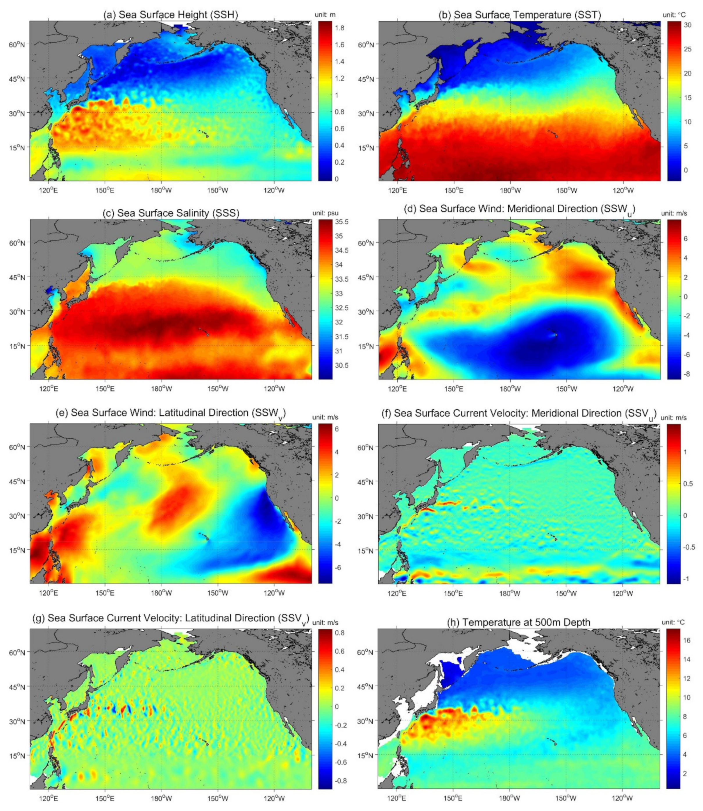
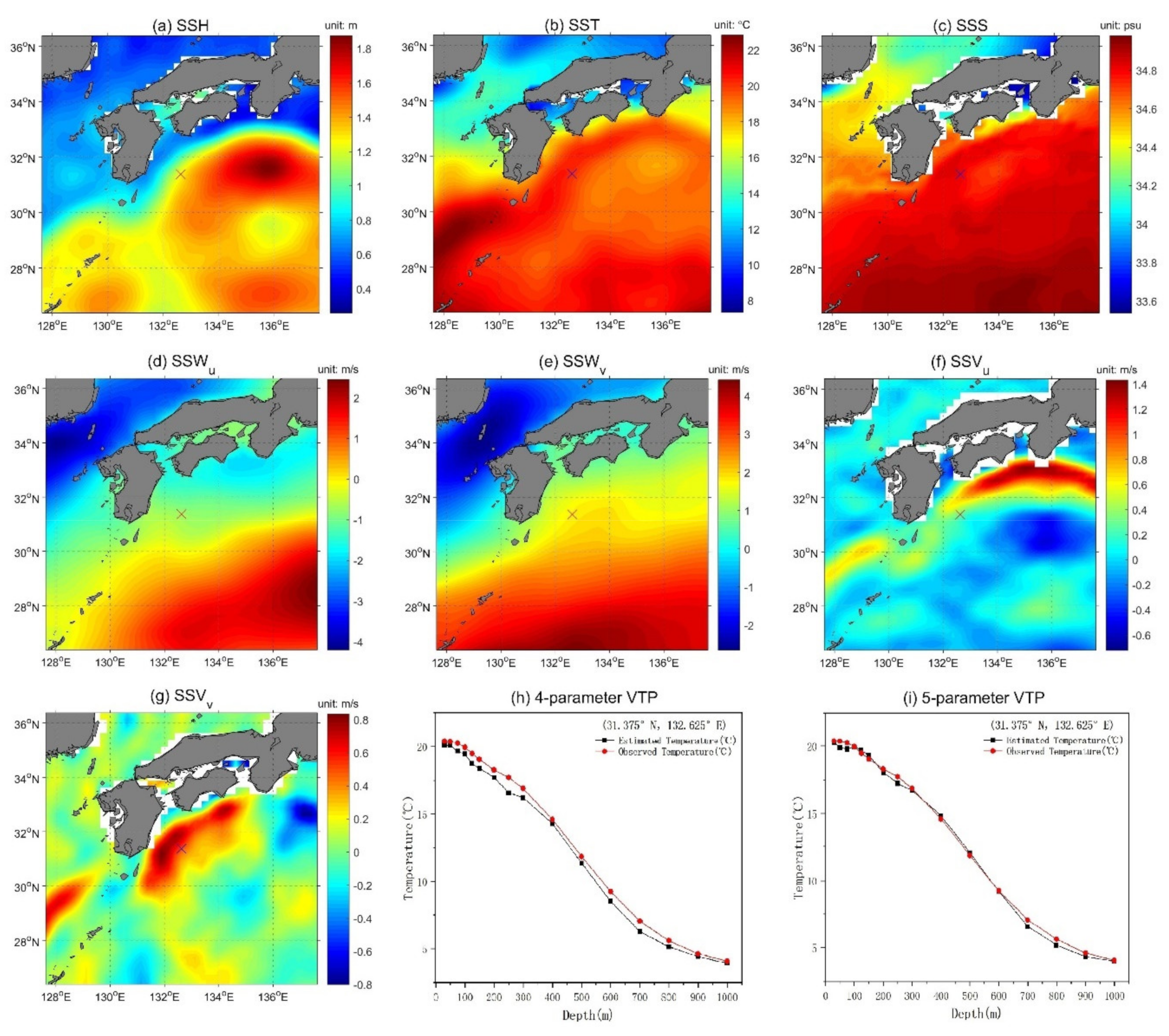
We used the SSH, SST, SSS, SSW and SSV in the NPO as the input or independent parameters for the BPNN model and the output or dependent parameters were the temperature at 16 depth levels. As vectors, the SSW and SSV are divided into two components: (SSWu, SSWv) and (SSVu, SSVv), where the subscripts u and v represent the meridional (positive for northward and negative for southward) and latitudinal (positive for eastward and negative for westward) components, respectively. Figure 1 shows the sea surface parameters (SSH, SST, SSS, SSW and SSV) and the subsurface temperature field (e.g., 500 m depth in March 2015) for the study area. These parameters have their own characteristic spatial distribution. The SSH presents a significant block pattern distribution over the NPO, with an especially high-value area in the southwestern NPO and a low-value area in the northern NPO (Figure 1a). The SST shows a clear zonal distribution in which the temperature decreases significantly as the latitude increases (Figure 1b). In general, the SSS has the highest value around the middle of the NPO and along the equator (Figure 1c). The components of the SSW and SSV show that their spatial distributions are very different. The SSW shows a wide range of regional characteristics, whereas the SSV presents an alternating distribution over the NPO (Figure 1d,e,f,g).
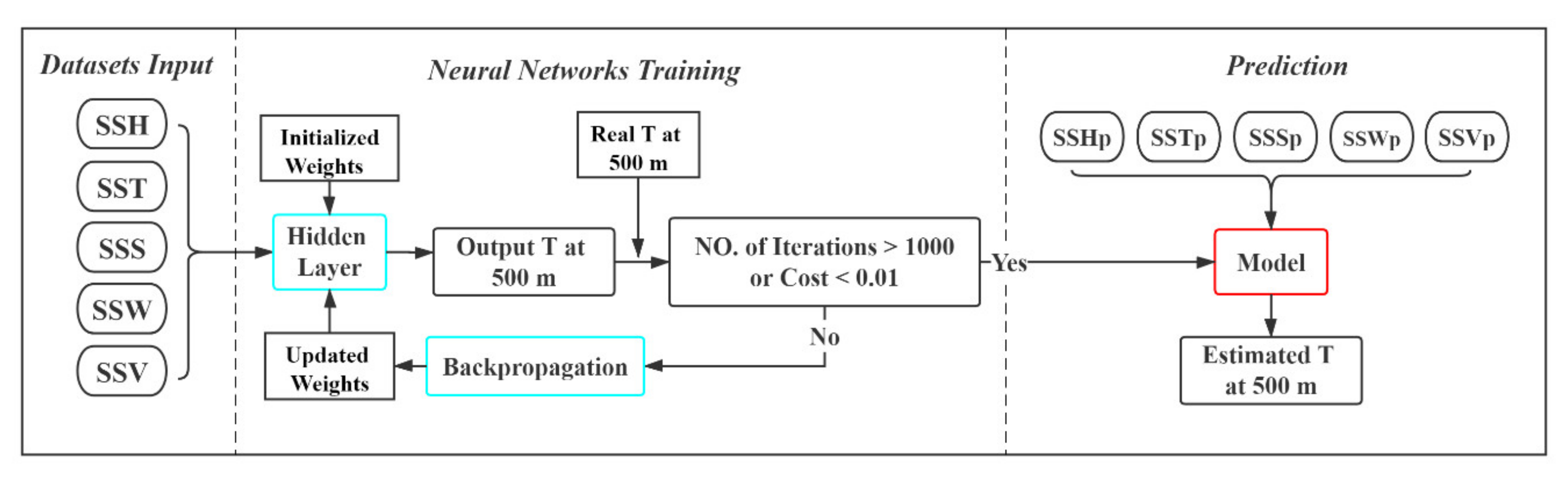
Considering that each depth level has its own unique physical state, the links between its temperature field and the surface parameters should be unique. Therefore, we need to train the subsurface temperature estimation model of each depth level separately. In other words, for each depth level, we will have a corresponding temperature estimation model, which means there will be 16 different models in total because we have 16 different depth levels. Specifically, Figure 2 shows the flow chart for our subsurface temperature estimation algorithm. First, we randomly divided the datasets for the 120 months from January 2005 to December 2014 into two groups: one group used 60% of the data as the training set and the other group used 40% of the data as the validation set. This proportional distribution is reasonable because it is based on a comprehensive consideration of our large dataset and previous research experience [1,63,65,66,67,68,86,87]. The training set was used to train the BPNN model and the validation set was used to validate the model during the training period to prevent overfitting and to optimize the weight values to enhance the prediction ability of the model. We then took the observed temperature at each depth level as the label (or target) and used the back-propagation algorithm for training. The neural networks stopped training and stored the trained weights of the model when the number of iterations reached 1000 or when the mean square error (MSE) between the predicted and observed results was <0.01 °C. The trained BPNN model was then used to predict the output of the test set (the dataset for the 12 months of 2015) at the corresponding depth layers.
The MSE is the average squared difference between the output temperature and the target temperature and is mainly used to evaluate the performance of the BPNN model for different combinations of input parameters at the same depth level. The coefficient of determination (R²) is the proportion of the variance in the dependent variable that is predictable from the independent variables. R² can be used to represent the correlation between the estimated and observed temperature field and to evaluate the performance of the model at different depth levels, in addition to evaluating the performance of the model under different combinations of parameter inputs. A lower MSE and a higher R² represent a better performance of the BPNN model.
3. Results
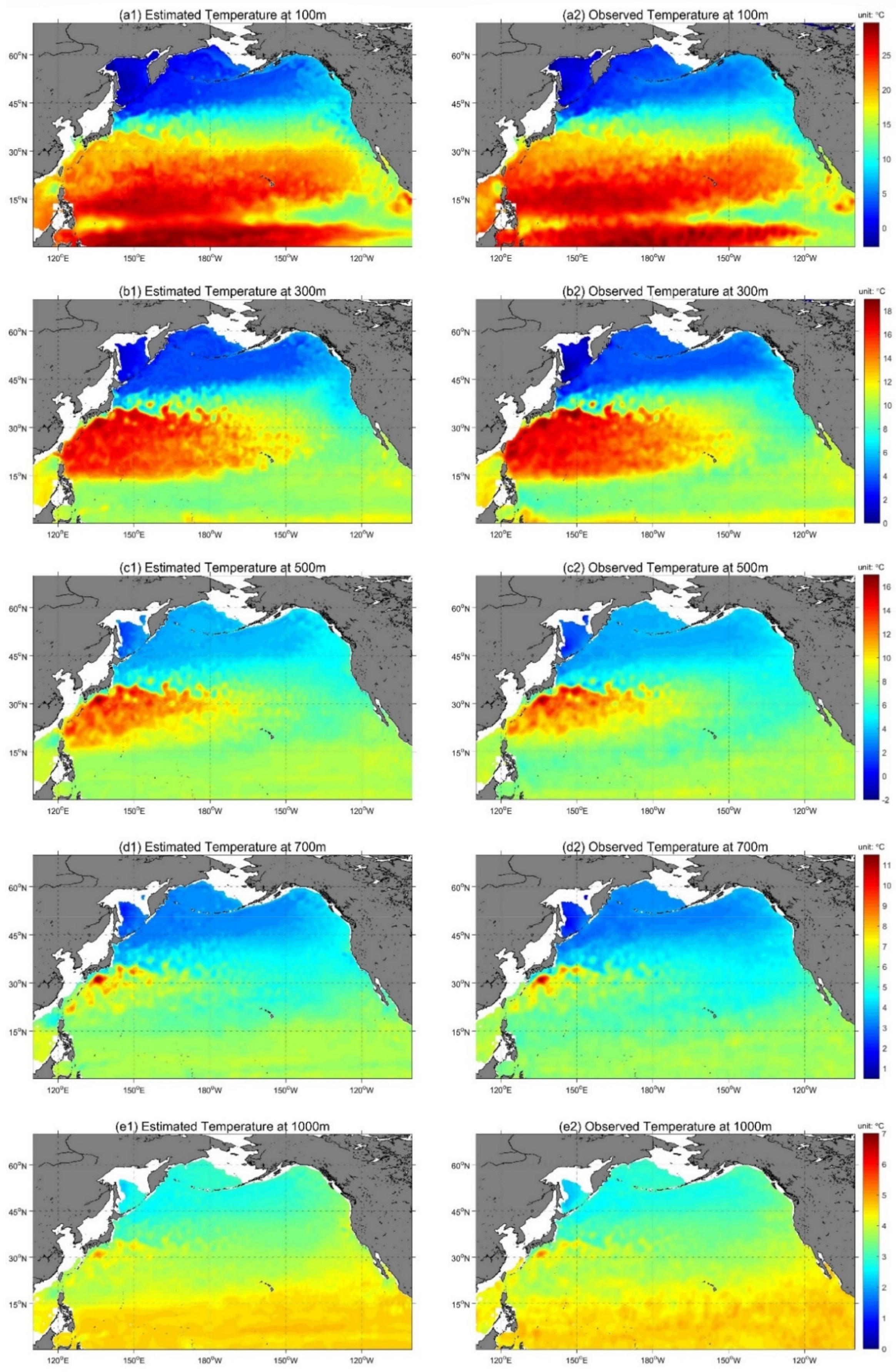
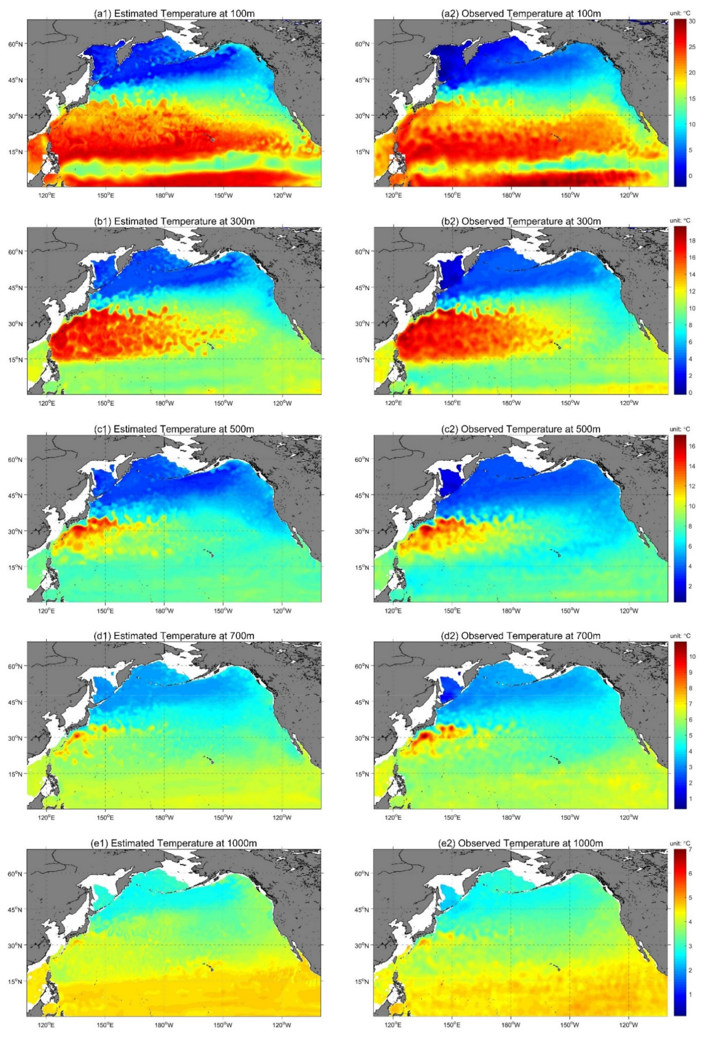
The BPNN model was set up to retrieve the temperature at 16 different depth levels (30, 50, 75, 100, 125, 150, 200, 250, 300, 400, 500, 600, 700, 800, 900 and 1000 m) using the sea surface parameters. Figure 3 and Figure 4 show the temperature fields estimated by the BPNN model with all five input parameters in January and July 2015 (at five different depths of 100, 300, 500, 700 and 1000 m) and the observed temperature field at the same depth for comparison. The temperature field estimated by the BPNN model and the observed temperature field both show a consistent spatial distribution in January 2015 (Figure 3). The temperature field at 100 m depth in the study area shows a zonal distribution and the two high value areas near 15° N and the equator are predicted well by the model (Figure 3a). By contrast, the results for July 2015 (Figure 4) show that the estimated results at 100 m depth are not as good as the estimates in January 2015, which may be related to the active dynamics of the summer NPO decreasing the accuracy of the model estimation in the upper ocean. However, the model accurately predicts the low-temperature zone along 7° N (Figure 4a). The performance of the model at 300–1000 m depth is similar in both January and July, but the spatial distribution of the temperature field is very different from that at 100 m depth and the spatial heterogeneity becomes inconspicuous with increasing depth (Figure 3 and Figure 4), which is related to the relatively stable thermal environment of the deeper ocean. Figure 3 and Figure 4 show the performance of the BPNN model in retrieving the internal temperature field of the NPO. Although the estimations in different months and at different depth levels show regional differences, the model is intuitively satisfactory overall.
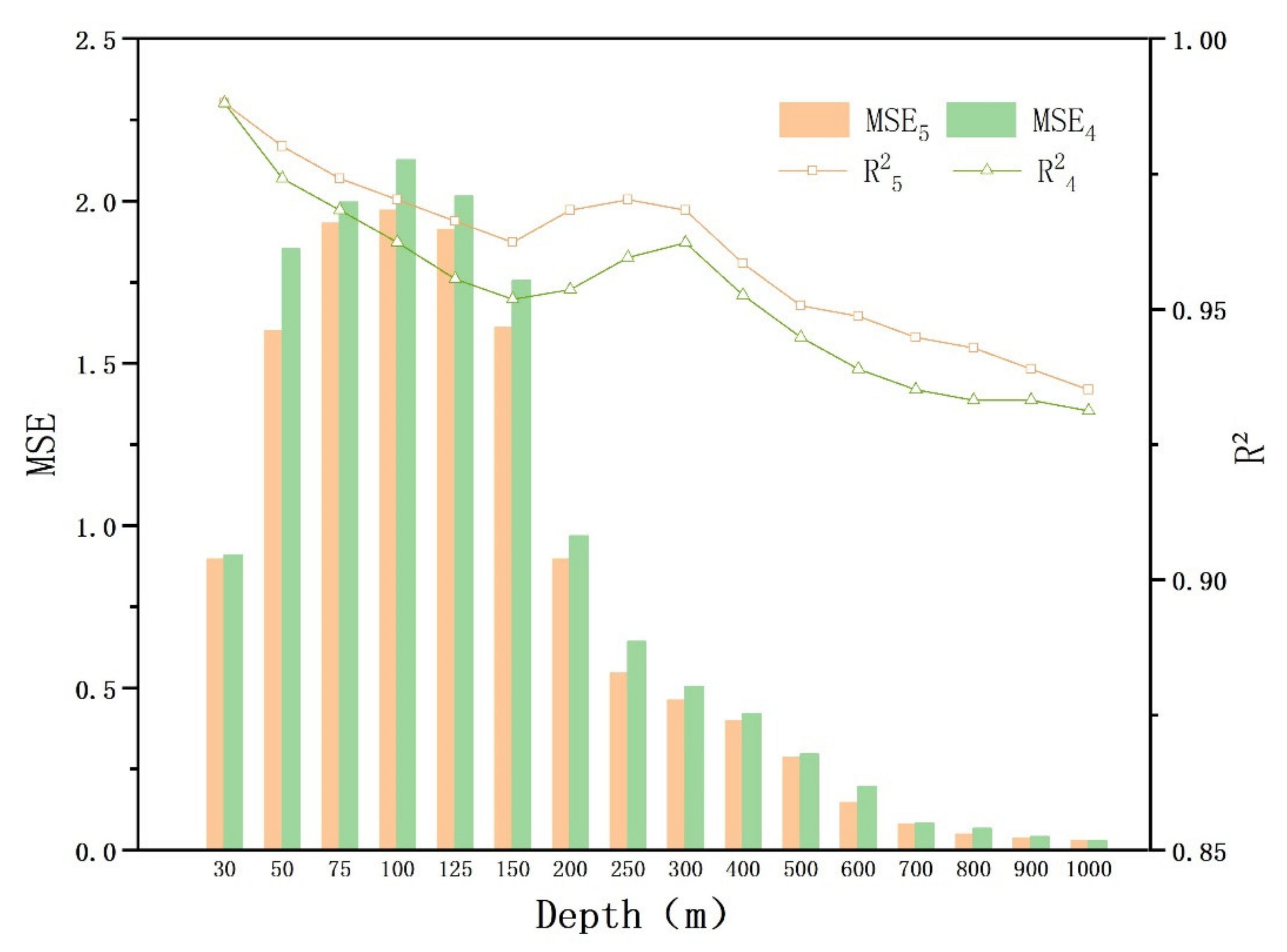
Table 1 and Figure 5 quantify the accuracy of the estimation by the BPNN model using the MSE and R². Taking the five-parameter BPNN model as an example, the corresponding values of the MSE and R² are: MSE = 1.97, R² = 0.970 at 100 m; MSE = 0.462, R² = 0.968 at 300 m; MSE = 0.284, R² = 0.951 at 500 m; MSE = 0.079, R² = 0.945 at 700 m; and MSE = 0.028, R² = 0.935 at 1000 m. This means that the accuracy of the estimation by the BPNN model is different at different depths. Table 1 and Figure 5 show that the MSE values between 50 and 200 m are much higher than the values at other depths, with R² decreasing rapidly from 0.988 (30 m) to 0.962 (150 m). This suggests that the lower accuracy of the estimation by the BPNN model might be related to the complex dynamic processes in the upper ocean and the disturbance of the mixed layer and thermocline. Figure 5 shows that R² gradually decreases from 0.970 (250 m) to 0.935 (1000 m) as the depth increases, which reflects a decrease in the accuracy of the estimation by the BPNN model with increasing depth. This is a result of the difficulty in characterizing the physical state at depth in the ocean relative to the surface as the depth increases. The slow decrease in the MSE at depths >200 m is mainly because the absolute value of the temperature in the deep ocean decreases with depth. The low MSE (0.028–1.970, mean 0.802) and the high R² (0.935–0.988, mean 0.960) quantitatively show that the BPNN model provides a satisfactory estimate of the temperature field of the upper (<1000 m) NPO. It is worth mentioning that CMEMS provided 18 depth levels of subsurface temperature data within the upper 1000 m depth. Besides the 16 depth levels we have used, there are two more depth levels (10 m and 20 m) which have not been discussed in the paper. We have calculated the results of these two depth levels based on five sea surface parameters. The values are MSE = 0.167 and R² = 0.998 at 10 m and MSE = 0.461 and R² = 0.995 at 20 m. We did not use these two depth levels mainly for two reasons: first, the results of 30, 50, 75 and 100 m have showed the model’s performance trend in the upper 100 m, so adding results of 10 m and 20 m will not be necessary. Second, putting them into figures like Figure 5 and Figure 7 will make the points of the upper layers too crowded.
Previous studies have shown that the SSH, SST, SSS and SSW can help to retrieve the subsurface thermal structure [1,65,66,67]. We therefore set up two groups of experiments with different input parameter combinations to determine how the SSV affects the performance of the model output. The BPNN input parameters in the first group were the SSH, SST, SSS and SSW. The BPNN input parameters in the second group were the SSH, SST, SSS, SSW and SSV. The results (Table 1) show that the performance of the model not only varies at different depths, but also varies between different combinations of input parameters. For all 16 depths, the mean MSE of the five- and four-parameter BPNN model are 0.802 and 0.868, respectively, with mean R² values of 0.960 and 0.952, respectively. On average, the five-parameter BPNN model performs better than the four-parameter model as a result of its lower mean MSE and higher mean R². Figure 5 shows that the five-parameter BPNN model has a significantly lower MSE and higher R² than the four-parameter BPNN model at every depth, which further proves that the SSV can improve the accuracy of the estimation of the BPNN model in the NPO. These results further prove that SSV may play an important part in connecting the surface and internal ocean through ocean processes such as non-linear advection dynamics.
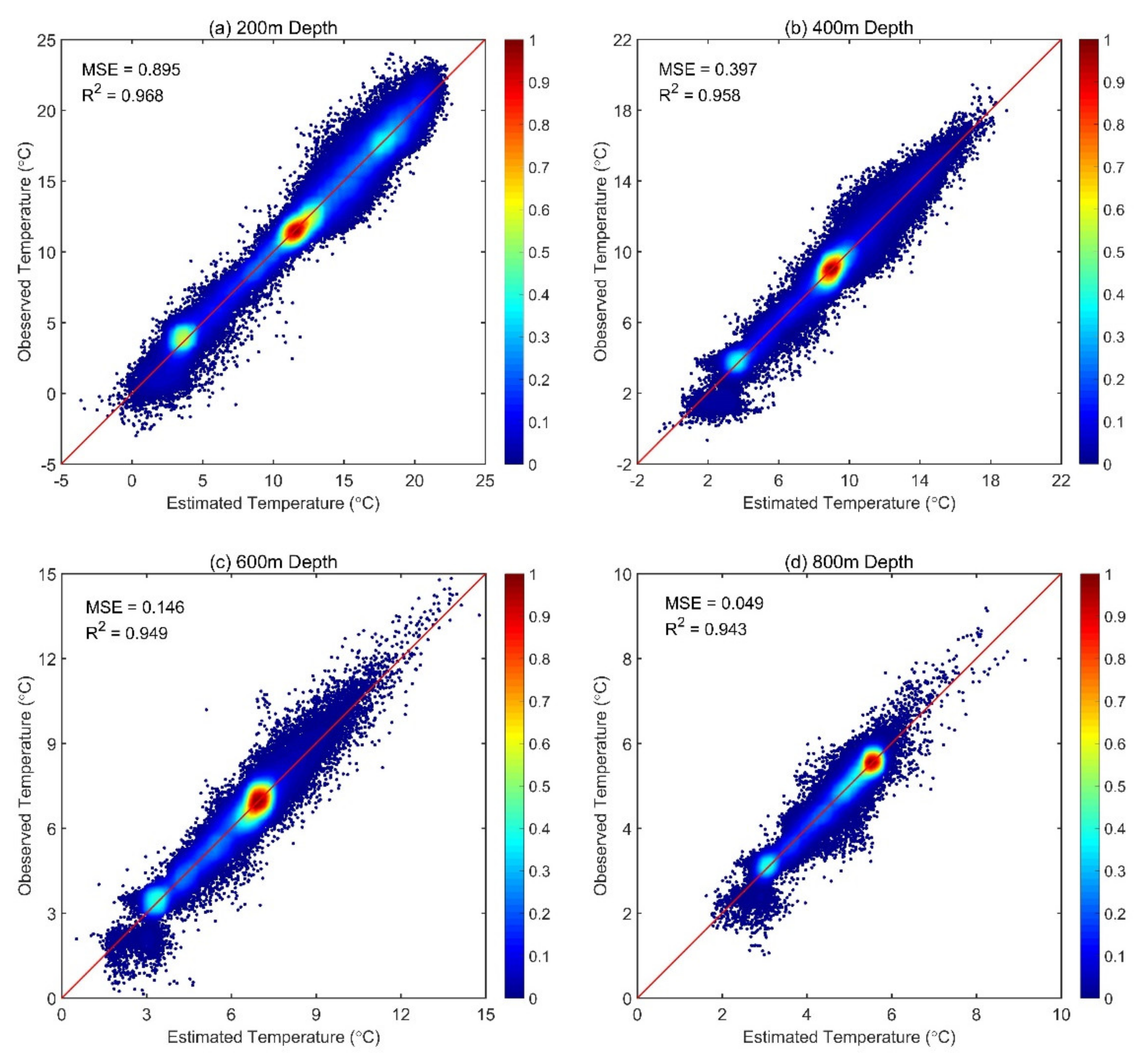
We used density scatter plots (Figure 6) to show the relationship between the temperature estimated by the five-parameter BPNN model and the observed temperature at 200 m (MSE = 0.895, R² = 0.968), 400 m (MSE = 0.397, R² = 0.958), 600 m (MSE = 0.146, R² = 0.949) and 800 m (MSE = 0.049, R² = 0.943). The accuracy of the estimation by the model can be tested directly by scatter regression and the temperature estimated by the BPNN model was verified by the observed temperature, which showed a low MSE and high R² (Figure 6). Figure 6 shows that most of the points are distributed evenly and densely along the isoline, indicating that the estimated results from the BPNN model are reliable and the model performs well in the study area.
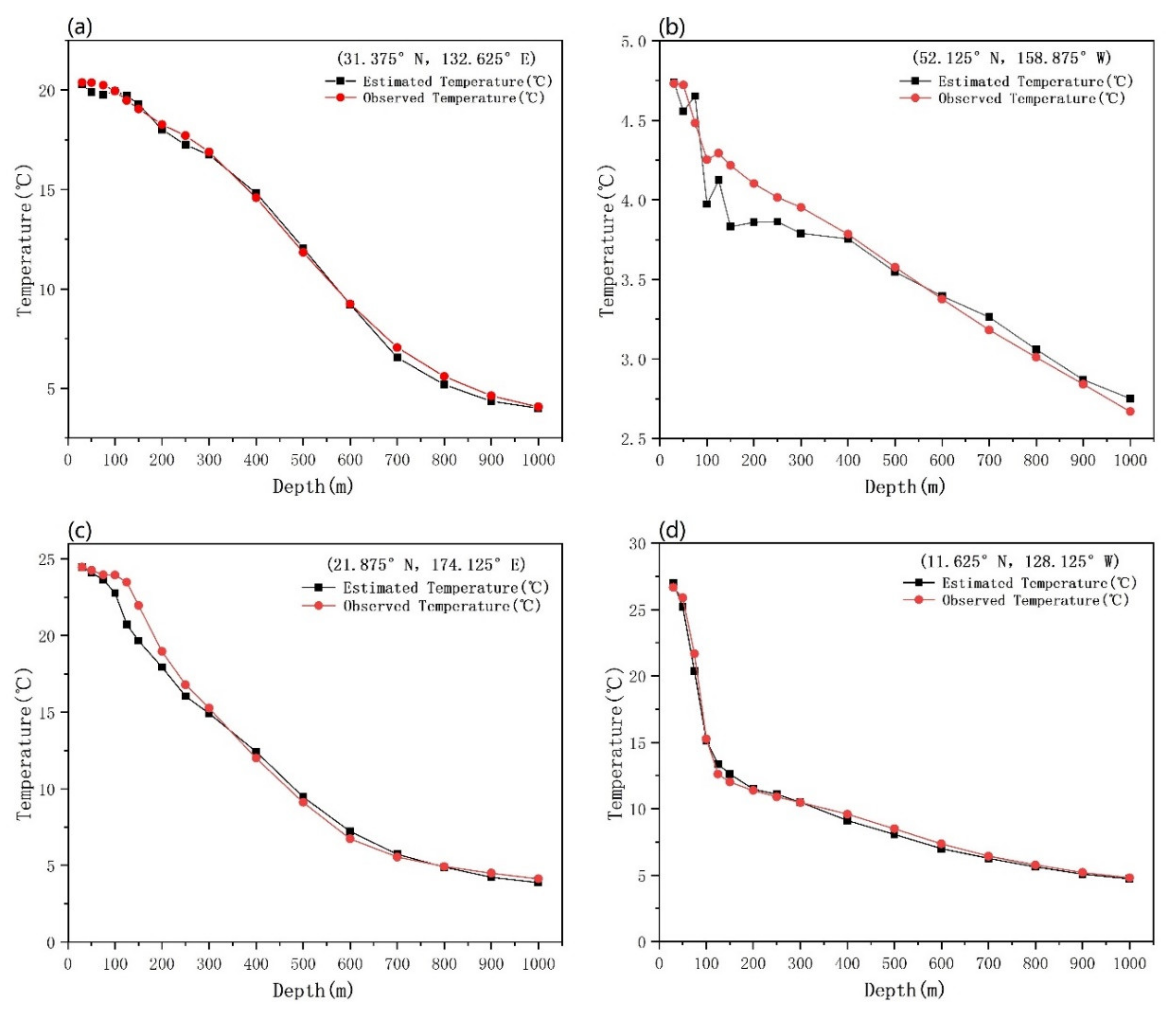
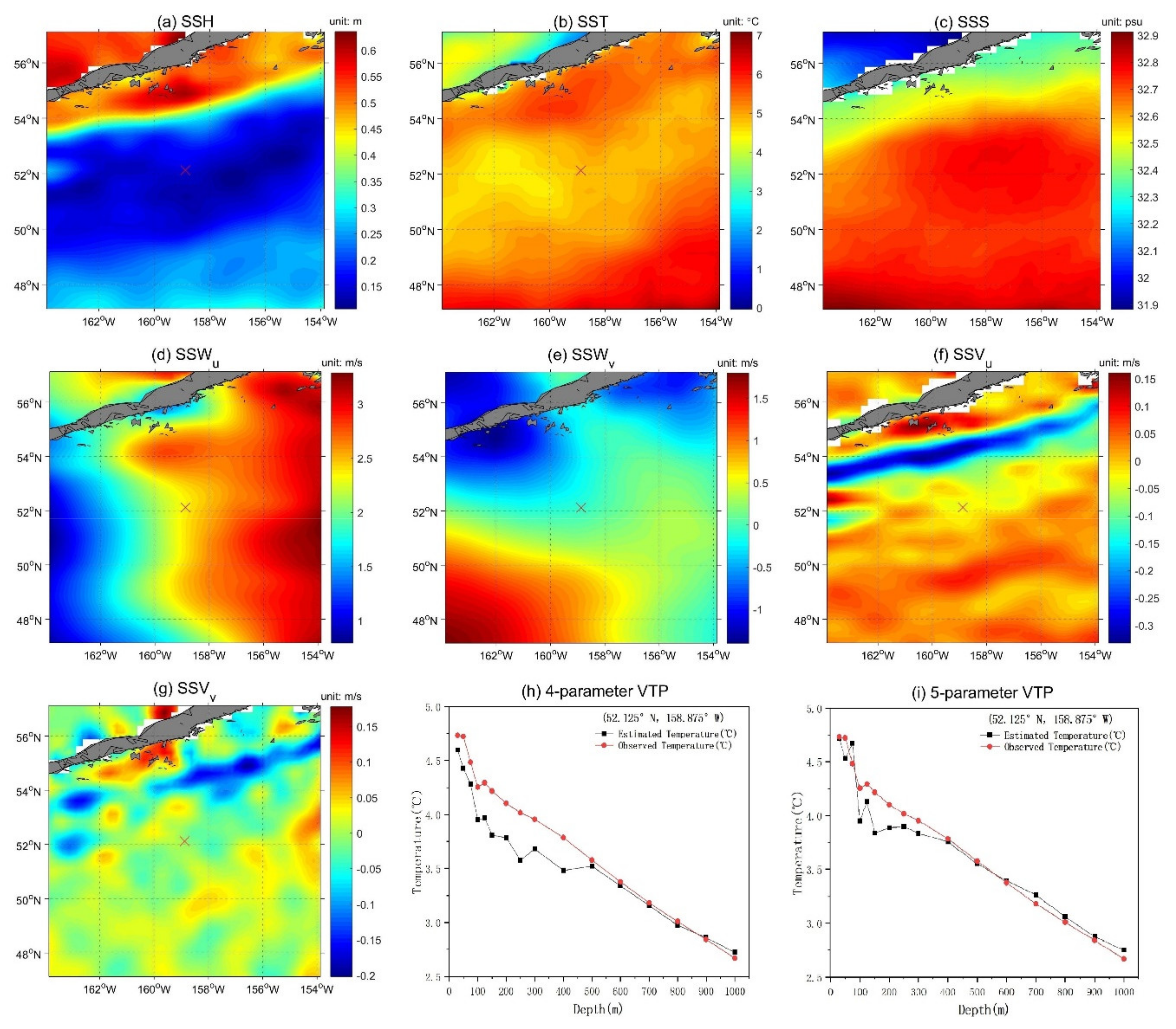
To further validate the reliability of the BPNN model at different depths, we randomly picked four pixels from the study area to compare the predicted vertical temperature profiles (VTP) with the observed temperature profiles (Figure 7). The four random pixels (case (a), (b), (c) and (d)) were located at 31.375° N, 132.625° E, 52.125° N, 158.875° W, 21.875° N, 174.125° E and 11.625° N, 128.125° W, respectively. The MSE and R² values of the four profiles were: MSE = 0.273, R² = 0.996 at (a); MSE = 0.079, R² = 0.882 at (b); MSE = 0.541, R² = 0.994 at (c); and MSE = 0.541, R² = 0.992 at (d). This indicates that there is a strong correlation between the temperature profiles predicted by the BPNN model and the observed temperature profiles. Figure 7 also shows that the four vertical profiles of the temperature estimated by the BPNN are generally consistent with the observations, which reflects the good performance of the BPNN model in the NPO. It should be noted that the estimated temperatures are significantly lower than observed temperatures between 100 and 300 m in Figure 7b. This may be related to the warming effect of the Alaska Current at that location.
To further explore the influence of the SSV on the results of the model estimation, we carried out comparative studies on cases (a) and (b). Figure 8 shows the sea surface parameters around case (a) and the VTP estimated by the four- and five-parameter models. Without a sea surface current, the MSE and R² values for case (a) calculated with the four-parameter model were 0.349 and 0.988, respectively. However, there is a strong Kuroshio Current in this region, which transports warmer and saltier water from low latitudes along the western boundary. The surface current velocity (Figure 8f,g) can be used to help calculate this transport. With this additional non-linear term, the estimated temperature is notably warmer (Figure 8i) than the previous result (Figure 8h), giving MSE and R² values of 0.273 and 0.996, respectively, with the five-parameters model.
Figure 9 shows the sea surface parameters around case (b) and the VTP estimated by the four- and five-parameters models. The MSE and R² values of case (b) calculated with the four-parameter model were 0.112 and 0.861, respectively (Figure 9h). Similar to case (a), there is a boundary current, but the current is much weaker than the Kuroshio Current. After taking the sea surface current into account, the estimated temperature is closer to the observed temperature, giving MSE and R² values of 0.079 and 0.882, respectively, using the five-parameter model (Figure 9i). Although the surface current velocity has a notable role, it is smaller than in case (a) because many mesoscale eddies propagate in a westerly direction along the Aleutian Islands [88]. The mesoscale eddies make the current much less stable, which leads to larger fluctuations in the estimated temperature (Figure 9i).
4. Discussion
Previous studies [1,65,66,67,68] have confirmed that the sea surface parameters SSH, SST, SSS and SSW can help in retrieving the thermal structure of the subsurface. We show here that the accuracy of the temperature estimation can be improved by adding the SSV as a variable on the basis of the existing SSH, SST, SST and SSW fields. Including more independent variables as input parameters of the model might therefore be a reasonable approach to improving the accuracy of the estimation. Variables such as the solar radiation and net heat flux [1] and the mixed-layer depth [89] might help to improve the accuracy of the estimation [90]. However, the computation requirements increase as the number of input variables increases and we therefore need to evaluate which variables are more effective in the estimation of temperature.
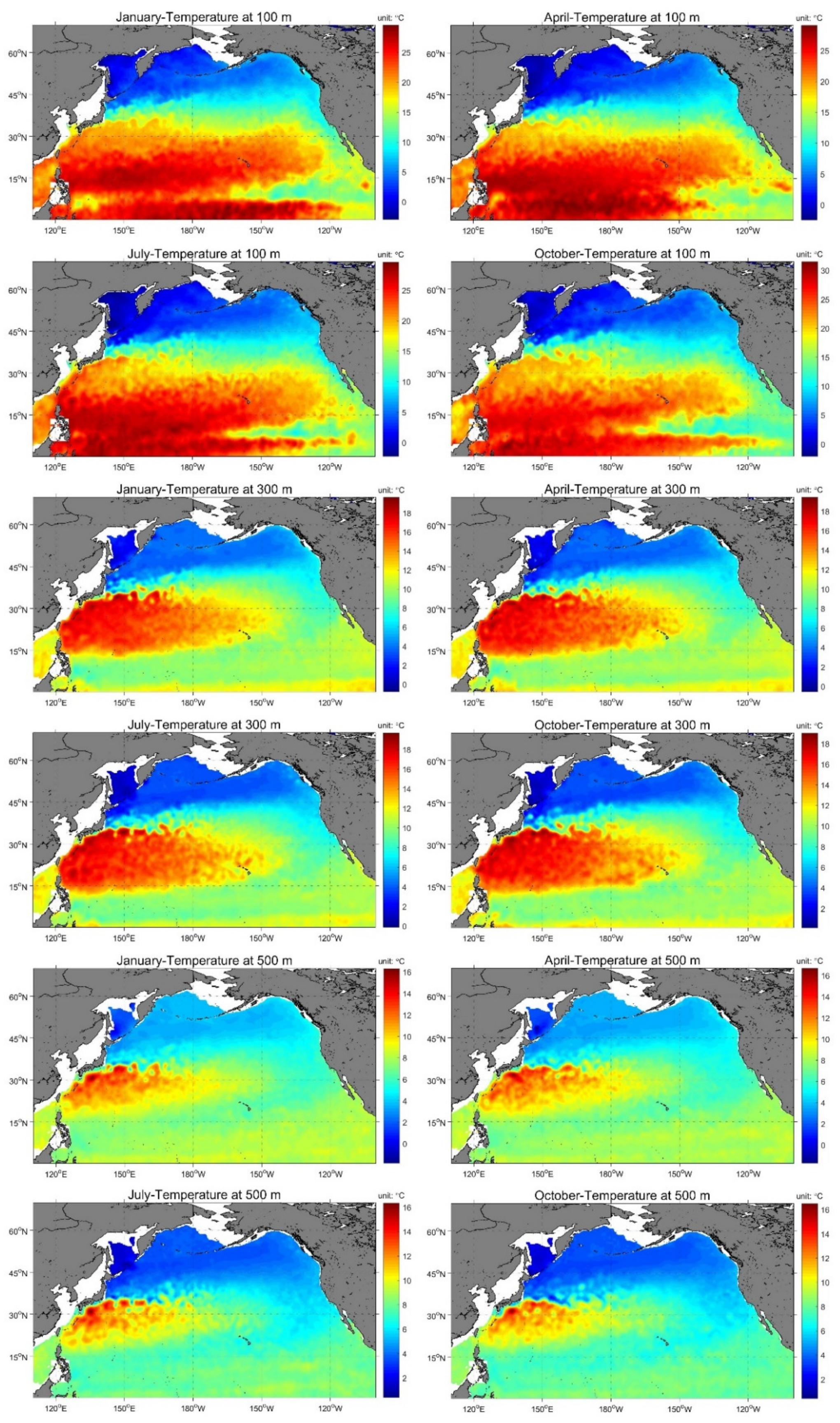
These results show a weaker seasonal variability of the deeper temperature fields than the natural variability (Figure 3 and Figure 4). Possible reasons for these weak seasonal signals are: (1) the original CMEMS training data lack seasonal variation signals; and (2) the BPNN model cannot correctly extract the seasonal signals that exist in the original training data. By analyzing the original target temperature field, we showed that the weak seasonal signal in these results is because the original target data lack seasonal variation signals (Figure 10). The state of the original target temperature field used for training therefore has an important impact on the results. We used model assimilation datasets for training. In future work, we will also consider using datasets combined with observational data from diverse sources, such as the training data, because the observed datasets can enhance the seasonal variation signal and might further improve the accuracy of the estimation.
The datasets also play an important role in model training and determine the range of application of the trained model. All the datasets used in this study are monthly mean values with the same spatial resolution of (0.25° × 0.25°) and therefore the model can reasonably estimate the subsurface temperature field with the same or lower resolution, but might not accurately capture signals with a higher temporal or spatial resolution. The temperatures estimated by the model are mostly confined to the temperature range used as the target, which means that if there is an abnormally high or low temperature in the study area, then this may be underestimated by the BPNN model. This might be solved by increasing the grid density and improving the computing power. Our trained model may have fitted well to the data source because the optimum weights of the model were trained by these datasets. However, datasets of the same variable obtained in different institutions may vary as a result of the different sources of the original data and different processing techniques. Therefore, the accuracy of the estimation may not be satisfactory when applying the trained BPNN model to other datasets and it would be better to use a combination of datasets from the same source as the application to train the model. In summary, the systematic errors of our model mainly came from the datasets we used and partly came from the network training parameters setting.
The Kling–Gupta efficiency (KGE) and Nash–Sutcliffe efficiency (NSE) are also commonly used statistical indexes in the evaluation of hydrological models [91,92,93,94]. Therefore, we firstly applied Equation (1) [91] to the four cases shown in Figure 7:
where r is the linear correlation between the observed and simulated temperatures, is the standard deviation of the estimated temperatures, is the standard deviation of the observed temperatures, is the estimated mean temperature and is the observed mean temperature. The KGE of cases (a), (b), (c), and (d) in Figure 7 are 0.969, 0.789, 0.933 and 0.986, respectively. Then, we use another four cases located at e (18.125° N, 141.125° E), f (28.375° N, 161.625° E), g (45.125° N, 166.375° W) and h (33.875° N, 129.875° W) to test the accuracy expressed by NSE. We use Equation (2) to calculate NSE since NSE and MSE are closely related [93]:
where is the standard deviation of the observed temperatures. The NSE values of the cases (e), (f), (g) and (h) are 0.9958, 0.9962, 0.8920 and 0.9737, respectively. The closer the KGE and NSE are to 1, the better the agreement between the estimations and observations. The model can therefore perform well under the metric of the KGE and NSE, which further verifies the stability of the model.
There is some concern about the performance of other machine learning methods when they are applied to relative studies. The advantage of unsupervised learning methods over supervised learning methods is the completion of training and adaptive clustering without labels. The SOM, a popular unsupervised learning algorithm in the field of computer vision, was applied to estimate the subsurface temperature in the North Atlantic and showed good performance in the depth range 30–700 m with a correlation coefficient of about 0.8 [63]. The results were not as good as those presented in this paper. This may be because, in addition to a lack of input parameters (SSW and SSV), the SOM algorithm itself is limited in estimating the subsurface temperature. SOM users must select the parameters, neighborhood function, grid type and centroid number before training, which introduces more artificial errors. Unlike a supervised learning method, the SOM method lacks a specific objective function. The BPNN method is therefore more suitable for regression analyses, such as subsurface temperature estimation, despite the advantages of the SOM in clustering analysis. The BPNN model is trained by machine learning algorithms and is essentially a fitting function. It is not restricted by physical mechanisms and may therefore cause unknown problems and instabilities. This might be a common failing of artificial intelligence methods in relative studies [63,65,66,67,90]. Future research should therefore consider coupling physical models with the data-driven machine learning model.
5. Conclusions
We introduced a BPNN method to estimate the internal temperature structure of the NPO based on sea surface parameters (SSH, SST, SSS, SSW and SSV). The BPNN method is one of the most popular machine learning methods and showed good performance in retrieving the thermal structure of the ocean subsurface. The estimated temperature field at each depth was verified by the observed temperature field and the accuracy of the estimation by the model was determined using the MSE and R² values. Our results show that the temperature estimation based on the BPNN model is both reliable and accurate. The correlation between the predicted and measured results was improved over those in previous models.
We analyzed the influence of different sea surface parameter combinations on the estimation of temperature through comparative experiments. In addition to the previously used variables (the SSH, SST, SSS and SSW) [1,63,64,65,66,67], we added the SSV as a new component and therefore the non-linear subsurface dynamics due to the advection associated with the SSV were taken into account. This improved the estimated temperature, especially in regions with a strong current. As a consequence, the accuracy of the BPNN model with five input parameters was higher than that of the BPNN model with four input parameters. This suggests that models with more sea surface parameters (e.g., the net heat flux) should be investigated to determine whether they can improve the accuracy of the model.
It should be noted that our results were sensitive to the original training data, which has a weaker seasonal variability than the in-situ data. This should be the general disadvantage of AI methods, that is, the accuracy of training data will affect the final output result. It is valuable to estimate how the error of original training data transmits along with the BPNN model to the final result, which could provide with us the uncertainty of the result in future. In addition, the temporal or spatial resolutions in this study may have missed some of the mesoscale dynamics, which can lead to extreme temperatures. These problems will be investigated in future work.
We developed a method to determine the thermal structure of the ocean interior based on the sea surface parameters measured by satellites. This study will help the development of deep-sea remote sensing technology based on machine learning and provide technical support for the construction of ocean observation datasets. This model provides a comprehensive understanding of the internal dynamics of the marine environment, which is crucial in studies of the global climate. However, the sea surface parameters used in the machine learning model are still limited and the dynamic mechanisms of the estimated results have not yet been explained. There is therefore still room to improve the accuracy of the estimation of the internal thermal structure of the ocean. Future work will consider the global-scale ocean with more surface datasets to retrieve internal parameters such as the 3D salinity and velocity fields. We will compare the results of our study with other approaches such as statistical methods and other machine learning methods to further verify the reliability and applicability of the proposed method. Advanced deep learning methods will be combined with dynamic methods to give more explanatory results.
Author Contributions
Conceptualization, H.C.; data curation, H.C.; formal analysis, H.C. and L.S.; funding acquisition, L.S.; investigation, H.C.; methodology, H.C.; project administration, L.S.; resources, L.S.; validation, J.L.; visualization, H.C.; writing—original draft, H.C.; writing—review and editing, L.S. and J.L. All authors have read and agreed to the published version of the manuscript.
Funding
This work was supported by the National Foundation of Natural Science of China (No. 41876013) and the National Program on Global Change and Air–Sea Interaction (GASI-IPOVAI-04).
Institutional Review Board Statement
Not applicable.
Informed Consent Statement
Not applicable.
Data Availability Statement
The SSH, SST, SSS, SSV data are openly available in Copernicus Marine and Environmental Monitoring Service (https://marine.copernicus.eu/). The CCMP SSW data are openly available in the Research Data Archive at the NCAR (https://rda.ucar.edu/datasets/ds745.1/).
Acknowledgments
We thank Copernicus Marine and Environmental Monitoring Service (CMEMS) for providing SSH, SST, SSS, SSV data (https://marine.copernicus.eu/), the Research Data Archive at the NCAR for the CCMP SSW data (https://rda.ucar.edu/datasets/ds745.1/), which are freely accessible for public. We are grateful to the anonymous reviewers whose comments and suggestions have helped improve the manuscript.
Conflicts of Interest
The authors declare no conflict of interest.
References
- Ali, M.M.; Swain, D.; Weller, R.A. Estimation of ocean subsurface thermal structure from surface parameters: A neural network approach. Geophys. Res. Lett. 2004. [Google Scholar] [CrossRef] [Green Version]
- Chapman, C.; Charantonis, A.A. Reconstruction of subsurface velocities from satellite observations using iterative self-organizing maps. IEEE Geosci. Remote Sens. 2017, 1, 617–620. [Google Scholar] [CrossRef]
- Guinehut, S.; Dhomps, A.L.; Larnicol, G.; Le Traon, P.Y. High resolution 3-D temperature and salinity fields derived from in situ and satellite observations. Ocean. Sci. 2012, 8, 845–857. [Google Scholar] [CrossRef] [Green Version]
- Wang, X.D.; Han, G.J.; Li, W.; Qi, Y.Q. Reconstruction of ocean temperature profile using satellite observations. J. Trop. Oceanogr. 2011, 30, 10–17. [Google Scholar]
- Vinogradova, N.; Lee, T.; Boutin, J.; Drushka, K.; Fournier, S.; Sabia, R.; Stammer, D.; Bayler, E.; Reul, N.; Gordon, A.; et al. Satellite salinity observing system: Recent discoveries and the way forward. Front. Mar. Sci. 2019, 6, 243. [Google Scholar] [CrossRef]
- Klemas, V.; Yan, X.H. Subsurface and deeper ocean remote sensing from satellites: An overview and new results. Prog. Oceanogr. 2014, 122, 1–9. [Google Scholar] [CrossRef]
- Meehl, G.A.; Arblaster, J.M.; Fasullo, J.T.; Hu, A.; Trenberth, K.E. Model-based evidence of deep-ocean heat uptake during surface-temperature hiatus periods. Nat. Clim. Chang. 2011, 1, 360–364. [Google Scholar] [CrossRef]
- Yan, X.H.; Boyer, T.; Trenberth, K.; Karl, T.R.; Xie, S.P.; Nieves, V.; Tung, K.K.; Roemmich, D. The global warming hiatus: Slowdown or redistribution? Earth’s Future 2016, 4, 472–482. [Google Scholar] [CrossRef]
- Bindoff, N.L.; Willebrand, J.; Artale, V.; Cazenave, A.; Gregory, J.M.; Gulev, S.; Hanawa, K.; Le Quere, C.; Levitus, S.; Nojiri, Y.; et al. Observations: Oceanic Climate Change and Sea Level. Climate Change 2007: The Physical Science Basis. Contribution of Working Group I; Cambridge University Press: Cambridge, UK, 2007; pp. 385–428. [Google Scholar]
- Balmaseda, M.A.; Trenberth, K.E.; Källén, E. Distinctive climate signals in reanalysis of global ocean heat content. Geophys. Res. Lett. 2013, 40, 1754–1759. [Google Scholar] [CrossRef]
- Song, Y.T.; Colberg, F. Deep ocean warming assessed fromaltimeters, gravity recovery and climate experiment, in situ measurements, and a non-Boussinesq ocean general circulation model. J. Geophys. Res. 2011, 116. [Google Scholar] [CrossRef] [Green Version]
- Chen, X.; Tung, K.K. Varying planetary heat sink led to global-warming slowdown and acceleration. Science 2014, 345, 897–903. [Google Scholar] [CrossRef] [PubMed]
- Drijfhout, S.S.; Blaker, A.T.; Josey, S.A.; Nurser, A.J.G.; Sinha, B.; Balmaseda, M.A. Surface warming hiatus caused by increased heat uptake across multiple ocean basins. Geophys. Res. Lett. 2014, 41, 7868–7874. [Google Scholar] [CrossRef] [Green Version]
- Levitus, S.; Antonov, J.I.; Boyer, T.P.; Locarnini, R.A.; Garcia, H.E.; Mishonov, A.V. Global ocean heat content 1955–2008 in light of recently revealed instrumentation problems. Geophys. Res. Lett. 2009, 36, 1–5. [Google Scholar] [CrossRef]
- Levitus, S.; Antonov, J.I.; Boyer, T.P.; Baranova, O.K.; Garcia, H.E.; Locarnini, R.A.; Zweng, M.M. World ocean heat content and thermosteric sea level change (0–2000 m), 1955–2010. Geophys. Res. Lett. 2012, 39, 1–5. [Google Scholar] [CrossRef] [Green Version]
- Lyman, J.M.; Good, S.A.; Gouretski, V.V.; Ishii, M.; Johnson, G.C.; Palmer, M.D.; Willis, J.K. Robust warming of the global upper ocean. Nature 2010, 465, 334–337. [Google Scholar] [CrossRef]
- Levin, L.A.; Le, B.N. The deep ocean under climate change. Science 2015, 350, 766–768. [Google Scholar] [CrossRef] [Green Version]
- Lowe, J.A.; Gregory, J.M.; Flather, R.A. Changes in the occurrence of storm surges around the United Kingdom under a future climate scenario using a dynamic storm surge model driven by the Hadley Centre climate models. Clim. Dynam. 2001, 18, 179–188. [Google Scholar] [CrossRef]
- Mel, R.; Sterl, A.; Lionello, P. High resolution climate projection of storm surge at the Venetian coast. Nat. Hazard. Earth Sys. 2013, 13, 1135–1142. [Google Scholar] [CrossRef] [Green Version]
- Woth, K.; Weisse, R.; Von, S.H. Climate change and North Sea storm surge extremes: An ensemble study of storm surge extremes expected in a changed climate projected by four different regional climate models. Ocean. Dynam. 2006, 56, 3–15. [Google Scholar] [CrossRef]
- Mel, R.; Lionello, P. Storm surge ensemble prediction for the city of Venice. Weather. Forecast. 2014, 29, 1044–1057. [Google Scholar] [CrossRef]
- Li, J.; Sun, L.; Yang, Y.; Yan, H.; Liu, S. Upper Ocean Responses to Binary Typhoons in the Nearshore and Offshore Areas of Northern South China Sea: A Comparison Study. J. Coast. Res. 2020, 99, 115–125. [Google Scholar] [CrossRef]
- Li, J.; Sun, L.; Yang, Y.; Cheng, H. Accurate Evaluation of Sea Surface Temperature Cooling Induced by Typhoons Based on Satellite Remote Sensing Observations. Water 2020, 12, 1413. [Google Scholar] [CrossRef]
- Liu, S.; Li, J.; Sun, L.; Wang, G.; Tan, D.; Huang, P.; Yan, H.; Gao, S.; Liu, C.; Gao, Z.; et al. Basin-wide responses of the South China Sea environment to Super Typhoon Mangkhut (2018). Sci. Total Environ. 2020, 731. [Google Scholar] [CrossRef] [PubMed]
- Wang, B.; Wu, R.; Li, T. Atmosphere–warm ocean interaction and its impacts on Asian–Australian monsoon variation. J. Clim. 2003, 16, 1195–1211. [Google Scholar] [CrossRef]
- Clemens, S.; Prell, W.; Murray, D.; Shimmield, G.; Weedon, G. Forcing mechanisms of the Indian Ocean monsoon. Nature 1991, 353, 720–725. [Google Scholar] [CrossRef]
- Turner, A.G.; Annamalai, H. Climate change and the South Asian summer monsoon. Nat. Clim. Change. 2012, 2, 587–595. [Google Scholar] [CrossRef]
- Zhisheng, A.; Guoxiong, W.; Jianping, L.; Youbin, S.; Yimin, L.; Weijian, Z.; Hai, C. Global monsoon dynamics and climate change. Annu. Rev. Earth Planet. Sci. 2015, 43, 29–77. [Google Scholar] [CrossRef] [Green Version]
- Loeb, N.G.; Lyman, J.M.; Johnson, G.C.; Allan, R.P.; Doelling, D.R.; Wong, T.; Stephens, G.L. Observed changes in top-of-the-atmosphere radiation and upper-ocean heating consistent within uncertainty. Nat. Geosci. 2012, 5, 110–113. [Google Scholar] [CrossRef]
- Fischer, M. Multivariate projection of ocean surface data onto subsurface sections. Geophys. Res. Lett. 2000, 27, 755–757. [Google Scholar] [CrossRef]
- Khedouri, E.; Szczechowski, C.; Cheney, R. Potential Oceanographic Applications of Satellite Altimetry for Inferring Subsurface Thermal Structure. In Proceedings, Oceans ’83: Technical Papers; IEEE: Piscataway, NJ, USA, 1983; pp. 274–280. [Google Scholar]
- Chu, P.C.; Fan, C.; Liu, W.T. Determination of Vertical Thermal Structure from Sea Surface Temperature. J. Atmos. Ocean. Tech. 2000, 17, 971–979. [Google Scholar] [CrossRef] [Green Version]
- Fox, D.N. The modular ocean data assimilation system. Oceanography 2002, 15, 22–28. [Google Scholar] [CrossRef]
- Guinehut, S.; Le Traon, P.Y.; Larnicol, G.; Philipps, S. Combining Argo and remote-sensing data to estimate the ocean three-dimensional temperature fields—A first approach based on simulated observations. J. Marine Syst. 2004, 46, 85–98. [Google Scholar] [CrossRef]
- Nardelli, B.B.; Guinehut, S.; Pascual, A.; Drillet, Y.; Ruiz, S.; Mulet, S. Towards high resolution mapping of 3-D mesoscale dynamics from observations: Preliminary comparison of retrieval techniques and models within MESCLA project. Ocean. Sci. 2012, 8, 885–901. [Google Scholar] [CrossRef] [Green Version]
- Carnes, M.R.; Mitchell, J.L.; Witt, P.W. Synthetic temperature profiles derived from Geosat altimetry: Comparison with air-dropped expendable bathythermograph profiles. J. Geophys. Res. Oceans 1990, 95, 17979–17992. [Google Scholar] [CrossRef]
- Carnes, M.R.; Teague, W.J.; Mitchell, J.L. Inference of subsurface thermohaline structure from fields measurable by satellite. J. Atmos. Ocean. Tech. 1994, 11, 551–566. [Google Scholar] [CrossRef] [Green Version]
- Nardelli, B.B.; Santoleri, R. Reconstructing synthetic profiles from surface data. J. Atmos. Ocean. Tech. 2004, 21, 693–703. [Google Scholar] [CrossRef]
- Nardelli, B.B.; Santoleri, R. Methods for the reconstruction of vertical profiles from surface data: Multivariate analyses, residual GEM, and variable temporal signals in the NPO. J. Atmos. Ocean. Tech. 2005, 22, 1762–1781. [Google Scholar] [CrossRef]
- Nardelli, B.B.; Cavalieri, O.; Rio, M.H.; Santoleri, R. Subsurface geostrophic velocities inference from altimeter data: Application to the Sicily Channel (Mediterranean Sea). J. Geophys. Res. Oceans 2006, 111. [Google Scholar] [CrossRef]
- Wang, H.; Wang, G.; Chen, D.; Zhang, R. Reconstruction of three-dimensional Pacific temperature with Argo and satellite observations. Atmos.-Ocean 2012, 50, 116–128. [Google Scholar] [CrossRef]
- Nardelli, B.B.; Guinehut, S.; Verbrugge, N.; Cotroneo, Y.; Zambianchi, E.; Iudicone, D. Southern Ocean mixed-layer seasonal and interannual variations from combined satellite and in situ data. J. Geophys. Res. Oceans 2017, 122, 10042–10060. [Google Scholar] [CrossRef] [Green Version]
- Nardelli, B.B.; Mulet, S.; Iudicone, D. Three-dimensional ageostrophic motion and water mass subduction in the Southern Ocean. J. Geophys. Res. Oceans 2018, 123, 1533–1562. [Google Scholar] [CrossRef]
- LaCasce, J.H.; Wang, J. Estimating subsurface velocities from surface fields with idealized stratification. J. Phys. Oceanogr. 2015, 45, 2424–2435. [Google Scholar] [CrossRef] [Green Version]
- Capet, X.; Roullet, G.; Klein, P.; Maze, G. Intensification of upper-ocean submesoscale turbulence through Charney baroclinic instability. J. Phys. Oceanogr. 2016, 46, 3365–3384. [Google Scholar] [CrossRef]
- Lapeyre, G. Surface quasi-geostrophy. Fluids 2017, 2, 7. [Google Scholar] [CrossRef]
- Klein, P.; Lapeyre, G.; Siegelman, L.; Qiu, B.; Fu, L.L.; Torres, H.; Su, Z.; Menemenlis, D.; Le Gentil, S. Ocean-scale interactions from space. Earth Space Sci. 2019, 6, 795–817. [Google Scholar] [CrossRef] [Green Version]
- Lapeyre, G.; Klein, P. Dynamics of the Upper Oceanic Layers in Terms of Surface Quasigeostrophy Theory. J. Phys. Oceanogr. 2006, 36, 165–176. [Google Scholar] [CrossRef]
- González, H.C.; Isern, F.J. Global Ocean current reconstruction from altimetric and microwave SST measurements. J. Geophys. Res. Oceans 2014, 119, 3378–3391. [Google Scholar] [CrossRef]
- Isern, F.J.; Chapron, B.; Lapeyre, G.; Klein, P. Potential use of microwave sea surface temperatures for the estimation of ocean currents. Geophys. Res. Lett. 2006, 33. [Google Scholar] [CrossRef] [Green Version]
- Isern, F.J.; Guillaume, L.; Klein, P.; Chapron, B.; Hecht, M.W. Three-dimensional reconstruction of oceanic mesoscale currents from surface information. J. Geophys. Res. 2008, 113. [Google Scholar] [CrossRef] [Green Version]
- Klein, P.; Lapeyre, G. The oceanic vertical pump induced by mesoscale and submesoscale turbulence. Annu. Rev. Mar. Sci. 2009, 1, 351–375. [Google Scholar] [CrossRef] [PubMed] [Green Version]
- Klein, P.; Hua, B.L.; Lapeyre, G.; Capet, X.; Gentil, S.L.; Sasaki, H. Upper ocean turbulence from high-resolution 3D simulations. J. Phys. Oceanogr. 2008, 38, 1748–1763. [Google Scholar] [CrossRef] [Green Version]
- Klein, P.; Isern-Fontanet, J.; Lapeyre, G.; Roullet, G.; Danioux, E.; Chapron, B. Diagnosis of vertical velocities in the upper ocean from high resolution sea surface height. Geophys. Res. Lett. 2009, 36. [Google Scholar] [CrossRef] [Green Version]
- Lapeyre, G. What vertical mode does the altimeter reflect? On the decomposition in baroclinic modes and on a surfacetrapped mode. J. Phys. Oceanogr. 2009, 39, 2857–2874. [Google Scholar] [CrossRef]
- Ponte, A.L.; Klein, P.; Capet, X.; Le Traon, P.Y.; Chapron, B.; Lherminier, P. Diagnosing surface mixed layer dynamics from high-resolution satellite observations: Numerical insights. J. Phys. Oceanogr. 2013, 43, 1345–1355. [Google Scholar] [CrossRef]
- Qiu, B.; Chen, S.; Klein, P.; Ubelmann, C.; Fu, L.L.; Sasaki, H. Reconstructability of three-dimensional upper-ocean circulation from SWOT sea surface height measurements. J. Phys. Oceanogr. 2016, 46, 947–963. [Google Scholar] [CrossRef]
- Wang, J.; Flierl, G.R.; LaCasce, J.H.; McClean, J.L.; Mahadevan, A. Reconstructing the ocean’s interior from surface data. J. Phys. Oceanogr. 2013, 43, 1611–1626. [Google Scholar] [CrossRef]
- Chen, Z.; Wang, X.; Liu, L. Reconstruction of three-dimensional ocean structure from sea surface data: An application of isQG method in the Southwest Indian Ocean. J. Geophys. Res. Oceans 2020, 125, 1–18. [Google Scholar] [CrossRef]
- Liu, L.; Peng, S.; Wang, J.; Huang, R. Retrieving density and velocity fields of the ocean’s interior from surface data. J. Geophys. Res. Oceans 2014, 119, 8512–8529. [Google Scholar] [CrossRef] [Green Version]
- Liu, L.; Peng, S.; Huang, R. Reconstruction of ocean’s interior from observed sea surface information. J. Geophys. Res. Oceans 2017, 122, 1042–1056. [Google Scholar] [CrossRef]
- Yan, H.; Wang, H.; Zhang, R.; Chen, J.; Bao, S.; Wang, G. A dynamical-statistical approach to retrieve the ocean interior structure from surface data: SQG-mEOF-R. J. Geophys. Res. Oceans 2020, 125, 1–15. [Google Scholar] [CrossRef]
- Wu, X.; Yan, X.H.; Jo, Y.H.; Liu, W.T. Estimation of subsurface temperature anomaly in the North Atlantic using a self-organizing map neural network. J. Atmos. Ocean. Tech. 2012, 29, 1675–1688. [Google Scholar] [CrossRef]
- Bao, S.; Zhang, R.; Wang, H.; Yan, H.; Yu, Y.; Chen, J. Salinity profile estimation in the Pacific Ocean from satellite surface salinity observations. J. Atmos. Ocean. Tech. 2019, 36, 53–68. [Google Scholar] [CrossRef]
- Su, H.; Wu, X.; Yan, X.H.; Kidwell, A. Estimation of subsurface temperature anomaly in the Indian Ocean during recent global surface warming hiatus from satellite measurements: A support vector machine approach. Remote Sens. Environ. 2015, 160, 63–71. [Google Scholar] [CrossRef]
- Su, H.; Li, W.; Yan, X.H. Retrieving temperature anomaly in the global subsurface and deeper ocean from satellite observations. J. Geophys. Res. Oceans 2018, 123, 399–410. [Google Scholar] [CrossRef]
- Su, H.; Huang, L.; Li, W.; Yang, X.; Yan, X.H. Retrieving Ocean Subsurface Temperature Using a Satellite-Based Geographically Weighted Regression Model. J. Geophys. Res. Oceans 2018, 123, 5180–5193. [Google Scholar] [CrossRef]
- Lu, W.; Su, H.; Yang, X.; Yan, X.H. Subsurface temperature estimation from remote sensing data using a clustering-neural network method. Remote Sens. Environ. 2019, 229, 213–222. [Google Scholar] [CrossRef]
- Ballabrera-Poy, J.; Mourre, B.; Garcia-Ladona, E.; Turiel, A.; Font, J. Linear and non-linear T–S models for the eastern North Atlantic from Argo data: Role of surface salinity observations. Deep Sea Res. Part I 2009, 56, 1605–1614. [Google Scholar] [CrossRef]
- Meijers, A.J.S.; Bindoff, N.L.; Rintoul, S.R. Estimating the four-dimensional structure of the Southern Ocean using satellite altimetry. J. Atmos. Ocean. Tech. 2011, 28, 548–568. [Google Scholar] [CrossRef]
- Zhang, K.; Geng, X.; Yan, X.H. Prediction of 3-D ocean temperature by multilayer convolutional LSTM. IEEE Geosci. Remote S. 2020, 17, 1303–1307. [Google Scholar] [CrossRef]
- Goh, A.T. Back-propagation neural networks for modeling complex systems. Artif. Intel. Eng. 1995, 9, 143–151. [Google Scholar] [CrossRef]
- Paola, J.D.; Schowengerdt, R.A. A detailed comparison of backpropagation neural network and maximum-likelihood classifiers for urban land use classification. IEEE Trans. Geosci. Remote Sens. 1995, 33, 981–996. [Google Scholar] [CrossRef]
- Paola, J.D.; Schowengerdt, R.A. A review and analysis of backpropagation neural networks for classification of remotely-sensed multi-spectral imagery. Int. J. Remote Sens. 1995, 16, 3033–3058. [Google Scholar] [CrossRef]
- Barnett, T.P.; Pierce, D.W.; Saravanan, R.; Schneider, N.; Dommenget, D.; Latif, M. Origins of the midlatitude Pacific decadal variability. Geophys. Res. Lett. 1999, 26, 1453–1456. [Google Scholar] [CrossRef] [Green Version]
- Di Lorenzo, E.; Schneider, N.; Cobb, K.M.; Franks, P.J.S.; Chhak, K.; Miller, A.J.; McWilliams, J.C.; Bograd, S.J.; Arango, H.; Curchitser, E.; et al. North Pacific Gyre Oscillation links ocean climate and ecosystem change. Geophys. Res. Lett. 2008, 35. [Google Scholar] [CrossRef] [Green Version]
- Pierce, D.W.; Barnett, T.P.; Latif, M. Connections between the Pacific Ocean tropics and midlatitudes on decadal timescales. J. Clim. 2000, 13, 1173–1194. [Google Scholar] [CrossRef]
- Collins, M.; An, S.I.; Cai, W.; Ganachaud, A.; Guilyardi, E.; Jin, F.F.; Jochum, M.; Lengaigne, M.; Power, S.; Timmermann, A.; et al. The impact of global warming on the tropical Pacific Ocean and El Niño. Nat. Geosci. 2010, 3, 391–397. [Google Scholar] [CrossRef]
- Brierley, A.S.; Kingsford, M.J. Impacts of climate change on marine organisms and ecosystems. Curr. Biol. 2009, 19, R602–R614. [Google Scholar] [CrossRef] [Green Version]
- Shepherd, T.G. Atmospheric circulation as a source of uncertainty in climate change projections. Nat. Geosci. 2014, 7, 703–708. [Google Scholar] [CrossRef]
- Nardelli, B.B.; Droghei, R.; Santoleri, R. Multi-dimensional interpolation of SMOS sea surface salinity with surface temperature and in situ salinity data. Remote Sens. Environ. 2016, 180, 392–402. [Google Scholar] [CrossRef]
- Miller, S.W.; Emery, W.J. An automated neural network and cloud classifier for use over land and ocean surfaces. J. Appl. Meteorol. 1997, 36, 1346–1362. [Google Scholar] [CrossRef]
- Bishop, C.M. Neural Networks for Pattern Recognition; Oxford University Press: Cambridge, UK, 1995; pp. 77–112. [Google Scholar]
- Funahashi, K.I. On the approximate realization of continuous mappings by neural networks. Neural Netw. 1989, 2, 183–192. [Google Scholar] [CrossRef]
- Karsoliya, S. Approximating number of hidden layer neurons in multiple hidden layer BPNN architecture. Inter. J. Eng. Trends. Tech. 2012, 3, 714–717. [Google Scholar]
- Maier, H.R.; Dandy, G.C. Neural networks for the prediction and forecasting of water resources variables: A review of modelling issues and applications. Environ. Modell. Softw. 2000, 15, 101–124. [Google Scholar] [CrossRef]
- Bowden, G.J.; Maier, H.R.; Dandy, G.C. Optimal division of data for neural network models in water resources applications. Water. Resour. Res. 2002, 38, 1–11. [Google Scholar] [CrossRef] [Green Version]
- Li, Q.Y.; Sun, L.; Lin, S.F. GEM: A dynamic tracking model for mesoscale eddies in the ocean. Ocean Sci. 2016, 12, 1249–1267. [Google Scholar] [CrossRef] [Green Version]
- Willis, J.K.; Roemmich, D.; Cornuelle, B. Combining altimetric height with broadscale profile data to estimate steric height, heat storage, subsurface temperature, and sea-surface temperature variability. J. Geophys. Res. Oceans 2003, 108. [Google Scholar] [CrossRef] [Green Version]
- Akbari, E.; Alavipanah, S.K.; Jeihouni, M.; Hajeb, M.; Haase, D.; Alavipanah, S. A review of ocean/sea subsurface water temperature studies from remote sensing and non-remote sensing methods. Water 2017, 9, 936. [Google Scholar] [CrossRef] [Green Version]
- Knoben, W.J.; Freer, J.E.; Woods, R.A. Inherent benchmark or not? Comparing Nash–Sutcliffe and Kling–Gupta efficiency scores. Hydrol. Earth Sys. Sci. 2019, 23, 4323–4331. [Google Scholar] [CrossRef] [Green Version]
- Mizukami, N.; Rakovec, O.; Newman, A.J.; Clark, M.P.; Wood, A.W.; Gupta, H.V.; Kumar, R. On the choice of calibration metrics for “high-flow” estimation using hydrologic models. Hydrol. Earth Sys. Sci. 2019, 23, 2601–2614. [Google Scholar] [CrossRef] [Green Version]
- Gupta, H.V.; Kling, H.; Yilmaz, K.K.; Martinez, G.F. Decomposition of the mean squared error and NSE performance criteria: Implications for improving hydrological modelling. J. Hydrol. 2009, 377, 80–91. [Google Scholar] [CrossRef] [Green Version]
- Pool, S.; Vis, M.; Seibert, J. Evaluating model performance: Towards a non-parametric variant of the Kling-Gupta efficiency. Hydrol. Sci. J. 2018, 63, 1941–1953. [Google Scholar] [CrossRef]
Figure 1.
Surface parameters and temperature at 500 m depth in the study area with a spatial resolution of 0.25° × 0.25° in March 2015. The sea surface wind (SSW)u, SSWv, sea surface velocity (SSV)u and SSVv are the meridional and latitudinal components of the SSW and SSV, respectively.
Figure 1.
Surface parameters and temperature at 500 m depth in the study area with a spatial resolution of 0.25° × 0.25° in March 2015. The sea surface wind (SSW)u, SSWv, sea surface velocity (SSV)u and SSVv are the meridional and latitudinal components of the SSW and SSV, respectively.

Figure 2.
Flow chart of the back-propagation neural network (BPNN) approach for the estimation of subsurface temperatures at different depths (e.g., 500 m depth). The sea surface height (SSH), sea surface temperature (SST), sea surface salinity (SSS), SSW and SSV datasets were used for training and the SSHp, SSTp, SSSp, SSWp and SSVp datasets were used for estimation.

Figure 3.
Estimated temperature based on five sea surface parameters (SSH, SST, SSS, SSW and SSV) compared with the observed temperature at different depths (a1) and (a2) for 100 m; (b1) and (b2) for 300 m; (c1) and (c2) for 500 m; (d1) and (d2) for 700 m; (e1) and (e2) for 1000 m) in the North Pacific Ocean (NPO) during January 2015.

Figure 4.
Estimated temperature based on five sea surface parameters (SSH, SST, SSS, SSW, SSV) compared with the observed temperature at different depth levels (a1) and (a2) for 100 m; (b1) and (b2) for 300 m; (c1) and (c2) for 500 m; (d1) and (d2) for 700 m; (e1) and (e2) for 1000 m) in the NPO during July 2015.

Figure 5.
Evaluation of the accuracy of the temperature estimation results at 16 different depths in the NPO based on the BPNN model. MSE5 and MSE4 are the MSE for the five- and four-parameter BPNN model; R²5 and R²4 are R² for the five- and four-parameter BPNN model, respectively.
Figure 5.
Evaluation of the accuracy of the temperature estimation results at 16 different depths in the NPO based on the BPNN model. MSE5 and MSE4 are the MSE for the five- and four-parameter BPNN model; R²5 and R²4 are R² for the five- and four-parameter BPNN model, respectively.

Figure 6.
Density scatter plots of the correlation between the temperature estimated by the five-parameter BPNN model and the observed temperature at different depths (a) for 200 m; (b) for 400 m; (c) for 600 m; (d) for 800 m.
Figure 6.
Density scatter plots of the correlation between the temperature estimated by the five-parameter BPNN model and the observed temperature at different depths (a) for 200 m; (b) for 400 m; (c) for 600 m; (d) for 800 m.

Figure 7.
Vertical temperature profiles (VTP) ((a) for case (a); (b) for case (b); (c) for case (c); (d) for case (d)) of four randomly selected pixels at 16 different depths during March 2015.
Figure 7.
Vertical temperature profiles (VTP) ((a) for case (a); (b) for case (b); (c) for case (c); (d) for case (d)) of four randomly selected pixels at 16 different depths during March 2015.

Figure 8.
(a–g) are surface parameters around case (a) and (h–i) are VTP with the four- and five-parameter models during March 2015.
Figure 8.
(a–g) are surface parameters around case (a) and (h–i) are VTP with the four- and five-parameter models during March 2015.

Figure 9.
(a–g) are surface parameters around case (b) and (h–i) are VTP with the four- and five-parameter models during March 2015.
Figure 9.
(a–g) are surface parameters around case (b) and (h–i) are VTP with the four- and five-parameter models during March 2015.

Figure 10.
Temperature fields at 100, 300 and 500 m depth in four seasons (using January, April, July and October to represent winter, spring, summer and autumn).
Figure 10.
Temperature fields at 100, 300 and 500 m depth in four seasons (using January, April, July and October to represent winter, spring, summer and autumn).


Table 1.
Mean square error (MSE) and coefficient of determination (R²) of the BPNN model with five and four input parameters at 16 different depths.
Table 1.
Mean square error (MSE) and coefficient of determination (R²) of the BPNN model with five and four input parameters at 16 different depths.
| Depth (m) | MSE (SSH, SST, SSS, SSW, SSV)/(SSH, SST, SSS, SSW)/Difference | R² (SSH, SST, SSS, SSW, SSV)/(SSH, SST, SSS, SSW)/Difference |
|---|---|---|
| 30 | 0.895/0.908/−0.013 | 0.988/0.988/0 |
| 50 | 1.605/1.852/−0.247 | 0.980/0.974/0.006 |
| 75 | 1.931/1.996/−0.065 | 0.974/0.968/0.006 |
| 100 | 1.970/2.125/−0.155 | 0.970/0.962/0.008 |
| 125 | 1.911/2.014/−0.103 | 0.966/0.955/0.011 |
| 150 | 1.612/1.754/−0.142 | 0.962/0.943/0.019 |
| 200 | 0.895/0.967/−0.072 | 0.968/0.951/0.017 |
| 250 | 0.545/0.642/−0.097 | 0.970/0.955/0.015 |
| 300 | 0.462/0.504/−0.042 | 0.968/0.966/0.002 |
| 400 | 0.397/0.421/−0.024 | 0.958/0.953/0.005 |
| 500 | 0.284/0.296/−0.012 | 0.951/0.945/0.006 |
| 600 | 0.146/0.196/−0.050 | 0.949/0.939/0.010 |
| 700 | 0.079/0.082/−0.003 | 0.945/0.935/0.010 |
| 800 | 0.049/0.067/−0.018 | 0.943/0.933/0.010 |
| 900 | 0.037/0.041/−0.004 | 0.939/0.933/0.006 |
| 1000 | 0.028/0.029/−0.001 | 0.935/0.931/0.004 |
Publisher’s Note: MDPI stays neutral with regard to jurisdictional claims in published maps and institutional affiliations. |
© 2021 by the authors. Licensee MDPI, Basel, Switzerland. This article is an open access article distributed under the terms and conditions of the Creative Commons Attribution (CC BY) license (http://creativecommons.org/licenses/by/4.0/).
Share and Cite
MDPI and ACS Style
Cheng, H.; Sun, L.; Li, J. Neural Network Approach to Retrieving Ocean Subsurface Temperatures from Surface Parameters Observed by Satellites. Water 2021, 13, 388. https://doi.org/10.3390/w13030388
AMA Style
Cheng H, Sun L, Li J. Neural Network Approach to Retrieving Ocean Subsurface Temperatures from Surface Parameters Observed by Satellites. Water. 2021; 13(3):388. https://doi.org/10.3390/w13030388
Chicago/Turabian StyleCheng, Hao, Liang Sun, and Jiagen Li. 2021. "Neural Network Approach to Retrieving Ocean Subsurface Temperatures from Surface Parameters Observed by Satellites" Water 13, no. 3: 388. https://doi.org/10.3390/w13030388
Note that from the first issue of 2016, this journal uses article numbers instead of page numbers. See further details here.