Article

Structural Changes in French VF Treatment Wetland Porous Media during the Rest Period: An Ex Situ Study Using X-ray Tomography

by
German Dario Martinez-Carvajal
1,
Laurent Oxarango
2,
Jérôme Adrien
3,
Pascal Molle
4 and
Nicolas Forquet
4,*
1
Institut Blaise Pascal, 4 Avenue Blaise Pascal TSA 60026/CS 60026, CEDEX, 63178 Aubière, France
2
CNRS, IRD, Grenoble INP, IGE, Université Grenoble Alpes, 38000 Grenoble, France
3
INSA-Lyon, MATEIS Laboratory, University of Lyon, UMR CNRS 5510, 20 Avenue Albert Einstein, CEDEX, 69621 Villeurbanne, France
4
UR REVERSAAL, INRAE 5 rue de la Doua-CS70077, 69626 Villeurbanne, France
*
Author to whom correspondence should be addressed.
Water 2021, 13(3), 389; https://doi.org/10.3390/w13030389
Submission received: 4 December 2020 / Revised: 27 January 2021 / Accepted: 27 January 2021 / Published: 2 February 2021
(This article belongs to the Section Wastewater Treatment and Reuse)

Abstract

:
Clogging constitutes a major operational issue for treatment wetlands. The rest period is a key feature of French Vertical Flow (VF) treatment wetlands and serves to mitigate clogging. An ex-situ drying experiment was performed to mimic the rest period and record structural changes in the porous media using X-ray Computed Tomography (CT). Samples containing the deposit and gravel layers of a first stage French VF treatment wetland were extracted and left to dry in a control environment. Based on CT scans, three phases were identified (voids, biosolids, and gravels). The impact of the rest period was assessed by means of different pore-scale variables. Ultimately, the volume of biosolids had reduced to 58% of its initial value, the deposit layer thickness dropped to 68% of its initial value, and the void/biosolid specific surface area ratio increased from a minimum value of 1.1 to a maximum of 4.2. Cracks greater than 3 mm developed at the uppermost part of the deposit layer, while, in the gravel layer, the rise in void volume corresponds to pores smaller than 2 mm in diameter. Lastly, the air-filled microporosity is estimated to have increased by 0.11 v/v.

Graphical Abstract

1. Introduction

French Vertical Flow (VF) treatment wetlands have become a popular technology to treat domestic wastewater for communities under 5000 people equivalent (p.e.) in France [1]. French VF treatment wetlands consist of an arrangement of filters in two successive stages planted with Phragmites Australis. The first stage filters receive raw wastewater in intermittent batches over 3.5 days and then rest for 7 days; three filters are sequentially fed to ensure continuous wastewater treatment. These filters are filled with a coarse granular material (2–4 mm gravel) that allows retaining Suspended Solids (SS). In being fed by raw wastewater, they develop a surface deposit layer [2] after few years in operation. SS are mainly retained by deep bed filtration [3] in newly commissioned filters, as well as by cake filtration once the deposit layer has developed.
The deposit layer helps establish a homogeneous distribution of the influent over the treatment wetland surface during a given batch. Moreover, it is thought to be the seat of most biological processes that reduce the concentration of pollutants, including the degradation of Organic Matter (OM) and nitrification provided effective oxygenation can be ensured [2]. Once this layer reaches a thickness of 20 cm, its removal is recommended in order to renew the infiltration capacity of filters and prevent overflow. At the time of their removal, solids from the deposit layer show a high level of mineralization and stability, which makes the layer suitable for agricultural purposes [4].
Clogging and fouling, resulting from the accumulation of solids in the filters, are two major concerns in treatment wetland performance and operations. The literature however only contains a few works providing a practical definition of clogging, the degree of clogging [5], and its difference with fouling, especially in the context of French VF treatment wetlands. Pucher and Langergraber [5] suggest that a filter should be considered clogged if the volume of water received during a batch does not completely infiltrate before the subsequent batch, moreover, the degree of clogging can be defined as a function of the percentage of the filter surface permanently ponded during two consecutive batches. However, this definition only applies to filters permanently fed and proves to be ill-suited for French VF treatment wetlands, in which ponding duration varies during a feeding period with a strong seasonality effect. The following distinction is therefore preferred in the context of French VF treatment wetlands: a filter is considered clogged if the reduction in infiltration rate leads to overflows or degraded treatment. In contrast, a fouled French VF treatment wetland retains a certain amount of solids within both the filtering gravel layer and deposit layer yet without compromising treatment efficiency. This solid accumulation is herein referred to as biosolids. The biosolids contained in the gravel and deposit layers play an important role in wastewater treatment as a seat of the microorganisms and fauna responsible for organic matter degradation. Biosolids are characterized by their high organic matter content, which ranges from 50% to nearly 90% [6] and forms a porous medium in which its structure and consistency evolve over time due to water content changes, organic matter mineralization, erosion and bioturbation.
The rest period avoids over-accumulation of biosolids, which could transition the treatment wetland to a clogged state. During this period, the water content and volume of biosolids decrease through drainage, evapotranspiration and mineralization. Biosolids drying leads to shrinkage and cracking, which in turn facilitate oxygen diffusion into the filter and aerobic mineralization.
Understanding the underpinnings of solid transport and its biodegradation is necessary in order to optimize the design and operating rules of French VF treatment wetlands, especially in scenarios aimed at reducing the footprint of the technology or predicting its lifespan. Although the duration of the feeding and rest periods in Reference [4] has been statistically proven to ensure a good treatment performance in French VF treatment wetlands [1], these rules remain mainly empirical [7] and could be optimized. In addition, a mechanistic description of the physical and biological processes in French VF treatment wetlands is key to both understanding the dynamics of clogging, and finding solutions in cases where clogging has occurred prematurely. Taken as a whole, this description would improve the reliability and sustainability of the French VF treatment wetland technology.
Clogging is strongly correlated with the physical, chemical, biological and hydraulic processes in French VF treatment wetlands. Consequently, various methodologies to assess clogging in treatment wetlands are cited in the literature and based on the measurement and monitoring of several variables or properties related to these processes, including: (free)-porosity, solid densities, resistance to erosion, Specific Surface Areas (SSA), chemical composition of biosolids, water infiltration rate, in/ex-situ water permeability, water content, water residence time, oxygen consumption rate, enzymatic activity, oxydo-reduction potential, and even DNA sequencing [8]. However, fouling and clogging are phenomena that basically consist of filling a void volume by biosolids, where both their amount and geometric distribution are critical.
Only three methodologies that assess clogging/fouling in treatment wetlands and rely on a geometric description are reported in the literature, namely: geo-endoscopy [9], thin sections [10], and X-ray Tomography [11]. Geo-endoscopy yields (2D) images 6 mm high and 5 mm wide with a resolution of 10 μ m·pixel 1 and capable of capturing the vertical profile of solids along with the porosity filling level in a filter along a borehole. Thin sections are wider (5 cm × 7 cm); hence, their resolution can reach values of 1 μ m·pixel 1 , which makes it possible to observe the biosolid microporosity. However, their production requires the use of organic solvents to replace water in the samples, which in turn may alter the biosolid structure, especially in the deposit layer [12]. X-ray Computed Tomography (X-ray CT) can yield 3D-morphological descriptions of larger volumes of treatment wetland samples without any pretreatment. The resolution offers a compromise between sample size on the one hand and the size and number of active cells in the X-ray sensor on the other. High-level image processing algorithms are required to process the images generated by X-ray CT.
Recent works on the application of X-ray CT to study French VF treatment wetlands have demonstrated the feasibility and spatial representativy of this methodology [11,13], which sets a solid basis for use in studying dynamic phenomena, such as the drying that occurs during the rest period. X-ray CT seems to be a suitable methodology to evaluate the structural changes taking place in French VF treatment wetlands during the rest period for several reasons: (1) it is by far the most widespread methodology for deriving good morphological descriptions of porous media [14], (2) it produces a realistic (3D) morphological description, (3) it serves as a non destructive technique, necessitating no pretreatment procedure to obtain images of samples from French VF treatment wetlands, and (4) it has already been successfully used to study the dynamics of drying in other types of porous media [15,16,17,18].
Methodologies, like X-ray CT, are used to estimate properties of filtering media (e.g., porosity, effective transfer coefficients, and water permeability) based on a realistic description of its pore structure [19,20]. This upscaling approach differs from global approaches for which filtering media properties are often obtained by calibration. The major concern when studying the filtering media at the pore scale is the spatial representativity of the measurements and it remains an openly discussed topic in the scientific community. Different approaches and methodologies have been proposed to assess the Representative Elementary Volume (REV), which is the volume at which the averaged value of a property is no longer dependent on the size of the sample [21,22,
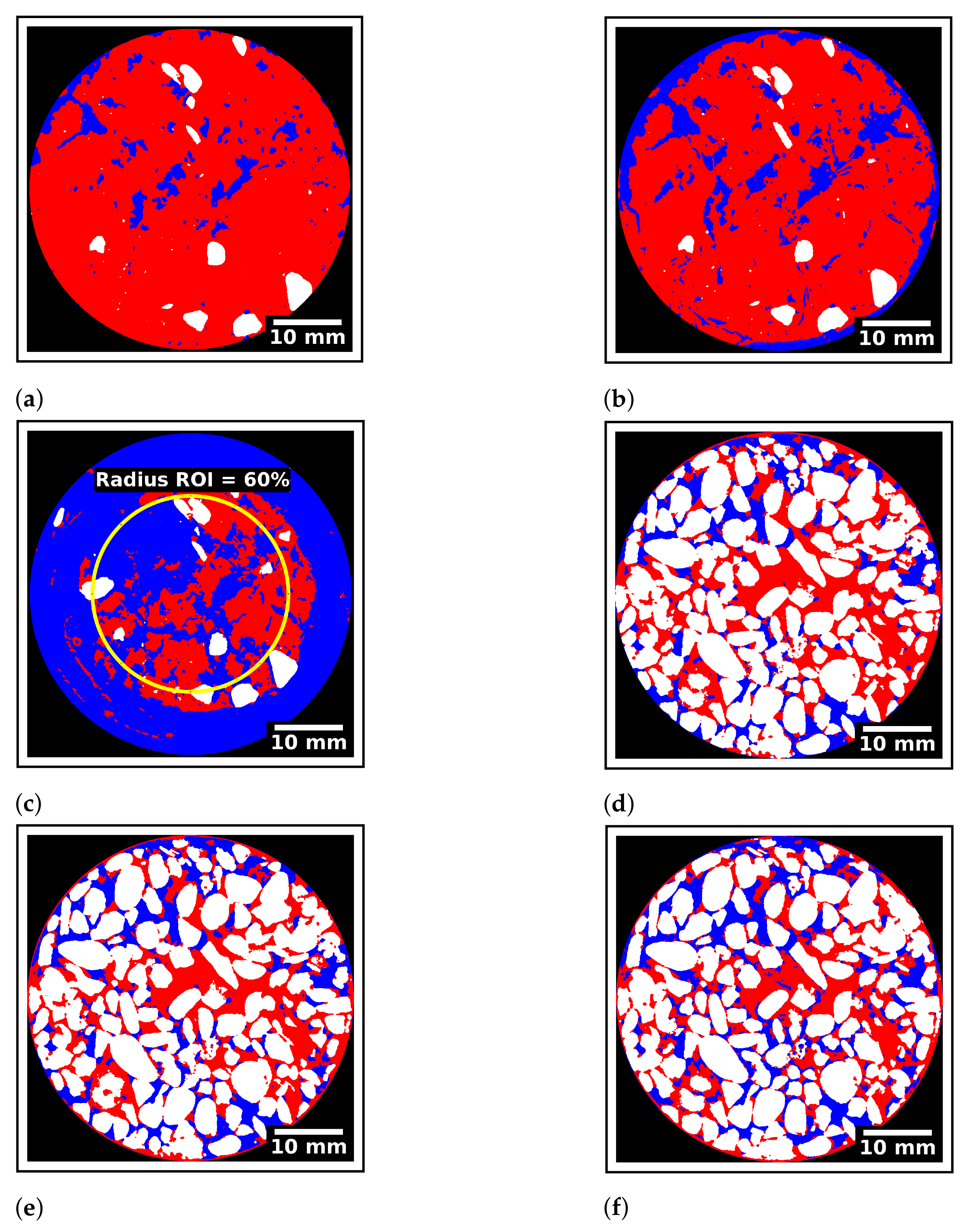
23]. A recent study on the assessment of spatial representativity of X-ray CT for the study of VFTW showed that samples 5 cm in diameter are large enough to be representative of the heterogeneous volumetric distribution of all the phases (voids, biosolids, and gravel) as long as no reed is present [13].
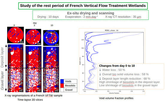
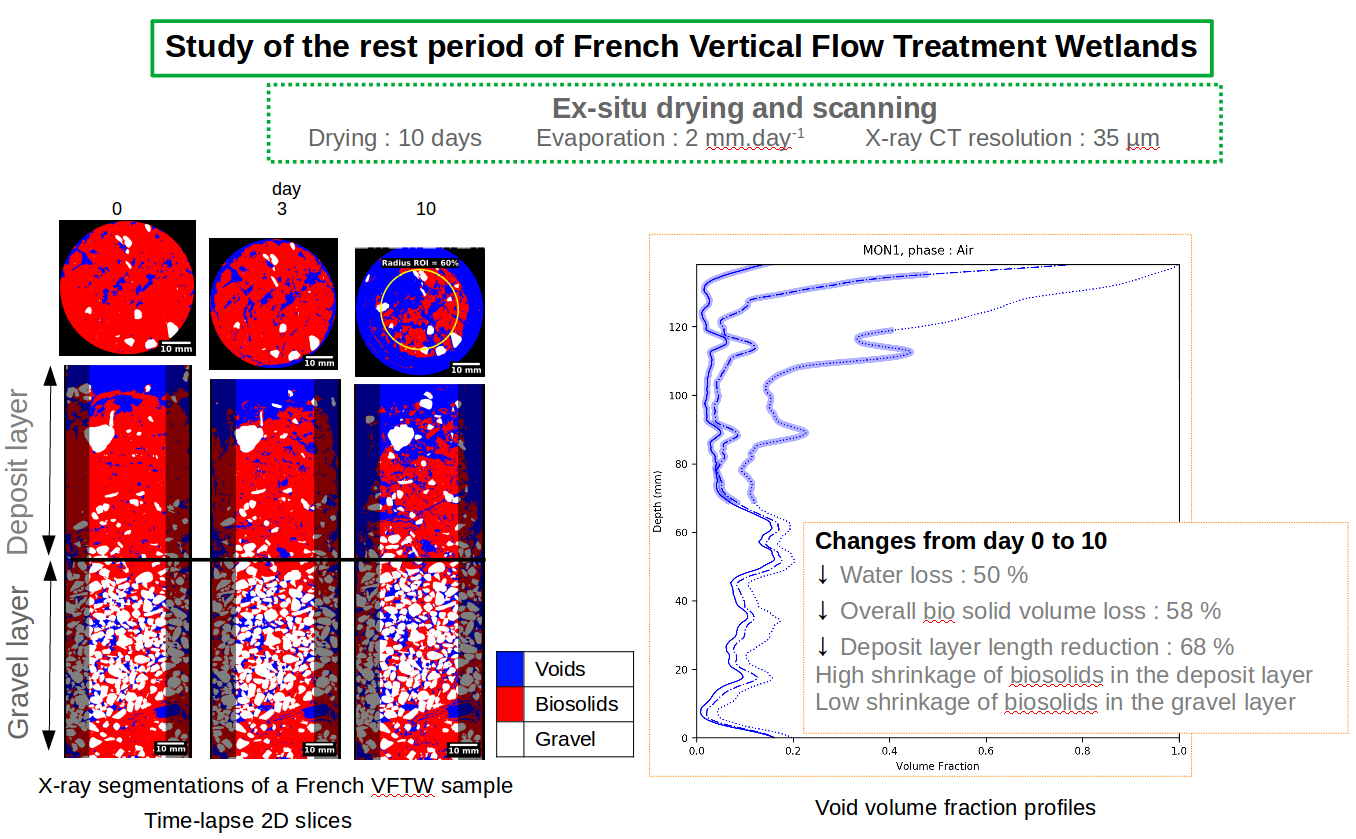
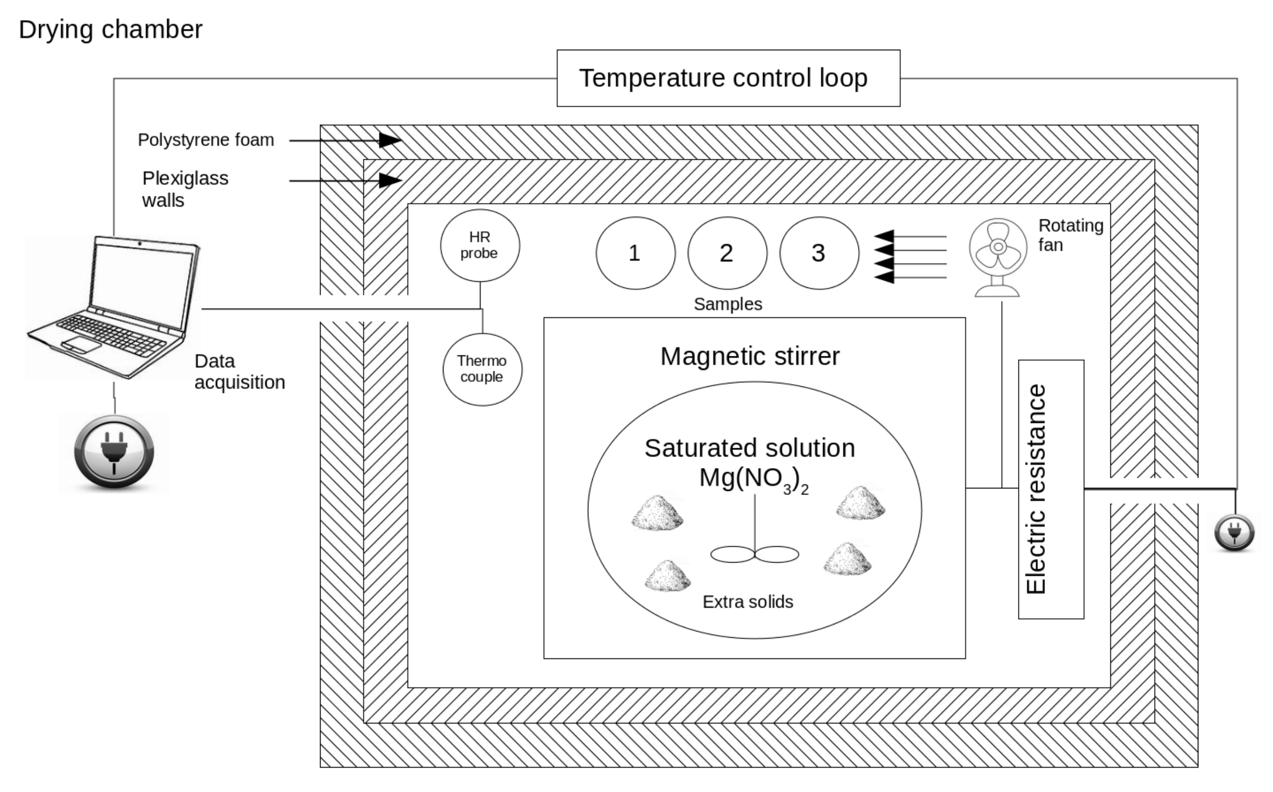
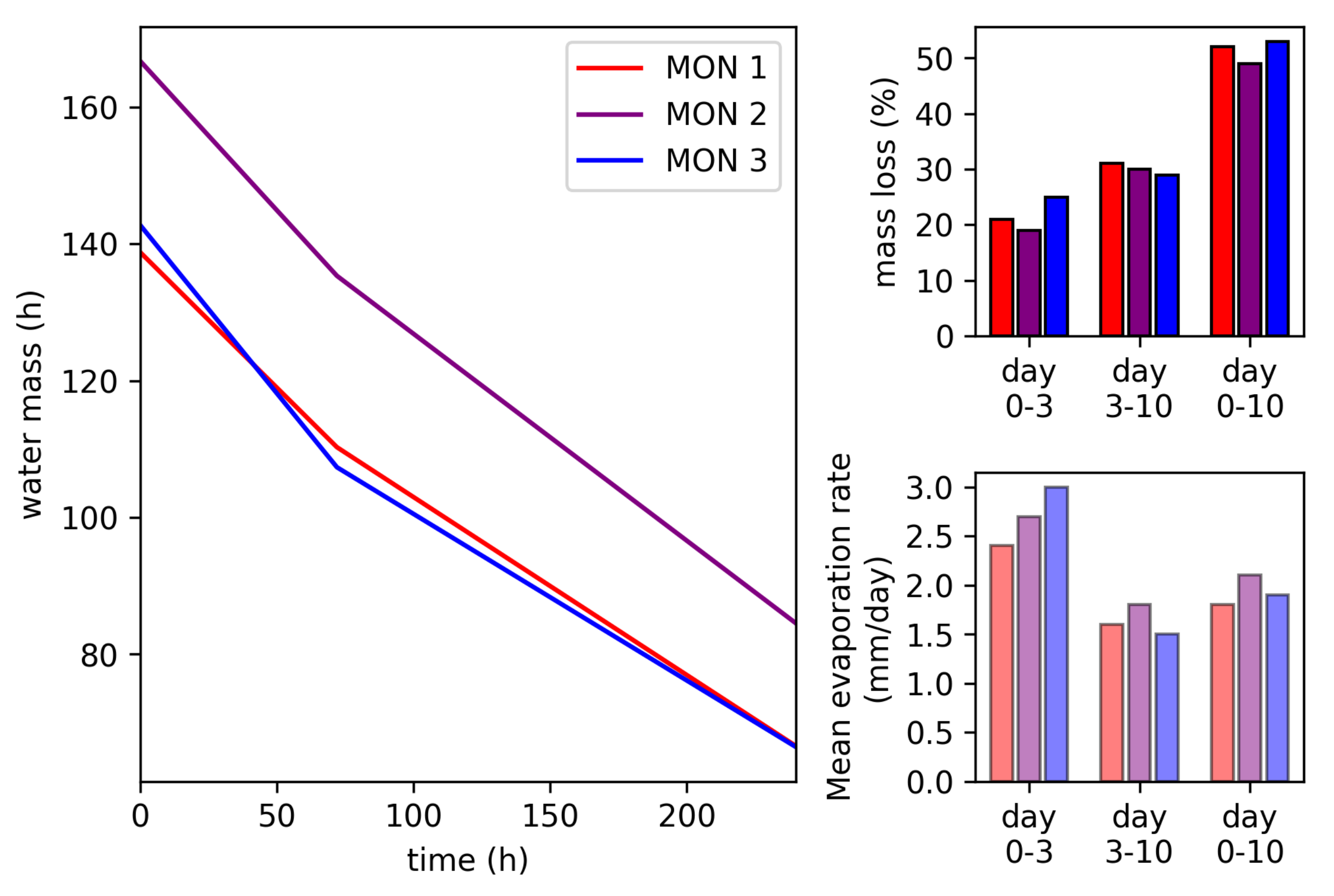
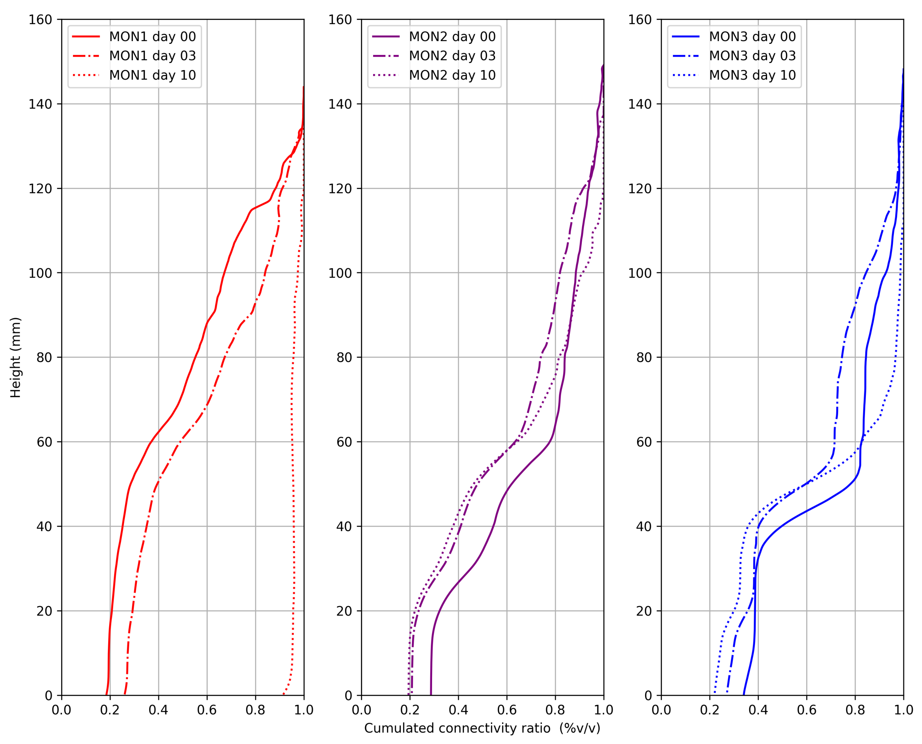
This work carries out an ex situ drying experiment simulating the rest period of a French VF treatment wetland. Three samples from a full scale treatment wetland were left to dry in a closed chamber under controlled conditions of temperature and relative humidity. X-ray CT scans were performed at three different times over a 10-day period. The aim of this experiment was to evaluate how drying affects macropores within the filtering material, as well as their size and connectivity, since this step is believed to be the primary means by which oxygen diffuses into the biosolids and their micropores. We consider here micropores to be voids smaller than 35 µm (scan resolution).

2. Materials and Methods

2.1. Study Site

The French VF treatment wetland in Montromant (Rhône, France) was chosen to carry out this study; the site was designed according to French standards presented in Reference [4] to treat effluent from 200 p.e.; it features two treatment stages, consisting of four filters in parallel for the first stage and two filters in parallel for the second. Since the facility was commissioned in 1994, three of the four filters in the first stage have been in operation. In 2009, the deposit layer of these filters was removed and the fourth filter of the first stage was put into operation. The duration of the feeding period remained 3.5 days, and the rest period was then extended to 10.5 days. A recent assessment of the distribution of biosolids at the wetland surface was performed in one of the oldest first-stage filters in operation using the Frequency Domain Electromagnetic Method (FDEM) [13]. The results of this study suggested that the biosolid distribution in this wetland is homogeneous over nearly 95% of the surface. No significant differences in the global content of biosolids are expected in the samples extracted from this area.

2.2. Sampling

Three samples were extracted from three distinct locations inside a homogeneous area delimited by FDEM [13] at the end of a feeding period in November 2018. They were labeled MON1, MON2, and MON3. Each sample consisted of a Poly(methyl methacrylate) (PMMA) cylinder 5 cm in diameter and 16 cm high. The samples were tall enough to contain the entire deposit layer and a portion of the dense gravel layer beneath. To extract the samples, an area was cleared of reed stems at the sampling points. The cylinder was then manually inserted. As the cylinder was being buried into the filter, the gravels surrounding it had to be progressively dug out at the same time, and any rhizome found was cut to avoid compaction and changes in sample structure [11]. After extraction, all samples were sealed with a plastic film and stored at 5 °C to prevent water evaporation before the beginning of the ex situ drying experiment.

2.3. Ex Situ Drying Experiment

The drying of biosolids during the rest period of a French VF treatment wetland is mainly driven by evapotranspiration. An ex situ (laboratory) study of the rest period using X-ray CT has the following practical advantages: (1) the variables influencing drying can be easily controlled; (2) the experiment is not adversely affected by stochastic events, like rain, which would alter results if several samples were to be extracted at different times during an in situ rest period; and (3) the comparison of structural changes is easier to perform if the same samples are scanned over the entire study. In such an experiment, the drying conditions, especially temperature and relative humidity of the atmosphere, must be carefully set to counterbalance the fact that mature reeds will not contribute to evapotranspiration.
An ad-hoc PMMA drying chamber was built to maintain the samples under constant temperature and relative humidity conditions (see Figure 1) during the experiment. This chamber measured 90 × 50 × 40 cm 3 (l × w × h) and was covered with a 3-cm thick layer of polystyrene foam to provide thermal insulation. The samples were placed inside and dried for 10 days, (i.e., the duration of the rest period at Montromant’s French VF treatment wetland). Only the upper part of the sample was in direct contact with the chamber atmosphere. An 80-W electrical resistance heater, regulated by a thermocouple, served to maintain the chamber temperature around the set value of 25 °C. The average temperature outside the chamber was 21 °C. Three liters of a saturated solution of Mg ( NO 3 ) 2 with an extra 200 g of salt was used to maintain relative humidity in the chamber at close to the equilibrium value of 50%. The solution was continuously stirred. A rotating fan with blades 85 mm in diameter and producing an air current of 3.33 m/s (measured by a portable anemometer-GEOS n°11, Skywatch) was operated to homogenize temperature, and relative humid by rapidly mixing the humid air at the top of the samples with the chamber atmosphere. The temperature and relative humidity were continuously monitored and the sample masses were measured once a day during the experiment. Evaporation rates were computed by dividing the daily mass losses by the sample surface area (19.63 cm 2 ).

2.4. Gravimetric Measurements

At the end of the drying period, the total water content, Volatile Suspended Solids (VSS), ashes, and gravel mass for each sample were estimated by means of a gravimetric analysis. The total water content was obtained by computing the difference between the initial sample mass and the mass after 24 h of drying at 105 °C. VSS were computed as the mass loss after calcination of the samples at 550 °C. The solids remaining after calcination, consisting of a mixture of gravel and ash aggregates from the biosolids, were then separated using a 0.63 mm sieve. To facilitate sieving, the ash aggregates were manually broken.

2.5. X-ray Tomography, Image Pretreatment and Segmentation

A tomography of each sample was performed at days 0, 3 and 10 of the ex situ drying experiment. The samples were extracted from the drying chamber with a plastic film on top in order to avoid water loss by evaporation during the 2 h of scanning. After scanning, the samples were placed back in the drying chamber. The scans were performed at the Mateis Laboratory (Insa Lyon, France) using a scanner equipped with a 160 kV X-ray tube with a tungsten target. The scanner was operated at an accelerating voltage of 140 kV and a current of 100 μ A with an exposure time of 333 ms. A 0.1 mm copper foil filter was put in front of the X-ray source to reduce beam hardening artifacts. 900 projections distributed across 360° were recorded. The sensor area was 250 × 200 mm 2 , and the 3D images consisted of approx. 1500 × 1500 × 1350 voxels (l × w × h) with a voxel size of 35 μ m (5.2 cm × 5.2 cm × 4.7 cm). Since the total height of the samples is about 16 cm, each scan was performed in four parts; these parts had a small overlapping region of about 200 voxels to facilitate concatenation during image processing. The data were reconstructed by a filtered back projection Feldkamp-algorithm [24]. These reconstructed data were processed and visualized with the public domain ImageJ/Fiji shareware [25]. The images were then pretreated and segmented for quantitative analysis.
Some noise was present in the images due to overlaps between the gray value ranges of each phase in the sample (voids, biosolids, gravel). To reduce noise, the segmentation was classically preceded by pretreatment routines, such as smoothing filters, in order to facilitate voxel attribution. In this work, the median filter used in Reference [11] was replaced by an anisotropic filter [26,27,28], which reduced the noise by means of smoothing in the edge tangential directions based on a gradient computation but not in the normal direction so as to better preserve the location of interfaces. Application of the anisotropic filter, instead of a median filter led to a better denoising of images and recognition of voxels presenting a Partial Volume Effect (PVE). PVE appears when two phases are taken into account within a single voxel, thus complicating its assignment to a single phase. These voxels are preferentially located at the edges of phases, where the gray level gradient is maximum. PVE voxels were determined by thresholding the image of gray level gradients, which was obtained using the FIJI’s routine ‘Find Edges’ [11]. Voxels with gradient values above the 75th percentile of gradient values of the image were defined as PVE voxels.
Segmentation consists of assigning each voxel of a digital image to a single phase based on its gray value and the gray value of its neighbors. In this study, three phases were considered: voids, biosolids and gravels. They were segmented based on a region growing algorithm developed by Hashemi et al. [29] and adapted in a previous study [11]. This algorithm uses a seed built by partially thresholding the pretreated image. The thresholds define a seed for each phase and are computed based on a Gaussian fitting of the histogram of gray values. PVE voxels are excluded from this seed; the remaining voxels are assigned by consecutive dilations of the seed voxels of each phase.

2.6. Image Post-Processing

2.6.1. Morphological Properties

Five pore scale measurements were obtained by means of image post-processing (i.e., after segmentation), namely: volume fraction for each phase (void, gravel, biosolids), thickness of the deposit and gravel layers, Specific Surface Area (SSA) profiles for the void/biosolids interface, Pore Size Distributions (PSD) of the void phase, and void connectivity.

2.6.2. Volume Fraction Profiles

Volume fractions were obtained by computing the ratio of the number of voxels belonging to each phase to the total number of voxels (i.e., the sum of all three phases). Vertical volume fraction profiles were then derived by computing the volume fraction per horizontal slice and smoothed using a moving average window of 57 voxels in depth with a displacement of 1 voxel at a time. Fifty-seven voxels (2 mm) provide a value close to the d 10 value of the gravel size distribution.

2.6.3. Thickness of the Deposit and Gravel Layers

Volume fraction profiles were used also to estimate the limits of the deposit and gravel layers using a criterion introduced in Martinez Carvajal et al. [13]: the beginning of the deposit layer is determined by the first intersection (starting from the top) of the curves corresponding to the volume fraction of voids and biosolids; next, the beginning of the gravel layer (i.e., the end of the deposit layer) is determined by the first intersection of the curves corresponding to the volume fraction of biosolids and gravels.

2.6.4. Specific Surface Area (SSA)

The SSA is obtained by dividing the void-biosolid surface area by the bulk volume. The void-biosolid surface area was computed using the Cauchy-Crofton cutting line method [30,31,32]. This method yields a numerically efficient estimate of interfacial areas with greater accuracy than the direct counting of interface voxels, which presents a “staircase effect”. In addition, this method has a much lower computational cost than methods based on surface meshes. For each voxel belonging to the void phase and located at the interface with the biosolid phase, the Cauchy-Crofton method consists of counting the number of neighboring voxels in the biosolid phase with respect to 3 families of connection: 1-connected (face-connection), 2 -connected (2D diagonal/edge connection), or 3 -connected (3D diagonal/corner connection). The number of connections of each type is then multiplied by a characteristic coefficient obtained from the Voronoi tessellation of the unit sphere. The sum of these contributions results in the surface area value. SSA profiles were produced by computing the SSA of the subsections of 57 voxels in height without any overlay.

2.6.5. Pore Size Distribution (PSD)

The PSD were obtained by computing the local thickness map of the void phase of the segmented images. The local thickness map of a 3D object is another 3D image wherein each voxel stores the diameter of the largest sphere that fits inside the object and contains the voxel (without necessarily being centered on the voxel). The thickness map was computed using the FIJI plugin-Local Thickness Map [33,34,35]. This method has already been implemented to compute PSD in: 2D micromodels of sandstones [36], 3D computed tomography of porous titanium implants [37], and in a network of collagen fibers [38].
The average values of volume fractions, PSD and SSA were computed for the total image, as well as for the deposit and gravel layer separately.

2.6.6. Connectivity of the Void Phase

The cumulative void connectivity was computed thanks to the following Equation (1). C ( z ) denotes the connectivity value at height (z). The connected and total void volumes, respectively z z 0 V c ( z ) and z z 0 V t ( z ) , are cumulative volumes delimited by two heights: reference height z 0 and current height z below z 0 . The z 0 reference is the uppermost limit of either the deposit layer (the atmosphere above the sample) or the gravel layer. According to this definition, the connectivity value tends to the maximum value of 1 at z = z 0 . Moreover, a decrease in C ( z ) at height z occurs only in the presence of a void disconnected from the reference z 0 .
C ( z ) = z z 0 V c ( z ) z z 0 V t ( z ) .
To identify the connected void space, the “connected regions”, FIJI plug-in was employed. A connected void is defined as a set of voxels of the void phase where all voxels share at least one face or edge.

2.6.7. Estimation of Air-Filled Microporosity Inside the Biosolids

Between two scans, the volume of wet biosolids tends to decrease less than the corresponding volume of evaporated water obtained by gravimetric measurements (considering a water density of 1 g/cm3). This observation corresponds to a partial water desaturation of pores smaller than the scan resolution inside the biosolids (referred to here as microporosity) [39]. At a given observation time t, the biosolids could be considered as a three-phase material composed of water, air and solids (mineral or organic):
V b i o s o l i d s t = V w a t e r t + V a i r m i c r o p o r o s i t y t + V s o l i d s t .
Assuming that the volume loss of solids by biodegradation is negligible in comparison with the volume loss of water, the change in volume of biosolids can be computed as follows:
Δ V b i o s o l i d s t = Δ V w a t e r t + Δ V a i r m i c r o p o r o s i t y t ,
where Δ V x t = V x t V x t 1 and t 1 refers to the previous observation time. Based on both the water volume loss and decrease in biosolid volume computed from the segmentations, and in considering the initial volume of biosolids V b i o s o l i d s 0 as the reference, the increase in the microporosity volume fraction can be estimated by:
Δ θ a i r m i c r o p o r o s i t y t = Δ V a i r m i c r o p o r o s t y i V b i o s o l i d s 0 = Δ V b i o s o l i d s t Δ V w a t e r t V b i o s o l i d s 0 .

3. Results and Discussion

3.1. Drying Conditions and Sample Composition

During the experiment, the median values of air temperature and relative humidity were 27 °C and 48%, respectively (percentile values are given in Table A1 in Appendix A). These values are close to the value set for the temperature control loop and the equilibrium value of a saturated solution of Mg ( NO 3 ) 2 . For 70% of the duration of the experiment, the relative humidity ranged between 33% and 54%. Large fluctuations in both relative humidity and temperature were caused by opening of chamber (either to weigh or scan the samples).
VSS, ash, and gravel masses for each sample are presented in Table 1. The mass composition of all samples is very similar and only differs by the mass of gravel. The water, ash and VSS gravimetric contents in the biosolids are also similar, i.e., showing variations of less than 2% by weight (see Table A2 in Appendix B). This result is in accordance with FDEM results indicating a homogeneous distribution of the biosolids at Montromant’s French VF treatment wetland [13].
All samples lost about 51% of their water during the drying experiment (Figure 2 top right). The evaporation rate was slightly higher at the beginning of the experiment for all 3 samples and the observed average evaporation rate was approx. 2 mm · day 1 (Figure 2 bottom right). The observed trend is common when a porous medium dries with a constant air flow at its surface [40]. The average evaporation rate lies in the lowest range of evapotranspiration values observed in various types of treatment wetlands. A review of evaporation in treatment wetlands [41] reports values ranging from 0.5 to 40 mm · day 1 depending on the geographic location, climate, and size of the wetland. Evapotranspiration measurements carried out at a sludge drying reed bed located at a latitude close to that of the study site yielded values ranging from 3.3 mm · day 1 to 4.1 mm · day 1 between April and August [41].

3.2. Structural Changes

The changes in sample structure during the drying experiment were monitored using X-ray CT. The biosolid and void volume fractions changed as did the PSD, the void/biosolid SSA, and the void connectivity to the atmosphere. This information provides insight into the significance of the rest period in preventing clogging in French VF treatment wetlands.

3.2.1. Phase Volume Changes

Entire Sample

The computations of the volume of each phase over the entire sample are listed in Table 2. Since the gravel volume remains constant during the experiment, it is possible to estimate the segmentation methodology accuracy by comparing the gravel volume obtained at each scan. An average error of 1 cm 3 was found in the gravel phase segmentation; this value represents a maximum of 1.7% of the gravel volume (for sample MON2). This observation highlights the reliability of the method to access the phase distribution in French VF treatment wetland samples.
The loss of water in biosolids may reveal internal porosity since the segmentation method is unable to differentiate a pore full of water from the surrounding biosolid matrix. This loss may also lead to shrinkage of the biosolids and crack development.
Shrinkage of the biosolids occurs in both the vertical and radial directions within the deposit layer, as revealed in Figure 3 and Figure 4, respectively. The radial shrinkage induced noticeable displacements of the gravels embedded in the deposit layer biosolids (Figure 3a–c). This shrinkage reduces the prevalence of the sample’s solid phases (biosolids and gravel), down to an average value of 60% of the initial diameter at the end of the experiment (Day 10); such edge effects are common in laboratory column experiments. Compared to field conditions, this phenomenon is clearly an experimental artifact. Considering the high level of shrinkage (in both the radial and vertical directions) and the relatively low evaporative stress applied during the experiment, the biosolids most likely display larger cracks in full scale wetlands than in the ex-situ experiment. In the gravel layer (Figure 3d–f), gravels constitute a fixed bed with no noticeable displacements or side effects.
By taking into account that radial shrinkage in the deposit layer would lead to inaccurate estimates of structural properties, a centered circular region of interest (ROI) of 60% of the total sample diameter has been chosen to perform computations (this region is depicted in Figure 3c by a yellow circle). A value of 60% has been selected because the volume fraction profiles were found to be independent of ROI diameter below this threshold in absence of any reeds. Moreover, this ROI diameter is larger than the Representative Elementary Volume (REV) size of 1.5 cm estimated on similar samples in Reference [13].
During the experiment, drying induces an increase in the void volume fraction along with a corresponding decrease of the biosolid volume fraction in the ROI (Figure 5). Some variation in the gravel volume fraction is also observed in the deposit layer which corresponds to an isolated gravel displacement. Most of drying occurs in the deposit layer.

Gravel Layer

The criterion proposed in Section 2.6.3 conveniently delineates the gravel and deposit layers, which do exhibit very distinct behaviors.
Concerning the gravel layer, the distribution of phases in the MON1 sample is the most homogeneous. A dense layer of gravels is detected between 20 mm and 70 mm in height with a volume fraction close to 0.6. A layer mainly composed of biosolids is observed at the bottom of the sample (between 0 mm and 20 mm). In samples MON2 and MON3, the presence of reeds in the gravel layer yields more highly disturbed profiles (Figure 4).
In all cases, the gravel layer volumetric contents exhibited small changes during the experiment. The most noticeable change could be seen on the MON3 sample at a height of around 20 mm, but this change corresponds to a crack resulting from sample extraction. The average volume fractions in the gravel layer (Table A3 in Appendix C) exhibit a gradual replacement of the biosolid phase by the void phase. At Day 10, this increase in void volume fraction over the entire sample equaled 0.05, 0.03, and 0.07 for samples MON1, MON2, and MON3, respectively. These values are in the range of what has been previously observed by Hua et al. [42].

Deposit Layer

The deposit layer is strongly affected by the drying process (Figure 4). Sample MON2 has the thickest deposit layer at Day 0 (10 cm), followed by sample MON1 (7.5 cm) and MON3 (6.5 cm). During the experiment a very dry layer appears at the uppermost part of each sample, at about 3 cm in height for all samples. In this layer, the void phase gradually becomes predominant, compared to the small biosolid clusters supporting some of the gravels. This observation most likely suggests a combination of high initial water content and a very low level of biosolid compaction in the deposit layer. The deposit layer (delimited by the red shadowed region in Figure 4) exhibits a gradual increase in the void volume fraction (see also Figure 5). As opposed to the gravel layer, the biosolids in the deposit layer underwent severe structural changes during the drying experiment. As mentioned above, these changes resulted in vertical shrinkage of the deposit layer as summarized in Figure A1 in Appendix D. The behavior observed for samples MON1 and MON2 is very similar with a reduction of the deposit layer thickness equal to 12% for both samples after Day 03 and 34% and 29% after Day 10, respectively. The changes in deposit layer thickness for sample MON3 must be interpreted carefully since this sample contains a large gravel at a height that could still visually be considered part of the deposit layer (Figure 5), yet which is not based on the criteria defined above (deposit layer thickness determination Section 2.6.3).
The loss of biosolid volume is greater in the deposit layer than in the gravel layer (Figure 5 and Table A3). During the experiment, the average volume fraction of biosolids decreased on average from 0.77 to 0.60 in the deposit layer and from 0.40 to 0.38 in the gravel layer (Table A3). A higher water content combined with a less dense initial state of the biosolids, as well as a shorter distance to the atmosphere in the deposit layer, are expected to be the major causes. Furthermore, due to radial shrinkage, the deposit layer is more heavily influenced by drying than is the gravel layer.
During the rest period, the infiltration capabilities of a French VF treatment wetland are partially restored, thus allowing the wetland to efficiently treat the consecutive loads. The thinning of the deposit layer tends to decrease the resistance to water flow and thus increase the infiltration capabilities for the next feeding period. Nevertheless, the effect on infiltration capabilities also depends on the internal porous structure of the layers, which will be discussed in the next sections.

3.2.2. Changes in Pore Size Distribution (PSD)

The reduction in biosolid volume induces changes in the sample pore structure.
Figure 6a–i present the cumulative pore size distributions based on the computation of local the void phase thickness. In these figures, the increase in the volume of a certain pore size class from one day to another is identified by a slope change between the cumulative PSD at an equal pore diameter, i.e., if the curves run parallel over a specific pore size range (gray regions in the cumulative PSD in Figure 6a–i, no net increase occurs in the volume of pores belonging to that range during the drying experiment. Voids corresponding to the hollow part of reed stems (Aerenchyma) are taken into account in the cumulative PSD of Figure 6a–i. The upper bound of the pore size colormap of the cross-section images has been set at 4 mm, as opposed to the pore size distribution curves that take all pores into account. The aim here is to highlight that pores larger than 4 mm (in white) are associated with rhizomes and therefore should not be analyzed as part of the pore network. This bias is due to the current limitation of the segmentation method which does not allow distinguishing rhizomes from biosolids.
First of all, in the gravel layer (Figure 6a,d,g), pores ranging from 0 to 2 mm show the highest volume increase. The volume of this size class is at least doubled during drying. Sample MON1 has a less compact gravel layer than samples MON2 and MON3, as evidenced by its larger volume of pores less than 2 mm. Let’s highlight that the gravel layer of sample MON1 is the only one without rhizomes. The influence of the presence of rhizomes on biosolid accumulation in the gravel layer needs to be further studied using X-ray tomography. However, it has already been mentioned in the literature that rhizome growth tends to decrease pore space and moreover that the floralturbation induced by their growth does not necessarily lead to the development of macropores in contrast with what was assumed by the root zone method [43].
Secondly, in the deposit layer, biosolid shrinkage creates large cracks at the edges and others cracks at the center of the samples (i.e., pores larger than 4 mm). Shrinkage located near the border of the samples is responsible for the major part of the void volume increase (Figure 6b,e,h). To avoid the bias introduced by the border effect, only the sample core has been considered in computing the cumulative PSD (ROI 60%, Figure 6c,f,i). In this case, the majority of the void volume increase corresponds to pores ranging from 0 to 1.5 mm during the first 3 days of drying and from 0 to 3 mm over the entire experiment.
All samples display an increase in the volume and size of voids during the drying experiments. As mentioned above, these voids may result from evaporation, shrinkage and cracking of the biosolids. Unlike evaporation, which replaces water by air in existing pores, shrinkage and cracking create new pores by altering the solids structure. A net increase in void fraction and size will decrease the resistance to water flow, thus resulting in an increase of global water permeability.
The PSD obtained from this study are similar to the one measured by Kim and Forquet [10] and extend their conclusion on the importance of macropore network by allowing to observe its evolution during the rest period.

3.2.3. Specific Surface Area (SSA)

Specific surface area is an important parameter that influences oxygen transfer to the biosolids. During a rest period, the SSA may increase or decrease depending on various types of structural changes:
  • The desaturation of water-filled pores during drying should increase the biosolid/void SSA because X-ray CT cannot distinguish water from biosolids. This desaturation effect could also occur in pores smaller than the image resolution. In the latter case, the corresponding increase in void phase volume cannot be captured or quantified by means of X-ray CT. Nevertheless, the contribution of this effect to the SSA might be very high due to the increase in surface to volume ratio with decreasing pore size.
  • If biosolid shrinkage is accompanied by crack formation, then an increase in SSA should be observed. On the contrary, if the shrinkage leads to biosolid compaction, SSA may decrease.
  • The connection between pores due to cracking will reduce the SSA.
A limitation of the proposed SSA computation is associated with the presence of micropores smaller than the CT resolution (35 μ m). Such pores are in essence invisible and their number tends to increase with siccity; considering their small sizes, they likely induce a sizable underestimation of the SSA.
According to Figure 7a–c, it is apparent that the phenomena listed above inducing an increase in SSA predominate over those inducing a decrease in SSA during a rest period.
The average SSA is greater in the deposit layer than in the gravel layer (Table A4). For sample MON1 on Day 0, the local SSA values in the gravel layer exceed those in the deposit layer (Figure 7a).
A greater SSA implies larger surfaces for oxygen exchange. Oxygen is a limiting substrate for aerobic biodegradation and mineralization. However, SSA is not the only factor influencing oxygen transport and the degree of biosolid mineralization. The age of the biosolids and the size of biosolid aggregates also play an important role in mineralization. A greater SSA of the deposit layer biosolids does not necessarily imply a higher degree of mineralization compared to the biosolids in the gravel layer.
To compare the samples, the ratio SSA/SSA on Day 0 for each sample has been computed (Table A4). For the gravel layer, these ratios increase at a similar rate for all samples. For the deposit layer, the ratios reveal a more heterogeneous result. In sample MON2 the increase in SSA is significantly lower in the deposit layer; this behavior could in part be explained by fewer pores smaller than 2 mm in the sample MON2 deposit layer compared to the other samples. These pores correspond to those identified with a colormap ranging from red to green in the snapshots in Figure 6.
These measurements are more accurate than gravel and root surface area estimations but less accurate than adsorption-based measurements.

3.2.4. Connectivity

Oxygen transport, essential for aerobic bacteria activity, depends on gas permeability. The permeability is a macroscopic parameter that quantifies the ability of a porous media to conduct a fluid. It depends on the pore structure of the porous media [44]. More specifically, it is controlled by the conductance of each pore-throat assemblage along with the way pore-throat are interconnected [45]. A well-connected pore network will ensure oxygenation at all heights within the filter. Connectivity is altered by changes to the biosolid volume during the feeding and drying period.
Figure 8 shows the vertical profiles of the cumulative connectivity of samples during the drying experiment. The computations were performed on the ROI of 60% in order to avoid incorporating the annular void zone generated around the sample edge. For each curve in Figure 8, the reference height is the uppermost limit of the deposit layer shown in Figure 4a–i. At this height, connectivity equals 100%; this value decreases if the cumulative void volume connected to the top of the sample is less than the cumulative total void volume.
According to Figure 8, at the end of the experiment, the pore network of sample MON1 was nearly fully connected over practically its entire height (connectivity values rising to over 90%). Nevertheless, samples MON2 and MON3 show little change in cumulative connectivity (no more than 10%) from heights of 10 to 14 cm in sample MON2 and heights of 6 to 14 cm in sample MON3. At lower heights, a decrease in the cumulative connectivity is observed in these same samples. Connectivity could be reduced if biosolid particles from depth z-1 move and occupy the space of an existing void at depth z. The difference in these results highlights the fact that connectivity is influenced not only by the increase in void volume but also by the vertical movement and rearrangement of biosolid particles during the drying period.
The increased connectivity in sample MON1 in Figure 8 may be explained by the higher biosolid volume fraction observed in the MON1 gravel layer. The greater the amount of biosolids, the stronger the drying effect. In addition, the fewer the gravel pores, the less likely they are to be tortuous and therefore more vertically connected.
Samples with higher water contents, thicker deposit layers and a more compact biosolid phase (with voids less present among the biosolid aggregates) will require more time to increase their connectivity. This explanation and the sample characteristics match the results shown in Figure 8: (1) sample MON2 has the greatest amount of water, followed by samples MON3 and MON1 (Table 1), (2) on Day 0, the deposit layer of sample MON2 was 2.5 and 3.5 cm thicker than that of samples MON1 and MON3, respectively; and (3) samples MON2 and MON3 also exhibit the most compact deposit layer, as evidenced by the small amount of voids present among biosolid aggregates in Figure 5b,c. Although sample MON1 has a thicker deposit layer than sample MON3, water evaporation may have been hindered in sample MON3 by the presence of the large gravel. Moreover, in sample MON3, the profile for Day 0 indicates higher connectivity values than the Day 3 profile since the bottom of the sample moved downwards when part of the gravel layer fell inside the sampling tube.
Connectivity results reveal a large degree of heterogeneity, which therefore raises the issue of how representative are observations carried out on a small sample. Despite finding the porosity-REV equal to 1.5 cm [13], it might not be applicable to all measurements, especially connectivity, which in turn may require larger samples to be accurately determined.

3.2.5. Estimation of Water Content Changes in Biosolids

X-ray CT images can be further exploited when combined with other measurements. In this work, the gravimetric measurements and geometric information have both been used to describe phenomena occuring under X-ray CT scan resolution.
Despite the volume of air-filled pores less than 35 μm (micropores) being impossible to measure using the X-ray CT scans obtained in this study, it is possible to estimate the increased volume of this pore size class by following the procedure detailed in Section 2.6.7. First, the mass loss of biosolids is greater than the mass loss corresponding to the volume loss of evaporated water (assuming a density of 1 g · cm 3 ), as shown in Figure 9. In using this value, it then becomes possible to compute the increase ( Δ θ a i r m i c r o p o r o s i t y ) in the air-filled microporosity of the biosolids (values are presented in Table 3). At the end of the experiment, the air-filled void volume fraction within the biosolids had increased, with values ranging from 0.07 to 0.13 for the various samples. These estimates were averaged over of the biosolid volume since only the global water content was measured in this experiment. Nevertheless, porosity less than 35 μ m display a strong heterogeneity in the sample due to: (i) more intense drying in the deposit layer compared to the gravel layer, (ii) a difference in the internal structure between these layers due to higher mineralization (numerous drying cycles) of the biosolids in the gravel layer. These results also rely on the assumption that solids and water in biosolids are immiscible [39], and moreover that the mass loss of solids by biodegradation is negligible at the time scale of this study.
Such a phenomenon is critical to understanding biodegradation and clogging in French VF treatment wetlands. Aerobic bacteria mineralize biosolids the fastest and their activity mainly depends on oxygen concentration. When the microporosity is filled with air instead of water, oxygen transport within the biosolids will be controlled by the molecular diffusion of oxygen in the gas phase which is more than 10,000 times higher than in the liquid phase ( D O 2 H 2 O = 1.97 × 10 5 cm 2 · s 1 , T = 20 °C, D O 2 N 2 = 2.19 × 10 1 cm 2 · s 1 , T = 20 °C).
By coupling gravimetric measurements with tomography, the potential of X-ray CT to study physical processes, such as the drying of biosolids in French VF treatment wetlands, is expanded beyond the scan resolution limits. Results presented in this work are encouraging and indicate that the use of X-ray CT or other imaging techniques is suitable to study clogging, as well as other physical, chemical, and biological processes influenced by the structure and spatial distribution of phases present in French VF treatment wetlands.

4. Conclusions

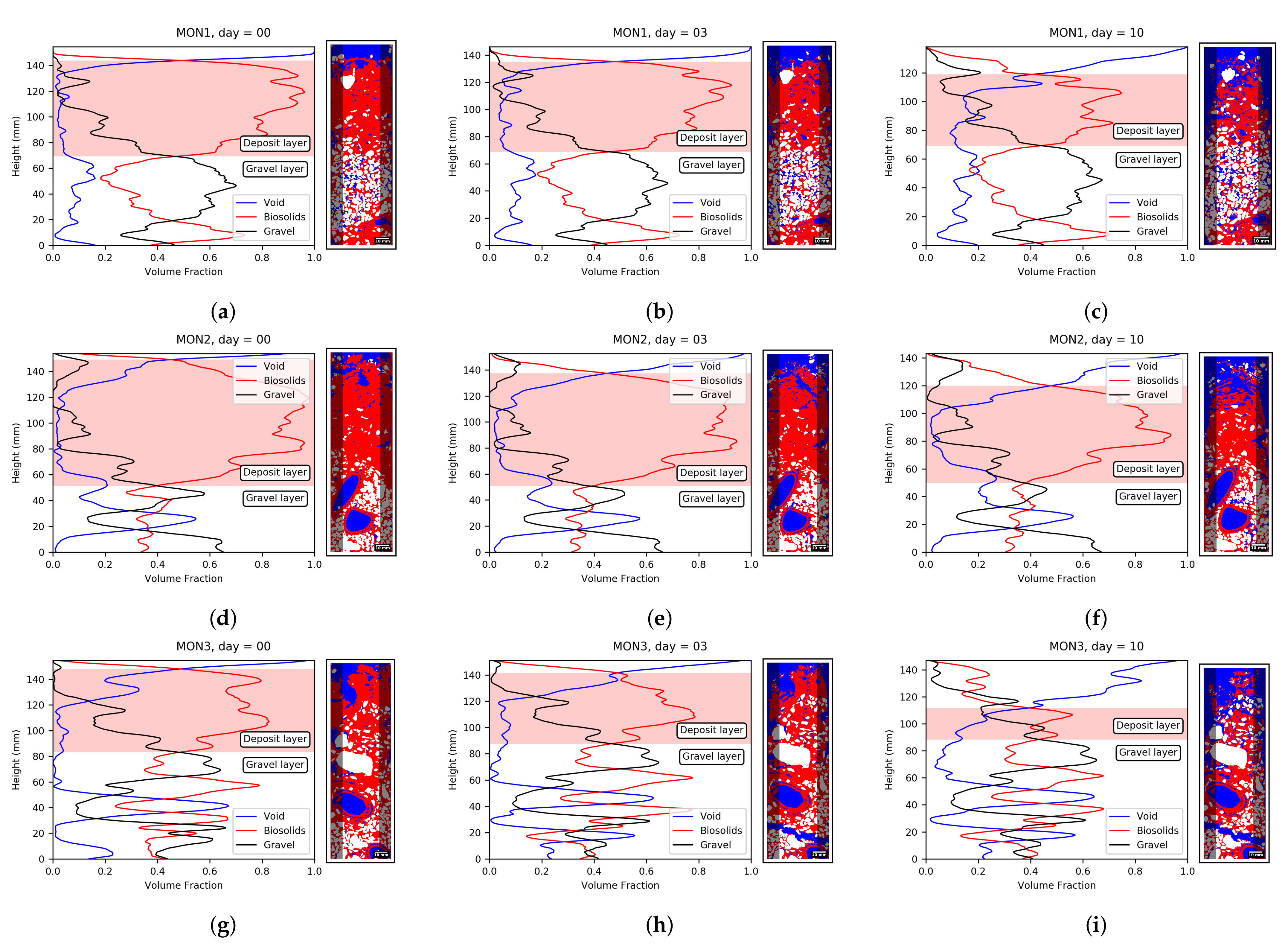
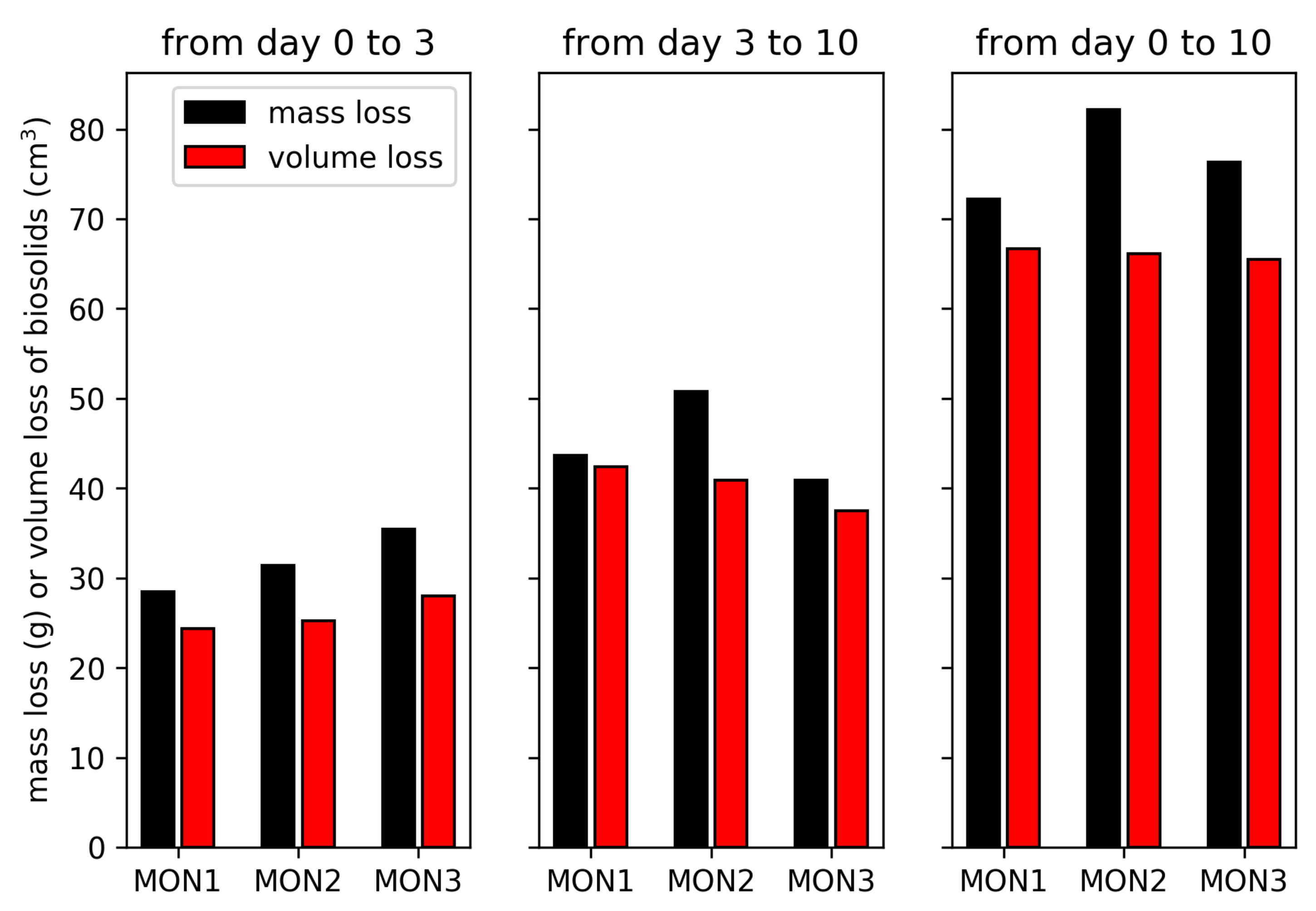
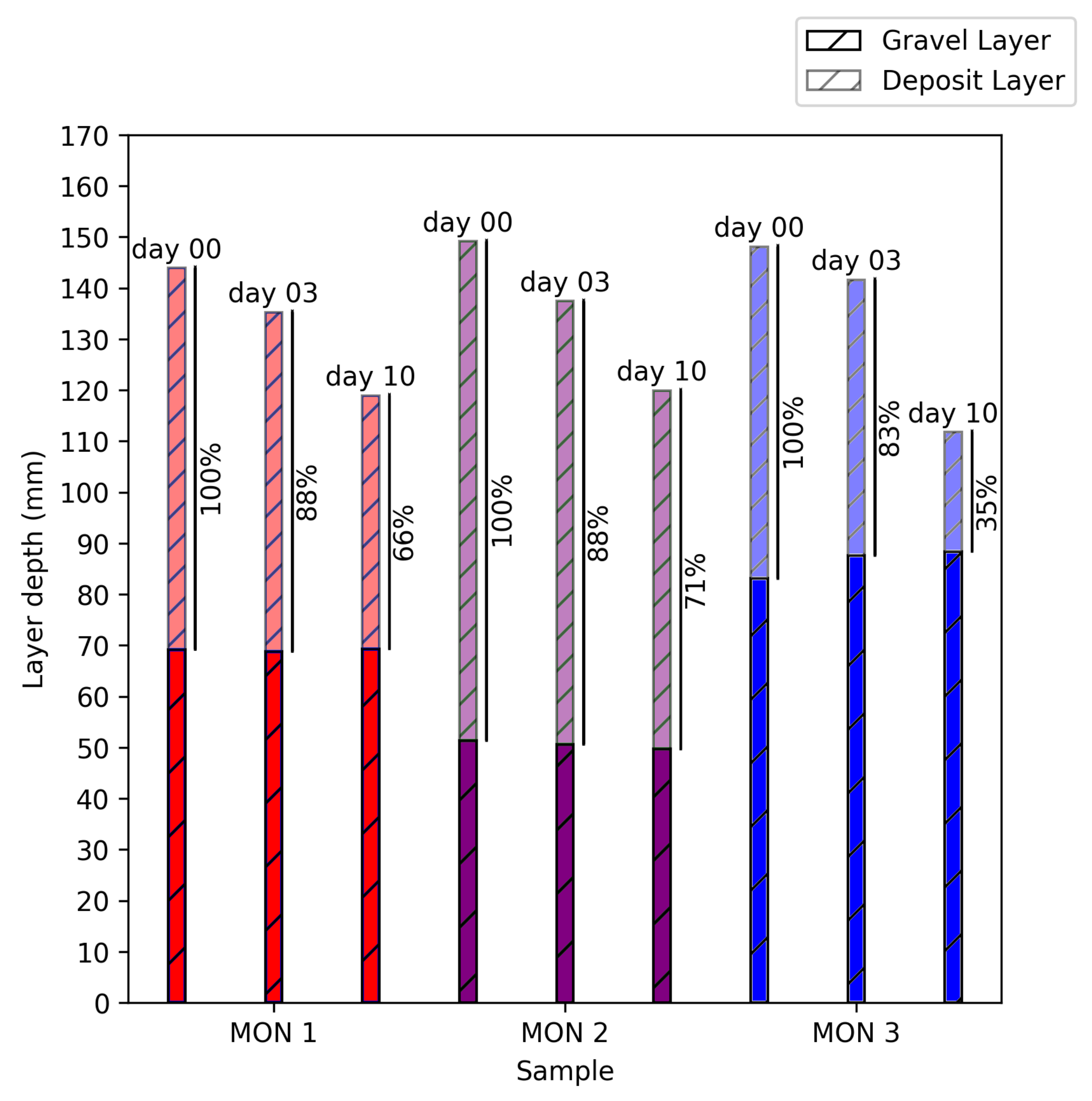
This study has demonstrated the applicability of X-ray CT to study structural changes in French VF treatment wetlands at the pore scale during the rest period. An ex situ experiment was performed in a drying chamber in order to simulate a rest period for samples containing the deposit layer and gravel layer of a French VF treatment wetland. An average evaporation rate of 2 mm · day 1 was measured; this value is representative of the lowest observations in full-scale treatment wetlands. Under these conditions, drying has induced major changes in the volumetric distribution and morphology of the phases in the samples. At the end of the drying period, the volume of biosolids had been reduced to 58% of its initial value on average. Most of this biosolid volume reduction could be observed in the deposit layer.
This work has confirmed the applicability of X-ray CT to understand the dynamics of structural changes in biosolids and voids within samples from French VF treatment wetlands during an ex situ drying experiment. Clogging is essentially a geometric phenomenon influenced by physical and biological processes in these wetlands; hence, changes in the structure and distribution of biosolids are keys that need to be understood.
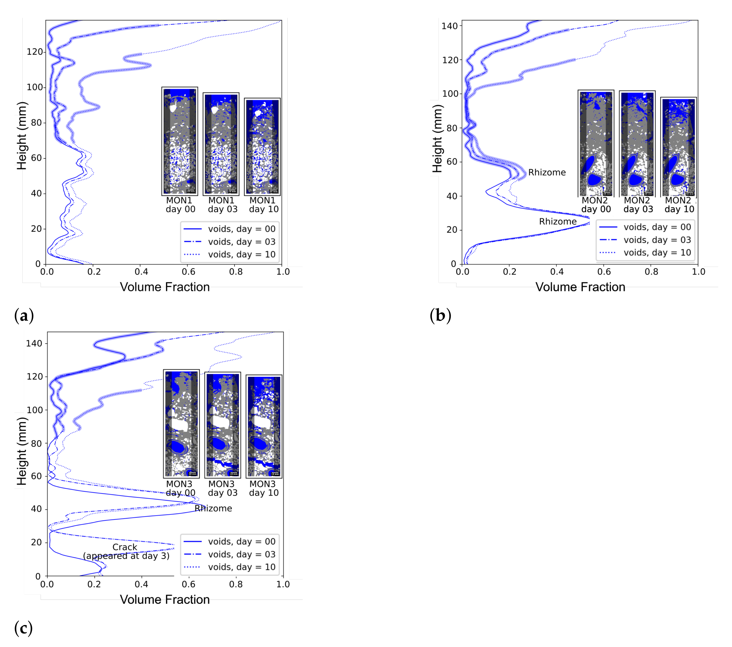
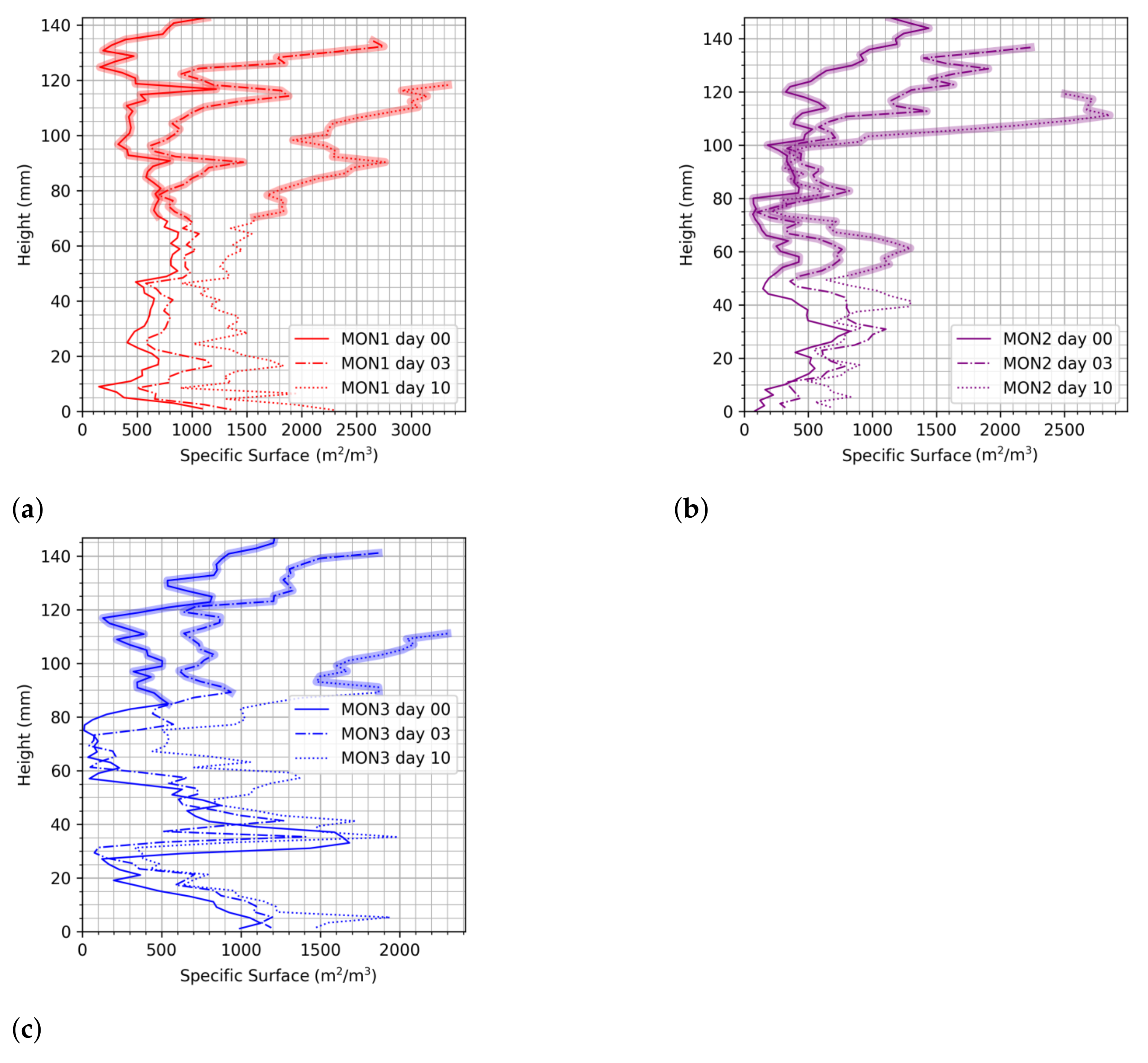
The reduction in biosolid volume fraction was 6 times greater in the deposit layer than in the gravel layer; moreover, the deposit layer thickness was reduced to 68% of its initial value. PSD evolved differently during the rest period depending on the given layer. The deposit layer showed an increase in void volume with sizes greater than 4 mm, as a result of radial shrinkage and crack development. When excluding the border effect, a void volume increase with sizes between 0 to 3 mm resulted from drying at the center of the sample. In the gravel layer, the void volume increase was mainly due to an increase in the pores ranging from 0 to 2 mm. The void/biosolid SSA rose from a minimum value of 1.1 to a maximum of 4.2 across the various samples. The SSA and its increase over time were also greater in the deposit layer. The connectivity of the void phase to the atmosphere increased from 19% at the beginning to 91% at the end of the experiment for just one of the samples.
The impact of the rest period on water flow in French VF treatment wetlands has already been discussed qualitatively and quantitatively, but only from a global approach with measurements, like infiltration rates. Nevertheless, the quantification of phenomena at the origin of changes in infiltration rate during the rest period, at the pore scale, has been lacking in the treatment wetland field, yet could be enabled by X-ray CT. Through these measurements, it has been confirmed that nearly all the biosolid structural changes contribute to increasing of the water permeability for the subsequent feeding period, namely: (1) a reduction in the deposit layer thickness, and increases in the (2) void volume, (3) pore size, and (4) connectivity.
By coupling gravimetric measurements with volumetric measurements, the biosolid phase structure can be described beyond the limits of X-ray CT resolution. The air-filled microporosity is another key physical variable to better understand the dynamics of mineralization and clogging, since it controls the oxygen transfer rate within the biosolids and their biological degradation. Based on a hypothesis of the behavior of water/organic matter mixtures, it was possible to estimate an average increase of 0.11 in the air-filled microporosity within the biosolid phase during the drying experiment.
This study demonstrates the suitability of X-ray tomography to measure relevant information of morphological changes in the porous structure of VFTW. These results can notably used to adjust the inlet parameters (porosity, pore size, thickness of the deposit layer) of the numerical models in use to simulate the operation of VFTW. By including the breakthroughs presented in this paper, models may achieve a better mechanistic description of the operation of TW. In order to study the influence of other parameters, like meteorological parameters (air temperature and humidity and wind speed), the methodology introduced in this study could be adapted to perform in situ surveys, notably to study seasonal effects on drying during the rest period. The influence of the changes in the microporous structure on oxygen transport could also be studied to imporve our understanding of the mechanisms that control the rate of aerobic biodegradation of biosolids, which is crucial in delaying the clogging of VFTW.

Author Contributions

Conceptualization, G.D.M.-C., L.O., P.M. and N.F.; methodology, G.D.M.-C., L.O. and N.F.; software, G.D.M.-C.; validation, G.D.M.-C. and N.F.; formal analysis, G.D.M.-C., L.O. and N.F.; investigation, G.D.M.-C., J.A. and N.F.; resources, J.A. and N.F.; data curation, G.D.M.-C. and J.A.; writing—original draft preparation, G.D.M.-C.; writing—review and editing, L.O. and N.F.; visualization, G.D.M.-C.; supervision, P.M.; project administration, P.M. and N.F.; funding acquisition, P.M. and N.F. All authors have read and agreed to the published version of the manuscript.

Funding

This research received no external funding.

Acknowledgments

We acknowledge Jérémie Aubert, Loïc Richard and Matthieu Masson for their technical support.

Conflicts of Interest

The authors declare no conflict of interest.

Abbreviations

The following abbreviations are used in this manuscript:
VFVertical flow
CTComputed tomography
p.e.People equivalent
SSSuspended solids
OMOrganic Matter
SSASpecific surface area
DNADeoxyribonucleic acid
FDEMFrequency domain electromagnetic method
PMMAPoly(methyl methacrylate)
VSSVolatile suspended solids
PVEPartial volume effect
PSDPore size distribution
ROIRegion of interest

Appendix A. Drying Condition Monitoring

Table A1. Mean and percentiles of the temperature and relative humidity in the drying chamber during drying.
Temperature (°C) Relative Humidity (%)
15th percentileMedian85th percentile15th percentileMedian85th percentile
27.027.427.633.248.154.8

Appendix B. Relative Sample Composition

Table A2. Composition of biosolids on Day 0.
VariableUnitSample 1Sample 2Sample 3
Waterg/g78.4%79.8 %79.9%
Volatile solids (VSS)g/g11.8%10.8%11.2%
Ashesg/g9.8%9.4 %8.9%

Appendix C. Average Volume Fractions

Table A3. Average volume fractions of voids and biosolids, plus gravel in both the deposit layer and gravel layer. Computations were performed for a ROI of 60%.
Volume Fraction Volume Fraction Volume Fraction
SampleLayerPhaseDay 0Day 3Day 10PhaseDay 0Day 3Day 10PhaseDay 0Day 3Day 10
MON1DepositVoid0.050.080.19Biosolids0.810.760.61Gravel0.140.160.20
MON1GravelVoid0.090.110.14Biosolids0.380.370.34Gravel0.530.520.52
MON2DepositVoid0.090.110.13Biosolids0.790.770.71Gravel0.120.120.16
MON2GravelVoid0.220.240.25Biosolids0.370.350.35Gravel0.410.410.40
MON3DepositVoid0.130.170.19Biosolids0.700.630.48Gravel0.170.200.33
MON3GravelVoid0.150.190.22Biosolids0.460.440.41Gravel0.390.370.37

Appendix D. Evolution of the Deposit and Gravel Layer Thicknesses

Figure A1. Evolution of deposit and gravel layer thicknesses during the drying experiment: computations were performed for an ROI of 60%.
Water 13 00389 g0a1

Appendix E. Average SSA Values

Table A4. Average SSA for the deposit and gravel layers and increase over time. Computations were performed for an ROI of 60%.
Average SSA in m 1 (SSA Day i)/(SSA Day 0)
SampleDayiDeposit LayerGravel LayerDeposit LayerGravel Layer
1055263711
312028442.21.3
10234013754.22.2
2050141011
38336601.71.6
1010817992.21.9
3057354911
39815971.71.1
1018329943.21.8

References

  1. Morvannou, A.; Forquet, N.; Michel, S.; Troesch, S.; Molle, P. Treatment Performances of French Constructed Wetlands: Results from a Database Collected over the Last 30 Years. Water Sci. Technol. 2015, 71, 1333–1339. [Google Scholar] [CrossRef] [PubMed] [Green Version]
  2. Molle, P. French Vertical Flow Constructed Wetlands: A Need of a Better Understanding of the Role of the Deposit Layer. Water Sci. Technol. 2014, 69, 106–112. [Google Scholar] [CrossRef] [PubMed]
  3. Herzig, J.P.; Leclerc, D.M.; Goff, P.L. Flow of Suspensions through Porous Media—Application to Deep Filtration. Ind. Eng. Chem. 1970, 62, 8–35. [Google Scholar] [CrossRef]
  4. Molle, P.; Liénard, A.; Boutin, C.; Merlin, G.; Iwema, A. How to Treat Raw Sewage with Constructed Wetlands: An Overview of the French Systems. Water Sci. Technol. 2005, 51, 11–21. [Google Scholar] [CrossRef] [PubMed]
  5. Pucher, B.; Langergraber, G. The State of the Art of Clogging in Vertical Flow Wetlands. Water 2019, 11, 2400. [Google Scholar] [CrossRef] [Green Version]
  6. Kania, M.; Gautier, M.; Michel, P.; Gourdon, R. Study of Aggregation in Surface Sludge Deposits from 14 Full-Scale French Constructed Wetlands Using Particle Size Distribution and Dynamic Vapor Sorption Analyses. Water Sci. Technol. 2018, 77, 79–90. [Google Scholar] [CrossRef]
  7. Liénard, A. Vertical Flow Constructed Wetlands Fed with Raw Sewage: Historical Review and Recent Developments in France. In Proceedings of the 12th International Conference on Wetland Systems for Water Pollution Control, Venice, Italy, 4–9 October 2010. [Google Scholar]
  8. Nivala, J.; Knowles, P.; Dotro, G.; García, J.; Wallace, S. Clogging in Subsurface-Flow Treatment Wetlands: Measurement, Modeling and Management. Water Res. 2012, 46, 1625–1640. [Google Scholar] [CrossRef]
  9. Breul, P.; Gourves, R. In Field Soil Characterization: Approach Based on Texture Image Analysis. J. Geotech. Geoenviron. Eng. 2006, 132, 102–107. [Google Scholar] [CrossRef]
  10. Kim, B.; Forquet, N. Pore-Scale Observation of Deposit within the Gravel Matrix of a Vertical Flow Constructed Wetland. Environ. Technol. 2016, 37, 3146–3150. [Google Scholar] [CrossRef] [Green Version]
  11. Martinez-Carvajal, G.D.; Oxarango, L.; Adrien, J.; Molle, P.; Forquet, N. Assessment of X-Ray Computed Tomography to Characterize Filtering Media from Vertical Flow Treatment Wetlands at the Pore Scale. Sci. Total. Environ. 2019, 658, 178–188. [Google Scholar] [CrossRef]
  12. MacLeod, G.; Adderley, P.; Simpson, I.; Wilson, C. Thin Section & Micromorphology. Available online: http://www.thin.stir.ac.uk/ (accessed on 1 February 2018).
  13. Martinez-Carvajal, G.D.; Oxarango, L.; Clément, R.; Molle, P.; Forquet, N. Assessment of Spatial Representativity of X-Ray Tomography to Study Vertical Flow Treatment Wetlands. Sci. Total. Environ. 2020, 713, 136510. [Google Scholar] [CrossRef] [PubMed]
  14. Wildenschild, D.; Sheppard, A.P. X-Ray Imaging and Analysis Techniques for Quantifying Pore-Scale Structure and Processes in Subsurface Porous Medium Systems. Adv. Water Resour. 2013, 51, 217–246. [Google Scholar] [CrossRef]
  15. Leonard, A.; Blacher, S.; Marchot, P.; Pirard, J.P.; Crine, M. Image Analysis of X-Ray Microtomograms of Soft Materials during Convective Drying. J. Microsc. 2003, 212, 197–204. [Google Scholar] [CrossRef] [PubMed] [Green Version]
  16. Leonard, A.; Blacher, S.; Marchot, P.; Crine, M. Use of X-Ray Microtomography to Follow the Convective Heat Drying of Wastewater Sludges. Dry. Technol. 2002, 20, 1053–1069. [Google Scholar] [CrossRef] [Green Version]
  17. Léonard, A.; Blacher, S.; Marchot, P.; Pirard, J.P.; Crine, M. Moisture Profiles Determination During Convective Drying Using X-Ray Microtomography. Can. J. Chem. Eng. 2005, 83, 127–131. [Google Scholar] [CrossRef] [Green Version]
  18. Mathews, J.P.; Pone, J.D.N.; Mitchell, G.D.; Halleck, P. High-Resolution X-Ray Computed Tomography Observations of the Thermal Drying of Lump-Sized Subbituminous Coal. Fuel Process. Technol. 2011, 92, 58–64. [Google Scholar] [CrossRef]
  19. Rezanezhad, F.; Quinton, W.L.; Price, J.S.; Elrick, D.; Elliot, T.R.; Heck, R.J. Examining the Effect of Pore Size Distribution and Shape on Flow through Unsaturated Peat Using 3-D Computed Tomography. Hydrol. Earth Syst. Sci. Discuss. 2009, 6, 3835–3862. [Google Scholar] [CrossRef]
  20. Aminnaji, M.; Rabbani, A.; Niasar, V.J.; Babaei, M. Effects of Pore-Scale Heterogeneity on Macroscopic NAPL Dissolution Efficiency: A Two-Scale Numerical Simulation Study. Water Resour. Res. 2019, 55, 8779–8799. [Google Scholar] [CrossRef] [Green Version]
  21. Al-Raoush, R.; Papadopoulos, A. Representative Elementary Volume Analysis of Porous Media Using X-Ray Computed Tomography. Powder Technol. 2010, 200, 69–77. [Google Scholar] [CrossRef]
  22. Costanza-Robinson, M.S.; Estabrook, B.D.; Fouhey, D.F. Representative Elementary Volume Estimation for Porosity, Moisture Saturation, and Air-Water Interfacial Areas in Unsaturated Porous Media: Data Quality Implications. Water Resour. Res. 2011, 47, 1–12. [Google Scholar] [CrossRef]
  23. Zhang, D.; Zhang, R.; Chen, S.; Soll, W.E. Pore Scale Study of Flow in Porous Media: Scale Dependency, REV, and Statistical REV. Geophys. Res. Lett. 2000, 27, 1195–1198. [Google Scholar] [CrossRef]
  24. Feldkamp, L.A.; Davis, L.C.; Kress, J.W. Practical Cone-Beam Algorithm. JOSA A 1984, 1, 612–619. [Google Scholar] [CrossRef] [Green Version]
  25. Schindelin, J.; Arganda-Carreras, I.; Frise, E.; Kaynig, V.; Longair, M.; Pietzsch, T.; Preibisch, S.; Rueden, C.; Saalfeld, S.; Schmid, B.; et al. Fiji: An Open-Source Platform for Biological-Image Analysis. Nat. Methods 2012, 9, 676–682. [Google Scholar] [CrossRef] [PubMed] [Green Version]
  26. Bhattad, P.; Willson, C.S.; Thompson, K.E. Segmentation of Low-Contrast Three-Phase X-Ray Computed Tomography Images of Porous Media. In Advances in Computed Tomography for Geomaterials; John Wiley & Sons, Ltd.: London, UK, 2013; pp. 254–261. [Google Scholar] [CrossRef]
  27. Pilny, V.; Janacek, J. Anisotropic Diffusion 2D. 2006. Available online: https://imagej.net/AnisotropicDiffusion2D (accessed on 1 February 2021).
  28. Tschumperlé, D.; Deriche, R. Vector-Valued Image Regularization with PDE’s: A Common Framework for Different Applications. In CVPR’03, Proceedings of the 2003 IEEE Computer Society Conference on Computer Vision and Pattern Recognition; IEEE Computer Society: Washington, DC, USA, 2003; pp. 651–656. [Google Scholar]
  29. Hashemi, M.A.; Khaddour, G.; François, B.; Massart, T.J.; Salager, S. A Tomographic Imagery Segmentation Methodology for Three-Phase Geomaterials Based on Simultaneous Region Growing. Acta Geotech. 2014, 9, 831–846. [Google Scholar] [CrossRef]
  30. Lehmann, G.; Legland, D. Efficient N-Dimensional Surface Estimation Using Crofton Formula and Run-Length Encoding. Insight J. 2012, 2, 1–11. [Google Scholar]
  31. Legland, D.; Kiêu, K.; Devaux, M.F. Computation of Minkowski Measures on 2D and 3D Binary Images. Image Anal. Stereol. 2011, 26, 83. [Google Scholar] [CrossRef] [Green Version]
  32. Santaló, L.A. Integral Geometry and Geometric Probability, 2nd ed.; Cambridge University Press: Cambridge, UK, 2004. [Google Scholar] [CrossRef]
  33. Dougherty, B.; Schindelin, J.; Doube, M.; Domander, R.; Hiner, M.; Rueden, C.; Coeurjolly, D.; Kunzelmann, K.H. Local Thickness. 2017. Available online: https://imagej.net/Local_Thickness (accessed on 1 February 2021).
  34. Hildebrand, T.; Rüegsegger, P. A New Method for the Model-Independent Assessment of Thickness in Three-Dimensional Images. J. Microsc. 1997, 185, 67–75. [Google Scholar] [CrossRef]
  35. Saito, T.; Toriwaki, J.I. New Algorithms for Euclidean Distance Transformation of an N-Dimensional Digitized Picture with Applications. Pattern Recognit. 1994, 27, 1551–1565. [Google Scholar] [CrossRef]
  36. Chang, C.; Zhou, Q.; Kneafsey, T.J.; Oostrom, M.; Wietsma, T.W.; Yu, Q. Pore-Scale Supercritical CO2 Dissolution and Mass Transfer under Imbibition Conditions. Adv. Water Resour. 2016, 92, 142–158. [Google Scholar] [CrossRef] [Green Version]
  37. Taniguchi, N.; Fujibayashi, S.; Takemoto, M.; Sasaki, K.; Otsuki, B.; Nakamura, T.; Matsushita, T.; Kokubo, T.; Matsuda, S. Effect of Pore Size on Bone Ingrowth into Porous Titanium Implants Fabricated by Additive Manufacturing: An in Vivo Experiment. Mater. Sci. Eng. C 2016, 59, 690–701. [Google Scholar] [CrossRef] [Green Version]
  38. Mickel, W.; Munster, S.; Jawerth, L.M.; Vader, D.A.; Weitz, D.A.; Sheppard, A.P.; Mecke, K.; Fabry, B.; Schroder-Turk, G.E. Robust Pore Size Analysis of Filamentous Networks from Three-Dimensional Confocal Microscopy. Biophys. J. 2008, 95, 6072–6080. [Google Scholar] [CrossRef] [PubMed] [Green Version]
  39. Ruiz, T.; Wisniewski, C. Correlation between Dewatering and Hydro-Textural Characteristics of Sewage Sludge during Drying. Sep. Purif. Technol. 2008, 61, 204–210. [Google Scholar] [CrossRef]
  40. Masmoudi, W.; Prat, M. Heat and Mass Transfer between a Porous Medium and a Parallel External Flow. Application to Drying of Capillary Porous Materials. Int. J. Heat Mass Transf. 1991, 34, 1975–1989. [Google Scholar] [CrossRef]
  41. Vincent, J. Les Lits de Séchage de Boue Plantés de Roseaux Pour Le Traitement Des Boues Activées et Les Matières de Vidange: Adapter La Stratégie de Gestion Pour Optimiser Les Performances. Ph.D Thesis, Université Montpellier 2, Montpellier, France, 2011. [Google Scholar]
  42. Hua, G.; Zeng, Y.; Zhao, Z.; Cheng, K.; Chen, G. Applying a Resting Operation to Alleviate Bioclogging in Vertical Flow Constructed Wetlands: An Experimental Lab Evaluation. J. Environ. Manag. 2014, 136, 47–53. [Google Scholar] [CrossRef]
  43. Knowles, P.; Dotro, G.; Nivala, J.; García, J. Clogging in Subsurface-Flow Treatment Wetlands: Occurrence and Contributing Factors. Ecol. Eng. 2011, 37, 99–112. [Google Scholar] [CrossRef]
  44. Sun, X.; Dai, Q.; Ng, K. Computational Investigation of Pore Permeability and Connectivity from Transmission X-Ray Microscope Images of a Cement Paste Specimen. Constr. Build. Mater. 2014, 68, 240–251. [Google Scholar] [CrossRef]
  45. Bhattad, P.; Willson, C.S.; Thompson, K.E. Effect of Network Structure on Characterization and Flow Modeling Using X-Ray Micro-Tomography Images of Granular and Fibrous Porous Media. Transp. Porous Media 2011, 90, 363. [Google Scholar] [CrossRef]
Figure 1. A sketch of the drying chamber.
Water 13 00389 g001
Figure 2. Mass changes vs. time (left), cumulative mass losses (top right) and evaporation rates (bottom right) during the experiment.
Water 13 00389 g002
Figure 3. Horizontal slices in the deposit layer (ac) and in the gravel layer (df) for MON1 sample. (a) MON1, deposit layer (day 0, height = 116 mm), (b) MON1, deposit layer (day 3, height = 115 mm), (c) MON1, deposit layer (day 10, height = 112 mm), (d) MON1, gravel layer (day 0, height = 33 mm), (e) MON1, gravel layer (day 3, height = 33 mm), (f) MON1, gravel layer (day 10, height = 33 mm).
Water 13 00389 g003
Figure 4. Evolution of vertical phase volume fraction profiles and snapshot on a vertical slice of the 3D scan. Computation were performed for a ROI of 60%. (a) MON1, day 0, (b) MON1, day 3, (c) MON1, day 10, (d) MON2, day 0, (e) MON2, day 3, (f) MON2, day 10, (g) MON3, day 0, (h) MON3, day 3, (i) MON3, day 10.
Water 13 00389 g004
Figure 5. Evolution of the void phase volume fraction profiles. The deposit layer is represented by a wider trace in the curves. Computations were performed for a region of interest (ROI) of 60%. (a) MON1, (b) MON2, (c) MON3.
Water 13 00389 g005
Figure 6. Cumulative Pore Size Distributions (PSD) associated to snapshots highlighting the ROI on which computation are performed (on the right). (a) MON1, gravel layer, (b) MON1, deposit layer ROI = 100%, (c) MON1, deposit layer ROI = 60%, (d) MON2, gravel layer, (e) MON2, deposit layer ROI = 100%, (f) MON 2, deposit layer ROI = 60%, (g) MON3, gravel layer, (h) MON3, deposit layer ROI = 100%, (i) MON3, deposit layer ROI = 60%.
Water 13 00389 g006
Figure 7. Specific Surface Areas (SSA) profiles. The deposit layer is represented by a wider trace in the curves. Computations were performed for a ROI of 60%. (a) MON1, (b) MON2, (c) MON3.
Water 13 00389 g007
Figure 8. Cumulative void phase connectivity profiles: computations were performed for an ROI of 60%.
Water 13 00389 g008
Figure 9. Comparison of mass and volume losses.
Water 13 00389 g009
Table 1. Sample composition.
VariableUnitSample 1Sample 2Sample 3
Total water (at day 0)g138.77166.72142.74
Mass of volatile solids (VSS)g20.9722.6119.95
Mass of ashesg17.2619.7115.93
Mass of gravelg203.77154.41187.73
Total water mass fraction (at day 0)g/g36.4%45.9%39.0%
Volatile solid mass fraction (VSS)g/g5.5%6.2%5.4%
Ash mass fractiong/g4.5%5.4%4.3%
Gravel mass fractiong/g53.5%42.5%51.2%
Table 2. Volumes of various phases over the entire sample.
Volume (cm 3 )
PhaseSampleDay 0Day 3Day 10
1817980
Gravel2616059
3727171
114812381
Biosolids2178153112
315012285
14572113
Void23460101
35282119
Table 3. Increase in the air-filled microporosity volume fraction ( Δ θ m i c r o p o r o s i t y ).
MON1MON2MON3
Day 30.030.040.06
Day 100.070.140.13
Publisher’s Note: MDPI stays neutral with regard to jurisdictional claims in published maps and institutional affiliations.

