Probabilistic Characterization of the Vegetated Hydrodynamic System Using Non-Parametric Bayesian Networks ^†

Abstract

The increasing risk of flooding requires obtaining generalized knowledge for the implementation of distinct and innovative intervention strategies, such as nature-based solutions. Inclusion of ecosystems in flood risk management has proven to be an adaptive strategy that achieves multiple benefits. However, obtaining generalizable quantitative information to increase the reliability of such interventions through experiments or numerical models can be expensive, laborious, or computationally demanding. This paper presents a probabilistic model that represents interconnected elements of vegetated hydrodynamic systems using a nonparametric Bayesian network (NPBN) for seagrasses, salt marshes, and mangroves. NPBNs allow for a system-level probabilistic description of vegetated hydrodynamic systems, generate physically realistic varied boundary conditions for physical or numerical modeling, provide missing information in data-scarce environments, and reduce the amount of numerical simulations required to obtain generalized results—all of which are critically useful to pave the way for successful implementation of nature-based solutions.

1. Introduction

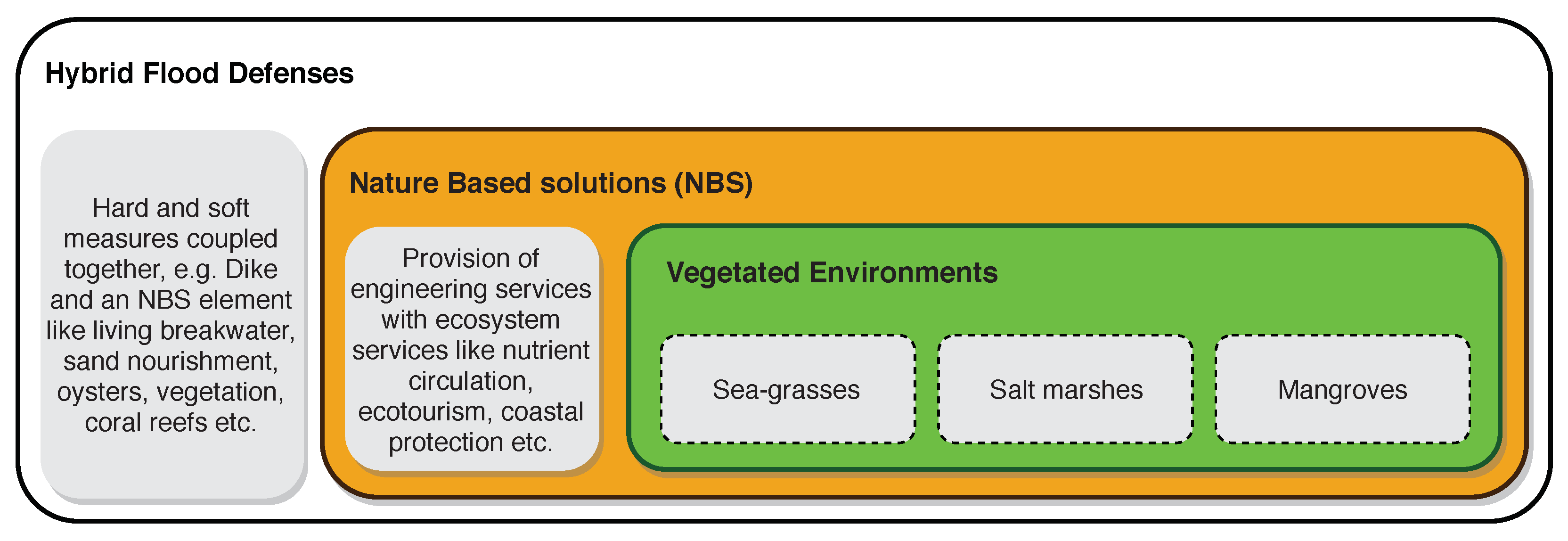
Coastal flood risk is an alarming threat due to increasing hazard and vulnerability as a consequence of climatic and anthropogenic changes [1]. To counter that, protection measures combining conventional and nature-based solutions can constitute robust hybrid defense systems for risk mitigation [2,3,4]. Moreover, vegetation as a nature-based solution for flood defense, under the umbrella of hybrid solutions (see Figure 1), has shown convincing potential for flood hazard (wave load) reduction [5,6,7,8,9,10,11,12,13,14,15,16]. Several studies look at vegetation and reduction of currents and waves through numerical modeling [12,15,17,18,19] or experiments [9,11,14,20], see Table 1. However, combined designs with vegetation and conventional defenses that are implemented in the field are scarce.

Despite many studies focused on hydraulic load reduction by vegetation, there is no general consensus or coherent set of guidelines yet that enable uniform integration of vegetated coastal ecosystems in design for vegetation-levee combinations. This maybe due to the varying estimates of wave attenuation resulting from the case studies. For instance, in Table 1, a few flume and field experimental studies have been synthesized showing a variety of hydrodynamic and vegetation characteristics that were tested to determine drag coefficient expressions. It can be observed that the resulting drag coefficient expressions are considerably different and yield distinct values for the same Reynolds number, see [13]. Since the drag coefficient is a critical variable for the calibration of numerical models, estimates of wave attenuation potential of vegetation also differ considerably, which undermines the reliability of vegetation as an integrated element of a flood defense systems.

Instead of case-specific varying point estimates, a wide range of results in multiple biohydrophysical conditions are required which could be generalized to develop the implementation guidelines for nature-based solutions. However, not only the generalized results are missing but the boundary conditions required to measure or model those results are also missing. A potential reason could be the lack of holistic system-level description of vegetated hydrodynamic systems which means that the vegetated foreshores have not been quantified as a system with interacting and correlated constituting elements. Therefore, this study provides a first attempt to develop a probabilistic model of vegetated hydrodynamic system which would help in obtaining the necessary boundary conditions to describe and numerically model the system for a variety of situations more efficiently. We synthesize prior studies parameterizing individual variables in the system [21,22,23,24,25,26,27,28,29] and build on that to study complete system dynamics and its response to variations.

Table 1. Review of experimental work presenting variety of hydrodynamic and vegetation properties. See nomenclature for variables’ explanation. Inspired from [13,30,31,32,33].

Study	Hydrodynamic Properties	Vegetation Characteristics	Drag Coefficient
Flume [34]	Regular waves $h=0.50$ m $H_{m0}$ = 0.036–0.19 m	Polypropylene strips as artificial kelp $h_v=0.25$ m, 52 × 0.03 mm, $N_v$ = 1110–1490 m${}^{-2}$	–
Flume [6]	Used [34]	Used [34]	$C_d=0.08+{\left(\frac{2200}{R_e}\right)}^{2.4}$ $2200<R_e<18000$
Flume [35]	Used [34]	Used [34] and distinguished for rigid and flexible vegetation	Rigid $C_d=0.08+{\left(\frac{2200}{R_e}\right)}^{2.2}$ $200<R_e<15500$ Flex. $C_d=0.40+{\left(\frac{4600}{R_e}\right)}^{2.9}$ $2300<R_e<22000$
Flume [36]	Regular waves h = 0.4–1.0 m $H_{m0}$ = 0.045–0.17 m	L. hyperborea $h_v=0.20$ m, $b_v=25$ mm, $N_v=1200$ m${}^{-2}$	$C_d=0.47exp(-0.052KC)$ $3<KC<59$
Field (seagrass) [37]	Irregular waves h = 1–1.5 m $H_{m0}\approx 0.09$ m	Thalassia testundinum $h_v$ = 0.25–0.30 m, $b_v=0.33$ mm, $N_v=1100$ m${}^{-2}$ (Used relative velocity for drag calculation)	$C_d=0.10+{\left(\frac{925}{R_e}\right)}^{-3.16}$ $200<R_e<800$ $C_d=126.45{KC}^{-2.7}$ $0<KC<6$
Flume [8]	Both Regular & Irregular h = 0.3–0.8 m $H_{m0}$ = 0.05–0.13 m (Reg.) $H_{m0}$ = 0.03–0.13 m (Irreg.)	Posidonia oceanica $h_v=0.1$ m, $b_v=3$ mm, $N_v=40000$ m${}^{-2}$	$C_d=22.9{KC}^{-1.09}$ $15<KC<425$
Field (seagrass) [7]	Irregular waves $h\approx$ 0.75–3.5 m $H_{m0}\approx$0.05–0.18 m	Zostera noltii $h_v=0.13\pm 0.030$ m, $N_{v,avg}=625\pm 225$ m${}^{-2}$	$C_d=0.06+{\left(\frac{153}{R_e}\right)}^{1.45}$ $100<R_e<1000$
Field (Salt marsh) [38]	Irregular waves $h\approx 0.55$ m $H_{m0}=<0.4$ m	Spartina alterniflora $h_v\approx 0.63$ m, $b_v\approx 8$ mm, $N_v\approx 422$ m${}^{-2}$	$C_d=0.36+{\left(\frac{2600}{R_e}\right)}^{1.0}$ $600<R_e<3200$
Field (Seagrass) [39]	Irregular waves (Storms) h = 6.5–16.5 m $H_{m0}$ = 0.10–1.31 m	Posidonia oceanica $h_v=0.8\pm 0.1$ m, $b_v\approx 4$ mm, $N_v=615\pm 34$ m${}^{-2}$	Used [8]
Field (Salt marsh) [40]	Irregular waves h = 0.4–0.82 m $H_{m0}$ = 0.15–0.4 m	Spartina alterniflora $h_v\approx 0.22$ m, $b_v\approx 8$ mm, $N_v\approx 422$ m${}^{-2}$	$C_d=70{KC}^{-0.86}$ $25<KC<135$
Statistical [41]	Statistical evaluation of 35 studies	Statistical evaluation of kelp, seagrass, saltmarsh and mangroves	${log}_{10}\left({\mathbf{C}}_{\mathbf{d},ijk}\right)={\beta }_0+{\beta }_{1}log(\mathrm{c}·R_e)+\delta$ $17000<R_e<350000$
Flume [42] Rigid Flexible	Regular waves h = 1.8–2.4 m $H_{m0}$ = 0.4–0.5 m h = 0.4–1.0 m $H_{m0}$ = 0.045–0.17 m	Posidonia oceanica (Polypropylene) $h_v=0.35,0.55$ m, $b_v=1$ mm, $N_v=360,180$ m${}^{-2}$ Artificial seagrass (PVC strips) $h_v=0.27,0.45$ m, $b_v=1$ mm, $N_v=360,180$ m${}^{-2}$	$C_d=0.87+{\left(\frac{2200}{R_e}\right)}^{0.88}$ $C_d=1.61+{\left(\frac{4600}{R_e}\right)}^{1.9}$ $1000<R_e<3500$
Flume [43] Rigid Flexible	Regular waves h = 0.4–0.7 m $H_{m0}$ = 0.03–0.15 m Irregular waves h = 0.5–0.7 m $H_{m0}$ = 0.03–0.10 m	Wooden cylinders (Rigid) $h_v$ = 0.48, 0.63 m, $b_v=9.4$ mm, $N_v=156,350,623$ m${}^{-2}$ Spartina alterniflora (Flexible) $h_v=0.59\pm 0.21$ m, $b_v=6.5\pm 0.9$ mm, $N_v=405$ m${}^{-2}$ Juncus roemerianus (Flexible) $h_v=1.03\pm 0.27$ m, $b_v=2.4\pm 0.6$ mm, $N_v=2857$ m${}^{-2}$	Rigid $C_d=2.1+{\left(\frac{793}{R_e}\right)}^{2.39}$ $200<R_e<4500$ $C_d=1.5+{\left(\frac{6.785}{KC}\right)}^{2.22}$ $5<KC<100$ Flexible $C_d=0.683+{\left(\frac{12.07}{KC}\right)}^{2.25}$ $5<KC<350$
Flume [44]	Irregular waves h = 0.31–0.53 m $H_{m0}$ = 0.05–0.19 m	Spartina alterniflora (Polyolefin tubes) $h_v$ = 0.41 m, $b_v=6.4$ mm, $N_v=200,400$ m${}^{-2}$	$C_d=0.76+{\left(\frac{744.2}{R_e}\right)}^{1.27}$ $553<R_e<2296$ $C_d=1.1{\left(\frac{27.4}{KC}\right)}^{3.08}$ $26<KC<112$
Flume [45]	Regular waves & currents $h=0.25,0.50$ m $H_{m0}$ = 0.04–0.20 m	Vegetation mimics (Wooden rods) $h_v=0.36$ m, $b_v=10$ mm, $N_v=62,139,556$ m${}^{-2}$	$C_d=1.04+{\left(\frac{730}{R_e}\right)}^{1.37}$ $300<R_e<4700$
Flume [11]	Irregular waves $h=2$ m $H_{m0}$ = 0.2–0.7 m	Puccinellia maritima $h_v=0.22\pm 0.03$ m, $b_v=1.1\pm 0.3$ mm Elymus athericus $h_v=0.7\pm 0.01$ m, $b_v=1.3\pm 0.3$ mm	$C_d=0.16+{\left(\frac{227.3}{R_e}\right)}^{1.615}$ $100<R_e<1100$
Flume [46]	Both Regular & Irregular waves & currents $h=0.4,0.6$ m $H_{m0}=0.15,0.2$ m (Regular) $H_{m0}=0.12$ m (Irregular) Current vel.$=0.30$ ms${}^{-1}$	Spartina anglica $h_v=0.284$ m, $b_v=6$ mm, $N_v=420,729$ m${}^{-2}$ Puccinellia maritima $h_v=0.473$ m, $b_v=3$ mm, $N_v=877,1389,2436$ m${}^{-2}$	Irregular waves $C_d=0.08+{\left(\frac{22000}{R_e}\right)}^{2.2}$ Irregular waves + current $C_d=0.25+{\left(\frac{35000}{R_e}\right)}^9$ Irregular waves − current $C_d=0.50+{\left(\frac{27000}{R_e}\right)}^9$ $25000<R_e<60000$
Flume (Mangroves) [17]	Both Regular & Irregular $h=0.65$ m $H_{m0}$ = 0.01–0.1 m Regular $H_{m0}$ = 0.03–0.15 m Irreg.	Wooden cylinders (Rigid mangroves) $h_v>0.75$ m, $b_v=12$ mm, $N_v=200,400$ m${}^{-2}$	Used $C_d=1.5$ from [45]

Table 1. Review of experimental work presenting variety of hydrodynamic and vegetation properties. See nomenclature for variables’ explanation. Inspired from [13,30,31,32,33].

Study	Hydrodynamic Properties	Vegetation Characteristics	Drag Coefficient
Flume [34]	Regular waves $h=0.50$ m $H_{m0}$ = 0.036–0.19 m	Polypropylene strips as artificial kelp $h_v=0.25$ m, 52 × 0.03 mm, $N_v$ = 1110–1490 m${}^{-2}$	–
Flume [6]	Used [34]	Used [34]	$C_d=0.08+{\left(\frac{2200}{R_e}\right)}^{2.4}$ $2200<R_e<18000$
Flume [35]	Used [34]	Used [34] and distinguished for rigid and flexible vegetation	Rigid $C_d=0.08+{\left(\frac{2200}{R_e}\right)}^{2.2}$ $200<R_e<15500$ Flex. $C_d=0.40+{\left(\frac{4600}{R_e}\right)}^{2.9}$ $2300<R_e<22000$
Flume [36]	Regular waves h = 0.4–1.0 m $H_{m0}$ = 0.045–0.17 m	L. hyperborea $h_v=0.20$ m, $b_v=25$ mm, $N_v=1200$ m${}^{-2}$	$C_d=0.47exp(-0.052KC)$ $3<KC<59$
Field (seagrass) [37]	Irregular waves h = 1–1.5 m $H_{m0}\approx 0.09$ m	Thalassia testundinum $h_v$ = 0.25–0.30 m, $b_v=0.33$ mm, $N_v=1100$ m${}^{-2}$ (Used relative velocity for drag calculation)	$C_d=0.10+{\left(\frac{925}{R_e}\right)}^{-3.16}$ $200<R_e<800$ $C_d=126.45{KC}^{-2.7}$ $0<KC<6$
Flume [8]	Both Regular & Irregular h = 0.3–0.8 m $H_{m0}$ = 0.05–0.13 m (Reg.) $H_{m0}$ = 0.03–0.13 m (Irreg.)	Posidonia oceanica $h_v=0.1$ m, $b_v=3$ mm, $N_v=40000$ m${}^{-2}$	$C_d=22.9{KC}^{-1.09}$ $15<KC<425$
Field (seagrass) [7]	Irregular waves $h\approx$ 0.75–3.5 m $H_{m0}\approx$0.05–0.18 m	Zostera noltii $h_v=0.13\pm 0.030$ m, $N_{v,avg}=625\pm 225$ m${}^{-2}$	$C_d=0.06+{\left(\frac{153}{R_e}\right)}^{1.45}$ $100<R_e<1000$
Field (Salt marsh) [38]	Irregular waves $h\approx 0.55$ m $H_{m0}=<0.4$ m	Spartina alterniflora $h_v\approx 0.63$ m, $b_v\approx 8$ mm, $N_v\approx 422$ m${}^{-2}$	$C_d=0.36+{\left(\frac{2600}{R_e}\right)}^{1.0}$ $600<R_e<3200$
Field (Seagrass) [39]	Irregular waves (Storms) h = 6.5–16.5 m $H_{m0}$ = 0.10–1.31 m	Posidonia oceanica $h_v=0.8\pm 0.1$ m, $b_v\approx 4$ mm, $N_v=615\pm 34$ m${}^{-2}$	Used [8]
Field (Salt marsh) [40]	Irregular waves h = 0.4–0.82 m $H_{m0}$ = 0.15–0.4 m	Spartina alterniflora $h_v\approx 0.22$ m, $b_v\approx 8$ mm, $N_v\approx 422$ m${}^{-2}$	$C_d=70{KC}^{-0.86}$ $25<KC<135$
Statistical [41]	Statistical evaluation of 35 studies	Statistical evaluation of kelp, seagrass, saltmarsh and mangroves	${log}_{10}\left({\mathbf{C}}_{\mathbf{d},ijk}\right)={\beta }_0+{\beta }_{1}log(\mathrm{c}·R_e)+\delta$ $17000<R_e<350000$
Flume [42] Rigid Flexible	Regular waves h = 1.8–2.4 m $H_{m0}$ = 0.4–0.5 m h = 0.4–1.0 m $H_{m0}$ = 0.045–0.17 m	Posidonia oceanica (Polypropylene) $h_v=0.35,0.55$ m, $b_v=1$ mm, $N_v=360,180$ m${}^{-2}$ Artificial seagrass (PVC strips) $h_v=0.27,0.45$ m, $b_v=1$ mm, $N_v=360,180$ m${}^{-2}$	$C_d=0.87+{\left(\frac{2200}{R_e}\right)}^{0.88}$ $C_d=1.61+{\left(\frac{4600}{R_e}\right)}^{1.9}$ $1000<R_e<3500$
Flume [43] Rigid Flexible	Regular waves h = 0.4–0.7 m $H_{m0}$ = 0.03–0.15 m Irregular waves h = 0.5–0.7 m $H_{m0}$ = 0.03–0.10 m	Wooden cylinders (Rigid) $h_v$ = 0.48, 0.63 m, $b_v=9.4$ mm, $N_v=156,350,623$ m${}^{-2}$ Spartina alterniflora (Flexible) $h_v=0.59\pm 0.21$ m, $b_v=6.5\pm 0.9$ mm, $N_v=405$ m${}^{-2}$ Juncus roemerianus (Flexible) $h_v=1.03\pm 0.27$ m, $b_v=2.4\pm 0.6$ mm, $N_v=2857$ m${}^{-2}$	Rigid $C_d=2.1+{\left(\frac{793}{R_e}\right)}^{2.39}$ $200<R_e<4500$ $C_d=1.5+{\left(\frac{6.785}{KC}\right)}^{2.22}$ $5<KC<100$ Flexible $C_d=0.683+{\left(\frac{12.07}{KC}\right)}^{2.25}$ $5<KC<350$
Flume [44]	Irregular waves h = 0.31–0.53 m $H_{m0}$ = 0.05–0.19 m	Spartina alterniflora (Polyolefin tubes) $h_v$ = 0.41 m, $b_v=6.4$ mm, $N_v=200,400$ m${}^{-2}$	$C_d=0.76+{\left(\frac{744.2}{R_e}\right)}^{1.27}$ $553<R_e<2296$ $C_d=1.1{\left(\frac{27.4}{KC}\right)}^{3.08}$ $26<KC<112$
Flume [45]	Regular waves & currents $h=0.25,0.50$ m $H_{m0}$ = 0.04–0.20 m	Vegetation mimics (Wooden rods) $h_v=0.36$ m, $b_v=10$ mm, $N_v=62,139,556$ m${}^{-2}$	$C_d=1.04+{\left(\frac{730}{R_e}\right)}^{1.37}$ $300<R_e<4700$
Flume [11]	Irregular waves $h=2$ m $H_{m0}$ = 0.2–0.7 m	Puccinellia maritima $h_v=0.22\pm 0.03$ m, $b_v=1.1\pm 0.3$ mm Elymus athericus $h_v=0.7\pm 0.01$ m, $b_v=1.3\pm 0.3$ mm	$C_d=0.16+{\left(\frac{227.3}{R_e}\right)}^{1.615}$ $100<R_e<1100$
Flume [46]	Both Regular & Irregular waves & currents $h=0.4,0.6$ m $H_{m0}=0.15,0.2$ m (Regular) $H_{m0}=0.12$ m (Irregular) Current vel.$=0.30$ ms${}^{-1}$	Spartina anglica $h_v=0.284$ m, $b_v=6$ mm, $N_v=420,729$ m${}^{-2}$ Puccinellia maritima $h_v=0.473$ m, $b_v=3$ mm, $N_v=877,1389,2436$ m${}^{-2}$	Irregular waves $C_d=0.08+{\left(\frac{22000}{R_e}\right)}^{2.2}$ Irregular waves + current $C_d=0.25+{\left(\frac{35000}{R_e}\right)}^9$ Irregular waves − current $C_d=0.50+{\left(\frac{27000}{R_e}\right)}^9$ $25000<R_e<60000$
Flume (Mangroves) [17]	Both Regular & Irregular $h=0.65$ m $H_{m0}$ = 0.01–0.1 m Regular $H_{m0}$ = 0.03–0.15 m Irreg.	Wooden cylinders (Rigid mangroves) $h_v>0.75$ m, $b_v=12$ mm, $N_v=200,400$ m${}^{-2}$	Used $C_d=1.5$ from [45]

Modeling complex systems requires the (probabilistic) dependence among constituting system components to be taken into account. As a possibility, Bayesian networks (BNs) are being used in different coastal engineering studies [47,48,49,50,51,52,53,54]. A Bayesian network is a directed acyclic graph (DAG) whose nodes represent random variables and whose arcs represent probabilistic dependence. Nonparametric Bayesian networks (NPBN) are hybrid BNs that model the dependence structure using Gaussian copulas and can have both discrete (as long as variables are defined in at least an ordinal scale) or continuous marginal distributions in the same graph [55,56,57,58,59]. A bi-variate copula is a two dimensional distribution of the “ranks” of the data whose marginals are uniformly distributed on [0,1] [60,61,62,63]. Spearman’s (conditional) rank correlations, which parameterize the Gaussian copula, are used to define probabilistic influence between parent and child nodes [57,59]. In the case of conditional dependence among variables, recursive formula is used to calculate partial rank correlations [56,64].

Similar studies to this work have mostly applied discrete BNs with conditional probability tables [31,51,65] which are typically quantified with synthetic data sets requiring an enormous number of numerical simulations. This makes the quantification of such models dubious or indefensible. For example, consider a model with 10 discrete variables with 4 states each where 9 variables are connected through an arc to the remaining variable. The number of simulations required to quantify the probability table for the node influenced by the 9 variables would be on the order of one million. Therefore, the number of boundary conditions generated by discrete BNs are so extensive that it would make both physical and numerical modeling costly, labor-intensive, and computationally demanding.

This study introduces dependence modeling using nonparametric Bayesian networks for vegetated coastal systems. The system has been parameterized using continuous distributions and likely (conditional) correlations among variables. The model represents a consistent joint probability distribution and hence can be used to generate conditions that are physically realistic. It adds value to numerical modeling by reducing the number of simulations required to get meaningful generalized results. The paper has been structured as follows: method for parameterization and stochastic modeling in Section 2, resulting NPBNs with dependence information in Section 3, value of dependence modeling in Section 4, and conclusions in Section 5.

2. Methodology

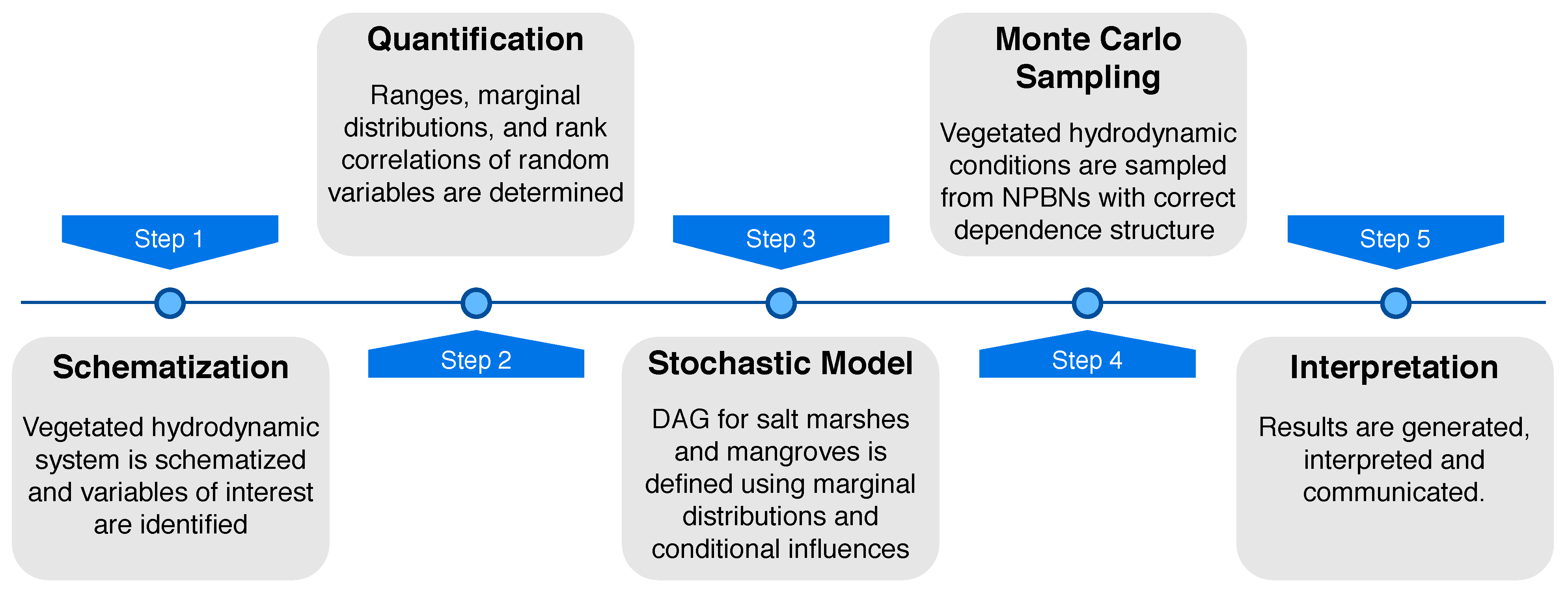
Vegetated hydrodynamic systems were schematized, parameterized, and probabilistically modeled in the user-defined random variable mode of UNINET [57,59], see overall methodology in Figure 2. The parameterization was conducted for benthic, submerged, and emergent vegetation, and the system was categorized into three variable families: (i) hydrodynamic, (ii) vegetation, and (iii) hybrid (dike) variables. Each variable was described with a continuous marginal distribution along with (conditional) rank correlations among variables determined from literature, data, or “in-house” expert judgment. Gaussian-copula based nonparametric Bayesian networks were created for submerged (salt marshes) and emergent (mangroves) vegetation, both combined with a seagrass meadow in the lower intertidal. Monte Carlo sampling was carried out from the NPBNs which resulted in realistic physical conditions sampled from a stochastic model that takes multivariate dependence into account.

2.1. System Schematization and Parameterization

To simplify the system hydrophysically, a 1-dimensional cross-shore profile and a dike without a berm were schematized. Vegetation was schematized as rigid cylinders and seagrasses, saltmarshes, and mangroves were modeled as benthic, submerged, and emergent vegetation respectively.

2.1.1. Schematization

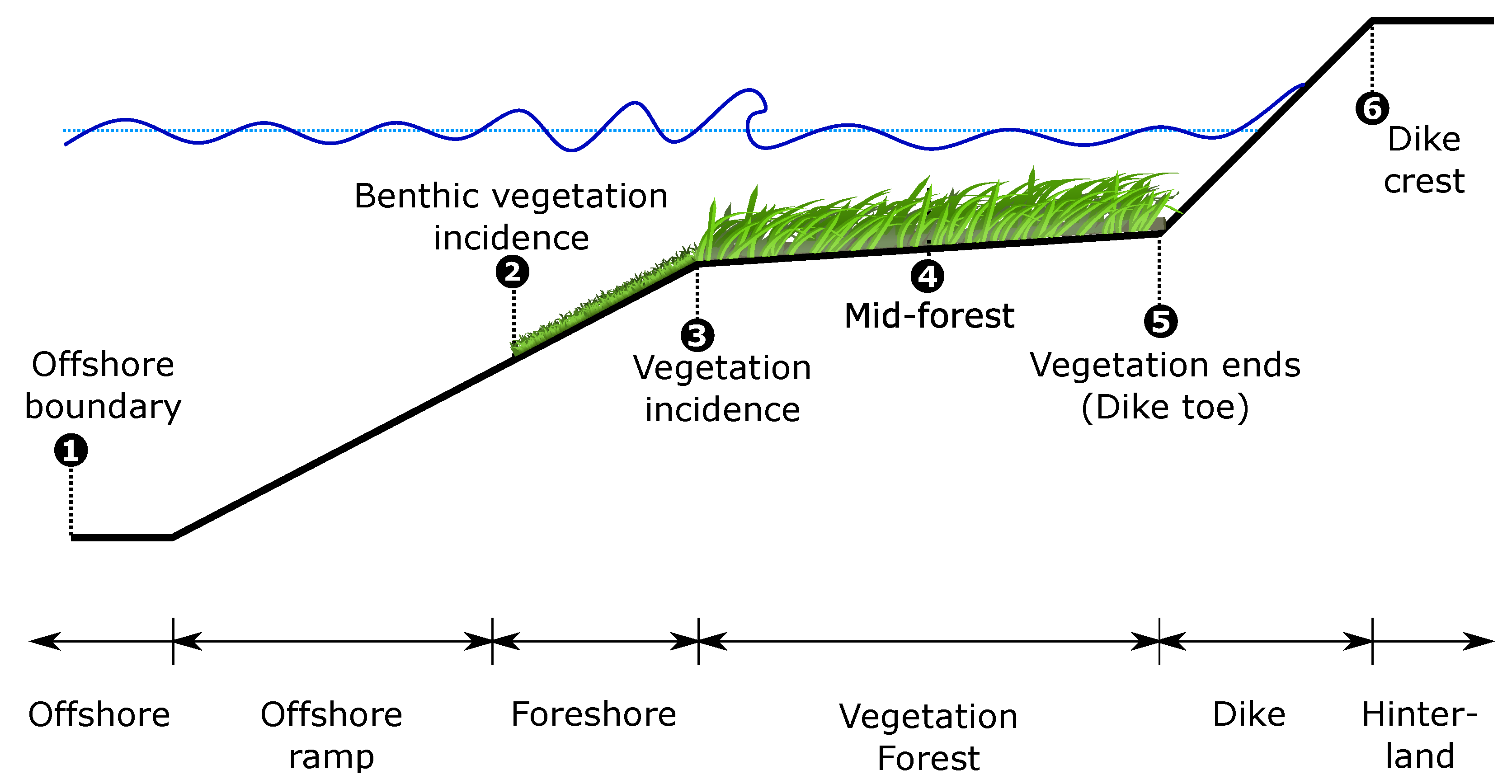
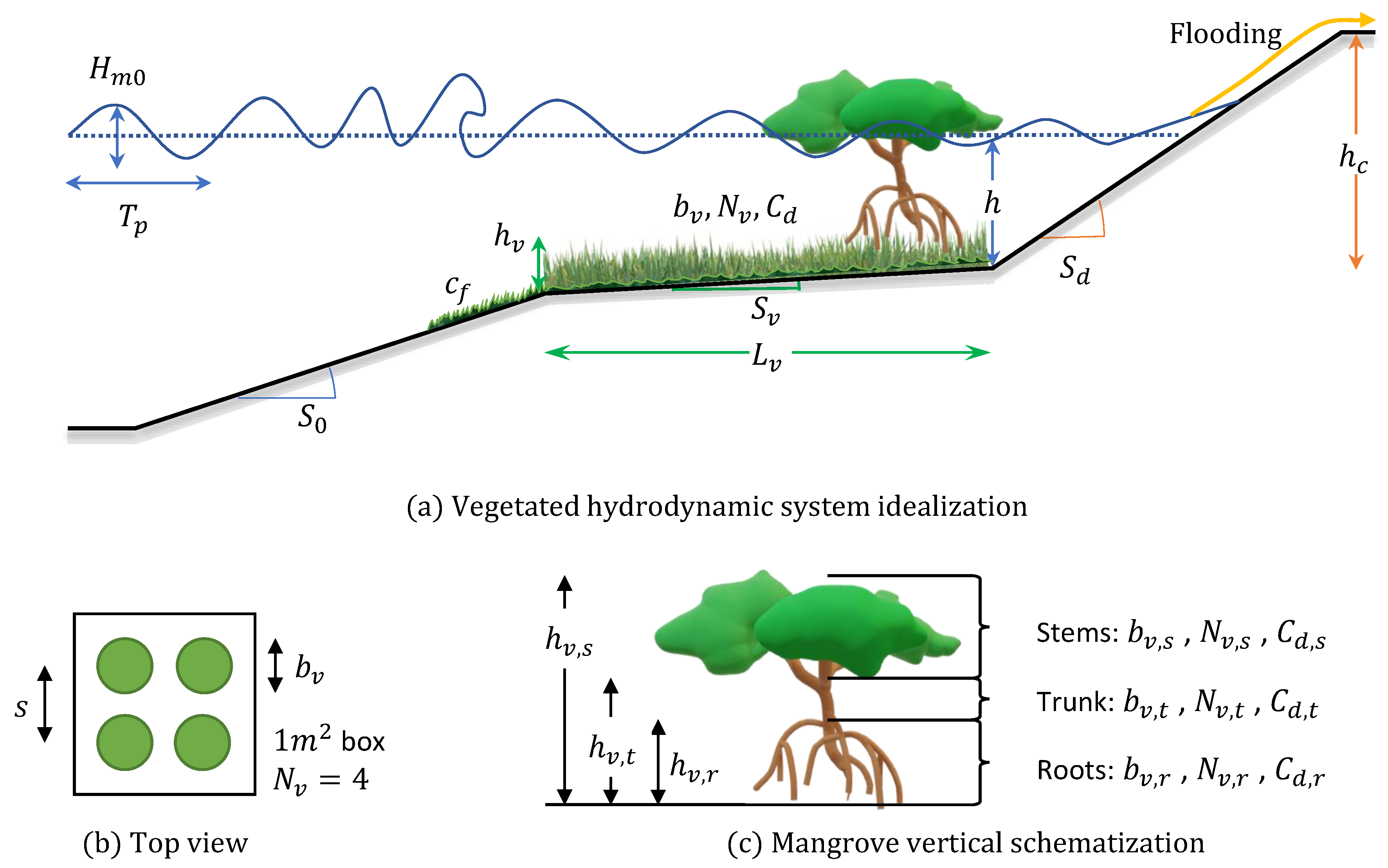
The schematization in Figure 3 was idealized and divided into 6 segments based on the dominant physical and hydrodynamic processes. Hydrodynamic boundary conditions were defined at the offshore boundary. After nearshore transformation on the ramp, waves reached till the point where they started to “feel” the bottom. At this point on the foreshore, bottom friction started playing a role, mimicking both bed roughness and the benthic vegetation. Waves then encountered a hybrid flood defense system, consisting of mature vegetation (a saltmarsh or mangrove forest) and a dike at the landward extent of vegetation, see Figure 3. The toe of the dike was fixed at $z_{toe}=0$ m and the rest of the depths were calculated as positive upwards from this reference.

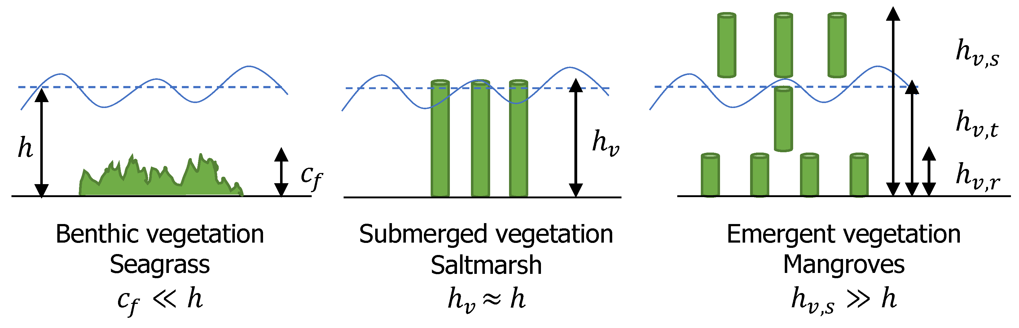
Vegetation was schematized based on the relative depth between water and vegetation height. Seagrasses were idealized as benthic vegetation, salt marshes as fully submerged with the water depth approaching vegetation height, and mangroves as emergent vegetation with multiple vertical layers, see Figure 4. Seagrasses were modeled as bed friction, salt marshes and mangroves as rigid cylinders parameterized by stem height, drag coefficient, frontal width, and vegetation density.

2.1.2. Variable Families

The minimum required number of primary variables which could sufficiently describe the hydrodynamic forcing, a vegetation field, and a dike were used (Figure 5). Variations of these variables could reproduce a variety of biohydrophysical conditions observed across the globe. All variables used are listed hereunder:

• Hydrodynamic: Offshore wave height $\left(H_{m0}\right)$, peak wave period $\left(T_p\right)$, water depth $\left(h\right)$, and offshore slope $\left(S_0\right)$ were grouped as hydrodynamic variables.
• Vegetation: Vegetation forest length $\left(L_v\right)$ and vegetation slope $\left(S_v\right)$ were general vegetation variables which represented forest characteristics for both saltmarshes and mangroves.

  -

  Benthic vegetation was represented through dimensionless bed friction coefficient $\left(c_f\right)$.

  -

  Submerged vegetation was parameterized by vegetation height $\left(h_v\right)$, frontal width $\left(b_v\right)$, vegetation density $\left(N_v\right)$, and drag coefficient $\left(C_d\right)$.

  -

  Emergent vegetation had three sub categories for each of the vertical layers.

  *

  Stem height $\left(h_{v,s}\right)$, stem frontal width $\left(b_{v,s}\right)$, stem density $\left(N_{v,s}\right)$, and stem drag coefficient $\left(C_{d,s}\right)$ were put in place for the top layer of mangroves.

  *

  Trunk height $\left(h_{v,t}\right)$, trunk frontal width $\left(b_{v,t}\right)$, trunk density $\left(N_{v,t}\right)$, and trunk drag coefficient $\left(C_{d,t}\right)$ were introduced to schematize the trunk.

  *

  Mangrove roots had height $\left(h_{v,r}\right)$, frontal width $\left(b_{v,r}\right)$, density $\left(N_{v,r}\right)$, and drag coefficient $\left(C_{d,r}\right)$.

• Hybrid: Lastly, dike slope $\left(S_d\right)$ and crest level $\left(h_c\right)$ were labeled as hybrid variables.

Hydrodynamic Variables

Generally, wave heights are Rayleigh distributed for a random sea-state but they are Weibull distributed for long time scales [21,66]. Hence, global trends and distribution of wave height and corresponding peak wave periods [67,68] were adopted for $H_{m0}$ and $T_p$. Water depth accounts for the mean sea level, storm surges, tidal fluctuations, and sea level rise due to climate change. Water depth was kept uniformly distributed within a range that was obtained using a breaker index-based $({\gamma }_b=H_{rms}/h=0.8)$ back calculation so that the waves break near the toe of the dike.

Vegetation Variables

The values for the vegetation variables were synthesized from more than 25 studies to parameterize the vegetation, see Table 1. In addition, similar synthesis results from [31] for salt marshes and from [69] for mangroves were augmented into a literature meta-analysis and were used as a basis to parameterize most of the vegetation variables. However, individual studies that specifically covered global distribution of a certain parameter were preferred over the meta-analysis of this study, e.g., see [27] for mangrove canopy heights. Moreover, some data was modified during the synthesizing process to optimally fit the study scope. For example, large forest lengths (up to 30 km) [40,65], were curtailed to 1.5 km assuming that the vulnerability of communities protected by such large vegetation forest is negligible. Or dimensionless friction coefficient was calculated using $c_f=\frac{g{n}^2}{h^{1/3}}$ from the range of Manning’s coefficients $\left(n\right)$ produced by [70,71] for various vegetation.

Hybrid Variables

Dike crest levels were defined as the maximum vertical distances relative to the dike toe and were critical for determining the run-up extent. The maximum crest level was estimated by adding maximum water depth, maximum wave height, and minimum free-board. The dike slope was used to determine the horizontal distance between the toe of the dike and the crest. Typical ranges of dike slopes and minimum free-board were determined by asking design experts who practice dike design in accordance with criteria mentioned by [72].

2.2. Stochastic Model Setup

The stochastic model was made in the user-defined mode of UNINET in order to sample varied vegetated-hydrodynamic conditions. UNINET models nonparametric Bayesian networks which are from the family of hybrid BNs characterized by Gaussian copulas. Setting-up the directed acylcic graph of a NPBN requires marginal distributions of random variables as nodes and (conditional) rank correlations as influences on arcs. Continuous marginal distributions of the random variables (nodes) were defined from a range of parametric distributions available in UNINET, see

Table 2. Ranges and marginal distributions for variables in the vegetated hydrodynamic system. Refer to Table A1 for complete description of variable distributions.

Variable	Symbol	Unit	Range	Distribution	Source
Offshore Wave Height	$H_{m0}$	m	$0.1$ to $\approx 8$	Weibull	[21]
Peak wave period	$T_p$	s	1 to $\approx 30$	Gamma	[22]
Water depth	h	m	$0.01$ to 5	Uniform	[23]
Offshore slope	$S_0$	–	$\frac{1}{10}$ to $\frac{1}{500}$	Beta	Experts
Vegetation forest length	$L_v$	m	1 to 1500	Beta	[65]
Vegetation slope	$S_v$	–	$\frac{1}{500}$ to $\frac{1}{1000}$	Beta	Expert
Benthic Seagrasses
Friction coefficient	$c_f$	–	$0.01$ to $0.1$	Beta	[70]
Submerged Saltmarshes
Vegetation height	$h_v$	m	$0.02$ to $1.75$	Beta	[31]
Frontal width	$b_v$	m	$0.0001$ to $0.025$	Beta	[31]
Vegetation density	$N_v$	stems/m${}^2$	10 to 2000	Beta	[31]
Drag coefficient	$C_d$	–	$0.1$ to 3	Beta	[26]
Emergent Mangroves
Stems height	$h_{v,s}$	m	$0.1$ to 5	Beta	[27]
Stems frontal width	$b_{v,s}$	m	$0.01$ to $0.25$	Beta	[69]
Stems density	$N_{v,s}$	stems/m${}^2$	$0.1$ to 100	Beta	[69]
Stem drag coefficient	$C_{d,s}$	–	$0.1$ to $2.5$	Beta	[26]
Trunk height	$h_{v,t}$	m	$0.1$ to 4	Beta	[27]
Trunk frontal width	$b_{v,t}$	m	$0.1$ to $0.8$	Beta	[73]
Trunk density	$N_{v,t}$	trunk/m${}^2$	$0.5$ to 5	Beta	[69]
Trunk drag coefficient	$C_{d,t}$	–	$0.1$ to 3	Beta	[26]
Roots height	$h_{v,r}$	m	$0.2$ to 6	Beta	[27]
Roots frontal width	$b_{v,r}$	m	$0.004$ to $0.1$	Beta	[69]
Roots density	$N_{v,r}$	roots/m${}^2$	1 to 250	Beta	[69]
Roots drag coefficient	$C_{d,r}$	–	$0.1$ to 4	Beta	[26]
Hybrid
Dike slope	$S_d$	–	$\frac{1}{2}$ to $\frac{1}{10}$	Beta	Experts
Crest level	$h_c$	m	1 to 20	Gaussian	Expert

. For influences (arcs), bivariate rank correlations were determined through data or expert judgment. Once the DAG was setup, analytical conditioning of the NPBN was performed by UNINET and Monte Carlo samples of variables were generated which established the varied vegetated hydrodynamic conditions.

2.2.1. Marginal Distributions

While determining the marginal distributions, as presented in Table 2, preference was given to published studies that explicitly provide parameterized distributions for variables, e.g., offshore wave height [21], peak wave period [22], and mangrove trunk height [27]. Secondly, when explicit estimates of distributions were not available, data over multiple spatial domains and long temporal scales was used. Only hydrodynamic data of such sort was available which was used to cross-check the marginal distribution and was instrumental in determining rank correlations. However, when multispatiotemporal data was not available, local datasets at specific locations were used to derive the first best assessment of the distributions, e.g., salt marsh height, frontal width, and density. If no data was available, literature was consulted to carry out a meta-analysis aimed to identify general trends about variability of a variable which could be used to infer distributions, e.g., drag coefficient, vegetation, and offshore slope. Except for the variables from published studies, beta distribution was preferred for most of other variables due to its ability to give control of both the bounds (range) and the variability within the bounds (density function).

2.2.2. Correlations and Copulas

Bivariate rank correlations were calculated from various sources of data and in-house expert judgment as presented in Table 2 and elaborated in following sections. Moreover, in case of conditional dependence, where a child node is dependent on more than one parent node, recursive formula [56,64] in Equation (1) was used to calculate conditional rank correlations. For instance, conditional rank correlation for frontal width and vegetation density given vegetation height $(b_v,N_v|h_v)$ was calculated using bivariate rank correlations of $(h_v,b_v)$, $(h_v,N_v)$, and $(N_v,h_v)$.

$${\rho }_{12|3}=\frac{{\rho }_{12}-{\rho }_{13}·{\rho }_{23}}{\sqrt{\left(1-{\rho }_{13}^2\right)·\left(1-{\rho }_{23}^2\right)}}$$

(1)

where ${\rho }_{12|3}$ is the conditional rank correlation coefficient of random variables $X_1$ and $X_2$ given $X_3$.

Data Processing

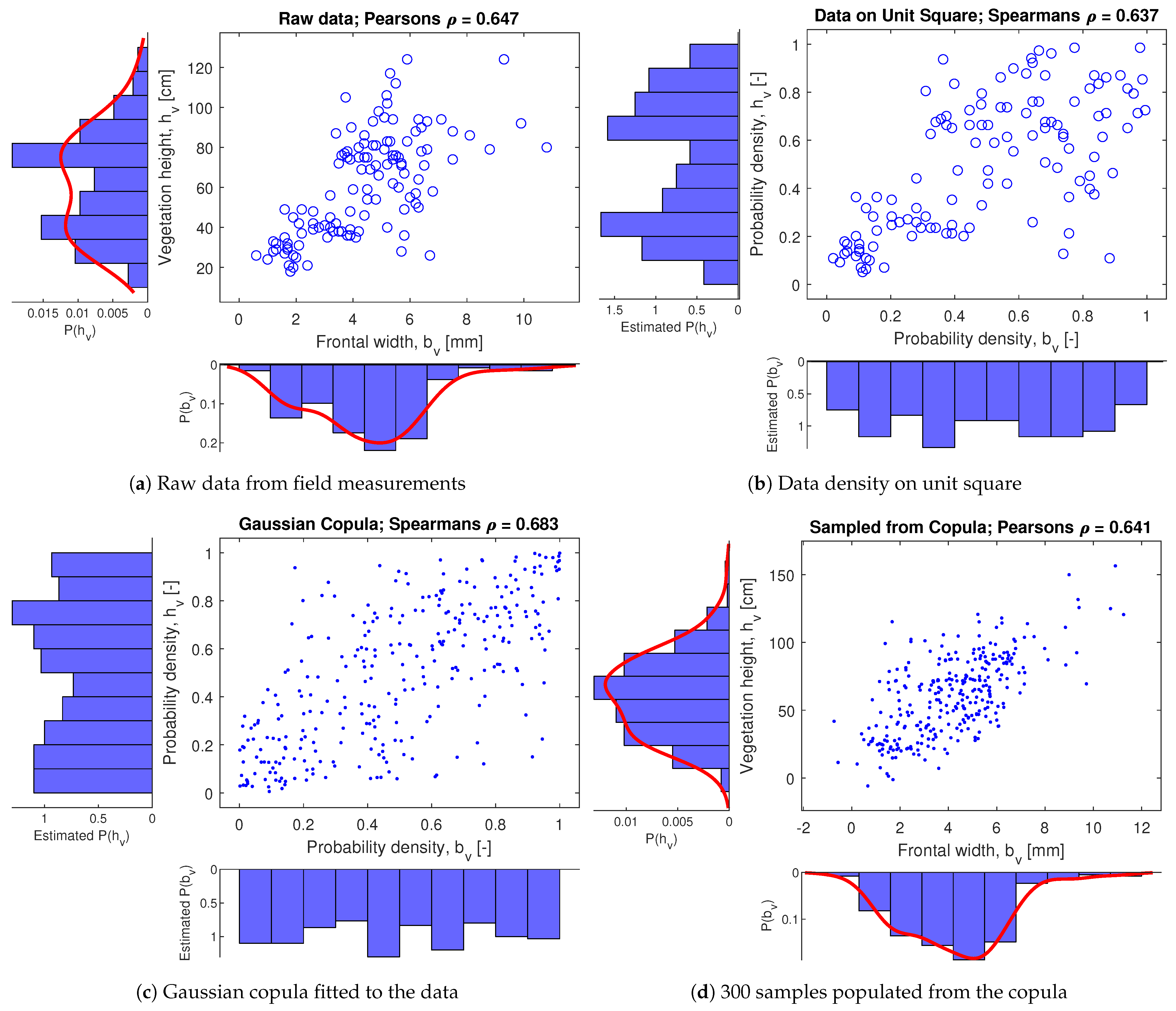
Raw field data was processed to acquire correlation coefficients and synthetic data sampled from an estimated Gaussian copula. An example of data processing is presented for two vegetation variables: vegetation height $\left(h_v\right)$ and frontal width $\left(b_v\right)$, see Figure 6. The field vegetation data for Chesapeake Bay in the north-eastern part of the US was used from four different stations along a transect containing Spartina alterniflora and Spartina patens species. The raw data in Figure 6a was transformed to the unit square based on its cumulative distribution function (Figure 6b) and the Gaussian copula was estimated (Figure 6c). This copula together with the marginal distributions may be used to sample synthetic data. In Figure 6d, random sampling for both variables was transformed back to original units through the inverse of the cumulative distributions function. Similar analysis of both $h_v$ and $b_v$ was done in relation to vegetation density and, overall, the rank correlations obtained from this data source were of $(h_v,b_v)$, $(h_v,N_v)$, and $(N_v,h_v)$.

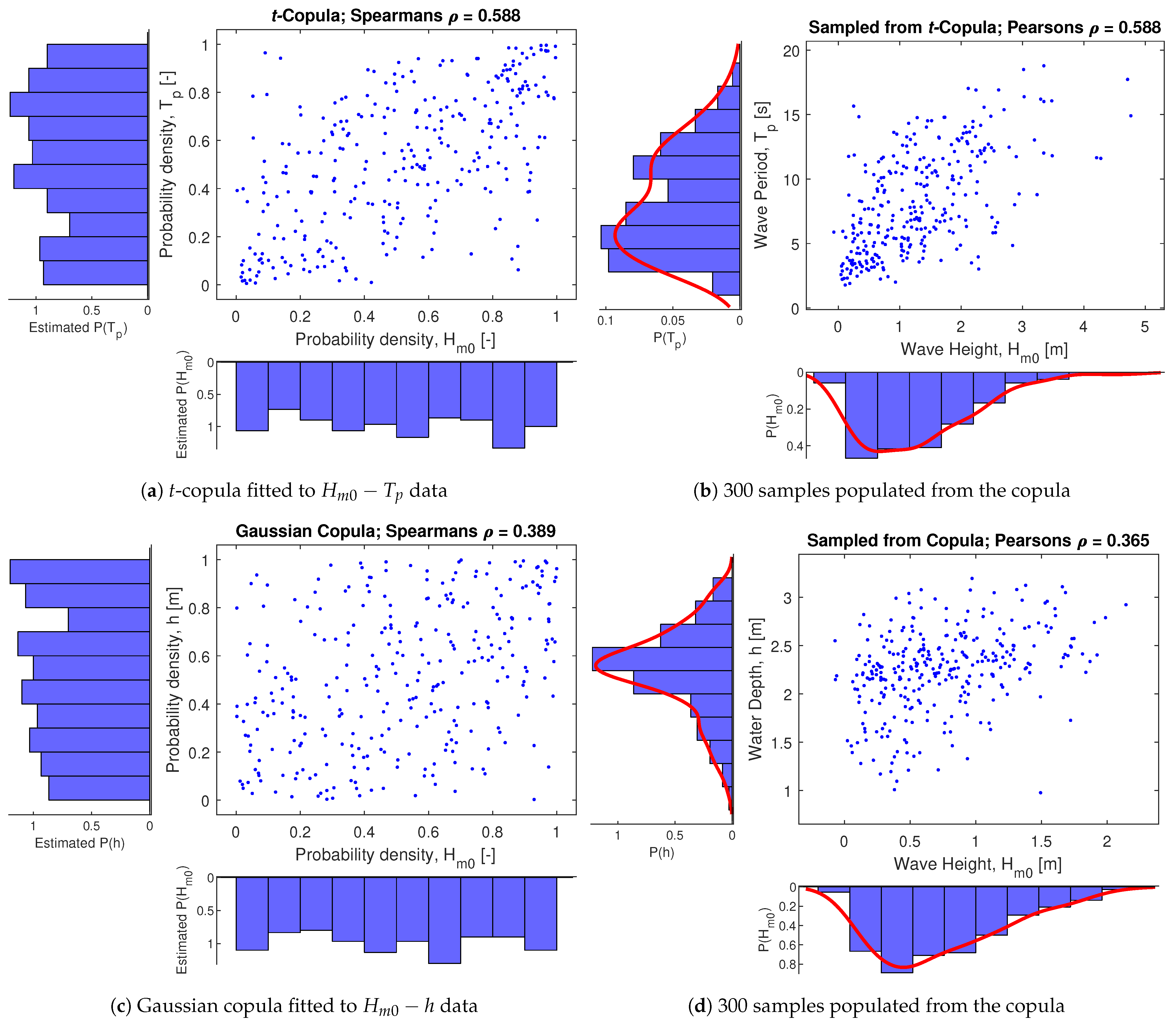
For the hydrodynamic variables, time-series data was obtained for 10 distinct locations over 25 years with 3-hour resolution from waveclimate.com and treated in a similar manner as explained for the vegetation variables. The 10 major deltas with vegetation on foreshores were selected from [74] and representative average values for wave conditions are presented in

Table 3. World wave climate based on ten cities in biggest deltas having vegetated foreshores.

City, Country	Location	Vegetation	Wave Height $\left({\mathit{H}}_{\mathit{m}0}\right)$ [m]		Wave Period $\left({\mathit{T}}_{\mathit{p}}\right)$ [s]
			Mean	Variance	Mean	Variance
Los Angeles, USA	33° N 120° W	Saltmarsh	2.17	0.73	11.99	9.73
Mérida, Mexico	21° N 090° W	Seagrass	0.44	0.07	4.13	2.55
São Luís, Brazil	01° S 043° W	Mangroves	1.63	0.15	8.71	6.77
Texel, Netherlands	53° N 005° E	Saltmarsh	0.82	0.46	5.91	5.03
Lagos, Nigeria	05° N 003° E	Seagrass	1.34	0.13	12.69	4.30
Dubai, UAE	25° N 054° E	Seagrass	0.60	0.18	4.99	1.14
Karachi, Pakistan	24° N 067° E	Mangroves	1.35	1.38	10.39	11.50
Shanghai, China	32° N 122° E	Saltmarsh	0.95	0.32	5.45	3.40
Surabaya, Indonesia	06° S 113° E	Mangroves	0.63	0.17	4.32	1.44
Sydney, Australia	34° S 152° E	Saltmarsh	2.15	0.87	9.29	8.99

. The rank correlation obtained from this data source, as presented in Figure 7, were $\rho (H_{m0},T_p)$, $\rho (H_{m0},h)$, and $\rho (T_p,h)$.

Expert Judgment

In case of unavailability of data or literature, the classical model of expert judgment is an option [55,75,76,77,78,79] to determine rank correlations between two or more variables. In this case, the classical model could not be fully implemented due to limited resource. However, in-house expert judgment was incorporated through verbal communication with experts and elicitation from a combination of general trends from literature. For example, a higher water level would require a higher dike crest level hence the rank correlation for $(h,h_c)$ was defined positive. Overall, individual estimates of experts about the nature (positive or negative) and strength (value) of correlations were collated together to derive estimates of dependence among variables. The correlations defined based on expert judgment, as mentioned in Table 4, were mainly for vegetation and hybrid variables.

The resulting ranges, distributions, and correlations from literature meta-analysis, data processing, and expert judgment are presented in Table 2 and Table 4 along with their main source. These quantification results formed the basis for setting up the nonparametric Bayesian networks for salt marshes and mangroves as presented in Figure 8 and Figure 9 respectively.

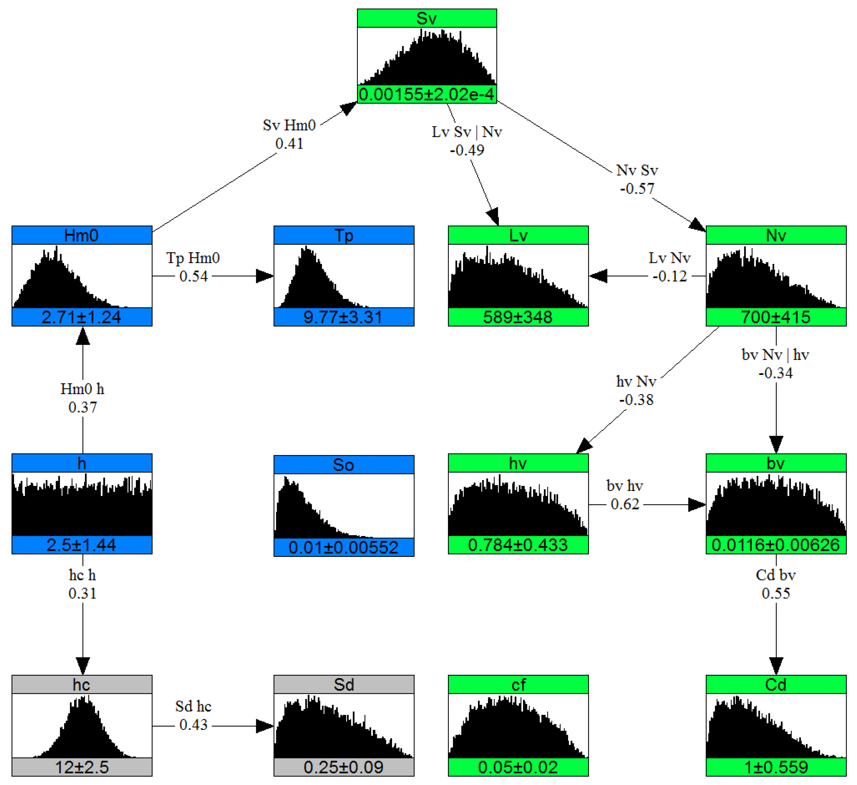
Figure 8. Nonparametric Bayesian network for salt marsh environment [1,30]. The boxes represent nodes (variables with their marginal distributions) and lines represent influences (rank correlations). Color indicates different components in the system: blue for hydrodynamics, gray for dike, light green for seagrass-saltmarsh variables.

Figure 8. Nonparametric Bayesian network for salt marsh environment [1,30]. The boxes represent nodes (variables with their marginal distributions) and lines represent influences (rank correlations). Color indicates different components in the system: blue for hydrodynamics, gray for dike, light green for seagrass-saltmarsh variables.

Figure 9. Nonparametric Bayesian network for mangroves environment. The boxes represent nodes (variables with their marginal distributions) and lines represent influences (correlations). Color indicates different components in the system: blue for hydrodynamics, gray for dike, light green for general vegetation variables, dark green for stems, brown for trunk, and yellow for roots of mangroves.

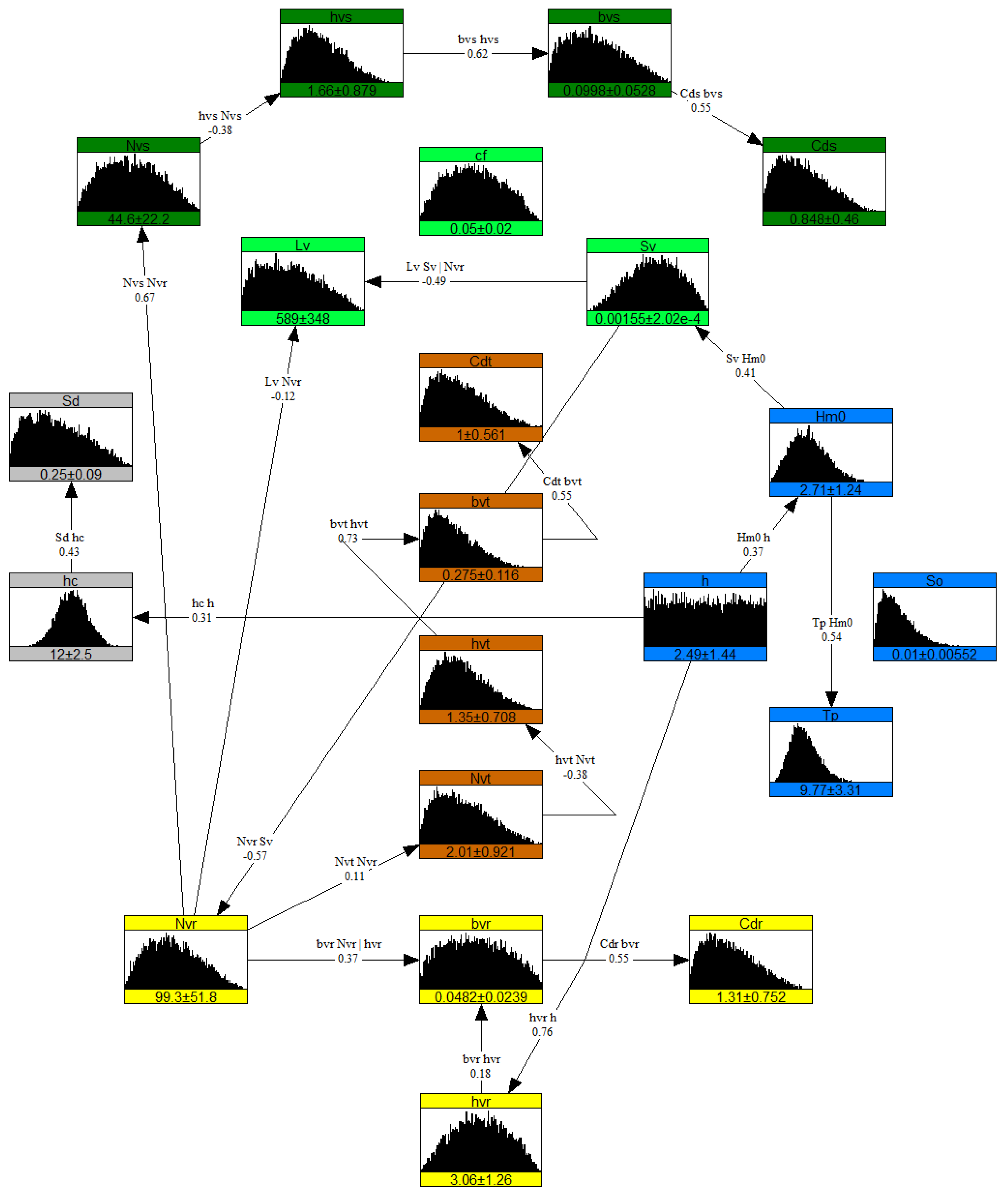
Figure 9. Nonparametric Bayesian network for mangroves environment. The boxes represent nodes (variables with their marginal distributions) and lines represent influences (correlations). Color indicates different components in the system: blue for hydrodynamics, gray for dike, light green for general vegetation variables, dark green for stems, brown for trunk, and yellow for roots of mangroves.

Table 4. Rank correlations among variables in salt marsh system. See Figure 9 for correlations of mangrove system variables.

Correlations	Nature	Coefficient	Source
$H_{m0}\leftrightarrow T_p$	+	0.54	Data
$H_{m0}\leftrightarrow h$	+	0.37	Data
$S_v\leftrightarrow H_{m0}$	+	0.41	Expert Judgment
$S_v\leftrightarrow L_v$	−	0.33	Expert Judgment
$S_v\leftrightarrow N_v$	−	0.57	Expert Judgment
$h_v\leftrightarrow b_v$	+	0.62	Data
$N_v\leftrightarrow h_v$	−	0.38	Data
$N_v\leftrightarrow b_v$	−	0.48	Data
$N_v\leftrightarrow L_v$	−	0.12	Expert Judgment
$b_v\leftrightarrow C_d$	+	0.55	Expert Judgment
$h\leftrightarrow h_c$	+	0.31	Expert Judgment
$S_d\leftrightarrow h_c$	+	0.43	Expert Judgment

Table 4. Rank correlations among variables in salt marsh system. See Figure 9 for correlations of mangrove system variables.

Correlations	Nature	Coefficient	Source
$H_{m0}\leftrightarrow T_p$	+	0.54	Data
$H_{m0}\leftrightarrow h$	+	0.37	Data
$S_v\leftrightarrow H_{m0}$	+	0.41	Expert Judgment
$S_v\leftrightarrow L_v$	−	0.33	Expert Judgment
$S_v\leftrightarrow N_v$	−	0.57	Expert Judgment
$h_v\leftrightarrow b_v$	+	0.62	Data
$N_v\leftrightarrow h_v$	−	0.38	Data
$N_v\leftrightarrow b_v$	−	0.48	Data
$N_v\leftrightarrow L_v$	−	0.12	Expert Judgment
$b_v\leftrightarrow C_d$	+	0.55	Expert Judgment
$h\leftrightarrow h_c$	+	0.31	Expert Judgment
$S_d\leftrightarrow h_c$	+	0.43	Expert Judgment

3. Results

This work aimed to obtain a better understanding of mangroves and salt marshes and parameters influencing wave attenuation by these ecosystems. This was approached through constructing a stochastic model for salt marshes and mangroves in the form of nonparametric Bayesian networks which capture the dependence among variables of interest. The NPBNs could be used to sample varied vegetated hydrodynamic conditions that tend to coexist in physically realistic windows.

3.1. Vegetated Hydrodynamic System

The nonparametric Bayesian network representing salt marsh environment is presented in Figure 8. Overall, the NPBN quantifies the influences between the vegetation and the hydrodynamic variables which eventually captures the underlying dependence of the system. Interactions among groups of variables (vegetation and hybrid) are linked through hydrodynamic variables as the incoming energy determines both dike crest levels and foreshore slopes. Stem width shows conditional dependence on other variables as it has two parent nodes, i.e., stem height and vegetation density. Variables near the offshore boundary, such as offshore slope and seagrass bed roughness, do not interact actively with the rest of the system and therefore operate as independent variables.

Similarly, for mangrove environments the NPBN is presented in Figure 9. The mangrove variables were divided into three layers (roots, trunk, and stem) due to the differences in their phytomorphological characteristics. Root density plays an important role in this NPBN as it links vegetation slope and forest length to the root layer and further links all mangrove layers to each other. This allows for the maintenance of the harmony between individual plant characteristics and the overall forest characteristics in sampled conditions. Similarly, using the relative emergent property of mangroves, the root height is linked to water depth that conceptually connects hydrodynamic variables to vegetation variables.

Accounting for the multivariate-dependence enables the generation of Monte Carlo samples of variables, which constitute varied boundary conditions. This, for instance, in the case of relatively more energetic hydrodynamic conditions generates samples of reflective beaches, higher and steeper dikes, and higher mangrove roots. Similarly, root variables influence trunk and stem variables as root structure categorizes mangroves into juvenile or mature mangrove types.

3.2. Dependence

The NPBNs are based on a consistent joint probability distribution of all the variables in the network correlated to one another. Due to conditional dependence, more correlations were revealed apart from the ones that were already defined to setup the model, e.g., stem height and drag coefficient. This resulted in a symmetric correlation matrix which indicates the dependence among all variables, see

Table 5. Correlation matrix of stochastic model for salt marshes, also see Figure 10. Highest correlation is 1.00, lowest is 0.00. Positive and negative values show positive and negative correlations. The correlations other than the ones in Figure 8 have been calculated using Equation (1). Similar correlation matrix for mangroves nonparametric Bayesian network (NPBN) is presented in Supplementary Materials.

	${\mathit{H}}_{\mathit{m}0}$	h	${\mathit{T}}_{\mathit{p}}$	${\mathit{c}}_{\mathit{f}}$	${\mathit{S}}_{\mathit{d}}$	${\mathit{h}}_{\mathit{c}}$	${\mathit{L}}_{\mathit{v}}$	${\mathit{N}}_{\mathit{v}}$	${\mathit{C}}_{\mathit{d}}$	${\mathit{h}}_{\mathit{v}}$	${\mathit{b}}_{\mathit{v}}$	${\mathit{S}}_{\mathit{v}}$	${\mathit{S}}_0$
$H_{m0}$	1.00	0.37	0.54	0.00	0.05	0.12	−0.14	−0.24	0.07	0.09	0.12	0.41	0.00
h	0.37	1.00	0.20	0.00	0.14	0.31	−0.05	−0.09	0.03	0.04	0.05	0.16	0.00
$T_p$	0.54	0.20	1.00	0.00	0.03	0.07	−0.08	−0.13	0.04	0.05	0.07	0.23	0.00
$c_f$	0.00	0.00	0.00	1.00	0.00	0.00	0.00	0.00	0.00	0.00	0.00	0.00	0.00
$S_d$	0.05	0.14	0.03	0.00	1.00	0.43	−0.01	−0.01	0.00	0.01	0.01	0.02	0.00
$h_c$	0.12	0.31	0.07	0.00	0.43	1.00	−0.02	−0.03	0.01	0.01	0.01	0.05	0.00
$L_v$	−0.14	−0.05	−0.08	0.00	−0.01	−0.02	1.00	−0.12	0.03	0.05	0.06	−0.32	0.00
$N_v$	−0.24	−0.09	−0.13	0.00	−0.01	−0.03	−0.12	1.00	−0.27	−0.38	−0.48	−0.57	0.00
$C_d$	0.07	0.03	0.04	0.00	0.00	0.01	0.03	−0.27	1.00	0.35	0.55	0.16	0.00
$h_v$	0.09	0.04	0.05	0.00	0.01	0.01	0.05	−0.38	0.35	1.00	0.62	0.22	0.00
$b_v$	0.12	0.05	0.07	0.00	0.01	0.01	0.06	−0.48	0.55	0.62	1.00	0.28	0.00
$S_v$	0.41	0.16	0.23	0.00	0.02	0.05	−0.32	−0.57	0.16	0.22	0.28	1.00	0.00
$S_0$	0.00	0.00	0.00	0.00	0.00	0.00	0.00	0.00	0.00	0.00	0.00	0.00	1.00

for the correlation matrix of the salt marsh system. A value close to 1.0 represents the strongest correlation, e.g., self-correlation on the diagonal, and a value close to 0.0 represents the weakest correlation, e.g., $c_f$ and $S_d$.

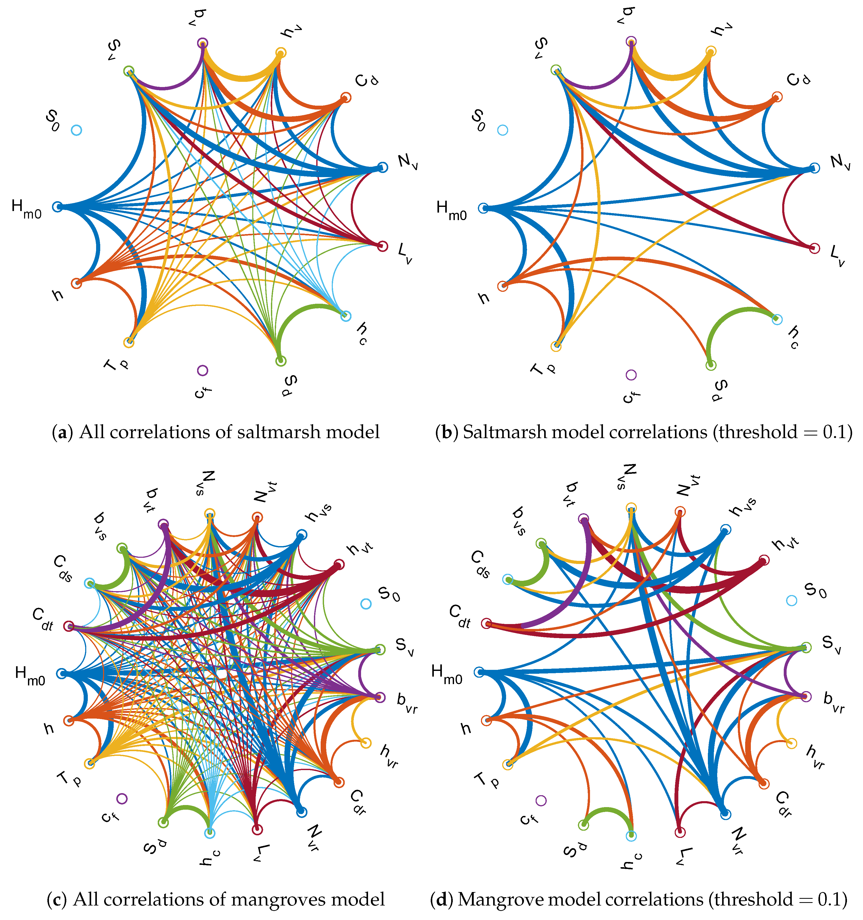
The correlation matrices generated by UNINET were transformed to adjacency matrices (which use absolute values of correlations) and have been plotted in Figure 10 for both the salt marsh and mangroves NPBNs. Figure 10a,c show all possible correlations among variables. The extensive amount of influences show the inherent complexity of the vegetated hydrodynamic system which is undermined when it is studied using deterministic methods. Dominant correlations were filtered out by fixing the correlation threshold to 0.1, see Figure 10b for salt marshes and Figure 10d for mangroves.

The strength of copulas and dependence modeling allows us to demonstrate the influences which are not initially perceived. For salt marshes an example could be the correlations of wave height with drag coefficient, vegetation height, frontal width, dike slope, and crest level. The strongest conditional dependence is between drag coefficient and vegetation height, followed by wave height and vegetation density, drag coefficient and vegetation density, and vegetation slope and frontal width in salt marshes. For mangroves, the strongest of such “non parent-child” correlations is between trunk height and trunk drag coefficient while other examples include wave height and root height, stem density and vegetation slope, and trunk frontal width and trunk density. This means that the effects on the system of all such correlated variables shown in Figure 10b,d should not be studied in isolation from the other variables, otherwise the true system response (e.g., wave damping) would not be revealed.

3.3. Realistic Boundary Conditions

Analytical conditioning of the stochastic model and Monte Carlo sampling (a process of picking up random values from a probabilistically interpreted system) resulted in logical combinations of variables. Due to the correlations and the joint distribution, two variables are “tied-up” together such that the range of a variable only coexists within a certain range of another variable, e.g., high waves with long periods.

Table 6. Monte Carlo samples from NPBN for salt marsh environments.

Run	${\mathit{H}}_{\mathit{m}0}$	${\mathit{T}}_{\mathit{p}}$	h	${\mathit{S}}_0$	${\mathit{h}}_{\mathit{v}}$	${\mathit{b}}_{\mathit{v}}$	${\mathit{N}}_{\mathit{v}}$	${\mathit{S}}_{\mathit{v}}$	${\mathit{L}}_{\mathit{v}}$	${\mathit{C}}_{\mathit{d}}$	${\mathit{c}}_{\mathit{f}}$	${\mathit{S}}_{\mathit{d}}$	${\mathit{h}}_{\mathit{c}}$
1	2.32	11.5	0.39	0.024	0.259	0.006	417	0.00156	309.1	1.63	0.03	0.27	11.18
2	6.63	20.0	3.58	0.011	0.404	0.007	759	0.00165	342.7	1.52	0.072	0.29	13.05
3	3.37	14.2	4.86	0.006	0.911	0.012	1217	0.00131	1075.2	0.91	0.057	0.36	12.04
4	4.69	8.2	2.99	0.007	0.109	0.002	651	0.00175	478.2	0.72	0.061	0.3	14.8
5	0.15	5.1	0.53	0.007	0.667	0.013	1464	0.00118	168.3	1.73	0.079	0.12	12.69
6	1.29	8.5	0.81	0.021	0.653	0.021	372	0.00179	1310.3	1.98	0.052	0.15	11.63
7	1.95	8.9	0.84	0.021	0.147	0.010	125	0.00174	1224.4	1.37	0.093	0.16	13.17
8	7.14	13.0	2.23	0.005	1.625	0.024	504	0.00199	4.4	1.56	0.074	0.29	11.42
9	1.37	5.6	0.78	0.014	0.219	0.001	1311	0.00164	676.5	0.35	0.062	0.16	10.31
10	1.72	8.3	0.56	0.011	0.462	0.017	1086	0.00174	123.91	1.52	0.065	0.25	9.79
⋮	⋮	⋮	⋮	⋮	⋮	⋮	⋮	⋮	⋮	⋮	⋮	⋮	⋮
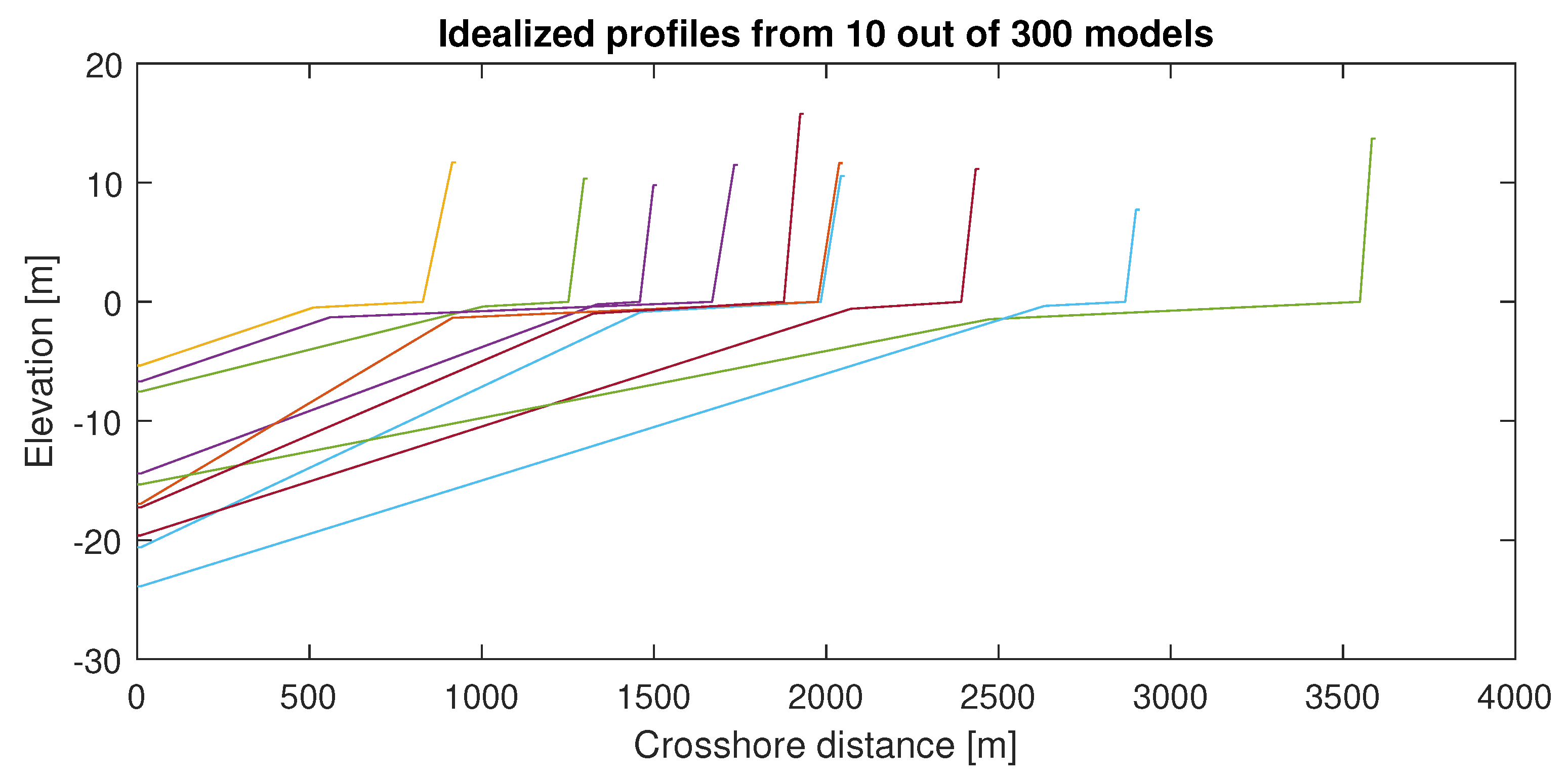
300	1.30	8.2	0.84	0.012	0.731	0.008	140	0.00164	1200.97	0.71	0.08	0.26	9.92

shows part of 300 physically realistic combinations of variables in saltmarsh environments representing boundary conditions which could potentially be used for hydrovegetation modeling. The sampled conditions represent combinations of hydrodynamic forcing, physical conditions, sea states, vegetation types, vegetation characteristics, and flood defense extents to cover the entire space of variations that would yield generalized results when analyzed further. An example of the sampling result could be seen in Figure 11 which shows combinations of foreshore slope, forest length, crest level, and dike slope.

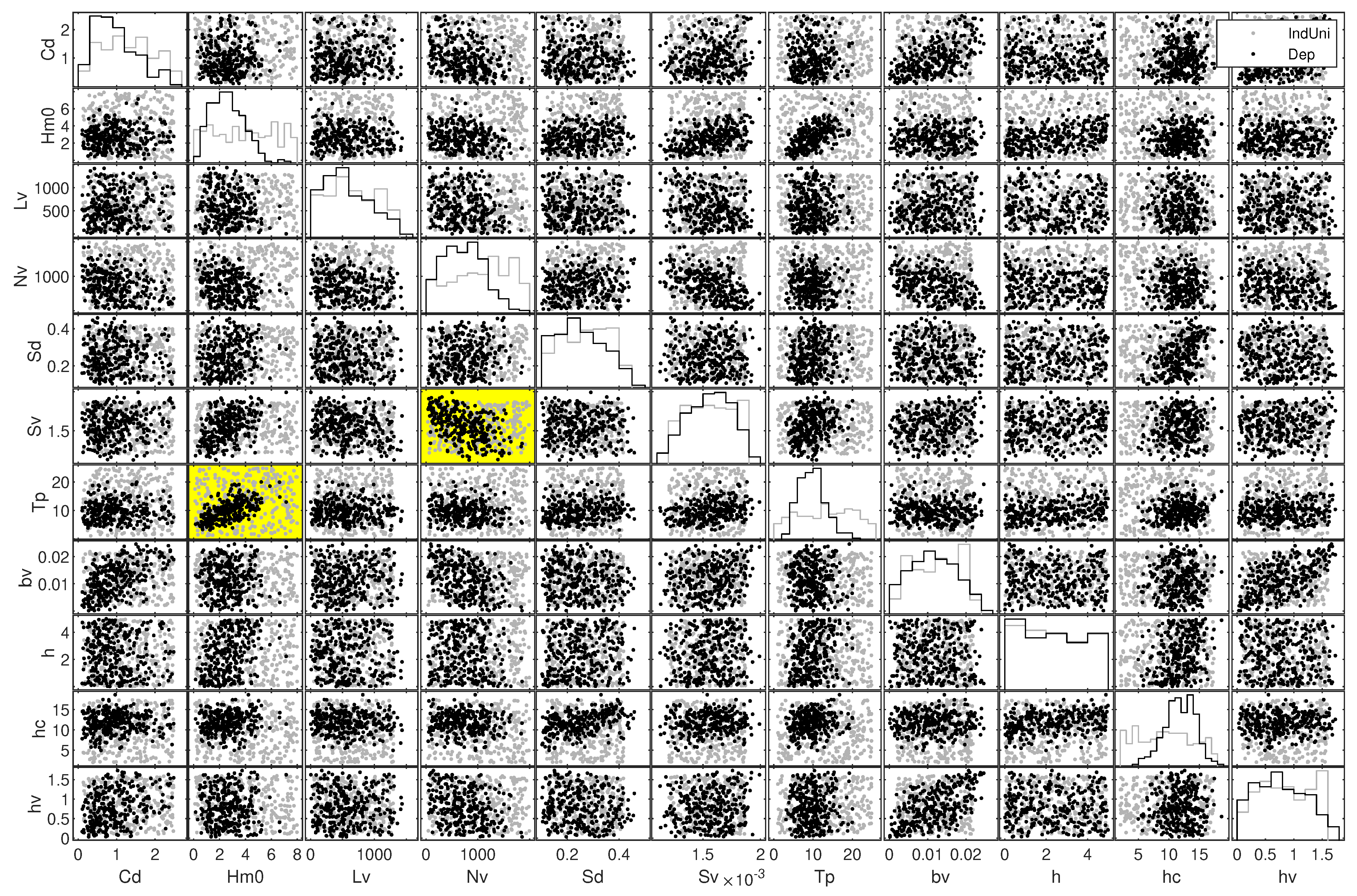
A comparison of the conditions sampled from the salt marsh NPBN as the ‘dependent case’ with the conditions sampled from an independent DAG with uniformly distributed variables as the "independent case" is presented in Figure 12. For the independent case, sampled combinations cover almost the complete sampling space whereas for the dependent case a variable-specific pattern exists. For example, wave heights and wave periods are not sampled in any recognizable trend for the independent case but the conditions sampled from the stochastic model show positive dependence such that there are almost no conditions sampled for high wave heights with low wave periods or vice versa. When compared to the data analyzed in this study and the published literature [23,80,81,82,83,84], the independent case deems to be unrealistic and the dependent case is in harmony for the variables whose dependence information is published. Hence, Figure 12 not only shows the pair-wise dependence of variables that emerged beyond the correlations initially defined, but also shows the realistic “windows” of variables where they coexist.

Moreover, the correlation for $\rho (H_{m0},T_p)$ was explicitly introduced while setting up the model but the results go beyond the specified correlations and reveal unspecified dependence. For instance, $\rho (H_{m0},N_v)$ was not specified initially but the corresponding plot in Figure 12 shows that for higher wave heights the vegetation density seems to have negative correlation and shows signs of tail dependence. This means that less vegetation is expected in high energetic environments. One possible explanation for this could be breakage or uprooting during storms as shown by [85].

4. Discussion

Vegetated hydrodynamic conditions sampled from the salt marsh and mangroves NPBNs could be further used for hydrovegetation numerical modeling, probabilistic modeling, or system-based sensitivity analysis. These conditions help to reduce the number of numerical simulations required to produce generalized results, aid probabilistic analysis in data-scarce environments, and provide a basis for a holistic system-based sensitivity analysis.

4.1. Value of Dependence Modeling Using Nonparametric Bayesian Networks

The value of dependence modeling of vegetated coastal systems for generating varied boundary conditions lies in obtaining physically realistic boundary conditions, which, when simulated, reduces bulk simulation time and increases the authenticity of overall system response. Using this approach will advance current modeling practice as conditions and values for sensitivity analysis are too often randomly or quickly selected instead of being informed by realistic situation. This asks for a good understanding of the biogeomorphological system and goes beyond standard modeling efforts by engineers solely. Hence, even in modeling studies inclusion of biophysical disciplines is essential to achieve realistic results that can be translated to situations encountered in real life.

4.1.1. Methodological Value

Many Bayesian network based studies for coastal applications have been published but nearly all of them use discrete Bayesian networks [47,48,49,50,51,52,53,54] except the very few recent ones which use NPBNs [86,87,88,89]. In discrete BNs, variables have to be discretized into bins where the number and sizes of the bins need to be correctly fine-tuned to ensure that each bin represents homogeneous information and has nearly similar impact on the child node. This introduces subjectivity as the decisions about bins could vary from person to person which adds another source of uncertainty in modeling discrete BNs. Belonging to the hybrid BNs family, NPBNs provide flexibility to incorporate both discrete and continuous marginal distributions in the same graph, thereby reducing the subjectivity and uncertainty.

4.1.2. Reduced Numerical Simulations

Using the sampled boundary conditions from the NPBNs can greatly reduce the number of simulations required to produce generalized results by orders of magnitude. The number of simulations $\left(N_s\right)$ required to quantify conditional probabilities of all variables in the system were in the order of ${\left(O\right)}^4$ to ${\left(O\right)}^5$ for [31,51,65]. The reason for such large $N_s$ is that it is a (sum-product) function of the number of variables and the number of permutations per variable, see Equation (2). If any of the two factors increase, the required number of simulations increases geometrically. With 13 variables of seagrass-saltmarshes system even if only 13 permutations per variable are numerically modeled, the number of simulations would go to a gigantic amount of $3.2·{10}^{14}$ which is computationally near to impossible. However, the number of simulations for the method presented in this study are only a function of the number of permutations due to the use of copulas. NPBNs can extract the dependence information even if all variables are varied at once; hence variables can be modeled as many times as the computational capacity permits.

$$N_s=\prod _{i=1}^n{v}_i$$

(2)

where, $N_s$ is total number of simulations, n is number of variables, i is a given variable, and v is the number of variations of a given variable [90].

4.1.3. Filling Information in Data-Scarce Environments

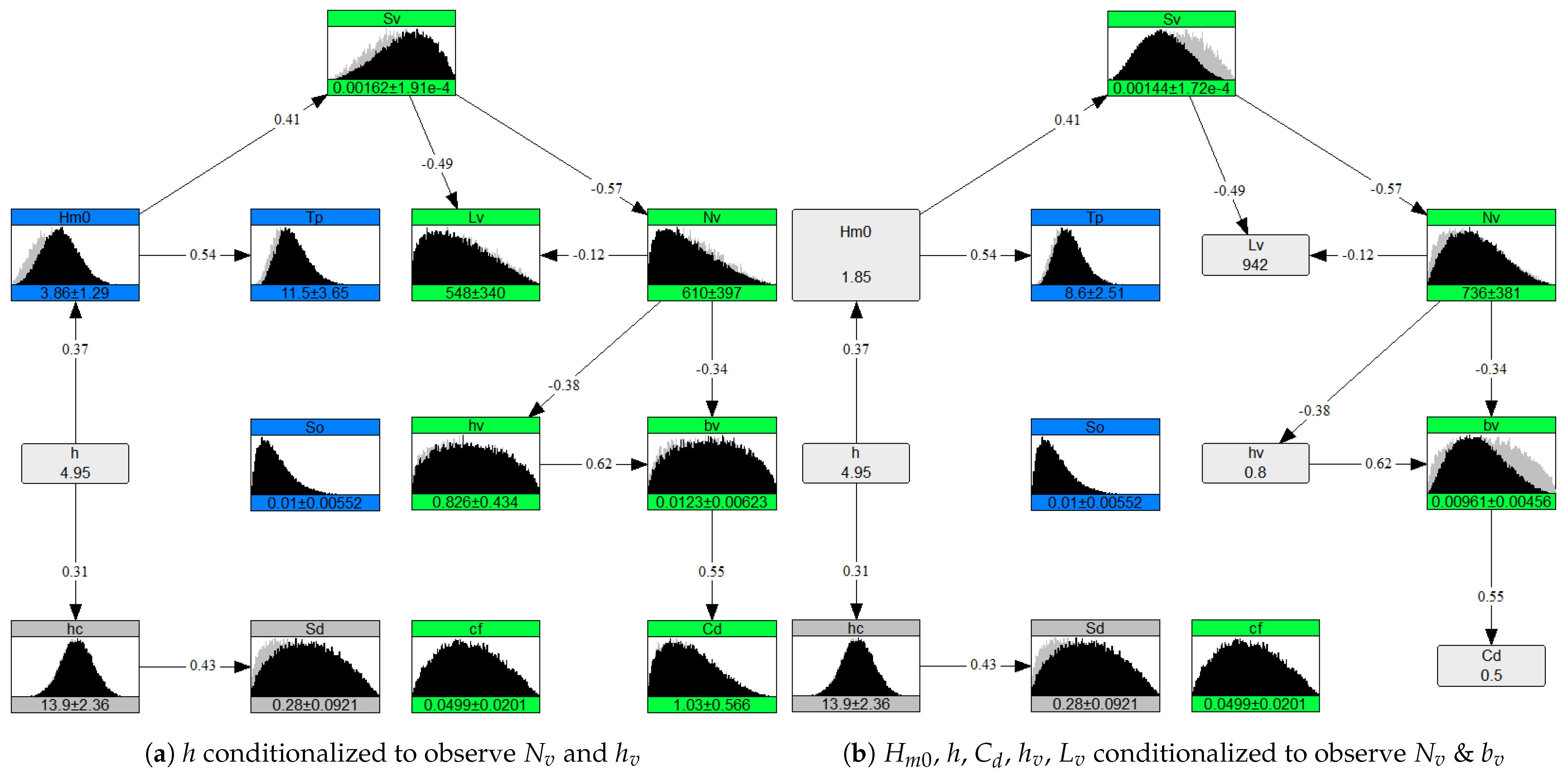
Measured data, especially for vegetation, still remains scarce, however this should not stop the attempts to understand biophysical systems and quantification of the value of nature-based solutions. While modeling such systems, these NPBNs could be used to extract missing information in data-scarce scenarios if all the boundary conditions are not available. The dependence modeling makes sure that the rest of the boundary conditions fall into physically realistic ranges. As an application, this has been illustrated in Figure 13b using the conditions measured for Posidonia oceanica species in the Mediterranean Sea by [39]. First, in Figure 13a only one variable h was conditionalized to observe other dependent variables in a highly data-scarce case. While some variables like $N_v=610$ stems/m${}^2$ and $h_v=0.826$ m were within less than 3% error range when compared to the measured ones $(N_v=615$ and $h_v=0.8)$, other variables provided fairly acceptable (but not very accurate) first-order estimates. Subsequently, more known variables were conditionalized to make the NPBN case specific. The NPBN was updated after conditionalizing $H_{m0}$, h, $C_d$, $h_v$, and $L_v$, and the mean values of $N_v=736$ stems/m${}^2$ and $b_v=0.0096$ m were observed. When compared to measured values of $N_v=615$ and $b_v=0.0086$ m by [39], the error was found to be within acceptable range (19% and 11% respectively). It is noteworthy that NPBNs provide an advantage to assimilate new information from newer sources in the existing model [91]. On the other hand, as argued by [92], for the optimal use of probabilistic models subject knowledge and physical understanding about the context of the modeler plays an important role.

4.1.4. Better System-Based Response

Thinking in terms of traditional sensitivity analysis, where one variable is varied while keeping all others fixed, the proposed method of conducting sensitivity analysis using correlated boundary conditions that vary all at once has an added advantage. As we believe natural systems are highly dynamic and often show nonlinear responses, the system response to boundary conditions that are varied individually would be comparatively different to the response generated by changing all boundary conditions simultaneously. Therefore, contrarily to the proposed method, traditional sensitivity analysis does not suffice in determining the real system response to varied conditions. Using dependence modeling to generate boundary conditions that vary all together but in a correlated way not only provides physically-realistic conditions but also adds value to any further analysis done using those conditions.

4.2. Limitations and Way forward

The limitations of this study are based on simplification choices and the restrictions of the tools used for modeling.

• Rigid Cylindrical Vegetation: Vegetation was modeled as rigid cylinders which do not bend, undergo uprooting, or break in storm conditions which are critical for the system response [85].
• Data Availability: Ideally the statistical description should be derived from the data but due to limited data and responses, stochastic modeling was performed using in-house expert judgment for some of the variables.
• Gaussian Copula: Dependence analysis throughout the study was based on Gaussian copula. However, there is evidence of other dependence structures [80] for the variables in this study.

Recommendations for improvement and future research direction are listed below.

• New field data or data from global models could be obtained to expand the domain and scale of hydrodynamic and vegetation variables both spatially and temporally.
• Better dependence structure, e.g., vines, could be explored since the Gaussian copula is not the most accurate dependence description for some of the variables.

As a way forward, the results from this study in the form of physically realistic vegetated hydrodynamic conditions could be utilized to carry out hydrovegetation numerical modeling. The aim here would be to observe generalized system response in terms of flood hazard reduction potential of vegetation under a variety of conditions. Variables such as the wave attenuation coefficient or run-up could be added to the existing NPBNs from this study to relate physical boundary conditions to the resulting effect of vegetation on hydrodynamics.

5. Conclusions

The vegetated hydrodynamic system was probabilistically parameterized using a range, distribution, and correlations among variables. The system was stochastically modeled using nonparametric Bayesian networks for sea grasses, salt marshes, and mangroves. The resulting NPBNs revealed dominant correlations among variables which derive the dynamics of the vegetated hydrodynamic system. NPBNs also revealed dependence information among variables beyond the pair-wise correlations which were initially quantified to set up the model. Modeling salt marsh and mangrove systems stochastically has enabled assessment of holistic system-based response to variations in individual variables. The NPBNs are capable of generating physically-realistic varied boundary conditions that are useful for further analysis such as reducing hydrovegetation numerical simulations required to acquire generalized information, improving traditional randomly-selected sensitivity analysis with a more cross-disciplinary system-based sensitivity analysis, and filling information in data-scarce environments. The main findings, which were derived by using a NPBN, help to pave the way for generating both generalized and predictive knowledge required for implementation of nature-based solutions in a range of realistic conditions that can be found across global coastal foreshores.

References

- Niazi, M.H.K.; Morales Nápoles, O.; van Wesenbeeck, B.K. Vegetated Hydrodynamic System: Parameterization and Stochastic Dependence Modelling. Coast. Eng. Proc. 2020. [Google Scholar] [CrossRef]
- Spalding, M.D.; McIvor, A.L.; Beck, M.W.; Koch, E.W.; Möller, I.; Reed, D.J.; Rubinoff, P.; Spencer, T.; Tolhurst, T.J.; Woodroffe, C.D.; et al. Coastal Ecosystems: A Critical Element of Risk Reduction. Conserv. Lett. 2014, 7, 293–301. [Google Scholar] [CrossRef]
- Niazi, M.H.K.; Sigalas, N.; Scott, F.; Grossmann, F.; Damdam, K. Robust Flood Defence in Response to Climate Change; Report; Delft University of Technology: Delft, The Netherlands, 2018. [Google Scholar]
- Carrick, J.; Abdul Rahim, M.S.A.B.; Adjei, C.; Ashraa Kalee, H.H.H.; Banks, S.J.; Bolam, F.C.; Campos Luna, I.M.; Clark, B.; Cowton, J.; Domingos, I.F.N.; et al. Is planting trees the solution to reducing flood risks? J. Flood Risk Manag. 2018, 12, e12484. [Google Scholar] [CrossRef] [Green Version]
- Fonseca, M.S.; Cahalan, J.A. A preliminary evaluation of wave attenuation by four species of seagrass. Estuarine Coast. Shelf Sci. 1992, 35, 565–576. [Google Scholar] [CrossRef]
- Kobayashi, N.; Raichle, A.W.; Asano, T. Wave Attenuation by Vegetation. J. Waterw. Port Coastal Ocean. Eng. 1993, 119, 30–48. [Google Scholar] [CrossRef]
- Paul, M.; Amos, C.L. Spatial and seasonal variation in wave attenuation over Zostera noltii. J. Geophys. Res. Ocean. 2011, 116. [Google Scholar] [CrossRef]
- Sánchez-González, J.F.; Sánchez-Rojas, V.; Memos, C.D. Wave attenuation due to Posidonia oceanica meadows. J. Hydraul. Res. 2011, 49, 503–514. [Google Scholar] [CrossRef]
- Horstman, E.M.; Dohmen-Janssen, C.M.; Narra, P.M.F.; van den Berg, N.J.F.; Siemerink, M.; Hulscher, S.J.M.H. Wave attenuation in mangroves: A quantitative approach to field observations. Coast. Eng. 2014, 94, 47–62. [Google Scholar] [CrossRef]
- Marsooli, R.; Wu, W. Numerical investigation of wave attenuation by vegetation using a 3D RANS model. Adv. Water Resour. 2014, 74, 245–257. [Google Scholar] [CrossRef]
- Möller, I.; Kudella, M.; Rupprecht, F.; Spencer, T.; Paul, M.; van Wesenbeeck, B.K.; Wolters, G.; Jensen, K.; Bouma, T.J.; Miranda-Lange, M.; et al. Wave attenuation over coastal salt marshes under storm surge conditions. Nat. Geosci. 2014, 7, 727. [Google Scholar] [CrossRef] [Green Version]
- Van Rooijen, A.A.; De Vries, J.S.M.V.T.; Mccall, R.T.; Van Dongeren, A.R.; Roelvink, J.A.; Reniers, A.J.H.M. Modeling of Wave Attenuation by Vegetation with Xbeach. In Proceedings of the 36th Iahr World Congress, The Hague, The Netherlands, 28 June–3 July 2015; pp. 6749–6755. [Google Scholar]
- Vuik, V.; Jonkman, S.N.; Borsje, B.W.; Suzuki, T. Nature-based flood protection: The efficiency of vegetated foreshores for reducing wave loads on coastal dikes. Coast. Eng. 2016, 116, 42–56. [Google Scholar] [CrossRef] [Green Version]
- Reidenbach, M.A.; Thomas, E.L. Influence of the Seagrass, Zostera marina, on Wave Attenuation and Bed Shear Stress Within a Shallow Coastal Bay. Front. Mar. Sci. 2018, 5. [Google Scholar] [CrossRef]
- Mattis, S.A.; Kees, C.E.; Wei, M.V.; Dimakopoulos, A.; Dawson, C.N. Computational Model for Wave Attenuation by Flexible Vegetation. J. Waterw. Port Coastal Ocean. Eng. 2019, 145, 04018033. [Google Scholar] [CrossRef]
- Montgomery, J.M.; Bryan, K.R.; Mullarney, J.C.; Horstman, E.M. Attenuation of Storm Surges by Coastal Mangroves. Geophys. Res. Lett. 2019, 46, 2680–2689. [Google Scholar] [CrossRef] [Green Version]
- Phan, K.L.; Stive, M.J.F.; Zijlema, M.; Truong, H.S.; Aarninkhof, S.G.J. The effects of wave non-linearity on wave attenuation by vegetation. Coast. Eng. 2019, 147, 63–74. [Google Scholar] [CrossRef]
- Wu, W.C.; Ma, G.; Cox, D.T. Modeling wave attenuation induced by the vertical density variations of vegetation. Coast. Eng. 2016, 112, 17–27. [Google Scholar] [CrossRef]
- Karambas, T.; Koftis, T.; Prinos, P. Modeling of Nonlinear Wave Attenuation due to Vegetation. J. Coast. Res. 2016, 32, 142–152. [Google Scholar]
- Maza, M.; Lara, J.L.; Losada, I.J. Solitary wave attenuation by vegetation patches. Adv. Water Resour. 2016, 98, 159–172. [Google Scholar] [CrossRef]
- Chu, P.C.; Kuo, Y.; Galanis, G. Statistical Structure of the Global Significant Wave Heights. In Proceedings of the 20th Conference on Probability and Statistics in the Atmospheric Sciences, Atlanta, GA, USA, 16–21 January 2010. [Google Scholar]
- Xu, D.; Li, X.; Zhang, L.; Xu, N.; Lu, H. On the distributions of wave periods, wavelengths, and amplitudes in a random wave field. J. Geophys. Res. Ocean. 2004, 109. [Google Scholar] [CrossRef]
- Hawkes, P.J.; Gouldby, B.P.; Tawn, J.A.; Owen, M.W. The joint probability of waves and water levels in coastal engineering design. J. Hydraul. Res. 2002, 40, 241–251. [Google Scholar] [CrossRef]
- Guedes Soares, C.; Carvalho, A.N. Probability distributions of wave heights and periods in combined sea-states measured off the Spanish coast. Ocean. Eng. 2012, 52, 13–21. [Google Scholar] [CrossRef]
- Muraleedharan, G.; Lucas, C.; Martins, D.; Guedes Soares, C.; Kurup, P.G. On the distribution of significant wave height and associated peak periods. Coast. Eng. 2015, 103, 42–51. [Google Scholar] [CrossRef]
- Hu, Z.; Stive, M.; Zitman, T.; Suzuki, T. Drag coefficient of vegetation in flow modeling. In Proceedings of the International Conference on Coastal Engineering, Santander, Spain, 1–6 July 2012. [Google Scholar] [CrossRef] [Green Version]
- Simard, M.; Fatoyinbo, L.; Smetanka, C.; Rivera-Monroy, V.H.; Castañeda-Moya, E.; Thomas, N.; Van der Stocken, T. Mangrove canopy height globally related to precipitation, temperature and cyclone frequency. Nat. Geosci. 2019, 12, 40–45. [Google Scholar] [CrossRef]
- Reimann, S.; Husrin, S.; Strusińska, A.; Oumeraci, H. Damping Tsunami And Storm Waves By Coastal Forests – Parameterisation And Hydraulic Model Tests; Leibniz University Hannover: Hannover, Germany, 2019. [Google Scholar]
- Athanasiou, P.; van Dongeren, A.; Giardino, A.; Vousdoukas, M.; Gaytan-Aguilar, S.; Ranasinghe, R. Global distribution of nearshore slopes with implications for coastal retreat. Earth Syst. Sci. Data 2019, 11, 1515–1529. [Google Scholar] [CrossRef] [Green Version]
- Niazi, M.H.K. Flood Risk Prediction under Global Vegetated Hydrodynamics: A Bayesian Network. MSc Thesis, Delft University of Technology, Delft, The Netherlands, 2019. [Google Scholar]
- van Zelst, V. Global Flood Hazard Reduction by Foreshore Vegetation. MSc Thesis, Delft University of Technology, Delft, The Netherlands, 2018. [Google Scholar]
- Chen, H.; Ni, Y.; Li, Y.; Liu, F.; Ou, S.; Su, M.; Peng, Y.; Hu, Z.; Uijttewaal, W.; Suzuki, T. Deriving vegetation drag coefficients in combined wave-current flows by calibration and direct measurement methods. Adv. Water Resour. 2018, 122, 217–227. [Google Scholar] [CrossRef] [Green Version]
- Henry, P.Y.; Myrhaug, D.; Aberle, J. Drag forces on aquatic plants in nonlinear random waves plus current. Estuarine Coast. Shelf Sci. 2015, 165, 10–24. [Google Scholar] [CrossRef]
- Asano, T.; Tsutsui, S.; Sakai, T. Wave damping characteristics due to seaweed. In Proceedings of the 35th Conference on Coastal Engineering, Kobe, Japan, 7 November 1988. [Google Scholar]
- Méndez, F.J.; Losada, I.J.; Losada, M.A. Hydrodynamics induced by wind waves in a vegetation field. J. Geophys. Res. Ocean. 1999, 104, 18383–18396. [Google Scholar] [CrossRef]
- Mendez, F.J.; Losada, I.J. An empirical model to estimate the propagation of random breaking and nonbreaking waves over vegetation fields. Coast. Eng. 2004, 51, 103–118. [Google Scholar] [CrossRef]
- Bradley, K.; Houser, C. Relative velocity of seagrass blades: Implications for wave attenuation in low-energy environments. J. Geophys. Res. Earth Surf. 2009, 114. [Google Scholar] [CrossRef]
- Jadhav, R.S.; Chen, Q. Field Investigation of Wave Dissipation Over SaltMarsh Vegetation During Tropical Cyclone. In Proceedings of the 33rd Conference on Coastal Engineering, Santander, Spain, 1–6 July 2012. [Google Scholar] [CrossRef] [Green Version]
- Infantes, E.; Orfila, A.; Simarro, G.; Terrados, J.; Luhar, M.; Nepf, H. Effect of a seagrass (Posidonia oceanica) meadow on wave propagation. Mar. Ecol. Prog. Ser. 2012, 456, 63–72. [Google Scholar] [CrossRef] [Green Version]
- Jadhav, R.S.; Chen, Q.; Smith, J.M. Spectral distribution of wave energy dissipation by salt marsh vegetation. Coast. Eng. 2013, 77, 99–107. [Google Scholar] [CrossRef] [Green Version]
- Pinsky, M.L.; Guannel, G.; Arkema, K.K. Quantifying wave attenuation to inform coastal habitat conservation. Ecosphere 2013, 4, art95. [Google Scholar] [CrossRef]
- Maza, M.; Lara, J.L.; Losada, I.J. A coupled model of submerged vegetation under oscillatory flow using Navier–Stokes equations. Coast. Eng. 2013, 80, 16–34. [Google Scholar] [CrossRef]
- Ozeren, Y.; Wren, D.G.; Wu, W. Experimental Investigation of Wave Attenuation through Model and Live Vegetation. J. Waterw. Port Coast. Ocean. Eng. 2014, 140. [Google Scholar] [CrossRef]
- Anderson, M.E.; Smith, J.M. Wave attenuation by flexible, idealized salt marsh vegetation. Coast. Eng. 2014, 83, 82–92. [Google Scholar] [CrossRef]
- Hu, Z.; Suzuki, T.; Zitman, T.; Uittewaal, W.; Stive, M. Laboratory study on wave dissipation by vegetation in combined current–wave flow. Coast. Eng. 2014, 88, 131–142. [Google Scholar] [CrossRef]
- Losada, I.J.; Maza, M.; Lara, J.L. A new formulation for vegetation-induced damping under combined waves and currents. Coast. Eng. 2016, 107, 1–13. [Google Scholar] [CrossRef]
- Plomaritis, T.A.; Costas, S.; Ferreira, Ó. Use of a Bayesian Network for coastal hazards, impact and disaster risk reduction assessment at a coastal barrier (Ria Formosa, Portugal). Coast. Eng. 2018, 134, 134–147. [Google Scholar] [CrossRef]
- Narayan, S.; Simmonds, D.; Nicholls, R.J.; Clarke, D. A Bayesian network model for assessments of coastal inundation pathways and probabilities. J. Flood Risk Manag. 2018, 11, S233–S250. [Google Scholar] [CrossRef]
- Jäger, W.S.; Christie, E.K.; Hanea, A.M.; den Heijer, C.; Spencer, T. A Bayesian network approach for coastal risk analysis and decision making. Coast. Eng. 2018, 134, 48–61. [Google Scholar] [CrossRef]
- Bolle, A.; das Neves, L.; Smets, S.; Mollaert, J.; Buitrago, S. An impact-oriented Early Warning and Bayesian-based Decision Support System for flood risks in Zeebrugge harbour. Coast. Eng. 2018, 134, 191–202. [Google Scholar] [CrossRef]
- Pearson, S.G.; Storlazzi, C.D.; van Dongeren, A.R.; Tissier, M.F.S.; Reniers, A.J.H.M. A Bayesian-Based System to Assess Wave-Driven Flooding Hazards on Coral Reef-Lined Coasts. J. Geophys. Res. Ocean. 2017, 122, 10099–10117. [Google Scholar] [CrossRef] [Green Version]
- Poelhekke, L.; Jäger, W.S.; van Dongeren, A.; Plomaritis, T.A.; McCall, R.; Ferreira, Ó. Predicting coastal hazards for sandy coasts with a Bayesian Network. Coast. Eng. 2016, 118, 21–34. [Google Scholar] [CrossRef]
- Den Heijer, C.; Knipping, D.T.J.A.; Plant, N.G.; Van Thiel De Vries, J.S.M.; Baart, F.; Van Gelder, P.H.A.J.M. Impact assessment of extreme storm events using a Bayesian network. Conf. Coast. Eng. 2012, 33, 4. [Google Scholar] [CrossRef] [Green Version]
- Plant, N.G.; Holland, K.T. Prediction and assimilation of surf-zone processes using a Bayesian network: Part I: Forward models. Coast. Eng. 2011, 58, 119–130. [Google Scholar] [CrossRef]
- Kurowicka, D.; Cooke, R. Non-Parametric Continuous Bayesian Belief Nets with Expert Judgement. Probab. Saf. Assess. Manag. 2004, 2784–2790. [Google Scholar]
- Hanea, A.M.; Kurowicka, D.; Cooke, R.M. Hybrid Method for Quantifying and Analyzing Bayesian Belief Nets. Qual. Reliab. Eng. Int. 2006, 22, 709–729. [Google Scholar] [CrossRef]
- Ababei, D.; Lewandowski, D.; Hanea, A.; Napoles, O.M.; Kurowicka, D.; Cooke, R. UNINET Help Documentation; Report; Delft University of Technology: Delft, The Netherlands, 2008. [Google Scholar]
- Morales Napoles, O.; Worm, D.; Haak, P.v.d.; Hanea, A.; Courage, W.; Miraglia, S. Reader for Course: Introduction to Bayesian Networks; Report; Netherlands Organisation for Applied Scientific Research: Delft, The Netherlands, 2013. [Google Scholar]
- Hanea, A.; Morales Napoles, O.; Ababei, D. Non-parametric Bayesian networks: Improving theory and reviewing applications. Reliab. Eng. Syst. Saf. 2015, 144, 265–284. [Google Scholar] [CrossRef]
- Genest, C.; Mackay, J. The Joy of Copulas: Bivariate Distributions with Uniform Marginals. Am. Stat. 1986, 40, 280–283. [Google Scholar] [CrossRef]
- Frees, E.W.; Valdez, E.A. Understanding Relationships Using Copulas. North Am. Actuar. J. 1998, 2, 1–25. [Google Scholar] [CrossRef]
- Genest, C.; Favre, A.C. Everything you always wanted to know about copula modeling but were afraid to ask. J. Hydrol. Eng. 2007, 12, 347–368. [Google Scholar] [CrossRef]
- Schweizer, B. Introduction to copulas. J. Hydrol. Eng. 2007, 12, 346. [Google Scholar] [CrossRef] [Green Version]
- Yule, G.U. An Introduction to the Theory of Statistics; Griffin, C., Ed.; Limited: London, UK, 1919. [Google Scholar]
- Songy, G. Wave Attenuation by Global Coastal Salt Marsh Habitats. MSc Thesis, Delft University of Technology, Delft, The Netherlands, 2016. [Google Scholar]
- Holthuijsen, L.H. Waves in oceanic and coastal waters; Cambridge University Press: Cambridge, UK, 2010. [Google Scholar]
- Young, I.R.; Zieger, S.; Babanin, A.V. Global Trends in Wind Speed and Wave Height. Science 2011, 332, 451. [Google Scholar] [CrossRef] [PubMed]
- Young, I.R. Global ocean wave statistics obtained from satellite observations. Appl. Ocean. Res. 1994, 16, 235–248. [Google Scholar] [CrossRef]
- Janssen, M. Flood Hazard Reduction by Mangroves. Msc Thesis, Delft University of Technology, Delft, The Netherlands, 2016. [Google Scholar]
- Rahmeyer, W.; Werth, D. The Study of the Resistance and Stability of Vegetation Ecosystem Plant Groupings in Flood Control Channels; Report 148; UtahState Univeristy: Logan, UT, USA, 1996; Volume 1. [Google Scholar]
- Chow, V.T. Open-Channel Hydraulics; McGraw-Hill: New York, NY, USA, 1959; Volume 1. [Google Scholar]
- CIRIA; CUR; CETMEF. The Rock Manual. The Use of Rock in Hydraulic Engineering, 2nd ed.; C683; CIRIA: London, UK, 2007. [Google Scholar]
- Marek, P. Mangroves. 2019. Available online: www.mangrove.at (accessed on 15 July 2019).
- Moffett, K.B.; Nardin, W.; Silvestri, S.; Wang, C.; Temmerman, S. Multiple Stable States and Catastrophic Shifts in Coastal Wetlands: Progress, Challenges, and Opportunities in Validating Theory Using Remote Sensing and Other Methods. Remote Sens. 2015, 7, 10184–10226. [Google Scholar] [CrossRef] [Green Version]
- Cooke, R. Experts in Uncertainty: Opinion and Subjective Probability in Science; Oxford University Press on Demand: Oxford, UK, 1991. [Google Scholar]
- Morales Napoles, O.; Kurowicka, D.; Roelen, A. Eliciting conditional and unconditional rank correlations from conditional probabilities. Reliab. Eng. Syst. Saf. 2008, 93, 699–710. [Google Scholar] [CrossRef]
- Cooke, R.M.; Goossens, L.L.H.J. TU Delft expert judgment data base. Reliab. Eng. Syst. Saf. 2008, 93, 657–674. [Google Scholar] [CrossRef]
- Morales-Nápoles, O.; Delgado-Hernández, D.J.; De-León-Escobedo, D.; Arteaga-Arcos, J.C. A continuous Bayesian network for earth dams’ risk assessment: Methodology and quantification. Struct. Infrastruct. Eng. 2014, 10, 589–603. [Google Scholar] [CrossRef]
- Werner, C.; Bedford, T.; Cooke, R.M.; Hanea, A.M.; Morales-Nápoles, O. Expert judgement for dependence in probabilistic modelling: A systematic literature review and future research directions. Eur. J. Oper. Res. 2017, 258, 801–819. [Google Scholar] [CrossRef] [Green Version]
- Jäger, W.S.; Nápoles, O.M. A Vine-Copula Model for Time Series of Significant Wave Heights and Mean Zero-Crossing Periods in the North Sea. ASCE-ASME J. Risk Uncertain. Eng. Syst. Part Civ. Eng. 2017, 3, 04017014. [Google Scholar] [CrossRef] [Green Version]
- Rodríguez, G.R.; Guedes Soares, C. Correlation between successive wave heights and periods in mixed sea states. Ocean. Eng. 2001, 28, 1009–1030. [Google Scholar] [CrossRef]
- Antão, E.M.; Guedes Soares, C. Joint distributions of wave steepness in narrow band sea states. Ocean. Eng. 2015, 101, 201–210. [Google Scholar] [CrossRef]
- Memos, C.D. On the theory of the joint probability of heights and periods of sea waves. Coast. Eng. 1994, 22, 201–215. [Google Scholar] [CrossRef]
- Longuet-Higgins, M.S. On the joint distribution of the periods and amplitudes of sea waves. J. Geophys. Res. 1975, 80, 2688–2694. [Google Scholar] [CrossRef]
- Vuik, V.; Suh Heo, H.Y.; Zhu, Z.; Borsje, B.W.; Jonkman, S.N. Stem breakage of salt marsh vegetation under wave forcing: A field and model study. Estuarine Coast. Shelf Sci. 2018, 200, 41–58. [Google Scholar] [CrossRef] [Green Version]
- Terefenko, P.; Paprotny, D.; Giza, A.; Morales-Nápoles, O.; Kubicki, A.; Walczakiewicz, S. Monitoring Cliff Erosion with LiDAR Surveys and Bayesian Network-based Data Analysis. Remote Sens. 2019, 11, 843. [Google Scholar] [CrossRef] [Green Version]
- Mendoza-Lugo, M.A.; Delgado-Hernández, D.J.; Morales-Nápoles, O. Reliability analysis of reinforced concrete vehicle bridges columns using non-parametric Bayesian networks. Eng. Struct. 2019, 188, 178–187. [Google Scholar] [CrossRef]
- Lee, D.; Pan, R. A nonparametric Bayesian network approach to assessing system reliability at early design stages. Reliab. Eng. Syst. Saf. 2018, 171, 57–66. [Google Scholar] [CrossRef]
- Couasnon, A.; Sebastian, A.; Morales-Nápoles, O. A Copula-Based Bayesian Network for Modeling Compound Flood Hazard from Riverine and Coastal Interactions at the Catchment Scale: An Application to the Houston Ship Channel, Texas. Water 2018, 10, 1190. [Google Scholar]
- Pearson, S. Predicting Wave-Induced Flooding on Low-Lying Tropical Islands Using a Bayesian Network. MSc Thesis, Delft University of Technology, Delft, The Netherlands, 2016. [Google Scholar]
- Han, S.; Coulibaly, P. Bayesian flood forecasting methods: A review. J. Hydrol. 2017, 551, 340–351. [Google Scholar] [CrossRef]
- Jaeger, W. Multivariate Methods for Coastal and Offshore Risks. Ph.D. Thesis, Delft University of Technology, Delft, The Netherlands, 2018. [Google Scholar]
Figure 1.
Hybrid and nature-based solutions in the hierarchy of flood defenses. Both conventional and nature-based solutions complement each other in the design of robust hybrid flood defenses.
Figure 2.
Overall methodology and steps for stochastic modeling in UNINET.
Figure 3.
Idealized profile used for stochastic modeling including six segments with distinct hydrodynamic and vegetation characteristics.
Figure 4.
Vegetation schematization: benthic vegetation (seagrasses) as bottom friction, submerged vegetation (saltmarshes) as rigid cylinders and emergent (mangroves) as rigid cylinder with 3 vertical layer schematizations. See nomenclature in appendices for variables’ explanation.
Figure 5.
Idealized vegetated hydrodynamic system for stochastic modeling. See nomenclature in appendices for variables’ explanation.
Figure 6.
Copula and correlations from field data for vegetation height and frontal width .
Figure 7.
Copulas and correlations determined from data for hydrodynamic variables .
Figure 10.
Correlations in global vegetated hydrodynamic conditions in saltmarshes (a,b) and mangroves (c,d). The circles represent nodes (variables), lines represent the correlations in the network, and thickness of the lines represents strength of the correlation. Plots (b) and (d) have minimum correlation threshold of 0.1 to distinguish dominant correlations.
Figure 11.
Sampled profiles (10/300).
Figure 12.
Comparison of varied vegetated hydrodynamic conditions sampled from an independent DAG with uniformly distributed variables (gray dots) and the stochastic model of this study (black dots) that was quantified with distributions (Table 2) and correlations (Table 4). Yellow panels shows the distinct sampling of the variable pair with positive and negative dependence .
Figure 13.
Case application using the conditions measured by [39].