
Clustering Simultaneous Occurrences of the Extreme Floods in the Neckar Catchment


Department of Hydrology and Geohydrology, Institute for Water and Environmental System Modeling—IWS, University of Stuttgart, 70569 Stuttgart, Germany
*
Author to whom correspondence should be addressed.
Water 2021, 13(4), 399; https://doi.org/10.3390/w13040399
Submission received: 27 December 2020
/
Revised: 19 January 2021
/
Accepted: 1 February 2021
/
Published: 4 February 2021
(This article belongs to the Special Issue Stochastic Modelling of Hydrometeorological Processes for Engineering Applications)
Abstract
:Flood protection is crucial for making socioeconomic policies due to the high losses of extreme floods. So far, the synchronous occurrences of flood events have not been deeply investigated. In this paper, multivariate analysis was implemented to reveal the interconnection between these floods in spatiotemporal resolution. The discharge measurements of 46 gauges with a continuous daily time series for 55 years were taken over the Neckar catchment. Initially, the simultaneous floods were identified. The Kendall correlation between the pair sets of peaks was determined to scrutinize the similarities between the simultaneous events. Agglomerative hierarchical clustering tree (AHCT) and multidimensional scaling (MDS) were employed, and obtained clusters were compared and evaluated with the Silhouette verification method. AHCT shows that the Average and Ward algorithms are appropriate to detect reasonable clusters. The Neckar catchment has been divided into three major clusters: the first cluster mainly covers the western part and is bounded by the Black Forest and Swabian Alps. The second cluster is mostly located in the eastern part of the upper Neckar. The third cluster contains the remaining lowland areas of the Neckar basin. The results illustrate that the clusters act relatively as a function of topography, geology, and anthropogenic alterations of the catchment.
1. Introduction
Floods are considered one of the utmost devastating natural disasters in the world. Approximately one billion people around the world are living in floodplains [1]. In Europe, these extreme events have led to more than 426 billion euros of loss between 1980–2017 [2]. Particularly, in Germany, two catastrophic floods happened in 2002 and 2013, which caused damage over 26 billion dollars [3]. Additionally, in 2016, the loss was estimated to be 4.1 billion dollars due to a couple of extreme events in this area [4,5]. Traditionally, researchers were trying to find and identify the flood types and patterns which newly become visible that flood patterns have been changed in terms of magnitude and timing due to climate change [6,7,8,9,10,11]. Blöschl et al. [9] detected noticeable patterns of flood timing shift over European countries for the last fifty years.
Likewise, flood risk assessment and subsequently, flood control requires precise statistical analyses in terms of precipitation and runoff for insurance purposes or the design of appropriate flood monitoring systems [12]. Flood defenses are critical components when they come to flood hazards. The flood risk changes are irregularly distributed, with the most substantial increases in Asia, the USA, and Europe [13]. It is substantial to deal accurately with their effect and consider the concurrency of flood occurrences. After the 2002 flood event, which caused colossal destructions in the Elbe and Danube catchments, the existing German water and planning regulations were subjected to several modifications [14]. Before the catastrophic flood in 2013, many of the problems are recognized due to the last immense flood and put into action. However, other overwhelming events in 2013 and 2016 showed that the simultaneous events were not still considered in the regular frequency and magnitude analysis. Besides, the discharge waves in various river catchments might be interconnected to a unique atmospheric event in a continental-scale analysis, enhancing the vulnerability level in risk [15]. Therefore, an unprecedented challenge still remains for accurately quantifying the potential flood damages. The floods that simultaneously affect many sites are critical topics in flood disaster management, as well as the indemnification for losses. Moreover, so far, risk map developers have not taken the simultaneous occurrences of extremes into account, which play a significant role in flood generating mechanisms, and the triggering system [16].
This study focuses on the Spatio-temporal multivariate analysis of extreme flood events, overcoming some univariate analysis disadvantages. The univariate flood frequency analysis is broadly used in hydrological studies focusing on analyzing flood peaks or flood volume [17,18,19]. Nevertheless, univariate statistics cannot discover the flood spatial interactions within catchments and neglects the combined effects of flood triggering factors and the probability of occurrence [20]. The peak points, primary behavior, and flood dynamics are required as the main properties for every fundamental analysis. Furthermore, in the multivariate spatiotemporal analysis, additional elements can be taken into account. However, multivariate analysis of such variables is rarely performed in this issue because the minimal available number of multivariate models are not well suited to represent extreme values [21]. The limit approaches are appropriate when all variables’ extreme values are unlikely to occur together or when the interest supports the joint distribution where only some subsets of components are extremes. The recent developments in multivariate extreme value methods opened opportunities for improving flood risk analysis methods [20,22,23,24,25]. Also, Falter et al. [26] proposed a novel approach innovatively evaluating river flood risk by considering magnitudes of peak discharge. However, still, the concurrency of floods was not assessed in their work.
Spatiotemporal clustering of floods may have considerable consequences for flood defense, design and risk management [27,28] and clustering of catastrophic events is an essential issue for the insurance and reinsurance industry to find a coefficient for different vulnerability zones [29]. So far, temporal clustering of some extreme hydrometeorological parameters is done. Villarini et al. [30] clustered the teleconnection pattern of floods and climate in the USA. Storms and cyclones were also clustered, which can be a triggering factor for extreme floods [31,32]. Flood clustering is reported in some new research [28,33,34,35,36,37], but they mainly worked on extreme floods and some rare research is assessed the simultaneous floods [38], which is a flood risks clustering based on hazard scenarios.
The proposed research aims to investigate the coincidence occurrence of flood events. In this paper, we address the following questions: 1. To what extent the simultaneous floods happened in the Neckar catchment? 2. What is the best hierarchical clustering linkage method to investigate simultaneously occurrences of floods? 3. How is the comparison between the clustered area by employing different clustering methods? Moreover, we assess the possibility of improving the current hydrological models to perform better on the extreme values based on newly proposed clusters of extremes. To answer these questions, we select discharge times series from 46 gauges in the Neckar basin. To identify the simultaneous floods, the two independent peaks per year are selected; however, there are some other standard methods like Peak Over Threshold (POT) [28,39,40]. The two methods of clustering are applied with two dissimilarity matrix to evaluate the functionality of different dissimilarities. Also, five linkage methods are employed to catch clustering maps with different design purposes.
2. Data and Case Study
2.1. Data
Daily discharge time series in this contribution for 46 subcatchments of the Neckar were obtained from the State Institute for the Environment Baden-Württemberg (LUBW) [41]. Also, daily precipitation time series of corresponding subcatchments were taken from “Deutsche Wetterdienst” (DWD) [42] to use only as a reference for identifying independent flood events in a year. The time series are span the time interval from 1961 to 2015. Subsequently, the time series with missing values were infilled by employing the spatial Copula-based interpolation [43].
2.2. Case Study
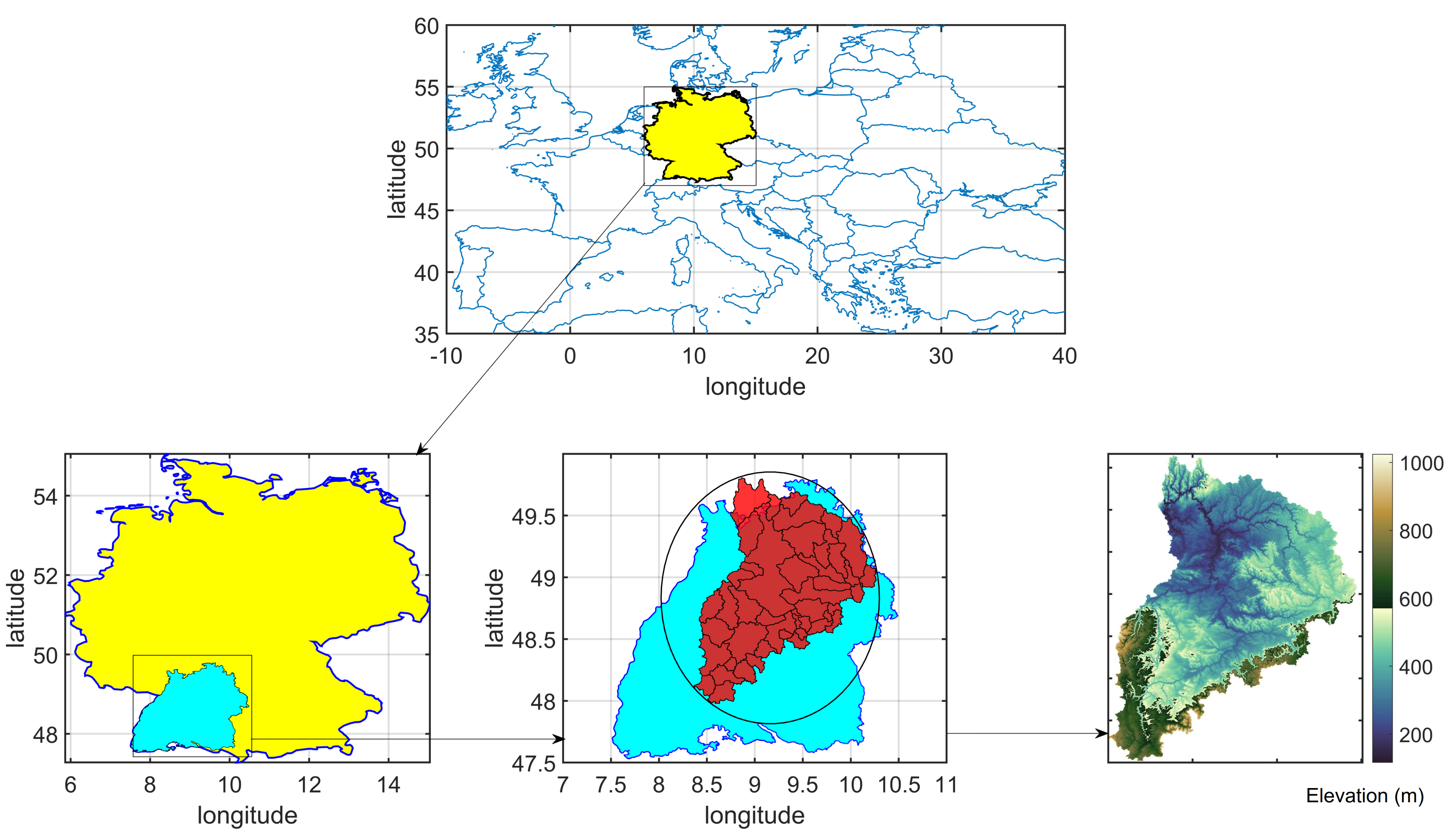
The Neckar catchment is located in the southwest of Germany and mostly in Baden Württemberg state. The Neckar is a tributary of the Rhine river, which is passes through four countries in Europe. The catchment area is approximately 14,000 km. The study was also carried out in 46 subcatchments with various drainage sizes from 60 to 14,000 km. The catchment elevation range is between 97 and 851 m. According to the lower right part of Figure 1, which shows the topographical altitude of the catchment, the highest elevation is in the southern and southwestern of the catchment near the Black Forest. Almost half of the subcatchments are located in the upper Neckar, which shows a higher concentration of the subcatchments due to high elevation regions. Furthermore, the length of the river Neckar is 367 km. This catchment covers around of the state’s area. The most important territories are Enz (2223 km), Kocher (1989 km), and Jagst (1837 km), then Nagold, Rems, and Fils are another branch of the river. Also, in terms of discharge volume and rainfall distribution, the river Neckar contributes on average 135 m. The local topography particularly adjusts the precipitation in the region. The highest mean annual precipitation value of 2000 mm recorded in the northern Black Forest, which is located in the mountainous part of the basin [44,45]. Towards the eastern part of the study area, the mean annual precipitation slim down to around 800–1000 mm [46]. Besides, the most extensive daily precipitation record among selected stations is 97 mm.
In terms of geology, this area can be categorized into nine central units, six of which are freshwater aquifers. Also, the non-permeable crystalline rock was specified as the bottom of the Neckar aquifer system [47]. The Neckar basin’s geological structure is characterized by a gentle dipping of the formations towards the southeast. The dipping layers lead to a complex hydrogeological condition; accordingly, the uppermost aquifer is formed by varying geological formations in distinct regions of the basin. In this situation, the hydrogeology of the basin is exceptionally complex [48]. Moreover, some anthropogenic changes affect the river and the consequent discharge in the research area’s independent tributaries. Kalweit et al. [49] and Bormann [50] mentioned that in the Neckar catchments, 60 reservoirs were constructed.
3. Methodology
3.1. Flood Events Identification
In this paper, the two biggest events per year for 55 years were selected for each location. These two events have to be independent of each other (). It means the second biggest peak should not be in ten-days intervals of the highest discharge in a year. Furthermore, each peak should result from an individual rainfall event (not the accumulation of complementary precipitation events in a period of ±10 days).
where and are two biggest independent maximums in the ith year and and are the day indices of their occurrences in that year.
3.2. Simultaneous Events and Their Corresponding Peaks
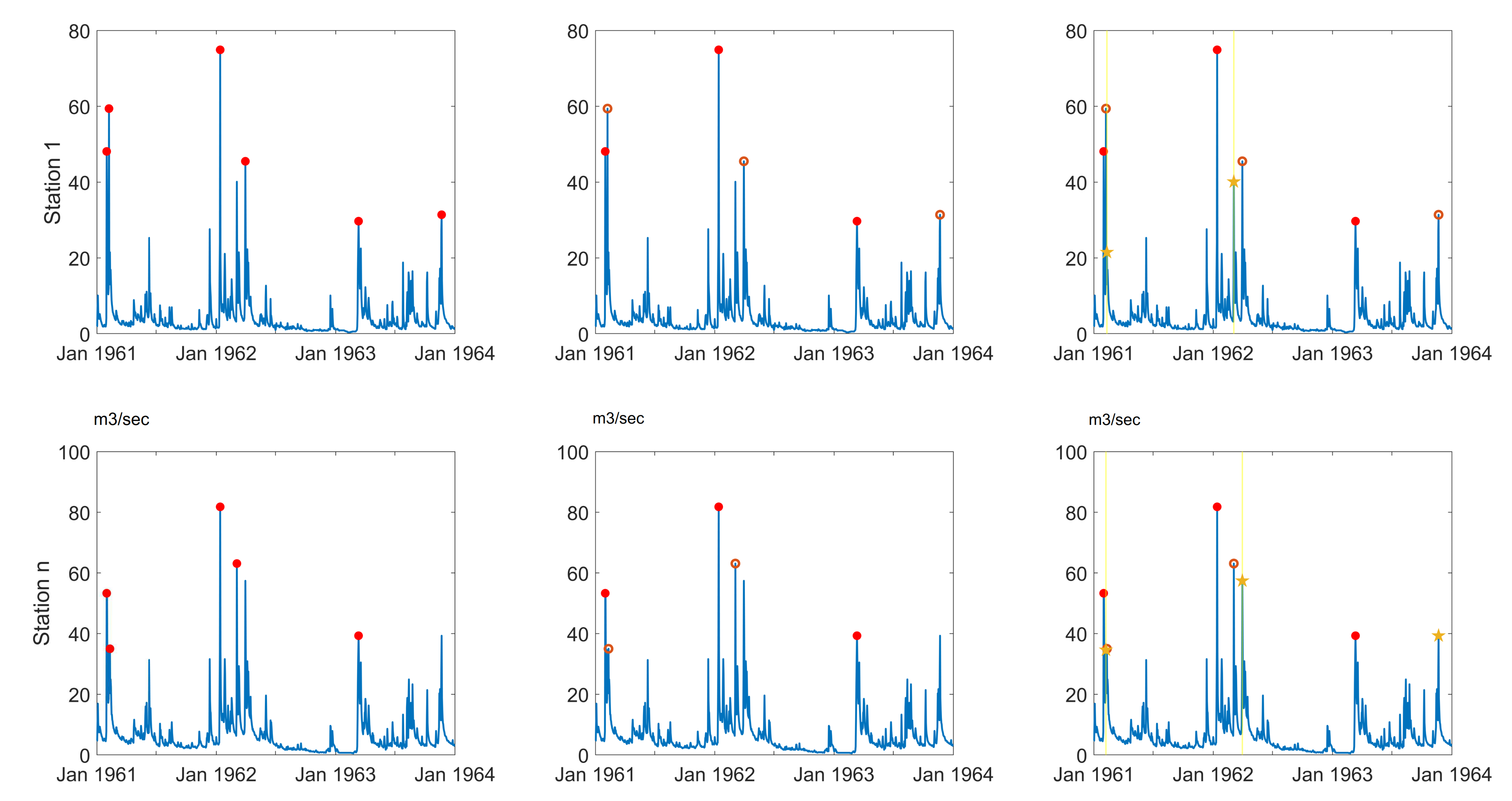
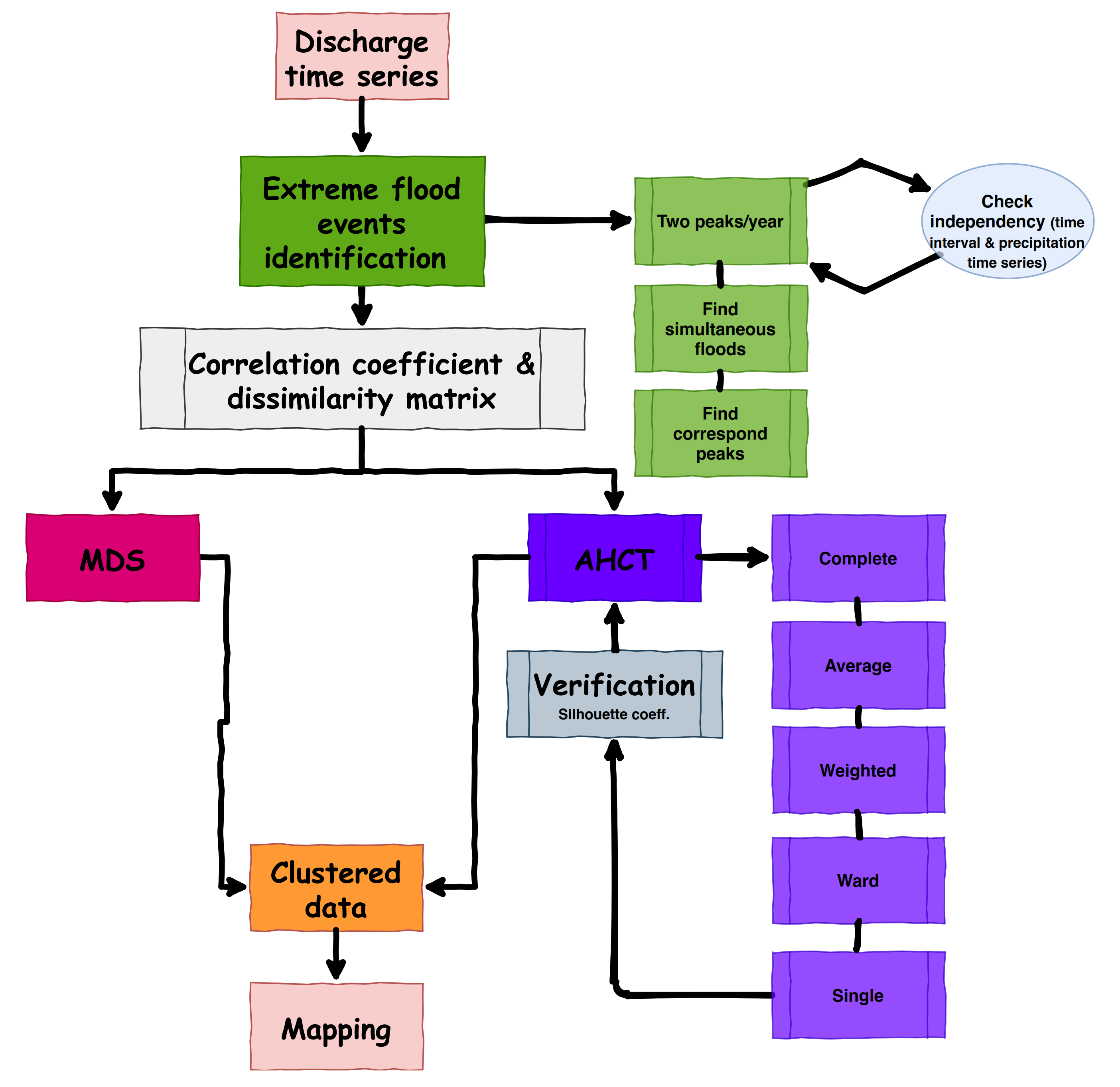
Identifying the flood events indicates the actual possible floods which occurred in the past decades. However, some extremes happened distinctly in terms of timing. To find the simultaneous occurrences, two days before and after each incident has been selected. If there is a peak in one station and in another is not, the corresponding peak in the time interval has been found. This procedure lets us not neglect any of these highest values and keep all possible information about the extreme event. The stepwise procedure is shown in Figure 2.
In Figure 2, as an example, the years between 1961 and 1964 were demonstrated. The upper figures belong to the first station, and the lower figures are for a random station. Two left figures show the identified events independently in this year in red dots. Some of the events happened at the same time (within two days interval), and some individually took place. In the middle, individual events were displayed by a red circle. These circles are the events that independently occurred in this period of time. The figures (right panel) illustrate the corresponding discharge (with the star shape symbol) of each individual event (red circles). The highlighted yellow bound is a time window in which the corresponding discharge is the highest value in this boundary.
3.3. Investigation of Associations among Simultaneous Flood Series and Distance Matrix
Every two measurement stations have a pair set of coinciding extremes, which can have a minimum of 110 pairs of peaks (it means two peaks per year for each discharge gauge). The minimum status can arise when all flood occasions happened at the same time and be synchronized. Furthermore, 220 pairs would be a maximum range, thus point to a lack of coincidence floods in the two series of peaks. To find the similarity of the data orderings when ranked by each of the quantities, Kendall’s Tau correlation of each pair was calculated, and the square correlation matrix was achieved. The distance matrix to clarify the discrepancies among stations was evaluated with two different methods regarding this matrix. The first method is Kendall, and the second is the Euclidean distance. The flowchart of applied algorithm is illustrated in Figure 3.
Euclidean distance:
where j and k are two objects, n is the number of attributes available in the data objects, and are the values of the ith attribute of objects j and k, respectively.
Kendall’s Tau distance:
where is the Kendall rank correlation between selected peak pair set of objects i and j, is the distance of two objects i and j, respectively [51].
3.4. Hierarchical Cluster Tree
Clustering is the unsupervised classification of pattern recognition [52] and can delimitate homogeneous regions and can identify regional and global climate patterns [53,54,55]. The hierarchical cluster analysis technique is closely related not only to the quality and types of variables that can be grouped under different aspects but also to identify similarity and dissimilarity patterns among study variables. Thus, due to the flexibility of combinations of similarity methods and metrics, hierarchical cluster analysis is suitable for different purposes and situations, making its application comprehensive and useful for different types of variables and studies [56].
The clustering of catchments based on floods’ simultaneous occurrence can be done by considering different dependence measures. Hierarchical algorithms do not construct a single partition with k clusters, but they deal with all values of k in the same run. It means if , all objects would be together in the same group, and if , every object configures in an individual group includes only one value [57]. Hierarchical algorithm products a dendrogram that represents the nested gathering of patterns and similarity levels at which clusters change [52]. The clustering process is performed by combining the most similar patterns in the cluster set to form a bigger one.
3.4.1. Agglomerative Hierarchical Cluster Tree–AHCT
Clustering may occur on slightly lower quantiles than pairwise tail dependence, which might lead to seemingly tail independent pairs of catchments to become dependent on large scale flooding [22]. Hence, Davidson and Ravi [58] presented an agglomerative hierarchical clustering by definition of some constraints, which improved the result of clustering. Agglomerative constructs hierarchy in the opposite direction, which makes different results. This method begins when all objects are away from each other, then two clusters are merged in each level. It will continue until the remaining only one object [57].
3.4.2. Construct Agglomerative Clusters for Linkage
Linkage is defined as the space between two clusters. Pursuant mathematics describes the linkages employed by diverse methods:
Cluster r is organized from clusters p and q. is the number of objects in cluster r. is the ith object in cluster r.
Single linkage uses the smallest distance between objects in the two clusters, because of that also called nearest neighbor.
Complete linkage as the farthest neighbor exerts the largest distance between objects in the two clusters.
Average linkage employes the average distance between all pairs of objects in any two clusters.
Weighted average linkage employes a recursive definition for the space between two clusters. If cluster r was constructed by combining clusters p and q, the space between r and other cluster s is defined as the average of the distance between p and s and the distance between q and s.
Ward Jr [59] presented a method that has been widely applied in semi-supervised learning. Ward is the Unique one among the agglomerative clustering methods, which is relayed on an inner squared distance criterion, producing clusters that minimize within-groups dispersion between objects. Besides, Ward’s method is fascinating because it seeks clusters in multivariate space [60].
where is the Euclidean distance. and are the number of elements in clusters r and s. Also, and are the centroids of clusters r and s.
3.4.3. Optimal Leaf Tree
An optimal leaf order catches a dendrogram tree, the corresponding distance , and reflects an optimal leaf ordering for the hierarchical dual cluster tree. This optimal ordering tree maximizes the sum of the similarities between adjacent leaves by flipping tree branches without dividing the clusters [61]. The optimal leaf order is also returned as a length-m vector, where m is the number of leaves. Leaf order is a permutation of the first mth vector, giving an optimal leaf ordering based on the specified distances and similarity transformation.
3.4.4. Goodness-of-Clustering
Inconsistency Coefficient
The inconsistency coefficient is computed for each link k, as [62,63]:
where Y is the inconsistency coefficient for links in the hierarchical cluster tree Z. Also, is the mean of all the links’ heights included in the calculation, and is the standard deviation of the heights of them. For links that have no further links below them, the inconsistency coefficient is set to 0.
Cophenetic Coefficient
One of the popular criteria is to employ the result with the largest cophenetic correlation coefficient to determine the most desirable hierarchical clusters. The cophenetic correlation for a cluster tree is described as the linear correlation coefficient between the cophenetic spaces acquired from the tree, and the original distances/dissimilarities from the cluster configuration [64,65,66]. The Cophenetic distance of two objects is a measure of how similar those two objects have to be in order to be grouped into the same cluster. In terms of clustering in the dendrogram form, the cophenetic distance between two objects is the height of the dendrogram, where the two branches that include the two objects merge into a single branch. Thus, it is a measure of how trustable the tree represents the dissimilarities among observations. The cophenetic space between two observations is represented in a dendrogram by the altitude of the connection at which those two observations are first attached. This altitude is the space between the two subclusters that are merged by that link. The magnitude of this factor should be near to 1 for a high-quality solution. This measure can be employed to compare alternative cluster solutions obtained using different algorithms. The cophenetic correlation is defined as follow:
where is the distance between objects i and j in distance matrix . is the cophenetic distance between objects i and j, from the hierarchical cluster tree . y and z are the mean of Y and Z, respectively. Also, The output value , is the cophenetic correlation coefficient.
Silhouette Value
The Silhouette value of each point is a scale of how similar that point is to points in its cluster when compared to points in other clusters. The Silhouette value for the ith point is defined as [57,67]:
where is the number of members in the cluster that i is a member of it. is the mean distance from the ith point to other points in the same cluster as i,
and is the minimum average distance from the ith point to points in a different cluster (k), and minimized over clusters.
The range of the Silhouette value is from –1 to 1. A high Silhouette value indicates that i is well matched to its cluster, and weakly matched to other clusters. The clustering solution is appropriate when most points have a high Silhouette value. If multiple points have a negative or low value, the clustering solution might have too many/few clusters, as well as Silhouette values as a clustering assessment measure, can be implemented with any distance metric.
3.5. Multidimensional Scaling
Multidimensional scaling (MDS) is a set of mathematical approaches to discover the ’Hidden structure’ of the dataset [68]. This technique employs the proximities among various sorts of input objects. The output is a spatial representation on a map, consisting of a geometric configuration of points. Each point in the configuration corresponds to one of the objects. MDS reflects the data structure, which means the more considerable the dissimilarity (or the smaller the similarity) between the two objects, as shown by their proximity value, the further apart they should be in the spatial map. Classical multidimensional scaling procedures stem back to [69]; however, the basis of the nowadays multidimensional scaling was grounded by Seber [70]. Data in the form of points can be a plot with a scatter plot, but this plot might not be convenient in the pairwise distance form. Also, it is complicated to illustrate distances in the multidimensional space. Hence, some dimension reduction is needed to represent data in a small number of dimensions. Therefore, an appropriate way to measure how near or far two set points is multidimensional scaling, which is a novel method that allows visualizing how near points are to each other for various sorts of dissimilarity or distance.
A distance matrix D estimates the inter-point distances of a point X configuration in a low-dimensional space p. That is, the elements of D, denoted , may be calculated from X by using the following equation Hintze [71]:
The classical MDS algorithm is as follows in these steps:
- From D calculate .
- From A calculate , where is the average of all across j.
- Find the p largest eigenvalues of B and corresponding eigenvectors which are normalized so that . (Assumption: p is selected so that the eigenvalues are all relatively large and positive).
- The coordinates of the objects are the rows of L.
The classical way is optimum the least-squares. That is when a straightforward solution is possible (i.e., when D is a Euclidean distance matric), the solution , minimizes the sum of squared differences between the actual ’s (elements of D) and the ’s based on L. Also, MDS does not demand raw data, but only a matrix of pairwise distances or dissimilarities.
4. Result and Discussion
4.1. Investigation of Association and Distance Matrix
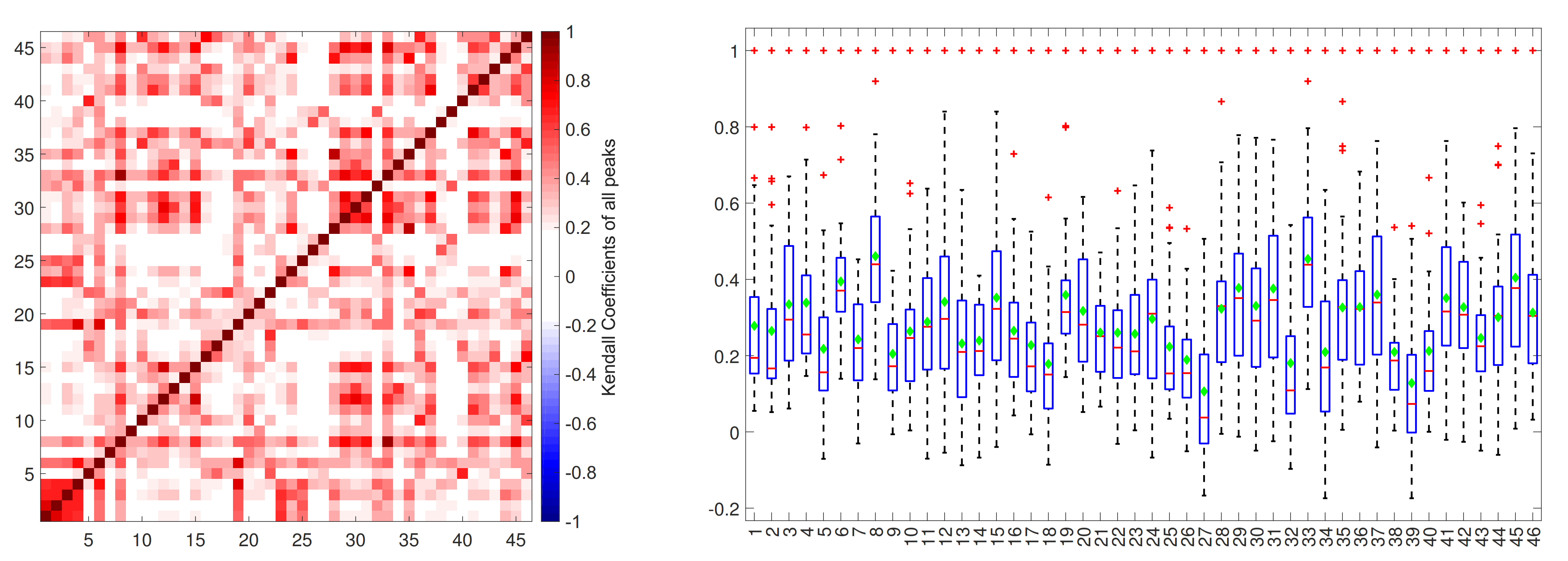
Subsequently, the Kendall tau correlation was calculated between a couple of event sets. Discharge increments also were considered in order to distinguish between the generation mechanisms and the corresponding peaks. After that, every two sites had an absolute correlation between the greatest contemporary cases. Figure 4 showed the relationship between each station to the others.
The square rank correlation matrix was plotted on the left, which is shown a positive correlation among almost all stations. The dark red shows a stronger relationship between two points, and pixels with near-zero values express no correlation. On the right figure, the range of changes in correlation was drawn. The large size catchments have a higher correlation with other catchments, and smaller catchments generally have a lower correlation. This figure showed that some of the subcatchments react opposite each other.
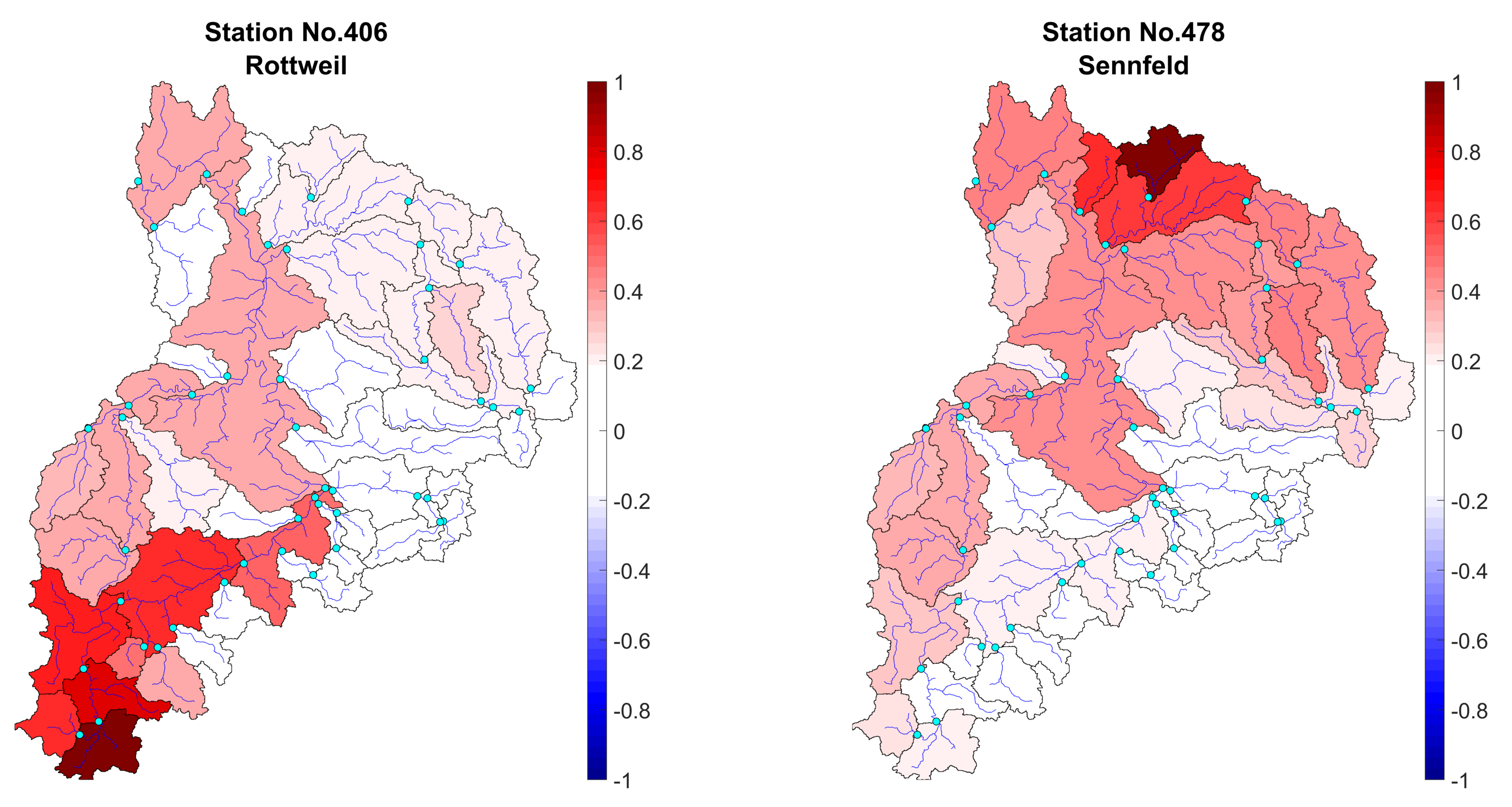
To convert this nontangible plot to an explicit configuration, Figure 5 is shown. Then, for each measurement gauge as a reference, the rank correlation was traced in the space.
Two subcatchments were selected from two distinct parts of the region to show various spatial reactions. On the left figure, Rottweil as an upstream part was settled on; the darker red shows a strong association with the reference. It shows, nearing subcatchments react at the same time and with the same harmony in this part. Also, station Sennfeld in the north had different relationships to another catchment. All red color areas had a meaningful correlation with the reference catchments in terms of vis-a-vis incidences. The proportionality of the number of catchments we have this kind of figure. Therefore, still, the behavior of the region is almost obscure. The cluster analysis, by combining 46 dimensions, provides reasonable classes in the Neckar basin.
4.2. Cluster Analyzing
4.2.1. Hierarchical Tree and Verification
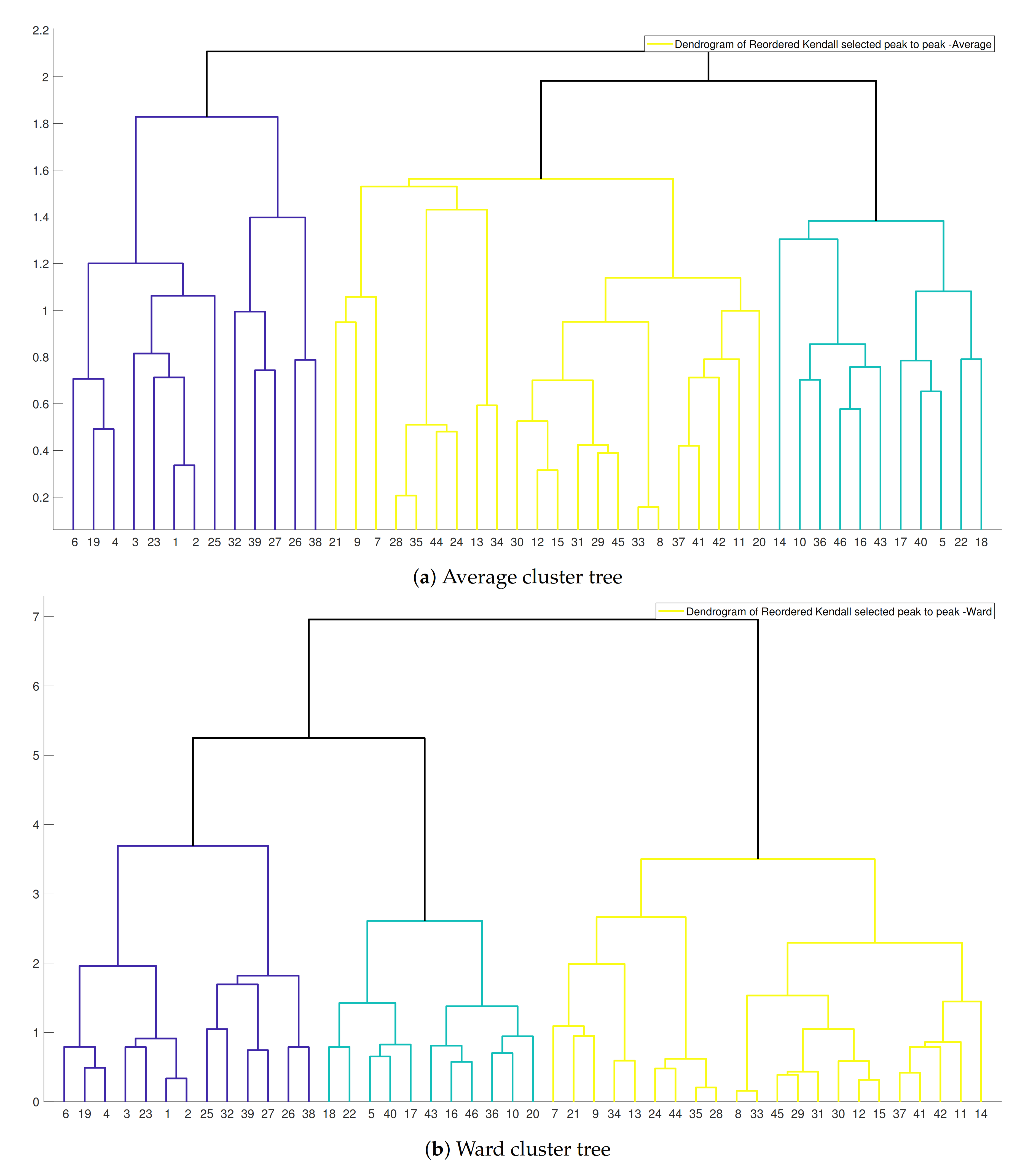
Based on computed distance matrices, hierarchical cluster trees were calculated. This clustering reflects the simultaneous behavior of extremes in different catchments. In Figure 6, two samples of the linkage method were plotted with the highest Silhouette and cophenetic indices. The shape, structure and height of trees showed distinguished companies and groups.
Dendrogram presented similarities between the contemporary peak discharge of the sampling sites. Furthermore, three main clusters in this figure are entirely vivid. However, inside each batch, there are some sub-clusters that illustrated the interconnection of sub-basins in a specific area. To decide which linkage method or corresponding tree is more relevant to this research, and as a result, do the clustering based on that, three verification methods were exerted. The mean of the inconsistency coefficient was inscribed in Table 1.
The nethermost ratio is the Single one, and all the other factors were just about the same. Due to the low number of zeros in the Single way, it might be critical to decide which linkage method is rational in this research easily. The zero coefficients express the links which had no further links below them in the hierarchical tree. This factor is independent of the distance matrix; ergo, the Cophenetic technique was applied in the pursuing step. Also, the cophenetic coefficient was calculated and written in Table 2 for five linkage algorithms.
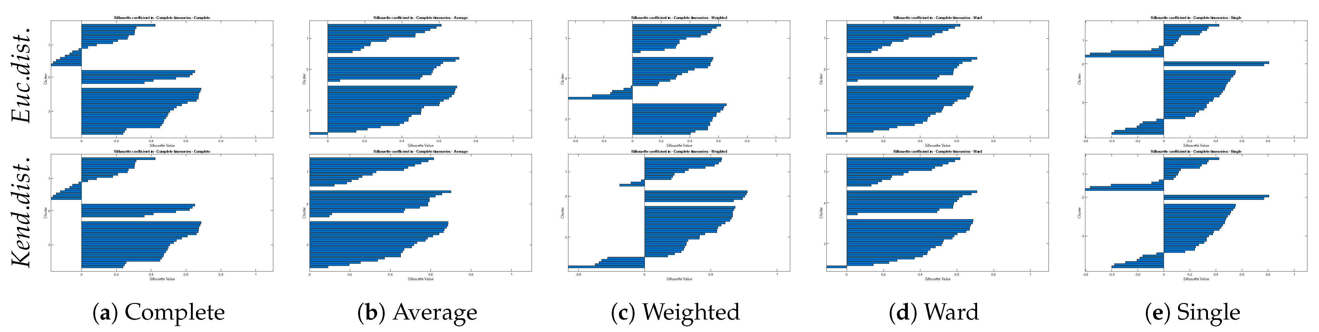
For the Euclidean distance, the Average algorithm achieved the best score and then Ward, Complete, Weighted, and Single, respectively. However, in the Kendall distance, the Average was still in the top two, but Weighted had the highest coefficient. The Single was in the third rank, and Complete and Ward were in order. So far, the Average method and then Ward or Weighted were reasonable for continuing phases of this research. However, the Single algorithm’s interpretation is for the shortest distance among the objects, and the shortest distance among dissimilarities means finding the most irrelevant catchments. Therefore, selecting the best two linkage methods took all three validation parameters into account. The Silhouette coefficients of distinct hierarchical clusters were plotted in Figure 7.
The Silhouette coefficient showed the validity of each cluster. According to Figure 7, The Complete, Weighted, and Single methods represented a lot of negative values that showed an unreliable cluster tree. Therefore, the two best possible linkage methods to cluster the simultaneously flood occurrences by employing Kendall and Euclidean distance matrix were chosen. The Kendall based distance with Average (UPGMA) linkage has no negative value in the y axis and mean coefficient of 0.4, which is the best clustering performance in this research. Also Ward linkage algorithm has almost equal to the Average method, while due to one negative value, one satiation was wrongly clustered in this method.
4.2.2. Mapping Clusters
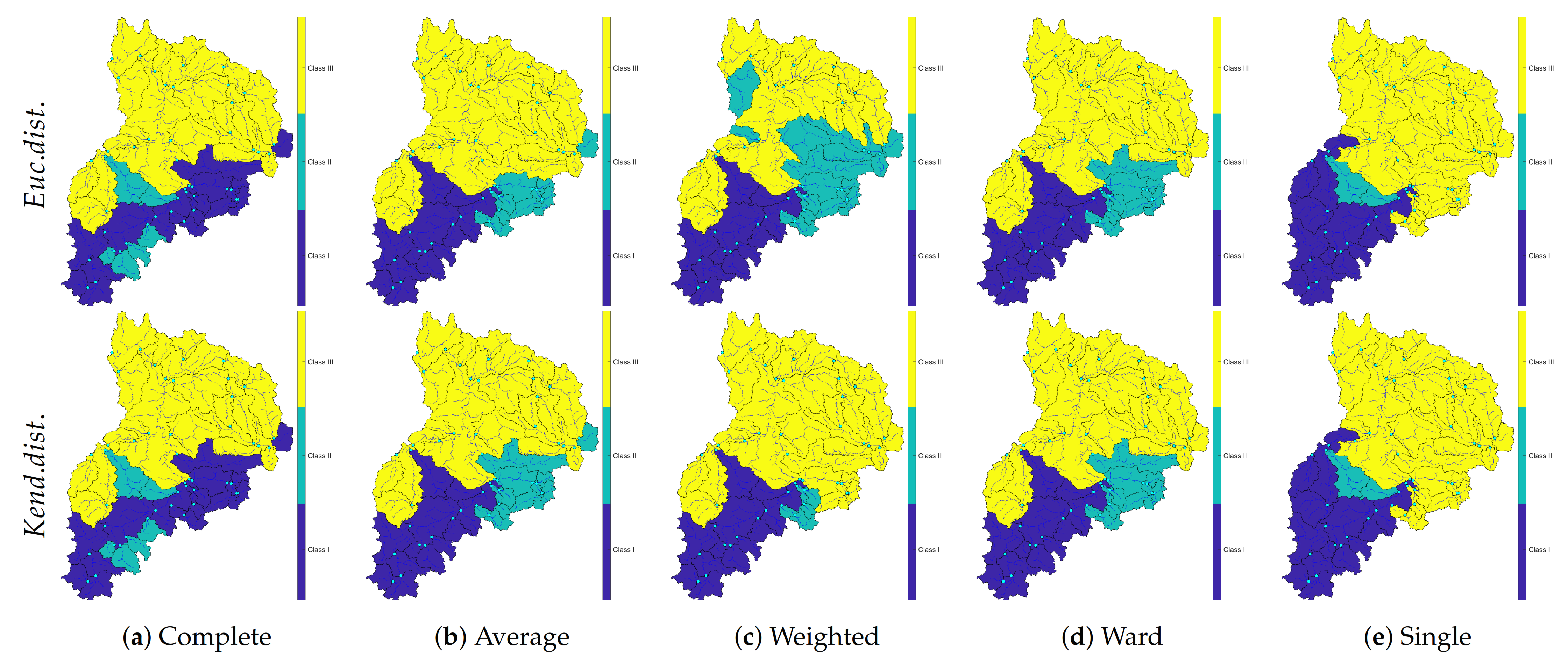
Regardless of the verification coefficients’ results, the clusters were mapped into Figure 8. These maps illustrated massive differences by employing different nexus as well as distinct distance methods.
In Figure 8 is obvious that the application of each linkage manner can make a diverse pattern. However, concerning the research objectives and the result verification on dissimilarity and inconsistency and Silhouette value, the most considerable ways to interpret clustering were selected.
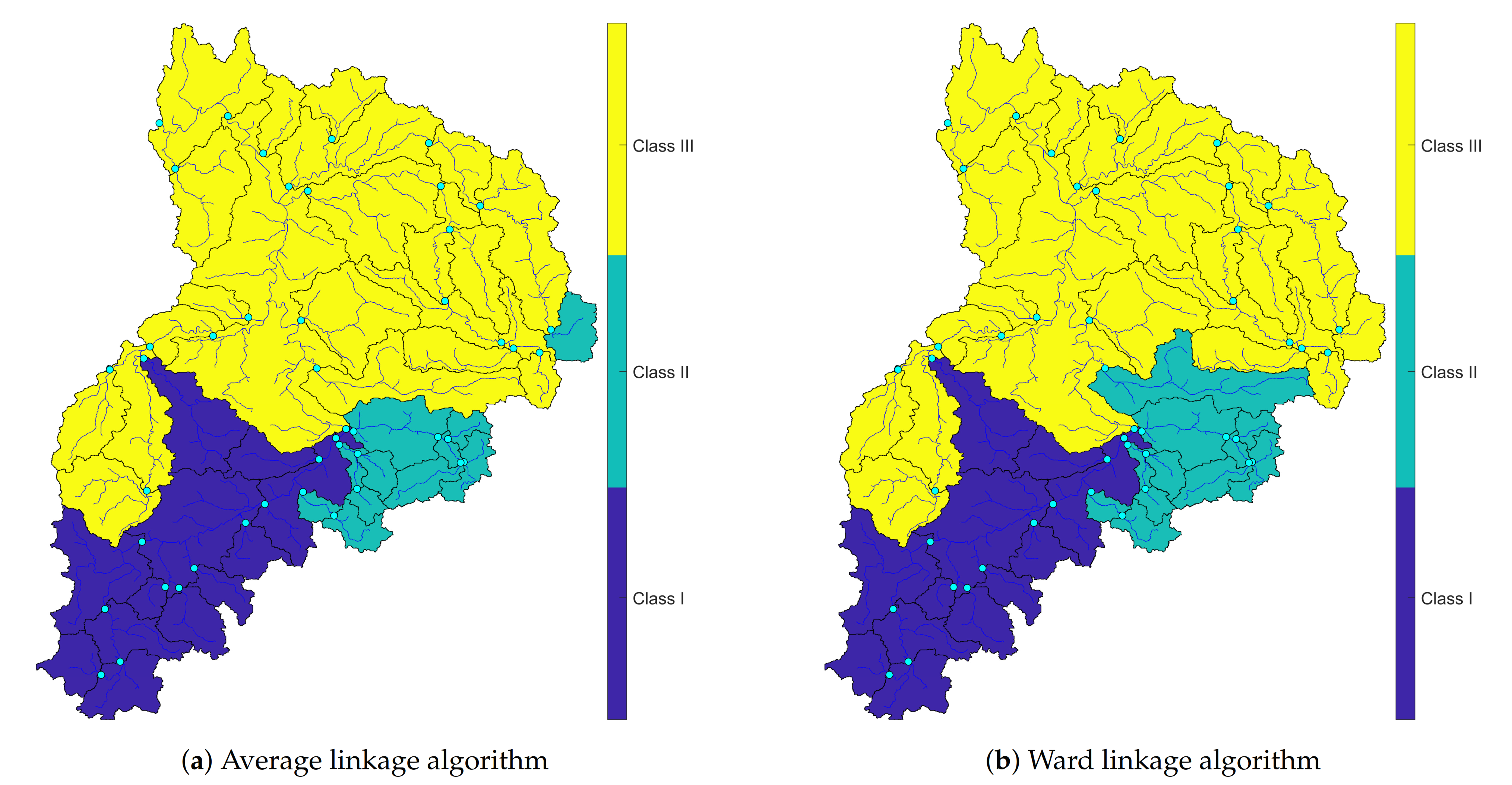
After realizing the best possible solidarity algorithm, the next step was to transform achieved outcomes and clusters to the map in a spatial domain using computed trees. In Figure 9, clustering was accomplished using Euclidean distance and with two best linkage methods. Average and Ward linkage had the best verification factors among the others.
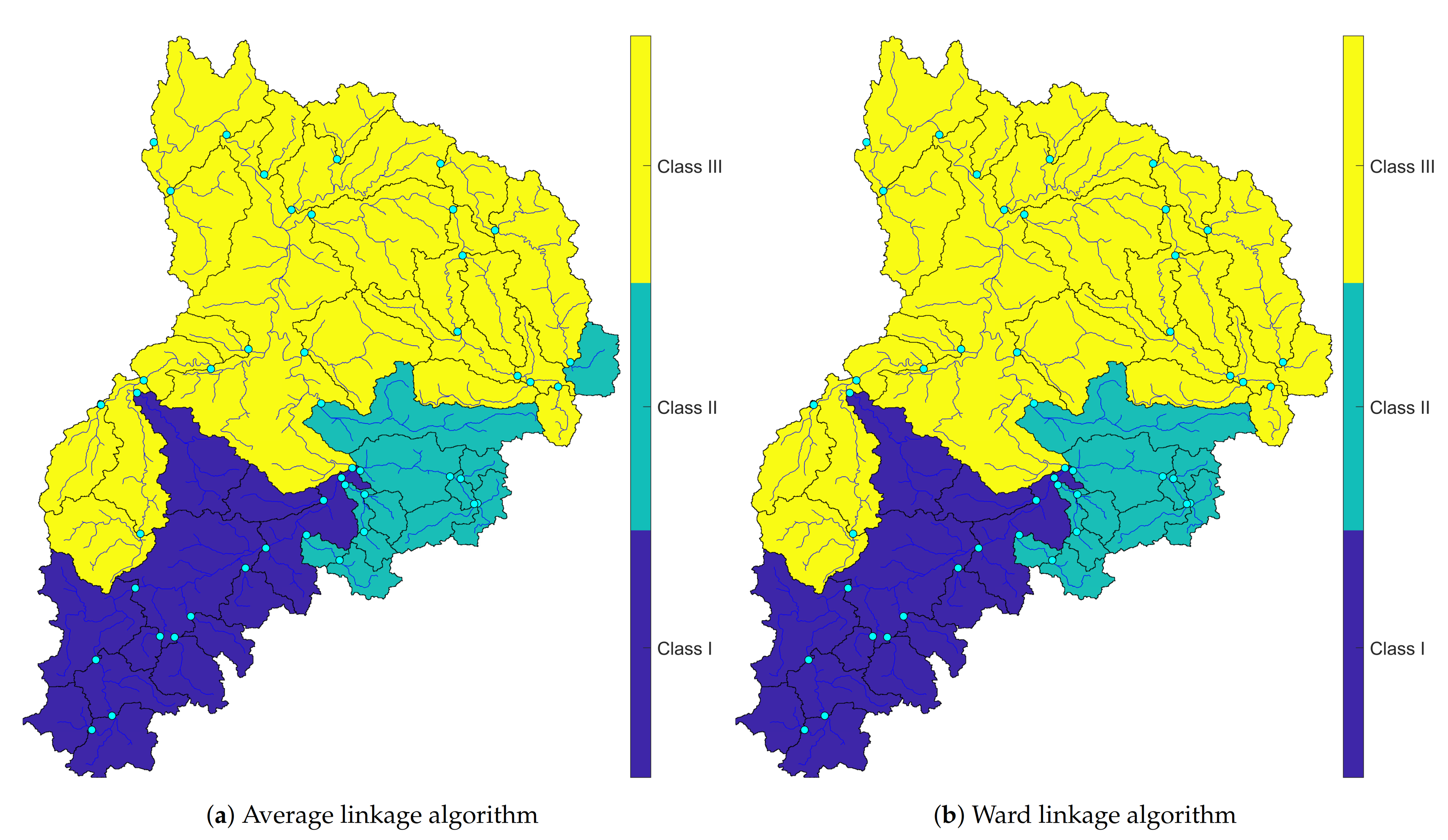
Results came from clustering represented three main regions that have a well-defined flood mechanism. In Figure 9, synchronic occurrences of flood events were clustered using Euclidean distance. In this figure, the west part of the upper Neckar catchment was wholly separated from the other sub-catchments. The Average algorithm was used in Figure 10a, and the Ward linkage method was implemented in Figure 10b. The difference between these two plots is within clusters two and three. However, they had the most common reaction areas. Afterward, the distance method was changed to discover the difference between a varied distance manner to investigate the probable difference between these two methods (see Figure 10).
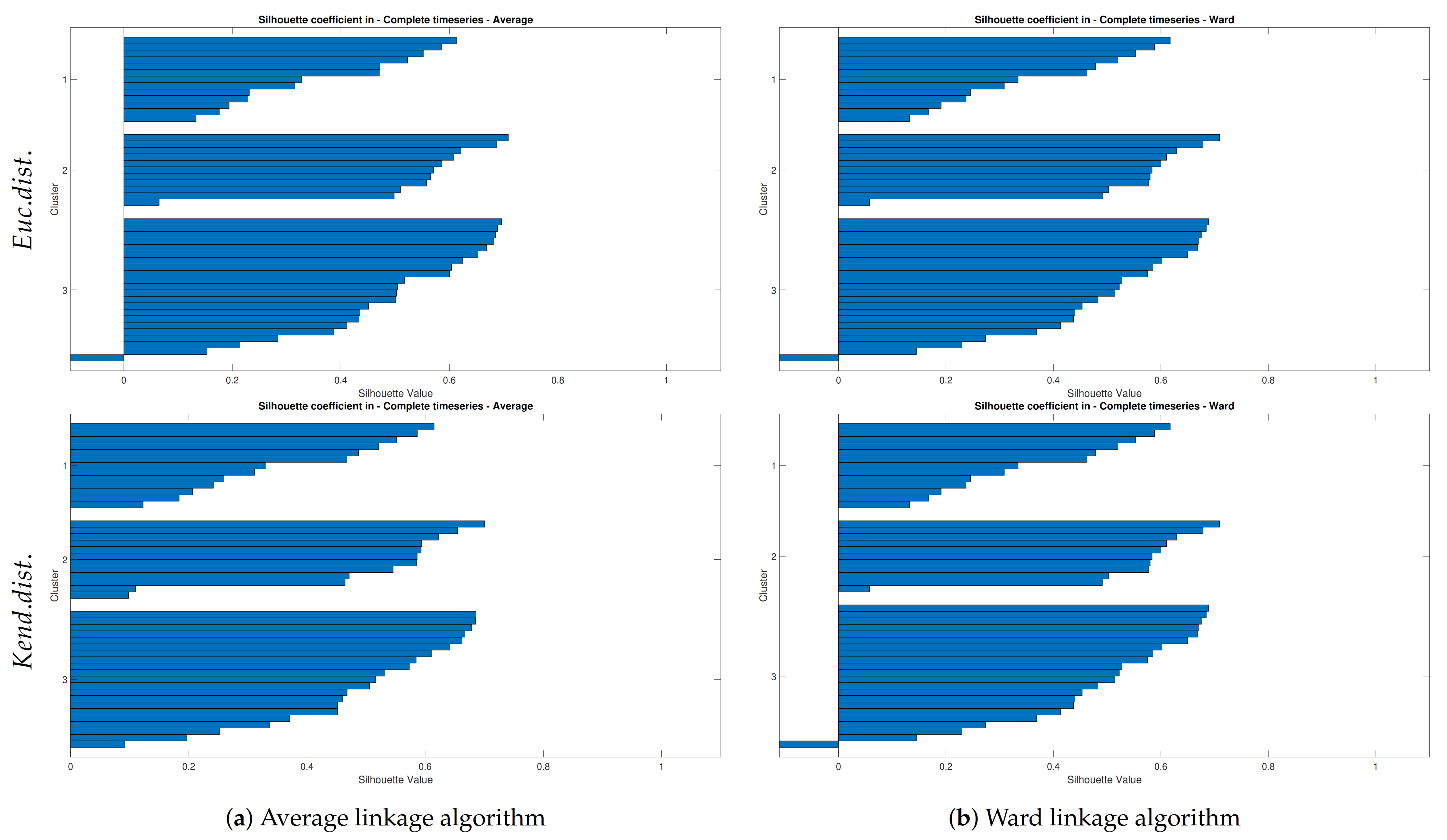
These two maps have the main pattern in clusters and only small differences between second and third clusters, which is showed in the next Figure 10. Despite changing the distance algorithm, the clustered regions were mostly identical by using these two linkage methods. Only discharge gauges Nr. 1470 and 1411 were reacted critically with this kind of clustering. To show the mentioned difference more visible, the Silhouette diagram only for Average and Ward algorithms in two distance directions was projected. Then, in continue, by doing multidimensional scaling, the final clusters have become transparent. These algorithms in two distinct distance manner were plotted to show the verification of hierarchical clustering in the Neckar basin (see Figure 11).
By plotting Silhouette coefficient diagrams of the most sensible linkage methods in Figure 11, three out of four subfigures except lower left diagram (Figure 11a) showed that a unique problem in the third cluster, which was appeared in the last figure. Therefore, despite the verification of hierarchical cluster trees in the Neckar basin, two critical stations were still dubious. Whereas the exact failed connection was detected. However, the Average linkage method employing Kendall distance plausible clustered the area.
4.3. MDS and AHCT Comparison
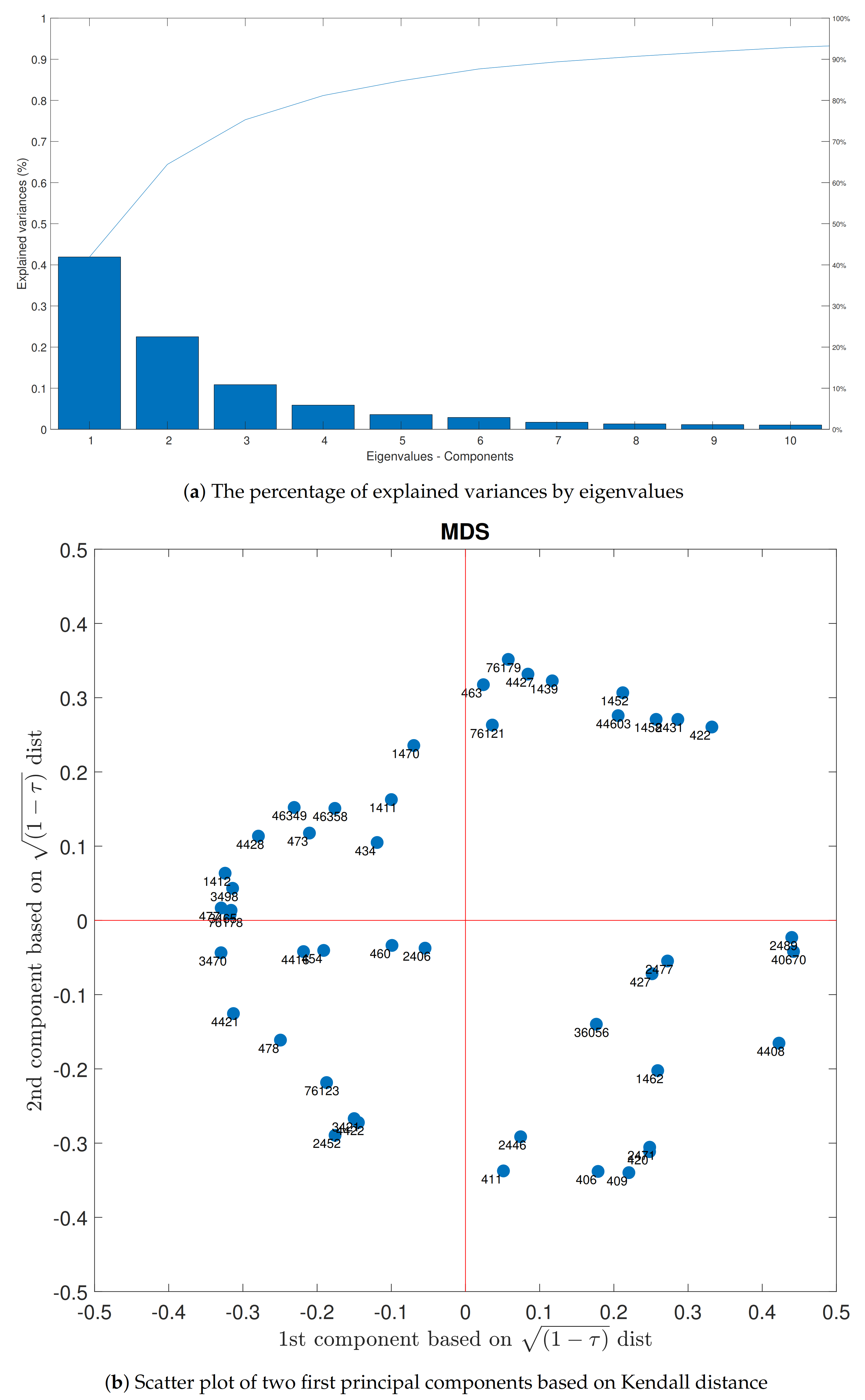
To visualize the multivariate data to the 2d plot, MDS was accomplished, and the result was revealed in Figure 12. Ten first eigenvalues plotted in Figure 12a. These components explained more than 90 percent of the total variances of the dataset. In the next part of the plot, all the stations based on the Kendall distance of the correlation matrix were converted into this map. The nearer stations had a strong relationship with each other, and farther had preferable behavior. As it came to perceive, in this plot, separated groups were apparent.
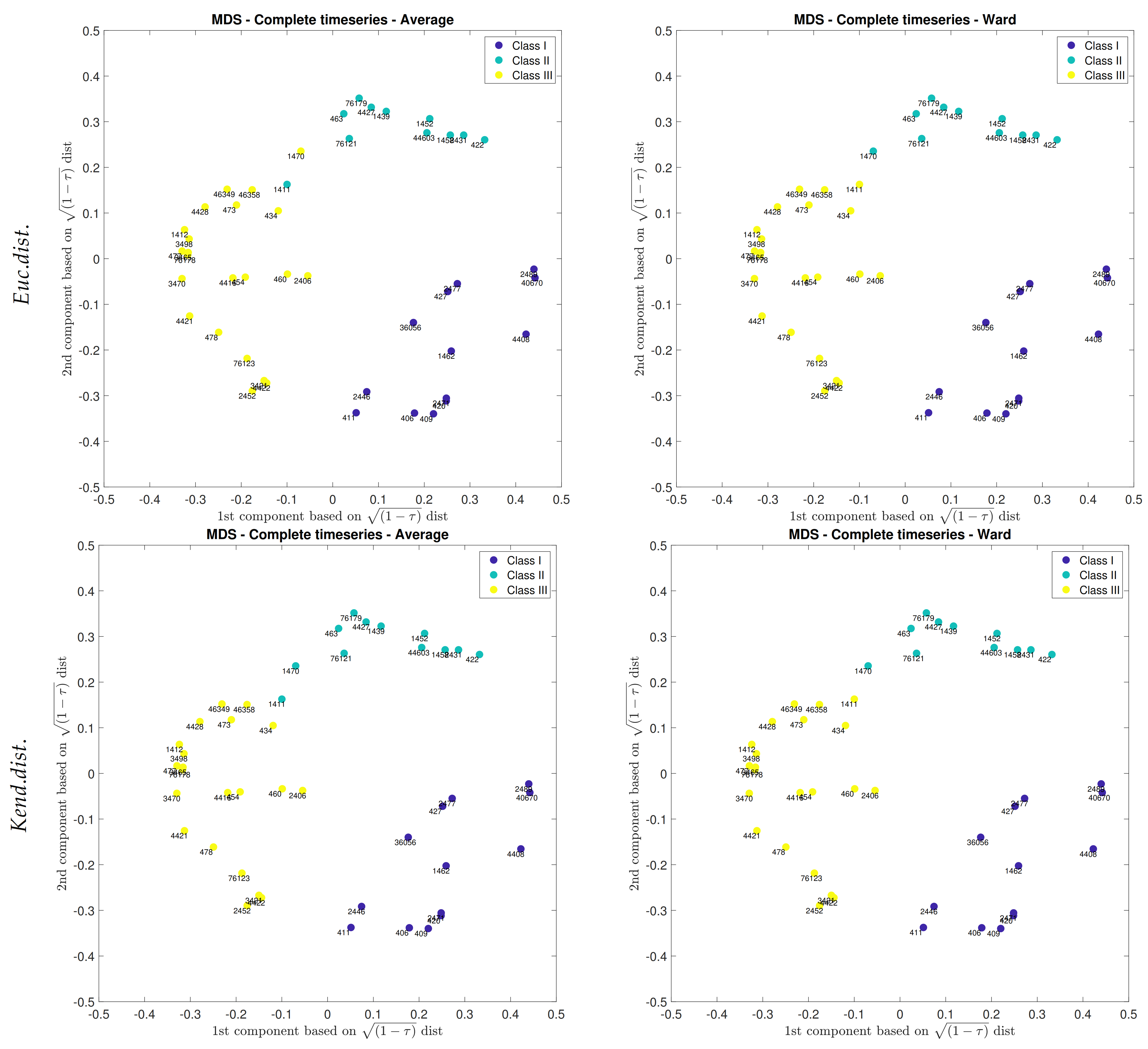
The first two components of the matrix of selected peaks were restated themselves more than 65% of the variance. By applying multidimensional scaling, interactions of the gauges were disclosed. As is lucid from Figure 12b, the map might be divided into three concentration points. Firstly is on the low right corner, secondly on the top right and one or two dots near them (Nr. 1470 or Nr. 1411) and thirdly the remaining spots. Consequently, MDS and hierarchical tree clustering with the selected linkage methods were compared on the same map (see Figure 13).
To compare the resulted cllusters in AHCT method and MDS scatter plot, three determined AHCT clusteres were transformed into two-dimensional space. Each group was drawn with a specific color that is recognizable and comparable with the others. Regarding the above Figure 13, Ward linkage worked very well with both distance matrices and showed well-defined clusters. This algorithm illustrated consistent results which were not altered by changing the way of calculation dissimilarity matrix. In the first row of the above figure, this comparison was plotted by employing Euclidean distance, and the second row is belonged to Kendall based distance. The determined and verified AHCT clusters were agreed with multidimensional scaling in a way that the near points are in a cluster and in contrast the far points are in another group. Therefore, multidimensional scaling was matched perfectly with the hierarchical clustering in both distance matrices. The small differences within the appointed nexus manner have appeared here on the upper left side of Figure 13 in utilizing euclidean distance and the Average linkage method, between the light blue and yellow clusters and exactly for the measurement gauges of 1411 and 1470 on the southeast of the basin, where the geological structure are different.
Our result support the findings and suggestion of temporal clustering of flood study in Germany that in flood clustering more than one method has to be analyzed [28], due to the nature of each clustering method. Using the AHCT method alone does not provide fixed clusters in a catchment. To have robust clusters, another complementary clustering method is required. Despite the reported statement that the spatial patterns of flood clustering behavior are not strongly pronounced in Germany [28], our clustering results show explicit cluster behaviors in concurrent occurrences of floods in the Neckar basin in Germany. The clustering result maps partly agree with the flood clustering pattern in Germany corresponds to a time windows from 1961–1990 [34]; however, our analysis is in more detail and measurement gauges.
Also, in terms of methodological approach, so far, the different hierarchical clustering algorithms are investigated, including Weighted, Average, Wards, Single, and Complete linkage methods [52,72,73,74,75,76,77], but there is not any clear suggestion that which linkage method is an appropriate algorithm in flood analysis. We found that the Ward and Average methods work very well in hydrology and flood investigation, which is in agreement with the clustering of concurrent flood risks via Hazard Scenarios research in terms of using the Average linkage method [38].
The result of this study shows an agreement with Li et al. [78] that the Silhouette factor is the integrated verification way of the cluster tree in flood investigation, owing to employ possible related variables, including similarity metrics, estimated classes, distance matrix, and tree.
5. Conclusions
The clustering of simultaneous flood occurrences in the Neckar was presented based on two independent peaks per year derived from the daily discharge time series of 46 subcatchment gauges for the time window of 1961–2015. Two multisite clustering methods were applied based on two dissimilarity indicators of Euclidean and non-parametric Kendall tau distance matrices. The AHCT clustering method also was employed five different linkage algorithms to struct the hierarchical trees. The computed trees were verified and analyzed with the Silhouette coefficient to determine the best clustering result. In total, 10 clustered zones were plotted as the result of the AHCT method and these maps were compared with the two maps of the MDS clustering method. We explored that the Neckar divided into three major regions in terms of coincident floods and the two selected clusters of MDS and AHCT are mainly agreed with each other. The first cluster is around the western part of the upper Neckar catchment and seized with the Black Forest and Swabian Alps. The second cluster is primarily located in the eastern region of the upper Neckar, with smaller subcatchment and karstic geology features. Finally, the third part is the Neckar basin’s remaining area, which is a lowland area compared to the other parts. The resulted clusters may provide four benefits for hydrologists, planners and policymakers. The first one is providing a useful indication for determining similar behavior in different measurement stations. The second one is representing a unique tool for ungauged basins evaluations in a given homogeneous zone. The third one is the early warning systems can then be upgraded by regionalizing extreme flood behavior to notify a disaster. The last one is the possibility of improvement in extreme design estimation in a cluster. Our analyses suggest some points in terms of hydrological processes and methodological approaches:
- The agglomerative hierarchical clustering and multidimensional scaling methods do not need initial assumptions, and they act independently of additional presumptions. The trees were computed based on rank correlation matrices of the highest occurrence of the floods. Both methods are recommended to apply in other case studies.
- The results show that the Average and Ward linkage methods are well-matched and verified in the Neckar basin and the Silhouette coefficient is more robust than other applied verification methods.
- Both Euclidean and Kendall tau distances act mostly the same except in the Average and weighted linkage. Therefore, AHCT is not very sensitive by changing its input distance matrix.
- The results of MDS and AHCT using Ward linkage are perfectly matched each other, which show a constant simultaneous flood occurrence pattern in the Neckar. Thus, we suggest applying the MDS method to have an initial preview of possible clusters to deliver a faster and more robust clustering process.
- The two applied methods result in similar patterns of concurrent flood clustering behavior. Therefore, we propose to employ more than one multivariate clustering method in simultaneous flood analysis to compare the obtained clusters with each other and evaluate their connection with catchment characteristics.
- The results show the simultaneous occurrences of high discharges operating as a function of the topography of the basin and seasonality of the precipitation as the primary input of hydrological analysis. It can be mentioned that a reason for some clustering mismatches might be due to the anthropogenic alterations in this area. Besides, the difference among clusters was observed in the southeast of the Neckar basin, where the geological structure is characterized by a dipping of formation, which could be the reason for the disagreements. Therefore, we suggest taking these factors into clustering consideration.
- The differences between cluster maps of AHCT and MDS have mainly occurred in small size subcatchments. To increase clustering’s robustness, merging some small upstream subcatchments as an area with a bigger size can be an appropriate option.
Our results do not support the seasonality of flood events. The seasonally based flood clustering is necessary to investigate the impact of flood generating mechanism on clustering. Also, implementing different flood identification methods may illustrate the sensitivity of applied clustering methods in analyzing simultaneous flood clustering.
Author Contributions
Conceptualization, methodology, validation, formal analysis, investigation, E.M. and A.B.; Visualization, software, writing—original draft preparation E.M.; Writing—review and editing, E.M. and A.B.; Supervision, A.B.; Project administration, E.M. and A.B.; Funding acquisition, A.B. All authors have read and agreed to the published version of the manuscript.
Funding
This research received no external funding.
Institutional Review Board Statement
Not Applicable.
Informed Consent Statement
Not Applicable.
Data Availability Statement
The discharge flow time series can be requested from the Baden-Württemberg State Institute for the Environment, Survey and Nature Conservation in (https://udo.lubw.baden-wuerttemberg.de/public/). The precipitation measurements are available on the German Weather Service’s data portal in (https://opendata.dwd.de/climate_environment/CDC/).
Acknowledgments
The authors are grateful to thank the Landesanstalt für Umwelt Baden-Württemberg (LUBW) and thank the Deutscher Wetterdienst (DWD) for providing the discharge flow and precipitation data sets. Ehsan Modiri acknowledges the Sustainable Water Management-NaWaM program from the Federal Ministry of Education and Research (BMBF) and the German Academic Exchange Service (DAAD) to support his Ph.D. Finally, we also appreciate the four anonymous reviewers’ comments and suggestions to improve this paper.
Conflicts of Interest
The authors declare no conflict of interest.
References
- Baldassarre, G.D.; Viglione, A.; Carr, G.; Kuil, L.; Salinas, J.; Blöschl, G. Socio-hydrology: Conceptualising human-flood interactions. Hydrol. Earth Syst. Sci. 2013, 17, 3295–3303. [Google Scholar] [CrossRef] [Green Version]
- European Environment Agency. Economic Losses from Climate-Related Extremes in Europe (Temporal Coverage 1980–2017); European Environment Agency: Copenhagen, Denmark, 2019. [Google Scholar]
- Schröter, K.; Kunz, M.; Elmer, F.; Mühr, B.; Merz, B. What made the June 2013 flood in Germany an exceptional event? A hydro-meteorological evaluation. Hydrol. Earth Syst. Sci. 2015, 19, 309–327. [Google Scholar] [CrossRef] [Green Version]
- van Oldenborgh, G.J.; Philip, S.; Aalbers, E.; Vautard, R.; Otto, F.; Haustein, K.; Habets, F.; Singh, R.; Cullen, H. Rapid attribution of the May/June 2016 flood-inducing precipitation in France and Germany to climate change. Hydrol. Earth Syst. Sci. Discuss. 2016, 10, 1–23. [Google Scholar]
- MunichRE. Flood/Flash Flood Events in Germany 1980–2018; Technical Report; NatCatSERVICE, Münchener Rückversicherungs-Gesellschaft “Munich RE”: Munich, Germany, 2019. [Google Scholar]
- Thieken, A.H. Floods, Flood Losses and Flood Risk Management in Germany. Ph.D. Thesis, der Universität Potsdam, Potsdam, Germany, 2009. [Google Scholar]
- Glaser, R.; Riemann, D.; Schönbein, J.; Barriendos, M.; Brázdil, R.; Bertolin, C.; Camuffo, D.; Deutsch, M.; Dobrovolnỳ, P.; van Engelen, A.; et al. The variability of European floods since AD 1500. Clim. Chang. 2010, 101, 235–256. [Google Scholar] [CrossRef]
- Hattermann, F.F.; Kundzewicz, Z.W.; Huang, S.; Vetter, T.; Kron, W.; Burghoff, O.; Merz, B.; Bronstert, A.; Krysanova, V.; Gerstengarbe, F.W. Flood Risk from a Holistic Perspective Observed Changes in Germany. In Changes in Flood Risk in Europe; Volume Special Publication No. 10; IAHS Press: Oxfordshire, UK, 2012; Chapter 11. [Google Scholar]
- Blöschl, G.; Hall, J.; Parajka, J.; Perdigão, R.A.; Merz, B.; Arheimer, B.; Aronica, G.T.; Bilibashi, A.; Bonacci, O.; Borga, M.; et al. Changing climate shifts timing of European floods. Science 2017, 357, 588–590. [Google Scholar] [CrossRef] [Green Version]
- Hall, J.; Blöschl, G. Spatial patterns and characteristics of flood seasonality in Europe. Hydrol. Earth Syst. Sci. 2018, 22, 3883–3901. [Google Scholar] [CrossRef] [Green Version]
- Blöschl, G.; Hall, J.; Viglione, A.; Perdigão, R.A.; Parajka, J.; Merz, B.; Lun, D.; Arheimer, B.; Aronica, G.T.; Bilibashi, A.; et al. Changing climate both increases and decreases European river floods. Nature 2019, 573, 1–4. [Google Scholar] [CrossRef]
- Ehmele, F.; Kunz, M. Flood-related extreme precipitation in southwestern Germany: Development of a two-dimensional stochastic precipitation model. Hydrol. Earth Syst. Sci. 2019, 23, 1083–1102. [Google Scholar] [CrossRef] [Green Version]
- Alfieri, L.; Bisselink, B.; Dottori, F.; Naumann, G.; de Roo, A.; Salamon, P.; Wyser, K.; Feyen, L. Global projections of river flood risk in a warmer world. Earth’s Future 2017, 5, 171–182. [Google Scholar] [CrossRef]
- Petrow, T.; Thieken, A.H.; Kreibich, H.; Merz, B.; Bahlburg, C.H. Improvements on flood alleviation in Germany: Lessons learned from the Elbe flood in August 2002. Environ. Manag. 2006, 38, 717–732. [Google Scholar] [CrossRef]
- Diederen, D.; Liu, Y.; Gouldby, B.; Diermanse, F.; Vorogushyn, S. Stochastic generation of spatially coherent river discharge peaks for continental event-based flood risk assessment. Nat. Hazards Earth Syst. Sci. 2019, 19, 1041–1053. [Google Scholar] [CrossRef] [Green Version]
- de Moel, H.; van Alphen, J.; Aerts, J. Flood maps in Europe–Methods, availability and use. Nat. Hazards Earth Syst. Sci. 2009, 9, 289–301. [Google Scholar] [CrossRef] [Green Version]
- Chowdhary, H.; Escobar, L.A.; Singh, V.P. Identification of suitable copulas for bivariate frequency analysis of flood peak and flood volume data. Hydrol. Res. 2011, 42, 193–216. [Google Scholar] [CrossRef]
- Li, J.; Lei, Y.; Tan, S.; Bell, C.D.; Engel, B.A.; Wang, Y. Nonstationary flood frequency analysis for annual flood peak and volume series in both univariate and bivariate domain. Water Resour. Manag. 2018, 32, 4239–4252. [Google Scholar] [CrossRef]
- Wang, C. A joint probability approach for coincidental flood frequency analysis at ungauged basin confluences. Nat. Hazards 2016, 82, 1727–1741. [Google Scholar] [CrossRef]
- Salvadori, G.; De Michele, C. Frequency analysis via copulas: Theoretical aspects and applications to hydrological events. Water Resour. Res. 2004, 40. [Google Scholar] [CrossRef]
- Favre, A.C.; El Adlouni, S.; Perreault, L.; Thiémonge, N.; Bobée, B. Multivariate hydrological frequency analysis using Copulas. Water Resour. Res. 2004, 40. [Google Scholar] [CrossRef] [Green Version]
- Heffernan, J.E.; Tawn, J.A. A conditional approach for multivariate extreme values (with discussion). J. R. Stat. Soc. Ser. (Stat. Methodol.) 2004, 66, 497–546. [Google Scholar] [CrossRef]
- Salvadori, G.; De Michele, C. Multivariate multiparameter extreme value models and return periods: A copula approach. Water Resour. Res. 2010, 46. [Google Scholar] [CrossRef]
- Salvadori, G.; Michele, C.D.; Durante, F. On the return period and design in a multivariate framework. Hydrol. Earth Syst. Sci. 2011, 15, 3293–3305. [Google Scholar] [CrossRef] [Green Version]
- Dung, N.V.; Merz, B.; Bárdossy, A.; Apel, H. Handling uncertainty in bivariate quantile estimation—An application to flood hazard analysis in the Mekong Delta. J. Hydrol. 2015, 527, 704–717. [Google Scholar] [CrossRef]
- Falter, D.; Schröter, K.; Dung, N.V.; Vorogushyn, S.; Kreibich, H.; Hundecha, Y.; Apel, H.; Merz, B. Spatially coherent flood risk assessment based on long-term continuous simulation with a coupled model chain. J. Hydrol. 2015, 524, 182–193. [Google Scholar] [CrossRef] [Green Version]
- Merz, B.; Aerts, J.; Arnbjerg-Nielsen, K.; Baldi, M.; Becker, A.; Bichet, A.; Blöschl, G.; Bouwer, L.M.; Brauer, A.; Cioffi, F.; et al. Floods and climate: Emerging perspectives for flood risk assessment and management. Nat. Hazards Earth Syst. Sci. 2014, 14, 1921–1942. [Google Scholar] [CrossRef] [Green Version]
- Merz, B.; Nguyen, V.D.; Vorogushyn, S. Temporal clustering of floods in Germany: Do flood-rich and flood-poor periods exist? J. Hydrol. 2016, 541, 824–838. [Google Scholar] [CrossRef]
- Khare, S.; Bonazzi, A.; Mitas, C.; Jewson, S. Modelling clustering of natural hazard phenomena and the effect on re/insurance loss perspectives. Nat. Hazards Earth Syst. Sci. 2015, 15, 1357–1370. [Google Scholar] [CrossRef] [Green Version]
- Villarini, G.; Smith, J.A.; Vitolo, R.; Stephenson, D.B. On the temporal clustering of US floods and its relationship to climate teleconnection patterns. Int. J. Climatol. 2013, 33, 629–640. [Google Scholar] [CrossRef]
- Vitolo, R.; Stephenson, D.B.; Cook, I.M.; Mitchell-Wallace, K. Serial clustering of intense European storms. Meteorol. Z. 2009, 18, 411–424. [Google Scholar] [CrossRef] [Green Version]
- Mailier, P.J.; Stephenson, D.B.; Ferro, C.A.T.; Hodges, K.I. Serial Clustering of Extratropical Cyclones. Mon. Weather. Rev. 2006, 134, 2224–2240. [Google Scholar] [CrossRef]
- Aubert, A.; Tavenard, R.; Emonet, R.; De Lavenne, A.; Malinowski, S.; Guyet, T.; Quiniou, R.; Odobez, J.M.; Mérot, P.; Gascuel-Odoux, C. Clustering flood events from water quality time series using Latent Dirichlet Allocation model. Water Resour. Res. 2013, 49, 8187–8199. [Google Scholar] [CrossRef]
- Beurton, S.; Thieken, A.H. Seasonality of floods in Germany. Hydrol. Sci. J. 2009, 54, 62–76. [Google Scholar] [CrossRef]
- Mediero, L.; Kjeldsen, T.; Macdonald, N.; Kohnova, S.; Merz, B.; Vorogushyn, S.; Wilson, D.; Alburquerque, T.; Blöschl, G.; Bogdanowicz, E.; et al. Identification of coherent flood regions across Europe by using the longest streamflow records. J. Hydrol. 2015, 528, 341–360. [Google Scholar] [CrossRef] [Green Version]
- Towe, R.; Tawn, J.; Eastoe, E.; Lamb, R. Modelling the clustering of extreme events for short-term risk assessment. J. Agric. Biol. Environ. Stat. 2020, 25, 32–53. [Google Scholar] [CrossRef] [Green Version]
- Wang, L.N.; Chen, X.H.; Shao, Q.X.; Li, Y. Flood indicators and their clustering features in Wujiang River, South China. Ecol. Eng. 2015, 76, 66–74. [Google Scholar] [CrossRef] [Green Version]
- Pappadà, R.; Durante, F.; Salvadori, G.; De Michele, C. Clustering of concurrent flood risks via Hazard Scenarios. Spat. Stat. 2018, 23, 124–142. [Google Scholar] [CrossRef]
- Sahu, N.; Behera, S.K.; Yamashiki, Y.; Takara, K.; Yamagata, T. IOD and ENSO impacts on the extreme stream-flows of Citarum river in Indonesia. Clim. Dyn. 2012, 39, 1673–1680. [Google Scholar] [CrossRef]
- Sahu, N.; Panda, A.; Nayak, S.; Saini, A.; Mishra, M.; Sayama, T.; Sahu, L.; Duan, W.; Avtar, R.; Behera, S. Impact of Indo-Pacific Climate Variability on High Streamflow Events in Mahanadi River Basin, India. Water 2020, 12, 1952. [Google Scholar] [CrossRef]
- LUBW. Landesanstalt für Umwelt, Messungen und Naturschutz Baden-Württemberg. Available online: https://udo.lubw.baden-wuerttemberg.de/public/ (accessed on 15 January 2021).
- DWD. Wetter und Klima–Deutscher Wetterdienst –CDC (Climate Data Center). Available online: https://opendata.dwd.de/climate_environment/CDC/ (accessed on 15 January 2021).
- Bárdossy, A.; Pegram, G. Infilling missing precipitation records—A comparison of a new Copula-based method with other techniques. J. Hydrol. 2014, 519, 1162–1170. [Google Scholar] [CrossRef]
- Emblemsvåg, J. Risk Management for the Future: Theory and Cases; IntechOpen: London, UK, 2012. [Google Scholar]
- Seidel, J.; Dostal, P.; Imbery, F. Analysis of Historical River Floods-A Contribution Towards Modern Flood Risk Management. In Risk Management for the Future-Theory and Cases; Emblemsvåg, J., Ed.; IntechOpen: London, UK, 2012; Chapter 12; pp. 275–294. [Google Scholar]
- Bürger, K.; Dostal, P.; Seidel, J.; Imbery, F.; Barriendos, M.; Mayer, H.; Glaser, R. Hydrometeorological reconstruction of the 1824 flood event in the Neckar River basin (southwest Germany). Hydrol. Sci. J. 2006, 51, 864–877. [Google Scholar] [CrossRef]
- Götzinger, J.; Barthel, R.; Jagelke, J.; Bárdossy, A. The role of groundwater recharge and baseflow in integrated models. In Proceedings of the Symposium IUGG HS1002; IAHS Publication: Perugia, Italy, 2007; Volume 321, pp. 103–109. [Google Scholar] [CrossRef]
- Jagelke, J.; Barthel, R. Conceptualization and implementation of a regional groundwater model for the Neckar catchment in the framework of an integrated regional model. Adv. Geosci. 2005, 5, 105–111. [Google Scholar] [CrossRef] [Green Version]
- Kalweit, H.; Buck, W.; Felkel, k.; Gerhard, H.; Malde, J.; Nippes, K.R.; Ploeger, B.; Schmitz, W. Der Rhein unter der Einwirkung des Menschen: Ausbau, Schiffahrt, Wasserwirtschaft; CHR/KHR: Utrecht, The Netherlands, 1993. [Google Scholar]
- Bormann, H. Runoff regime changes in German rivers due to climate change. Erdkunde 2010, 64, 257–279. [Google Scholar] [CrossRef]
- Kendall, M.G. Rank Correlation Methods.; Charles Griffin & Co. Ltd.: London, UK, 1948. [Google Scholar]
- Jain, A.K.; Murty, M.N.; Flynn, P.J. Data clustering: A review. ACM Comput. Surv. (CSUR) 1999, 31, 264–323. [Google Scholar] [CrossRef]
- Unal, Y.; Kindap, T.; Karaca, M. Redefining the climate zones of Turkey using cluster analysis. Int. J. Climatol. J. R. Meteorol. Soc. 2003, 23, 1045–1055. [Google Scholar] [CrossRef]
- Lyra, G.B.; Oliveira-Júnior, J.F.; Zeri, M. Cluster analysis applied to the spatial and temporal variability of monthly rainfall in Alagoas state, Northeast of Brazil. Int. J. Climatol. 2014, 34, 3546–3558. [Google Scholar] [CrossRef]
- Corporal-Lodangco, I.L.; Leslie, L.M. Defining Philippine Climate Zones Using Surface and High-Resolution Satellite Data. Procedia Comput. Sci. 2017, 114, 324–332. [Google Scholar] [CrossRef]
- Santos, C.A.G.; Moura, R.; da Silva, R.M.; Costa, S.G.F. Cluster Analysis Applied to Spatiotemporal Variability of Monthly Precipitation over Paraíba State Using Tropical Rainfall Measuring Mission (TRMM) Data. Remote Sens. 2019, 11, 637. [Google Scholar] [CrossRef] [Green Version]
- Kaufman, L.; Rousseeuw, P.J. Finding Groups in Data: An Introduction to Cluster Analysis; John Wiley & Sons: Hoboken, NJ, USA, 2009; Volume 344. [Google Scholar]
- Davidson, I.; Ravi, S.S. Agglomerative Hierarchical Clustering with Constraints: Theoretical and Empirical Results; Knowledge Discovery in Databases: PKDD 2005; Jorge, A.M., Torgo, L., Brazdil, P., Camacho, R., Gama, J., Eds.; Springer: Berlin/Heidelberg, Germany, 2005; pp. 59–70. [Google Scholar]
- Ward, J.H., Jr. Hierarchical grouping to optimize an objective function. J. Am. Stat. Assoc. 1963, 58, 236–244. [Google Scholar] [CrossRef]
- Murtagh, F.; Legendre, P. Ward’s Hierarchical Agglomerative Clustering Method: Which Algorithms Implement Ward’s Criterion? J. Classif. 2014, 31, 274–295. [Google Scholar] [CrossRef] [Green Version]
- Bar-Joseph, Z.; Gifford, D.K.; Jaakkola, T.S. Fast optimal leaf ordering for hierarchical clustering. Bioinformatics 2001, 17, S22–S29. [Google Scholar] [CrossRef] [PubMed] [Green Version]
- Zahn, C.T. Graph-theoretical methods for detecting and describing gestalt clusters. IEEE Trans. Comput. 1971, 100, 68–86. [Google Scholar] [CrossRef] [Green Version]
- Jain, A.K.; Dubes, R.C. Algorithms for Clustering Data; Prentice Hall: Englewood Cliffs, NY, USA, 1988. [Google Scholar]
- Sokal, R.R.; Rohlf, F.J. The comparison of dendrograms by objective methods. Taxon 1962, 11, 33–40. [Google Scholar] [CrossRef]
- Farris, J.S. On the cophenetic correlation coefficient. Syst. Zool. 1969, 18, 279–285. [Google Scholar] [CrossRef] [Green Version]
- Holgersson, M. The limited value of cophenetic correlation as a clustering criterion. Pattern Recognit. 1978, 10, 287–295. [Google Scholar] [CrossRef]
- Rousseeuw, P.J. Silhouettes: A graphical aid to the interpretation and validation of cluster analysis. J. Comput. Appl. Math. 1987, 20, 53–65. [Google Scholar] [CrossRef] [Green Version]
- Kruskal, J.B.; Wish, M. Multidimensional Scaling (Quantitative Applications in the Social Sciences); Sage Publications, Inc.: Beverly Hills, CA, USA, 1978. [Google Scholar]
- Torgerson, W.S. Multidimensional scaling: I. Theory and method. Psychometrika 1952, 17, 401–419. [Google Scholar] [CrossRef]
- Seber, G. Multivariate Observations; John Wiley & Sons: New York, NY, USA, 1984. [Google Scholar]
- Hintze, J. Multidimensional Scaling, Help Documentation, Chapter 435. NCSS 2019 Statistical Software; NCSS, LLC.: Kaysville, UT, USA, 2019. [Google Scholar]
- Bouguettaya, A. On-line clustering. IEEE Trans. Knowl. Data Eng. 1996, 8, 333–339. [Google Scholar] [CrossRef]
- Bouguettaya, A.; Yu, Q.; Liu, X.; Zhou, X.; Song, A. Efficient agglomerative hierarchical clustering. Expert Syst. Appl. 2015, 42, 2785–2797. [Google Scholar] [CrossRef]
- Day, W.H.E.; Edelsbrunner, H. Efficient algorithms for agglomerative hierarchical clustering methods. J. Classif. 1984, 1, 7–24. [Google Scholar] [CrossRef]
- Murtagh, F.; Contreras, P. Methods of Hierarchical Clustering. arXiv 2011, arXiv:1105.0121. [Google Scholar]
- Murtagh, F.; Contreras, P. Algorithms for hierarchical clustering: An overview. Wiley Interdiscip. Rev. Data Min. Knowl. Discov. 2012, 2, 86–97. [Google Scholar] [CrossRef]
- Senthilnath, J.; Rajendra, R.; Suresh, S.; Kulkarni, S.; Benediktsson, J. Hierarchical clustering approaches for flood assessment using multi-sensor satellite images. Int. J. Image Data Fusion 2019, 10, 28–44. [Google Scholar] [CrossRef]
- Li, J.; Hassan, D.; Brewer, S.; Sitzenfrei, R. Is Clustering Time-Series Water Depth Useful? An Exploratory Study for Flooding Detection in Urban Drainage Systems. Water 2020, 12, 2433. [Google Scholar] [CrossRef]
Figure 1.
Location of the Neckar catchment in the southwest of Germany; yellow: Germany, cyan: the state of Baden-Württemberg, red: the Neckar catchment and its 46 subcatchments.
Figure 1.
Location of the Neckar catchment in the southwest of Germany; yellow: Germany, cyan: the state of Baden-Württemberg, red: the Neckar catchment and its 46 subcatchments.

Figure 2.
The procedure of flood events identification in discharge time series (m3/s); red dots: independent peaks, red circles: individual events, yellow stars: correspond peak in other time series, yellow lines: the bound of selecting correspond peaks.
Figure 2.
The procedure of flood events identification in discharge time series (m3/s); red dots: independent peaks, red circles: individual events, yellow stars: correspond peak in other time series, yellow lines: the bound of selecting correspond peaks.

Figure 3.
The flow diagram of clustering simultaneous occurrence of extreme flood events.

Figure 4.
Kendall rank correlation among all pair set of extremes; In the box plot, red plus: outliers, central red line: median, green diamond: mean.
Figure 4.
Kendall rank correlation among all pair set of extremes; In the box plot, red plus: outliers, central red line: median, green diamond: mean.

Figure 5.
The simultaneous occurrence of the most significant floods regarding the reference stations; (Left) Rottweil; (Right) Sennfeld.
Figure 5.
The simultaneous occurrence of the most significant floods regarding the reference stations; (Left) Rottweil; (Right) Sennfeld.

Figure 6.
Hierarchical cluster tree of the simultaneous occurrence of the biggest floods.

Figure 7.
Silhouette coefficient of different hierarchical trees.

Figure 8.
Spatial mapping of different hierarchical clustering.

Figure 9.
Clustering the simultaneous occurrences of the biggest flood events using Euclidean dist.

Figure 10.
Clustering the simultaneous occurrences of the biggest flood events using Kendall dist.

Figure 11.
Silhouette coefficient of different hierarchical clusters.

Figure 12.
Multidimensional scaling of the biggest floods in the Neckar catchment.

Figure 13.
Comparison between multidimensional scaling and hierarchical clusters.


Table 1.
Mean of inconsistency coefficient of the hierarchical cluster tree.
| Dist. | Complete | Average | Weighted | Ward | Single | |
|---|---|---|---|---|---|---|
| Inconsistency coefficient | Euc. dist. | 0.542 | 0.540 | 0.542 | 0.544 | 0.515 |
| Kend. dist. | 0.524 | 0.543 | 0.561 | 0.537 | 0.513 | |
| Number of zeros | Euc. dist. | 17 | 16 | 16 | 18 | 15 |
| Kend. dist. | 18 | 15 | 15 | 18 | 14 |
Table 2.
The cophenetic coefficient of various linkage methods based on distance matrices.
| Complete | Average | Weighted | Ward | Single | |
|---|---|---|---|---|---|
| Euclidean distance | 0.725 | 0.787 | 0.676 | 0.730 | 0.630 |
| Kendall distance | 0.672 | 0.784 | 0.786 | 0.649 | 0.710 |
Publisher’s Note: MDPI stays neutral with regard to jurisdictional claims in published maps and institutional affiliations. |
© 2021 by the authors. Licensee MDPI, Basel, Switzerland. This article is an open access article distributed under the terms and conditions of the Creative Commons Attribution (CC BY) license (http://creativecommons.org/licenses/by/4.0/).
Share and Cite
MDPI and ACS Style
Modiri, E.; Bárdossy, A. Clustering Simultaneous Occurrences of the Extreme Floods in the Neckar Catchment. Water 2021, 13, 399. https://doi.org/10.3390/w13040399
AMA Style
Modiri E, Bárdossy A. Clustering Simultaneous Occurrences of the Extreme Floods in the Neckar Catchment. Water. 2021; 13(4):399. https://doi.org/10.3390/w13040399
Chicago/Turabian StyleModiri, Ehsan, and András Bárdossy. 2021. "Clustering Simultaneous Occurrences of the Extreme Floods in the Neckar Catchment" Water 13, no. 4: 399. https://doi.org/10.3390/w13040399
Note that from the first issue of 2016, this journal uses article numbers instead of page numbers. See further details here.