
A Stochastic Procedure for Temporal Disaggregation of Daily Rainfall Data in SuDS Design
by
 , , and
Matteo Pampaloni
1,2,*, 
Alvaro Sordo-Ward
2,
Paola Bianucci
2,
Ivan Gabriel-Martin
2,
Enrica Caporali
1 and
Luis Garrote
2 1
Department of Civil and Environmental Engineering, University of Florence, 50139 Florence, Italy
2
Departamento de Ingeniería Civil, Hidráulica, Energía y Medio Ambiente, Universidad Politécnica de Madrid (UPM), 28040 Madrid, Spain
*
Author to whom correspondence should be addressed.
Water 2021, 13(4), 403; https://doi.org/10.3390/w13040403
Submission received: 9 December 2020
/
Revised: 22 January 2021
/
Accepted: 30 January 2021
/
Published: 4 February 2021
(This article belongs to the Special Issue Planning and Management of Hydraulic Infrastructure)
Abstract
:Hydrological design of Sustainable urban Drainage Systems (SuDS) is commonly achieved by estimating rainfall volumetric percentiles from daily rainfall series. Nevertheless, urban watersheds demand rainfall data at sub-hourly time step. Temporal disaggregation of daily rainfall records using stochastic methodologies can be applied to improve SuDS design parameters. This paper is aimed to analyze the ability of the synthetic rainfall generation process to reproduce the main characteristics of the observed rainfall and the estimation of the hydrologic parameters often used for SuDS design and by using the generally available daily rainfall data. Other specifics objectives are to analyze the effect of Minimum Inter-event Time (MIT) and storm volume threshold on rainfall volumetric percentiles commonly used in SuDS design. The reliability of the stochastic spatial-temporal model RainSim V.3 to reproduce observed key characteristics of rainfall pattern and volumetric percentiles, was also investigated. Observed and simulated continuous rainfall series with sub-hourly time-step were used to calculate four key characteristics of rainfall and two types of rainfall volumetric percentiles. To separate independent rainstorm events, MIT values of 3, 6, 12, 24, 48 and 72 h and storm volume thresholds of 0.2, 0.5, 1 and 2 mm were considered. Results show that the proposed methodology improves the estimation of the key characteristics of the rainfall events as well as the hydrologic parameters for SuDS design, compared with values directly deduced from the observed rainfall series with daily time-step. Moreover, MITs rainfall volumetric percentiles of total number of rainfall events are very sensitive to MIT and threshold values, while percentiles of total volume of accumulated rainfall series are sensitive only to MIT values.
1. Introduction
Currently, more than half of the world population lives in urban areas and a growth is expected [1]. Human activity on urban basins induced changes on the hydrological characteristics, such as increased runoff volume and rates, decreased runoff lag time, reduction of aquifer recharge and severe effects on water quality [2]. Conventional stormwater management practices, like surface water networks and combined sewerage systems, may turn out to be unsustainable. They are costly and have a limited ability to treat outlet contaminants, to reduce runoff volume and peak flow and to adapt to changes, for example, the expansion of urbanized areas and increase of storm frequency due to climate change [3]. In recent years, alternative stormwater management practices, such as Sustainable urban Drainage Systems (SuDS), have been adopted to address these issues and present different characteristics that potentially make these facilities attractive to developers and local administrations [4,5]. SuDS are blue-green structures which work reinstating natural elements of urban catchment with the aim of retaining rainfall, retarding its movement through the surface network, restore infiltration and evapotranspiration through natural or seminatural processes, improve water quality, among others [6,7,8]. Water and pollutants in urban landscapes may be retained by a combination of conventional methods supported by SuDS structures, like pervious pavements, infiltration trenches, swales, filter strips, filter drains for the streetscape, soakaways, infiltration and detention basins, bioretention areas, ponds and wetlands, trees for open spaces, green roofs and attenuation tanks for special uses, among others [6,9,10,11]. From the standpoint of engineering modelling practice, hydrological and hydraulic design parameters for SuDS follow its geometrical discretization: (a) vegetation and volume fraction, surface slope, surface roughness and storage depth for surface layer; (b) thickness, permeability and impervious fraction for pavement layer if present; (c) thickness, porosity, field capacity, hydraulic conductivity and suction head for soil layer; (d) thickness and void ratio for storage layer if present; (e) flow coefficient, control volume and flow capacity for drain layer if present [12]. As highlighted by many authors, the analysis of rainfall spectrum and its consequences represents a key component of the design of urban drainage systems. Historical data collected by a rain gauge can be considered as a sequence of rainstorm events composed by very frequent, common, heavy and finally extreme ones [13,14]. Although extreme events are connected with pluvial floods of higher intensities, small and moderate rainstorm events are responsible for most of the runoff and mass pollutant discharges, representing in many cases the most important storms for SuDS characterization [15,16]. Some authors stated that urban flood management should be addressed with a holistic and long-term vision to achieve a resilient and cost-effective solution [10,17]. Fratini et al. [17] proposed the use of the 3 Point Approach (3PA), developed by Geldof and Kluck [18], as a tool for decision-making process in urban flood management. Smit Andersen et al. [13] followed the qualitative approach proposed by [17] to select the representative storms for analyzing the design and functioning of a SuDS. They showed that SuDS may not be efficient on mitigating extreme events. SuDS performed better in the field of Small Storm Hydrology of urban environments [19]. Therefore, hydrological design of SuDS is usually based on rainfall percentiles to be managed. The formulation and selection of these rainfall percentiles can be made following different criteria, as the number of rainstorm events or the accumulated volume of the rainfall series to be managed [6,20,21,22]. In small urban watersheds there are two different ways of using rainfall-runoff hydrological models. By one side, the design storm approach relates the concept of return period and various severity grades of extreme rainfall forcing can be applied to the facility under design. On the other hand, the approach consists to achieve continuous streamflow series from the numerical model using historical or synthetic rainfall records as input [23,24]. The most accurate rainfall data can be obtained from rain gauges, with typical temporal aggregation between 5 min and 1 h due to the small size of the urban catchments and short time of concentrations occurred [25]. This high-resolution type of data is required for SuDS planning and designing. However, in general, only rainfall data with daily temporal aggregation is often found all over the world [26,27]. Rainfall disaggregation produced by stochastic rainfall generators can be an attractive option to overcome this fine-scale rainfall data requirement. Different types of stochastic models exist to generate n-years series of point (or areal) rainfall at sub-hourly resolutions. First type of methods is based on Markov Chain modelling [28], that use a miscellaneous of rainfall probability distribution functions (e.g., Exponential, Gamma, Weibull, Generalized Pareto—GPD, etc.) to describe the characteristics of rainfall ranging from low to high intensities. The second type is represented by the Rectangular Pulse model, as proposed in Neyman-Scott [29] and Barlett-Lewis [30], both schematizing storms as clusters of rain cells by means of rectangular pulses. Storm occurrences are described by means of Poisson processes: cell rainfall arrivals are random in time with exponential interarrival times, which are independent from each other. A join between a Semi–Markov Chain based and the Neyman–Scott rectangular pulse stochastic generator was introduced by some authors in order to consider atmospheric indices, as in the Markov Chain models, as a condition to the model [31,32]. Nevertheless, applications of these different disaggregation stochastic methodologies to SuDS design are not fully developed [33]. Occurrence of rainstorm events can be characterized by some statistical parameters like number of rainfall events, storm durations, intensities and cumulated depths as well as inter-event times [34]. To analyze key properties of rainstorm events, separation of time series of point-rainfall records into individual and independent rainfall events is needed. Several methods are reported in the literature to identify independent rainstorm events, like autocorrelation method [35], rank correlation method [36] and exponential method [37]. Alternatively, some authors suggested that key statistical properties of rainstorms can vary significantly depending on: (a) the minimum temporal resolution time-step of rainfall series; (b) the minimum antecedent dry weather period to be used in separating independent rainstorm events; (c) storm volume threshold, that is, the minimum precipitation volume that must be exceeded to consider a storm occurrence as an event [38,39]. For SuDS design, both (b) and (c) depend on the specific facility to be designed. Despite the numerous studies related to storm characterization, the correct definition of (b) and (c) values for each type of urban drainage design are vague and arbitrary [24]. In this paper, we develop a quantitative and probabilistic method to estimate SuDS design parameters. Specifically, we propose a temporal disaggregation methodology based on the Neyman-Scott Rectangular Pulse Method, applied in a single site, by using the stochastic rainfall generator model RainSim V.3 [31]. The model application is carried out with reference to the Florence University rain gauge located in Florence (Tuscany, Italy). A 20–year long series of observed precipitation volumes, recorded every 15 min, is available and was used to define the current scenario. The main objective of this study is to analyze the ability of the proposed methodology to estimate hydrologic parameters often used for SuDS design and by using the generally available daily rainfall data. Another two specific objectives are achieved: to verify the ability of the stochastic generator to reproduce observed key properties of storm events and to analyze the dependence of SuDS design parameters with the minimum antecedent dry weather period and the storm volume threshold considered.
The paper is structured as follow. First, a description of the case study, consisting of 20-years rainfall data of the Florence University gauge station, is presented. Then, a full description of the methodology adopted is provided (Section 2). After a brief summary scheme of the entire activities and procedures, the stochastic rainfall generator RainSim V.3 (Section 2.1) is described. After that, we describe the procedure to identify independent rainstorm events using minimum antecedent dry weather period and storm volume threshold as variables of the process and we describe calculation of key characteristics of rainfall patterns (Section 2.2). Lastly, SuDS design parameters calculation are explained, describing the double approach based on percentiles of total number of rainfall events and of the total volume of accumulated rainfall series (Section 2.3). In Section 3. Results and discussion, we present the results of RainSim V.3 validation by calculating and comparing aforementioned key characteristics of rainfall patterns (Section 3.1). Second, the ability of the stochastic rainfall generator to reproduce rainfall volumetric percentiles commonly used in SuDS design (Section 3.2) is tested. Third, we conduct the sensitivity analysis of SuDS rainfall volumetric percentiles, both for observed and simulated series, using different minimum antecedent dry weather periods and storm volume thresholds as variables of the process (Section 3.3). Lastly, the main conclusions of the work (Section 4) are presented.
2. Materials and Methods
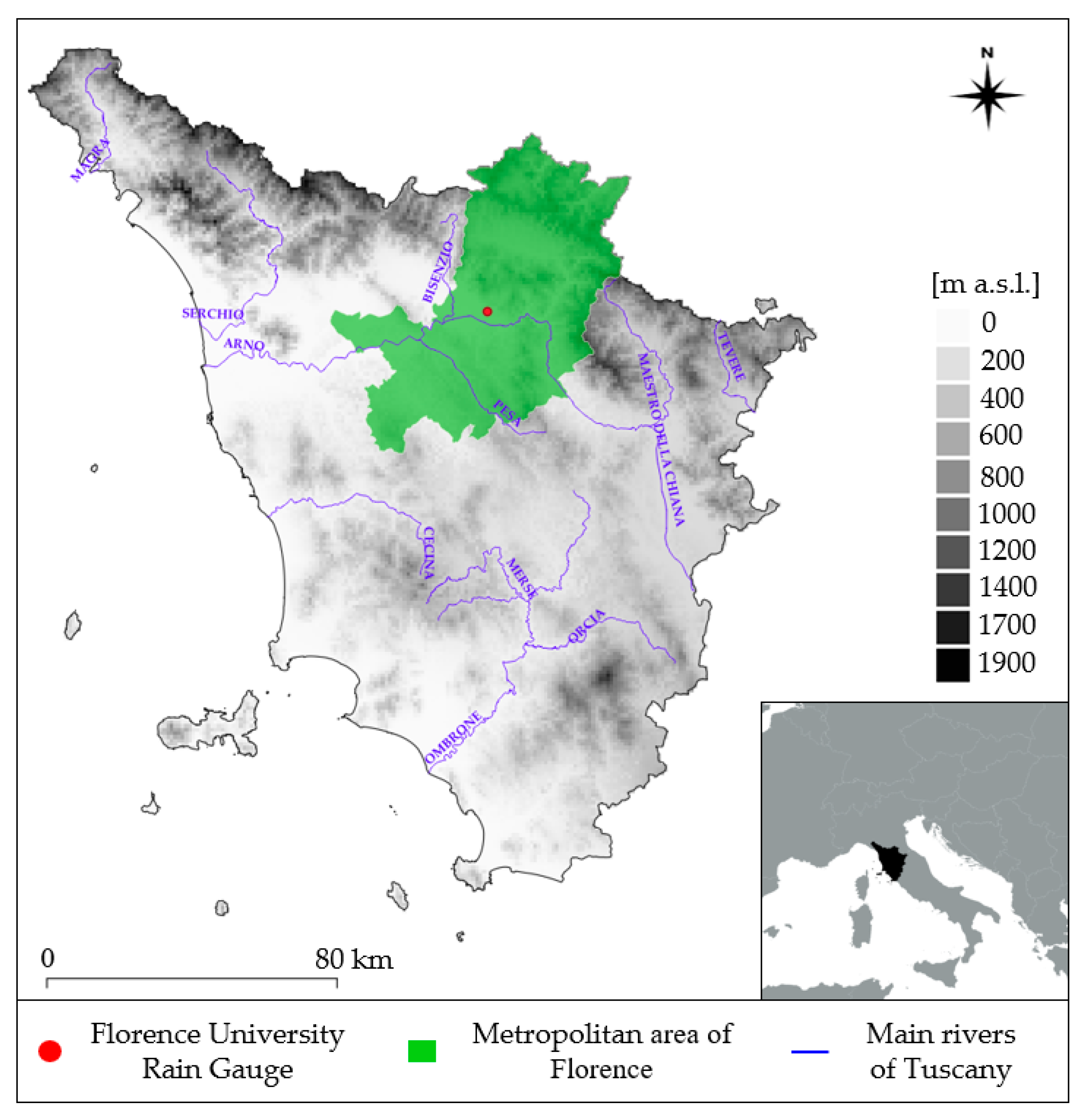
The automatic rain-gauge “Florence University” (id. TOS01001096) was selected as case study (Figure 1). The rain gauge is located at School of Engineering—University of Florence (Tuscany, Italy), at an altitude of 84 m a.s.l. Its coordinates are E 1681124, N 4852004 (EPSG 3003 Monte Mario/Italy zone 1). Observed rainfall data of 20 years, from 1998 to 2018, with temporal aggregation 15 min, were collected and subsequently aggregated with time-step 24 h. The pluviography measurements have a minimum resolution of 0.2 mm. All rainfall data are recorded by the regional monitoring network and archived by the Hydrological Service of Tuscany Region—SIR. Florence experiences a humid subtropical climate characterized by hot sunny, moderately dry summers and mildly cool, rainy winters. The average annual precipitation is 864 mm.
The main objectives of this study can be summarized as follows. First, to analyze the ability of the synthetic rainfall generation process to reproduce the main characteristics of the observed rainfall and the estimation of the hydrologic parameters often used for SuDS design and by using the generally available daily rainfall data; the second aim is focused on the analysis of the effects of storm definition variables on the SuDS design parameter determination.
The following steps schematizes the applied methodology:
- Aggregation of observed 15-min rainfall into a time-step of 24 h. Consequently, two observed rainfall series with different time aggregation were obtained. This process was done in order to manage the rainfall field information commonly available. Nevertheless, the use of sub-hourly series is crucial to verify the results of disaggregation stochastic methodology;
- Calibration of the stochastic rainfall generator based on the 24 h observed rainfall series. Once the model was calibrated, 100 rainfall series, each of 20 years of continuous data with 15 min time-step, were generated;
- Independent storm events were extracted from each, observed and stochastically generated, rainfall series. We considered different values for the minimum antecedent dry weather period (MIT, Minimum Inter-event Time) and different thresholds of storm event total volume. Then, for every MIT and threshold value, key characteristics were calculated for all rainfall event patterns. The comparison of these characteristics was done for the observed and the median of simulated series in order to verify the ability of the stochastic rainfall generator to reproduce the observed rainfall properties;
- Determination of hydrological design parameters of SuDS associated to the storms extracted, considering the different values of MIT and threshold, from each observed and simulated rainfall series. These parameters are usually based on percentiles of rainfall to be managed. These percentiles may be formulated in terms of the number of rainfall events to be managed, Nx or the accumulated volume of the rainfall series to be managed, Vx. Sub-index x refers to the percentage (number or volume) to be managed, commonly used in the practice;
- Two distinct sensitivity analysis were applied to the values of Nx and Vx. Effects of (a) different MIT values and (b) different storm total volume thresholds, on the rainfall volumetric percentiles values were analyzed;
- Comparison and analysis of the results.
2.1. Generation of Stochastic Rainfall Series
The RainSim V.3 model is a robust and well tested stochastic rainfall generator. This model has already been applied in South-European basins [40]. This model facilitates the generation of continuous stochastic rainfall series using a Spatial Temporal Neyman-Scott Rectangular Pulses process (NSRP). A detailed description of RainSim V.3 can be found in Burton et al. [31,41]. Rainstorm events occurs as a temporal stationary Poisson process, while the distribution of the intensities is Exponential. The generator can be used in single or multi-site versions, depending on the number of rain gauges involved. NSRP processes are able to capture the main observed rainfall time-series statistical characteristics: (i) mean waiting time between adjacent storm origins [hours]; (ii) mean waiting time for rain cell origins after storm origin [hours]; (iii) mean duration of rain cell [hours]; (iv)mean intensity of a single rain cell [mm/h]. RainSim operates in three modes: analysis, fitting and simulation. The procedure applied in this study is composed by four steps:
- Analysis to derive statistics from observed rainfall series with 24 h temporal aggregation;
- Fitting/Model calibration. The single-site version of the model is calibrated by applying the log-parameter Shuffled Complex Evolution (InSCE) [42] algorithm with a convergence criterion. This numerical optimization allows to identify the model parameters such that the simulation best corresponds to a selected set of rainfall statistics for each month: mean (24 h), variance (24 and 48 h), lag-autocorrelation (24 h), dry period probability (24 h with a threshold of 1 mm) and skewness (24 and 48 h). For a single site application of RainSim V.3., five parameters usually adopted in NSRP simulators, were calibrated for every calendar month: λ (1/mean waiting time between adjacent storm origins [1/h]); β (1/mean waiting time for rain cell origins after storm origin [1/h]); η (1/mean duration of rain cell [1/h]); ν (mean number of rain cells per storm [-]); xi (1/mean intensity of a rain cell [h/mm]);
- Simulation, that is, generation of 100 rainfall series of continuous data. Each series is composed by 20 years, with a length equal to that of the observed period (1998–2018), of rainfall data with 15 min time-step;
- Analysis to check whether the simulated time series are consistent with the observed one.
2.2. Identification of Independent Rainstorm Events and Key Characteristics of Rainfall Patterns
Different approaches to extract storm events from a continuous rainfall series can be found in technical literature [37,43]. In this study, we applied an approach based on dry inter event time and a threshold value to define non-zero rainfall. The minimum resolution value of the considered rain gauge (Florence University) is 0.2 mm. Thus, this value was used to set the rainfall threshold. First, by applying this approach, homogeneity among observed and simulated series was achieved. Second, independent rainfall events were extracted from observed and simulated series using the minimum antecedent dry weather period approach (MIT, Minimum Inter-event Time). Antecedent dry weather period can be defined as the time of no-rainfall record in the continuous series, that is, the dry period observed between two consecutive non-zero rainfall records [38,39]. As showed in Figure 2, non-zero rainfall pulses belong to the same storm event only if the durations of the antecedent dry weather periods within it are less of an appropriate value, that is the MIT. Otherwise, the antecedent dry weather period represents the variable to separate the end of previous storm event 1 from the start of the successive 2. Different MIT values have been reported in literature, depending on the field of application [43,44,45]. Here, six values of MIT were selected: 3, 6, 12, 24, 48 and 72 h. These sub-daily MIT values were used only for the rainfall series with 15 min temporal aggregation. For observed series with time-step 24 h, only 24 h multiples were applied. As the daily rainfall is the most commonly available rainfall data, consequently, it is relevant to analyze MIT values equal to 24 h and multiples [26,27,38]. Starting from values of rainfall punctual records within every independent rainstorm event, four key characteristics of the rainstorm event pattern were calculated [21]: (a) total volume, that is, total rainfall depth [mm]; (b) duration of the event [hours]; (c) mean intensity [mm/h]; (d) maximum intensity [mm/h]. Afterwards, storm total volume thresholds were applied systematically to the independent rainstorm events previously individuated. This variable corresponds to the minimum precipitation volume that should be exceeded to have a storm relevant for analysis purposes [46]. A selection of four thresholds for the minimum cumulated rainfall volume of every event were used in this study: 0.2, 0.5, 1 and 2 mm [21,47]. A threshold value equal to 0.2 mm leads to consider the entire rainfall information collected within every rainstorm event. Finally, the extraction of independent rainstorm events from observed and simulated series was conducted. These storm series were characterized by the four mentioned key variables of rainfall and their associated exceedance probability values. This process was done for the different volume thresholds.
2.3. Calculation of Rainfall Volumetric Percentiles for SuDS Design
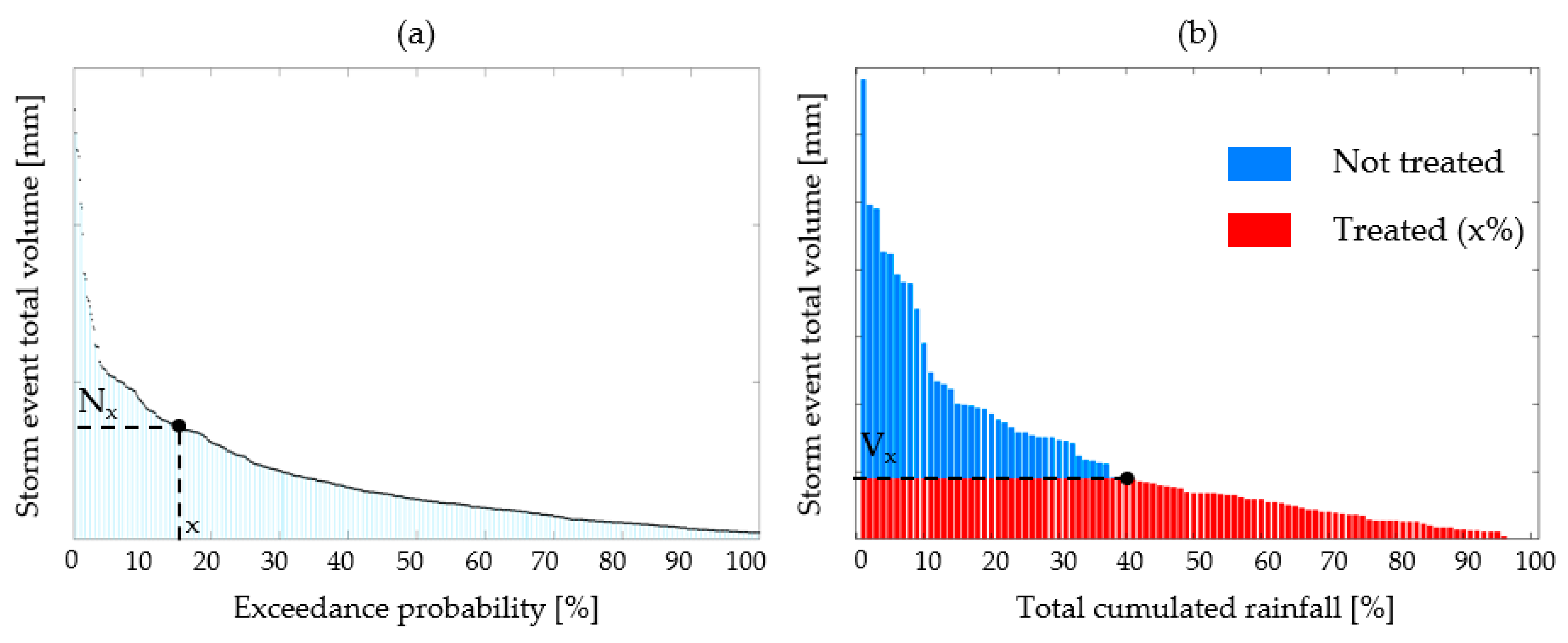
Design of SuDS can be achieved based on rainstorm volumetric percentiles extracted from the analyzed series, observed and simulated. There are various approaches to calculate these percentiles [6,20,22]. Here, hydrological design of SuDS was conducted based on two parameters: (a) those that manage a percentage of the total number of rainfall events, Nx; (b) those that manage a percentage of the total volume of accumulated rainfall series, Vx. Common rainfall percentiles to be managed, to which sub-index x refers, are 80%, 85%, 90%, 95% [6,22]. Rainstorm total volumes were firstly sorted by descending order for both procedures. After that, both procedures differ. In one hand, in order to find Nx values, the exceedance probabilities of every sorted storm event were determined and referred to the respective storm rainfall volume. In this case, Nx represents the total volume of a storm event such that it exceeds the (100−x)% of the total number of rainfall events (Figure 3a) [22]. On the other hand, in order to find Vx values, different total volumes of storm events were progressively selected from the highest to the lowest and compared to a threshold y. The selected SuDS facility would be able to manage a maximum volume y in every rainstorm (Figure 3b, sum of red ordinates). Storm total volumes in excess of the value y would not be treated by the facility (Figure 3b, sum of blue ordinates). Vx is the threshold value such that the cumulative value of depths processed by the facility is the x% of total rainfall depth. By using these two different approaches, N80, N85, N90 and N95 values (same for Nx) were calculated for observed and simulated rainfall series, regarding the six aforementioned MIT and four storm volume thresholds values.
2.4. Evaluation of the Stochastic Model Performance
In order to evaluate the effectiveness of the proposed temporal disaggregation methodology, the simulated key characteristics of rainfall were compared with the observed counterparts with 15 min time-step. A comparison between observed key characteristics of rainfall with 24 h and 15 min time-step, was also conducted. The evaluations of errors were done through the calculation of three statistical indices: mean absolute error (MAE), root mean square error-observations standard deviation ratio (RSR) [48] and Percent Bias (PBIAS) [49].
where n is the number of coupled points used for the evaluations, and are the simulated and observed punctual key characteristics of rainfall, RMSE is the root mean square error and is the standard deviation of the observed data. is the mean of the observed values.
2.5. Limitations of the Methodology
The main limitations of this research lie in the use: (i) of a single rain gauge and dataset; (ii) of a dataset with relatively short length and only valid for very frequent and common rainstorm events, not for heavy and extreme ones; (iii) of a unique stochastic rainfall generator model to simulate sub-daily rainfall records starting from observed data; (iv) of rainfall volumetric percentiles (Nx and Vx) that are suitable for hydrological design of some type of SuDS facilities but not for others. Nevertheless, the effects of temporal disaggregation models as well as different MIT and storm volume threshold values on SuDS types that need different hydrological design parameters, are not considered in this study. These points may limit generalizations of the results and conclusions. Moreover, the methodology did not consider climate change effects or possible long-term variations of the rainfall, that is, the rainfall series generated with the stochastic model do not account for non-stationarity [50]. Despite these limitations, the proposed methodology may provide a useful tool for hydrological design of SuDS. Additionally, SuDS are usually designed for frequent storms, as in the case studied here but not for extreme events.
3. Results and Discussion
3.1. Key Characteristics of Rainfall Series
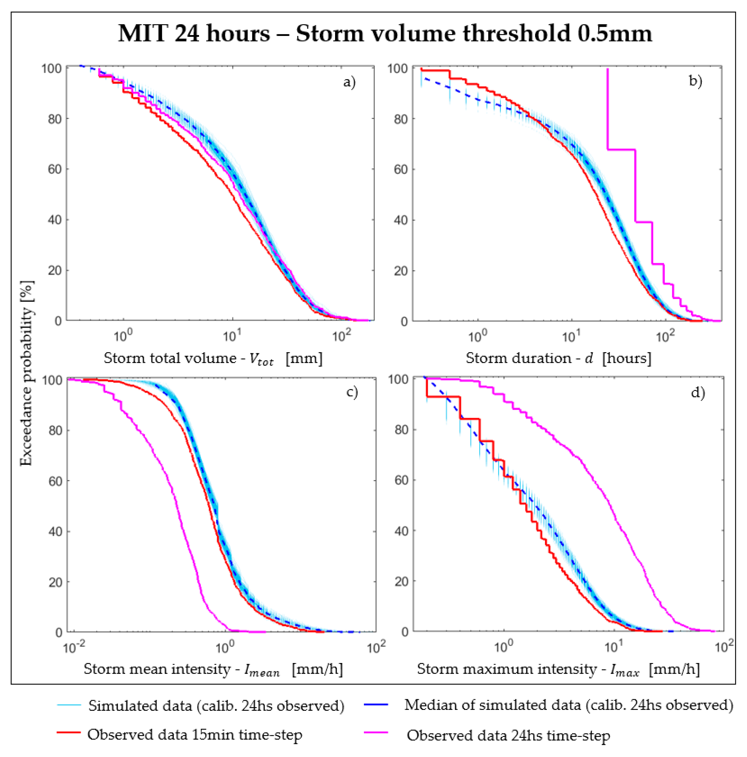
The ability of the stochastic model to reproduce observed rainfall series with n-minutes temporal aggregation was analyzed by comparing key characteristics of the precipitation. The results are shown in Figure 4, which compares the key characteristics derived from three rainfall sources: (i) observed series with 15 min time-step (red lines); (ii) observed series constructed by aggregating observed 15 min time-step to 24 h aggregation time (magenta lines); (iii) 100 stochastic simulated rainfall series and its median value (light blue and dashed blue lines correspondingly). These series were generated at 15 min time step from the model calibrated with observed series aggregated to 24-h time step. The rainfall characteristics analyzed in Figure 4 are: (a) storm total volume [mm], Figure 4a; (b) storm event duration [hours], Figure 4b; (c) storm mean intensity [mm/h], Figure 4c; and (d) storm maximum intensity [mm/h], Figure 4d. Since one objective of this study is to demonstrate the ability of RainSim V.3 to produce better key characteristics of sub-daily rainfall than observed rainfall series with daily time-step, a 24 h MIT value was chosen. Indeed, daily data are the most common data available all over the world. It should be noted that MIT and storm volume threshold values used during calculation of independent rainstorm events, also depend on the type of SuDS, according on their geometry, vegetation percentage and treatment purposes [38]. In addition, Table 1 presents the total amount of rainfall volume, along the entire series (20 years), that is neglected by selecting different MIT and thresholds. It could be seen that influence of the threshold and MIT selected on the total volume considered for the analysis is negligible.
In this analysis, we assumed 0.5 mm as storm volume threshold value. Furthermore, by applying Restrepo-Posada and Eagleson methodology [37] and using a storm volume threshold of 0.5 mm, an MIT equal to 22 h was obtained. This result strengthens the selection of 24 h for the MIT. Table 2 shows results of MAE, RSR and PBIAS statistical indices, calculated applying Equations (1)–(3), using errors between key characteristics of median simulated data and observed data with 15 min time-step, as well as errors between key characteristics of observed daily data and observed 15 min data. Using a MIT equal to 24 h and a storm volume threshold of 0.5 mm, it can be noticed that the median of simulated data improves the values of every statistical index and every key characteristics of rainfall, compared with observed data with 24 h time-step. Except for storm total volume, where a small decrease of simulated indices is detected, the other simulated MAE and RSR values show a substantial decrease in terms of mean errors. Therefore, the stochastic approach improves the values of key characteristics of rainfall compared with observed ones with 24 h time-step. In addition, in order to adjust the simulated and observed key characteristics of the rainfall series, we modified the MIT to different intra-day values. It should be noted that, in the professional practice, where only daily rainfall data are available, SuDS design considering MITs smaller than daily time-step is not possible. Thus, the use of a stochastic rainfall generator enables the use and analysis of sub-daily MIT. Moreover, different sub-daily MIT values were explored to analyze if simulated key characteristics became closer to the ones obtained from the observed series. Figure 5 shows the key characteristics of the rainfall series by considering MIT equal to 12 h. In addition, in Table 2, the three statistical indices were also calculated using a storm volume threshold of 0.5 mm and a MIT equal to 12 h. Results show that this procedure (MIT 12 h, threshold 0.5 mm) improves the values of the statistical indices compared with MIT of 24 h, except for the storm mean intensity.
We calculated the number of rainstorm events associated with a fixed storm volume threshold of 0.5 mm and different MIT values for simulated and observed series. Results of this procedure are reported in Table 3. Simulated series of rainfall in the range of 12 h produced similar number of rainstorm events compared with observed ones using 15 min rainfall time step.
3.2. Stochastic Representation of Rainfall Volumetric Percentiles for SuDS Design
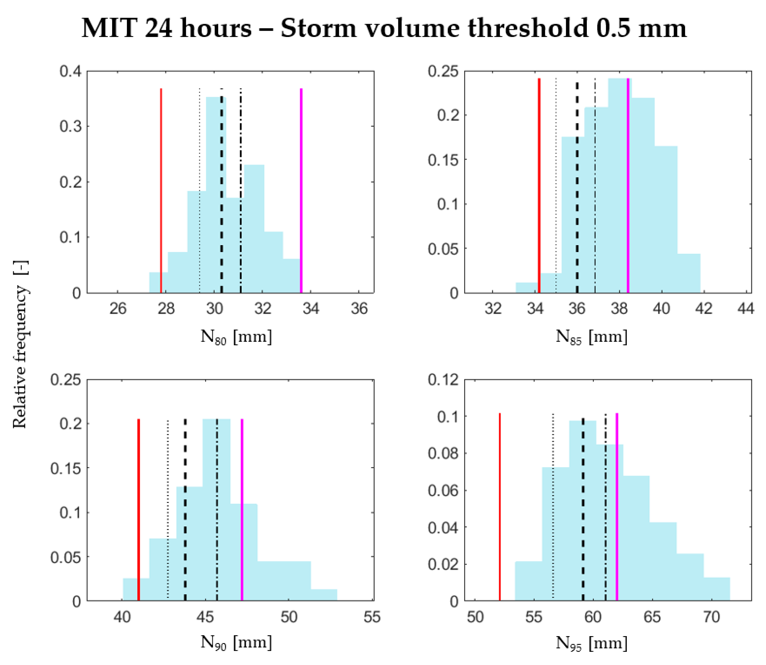
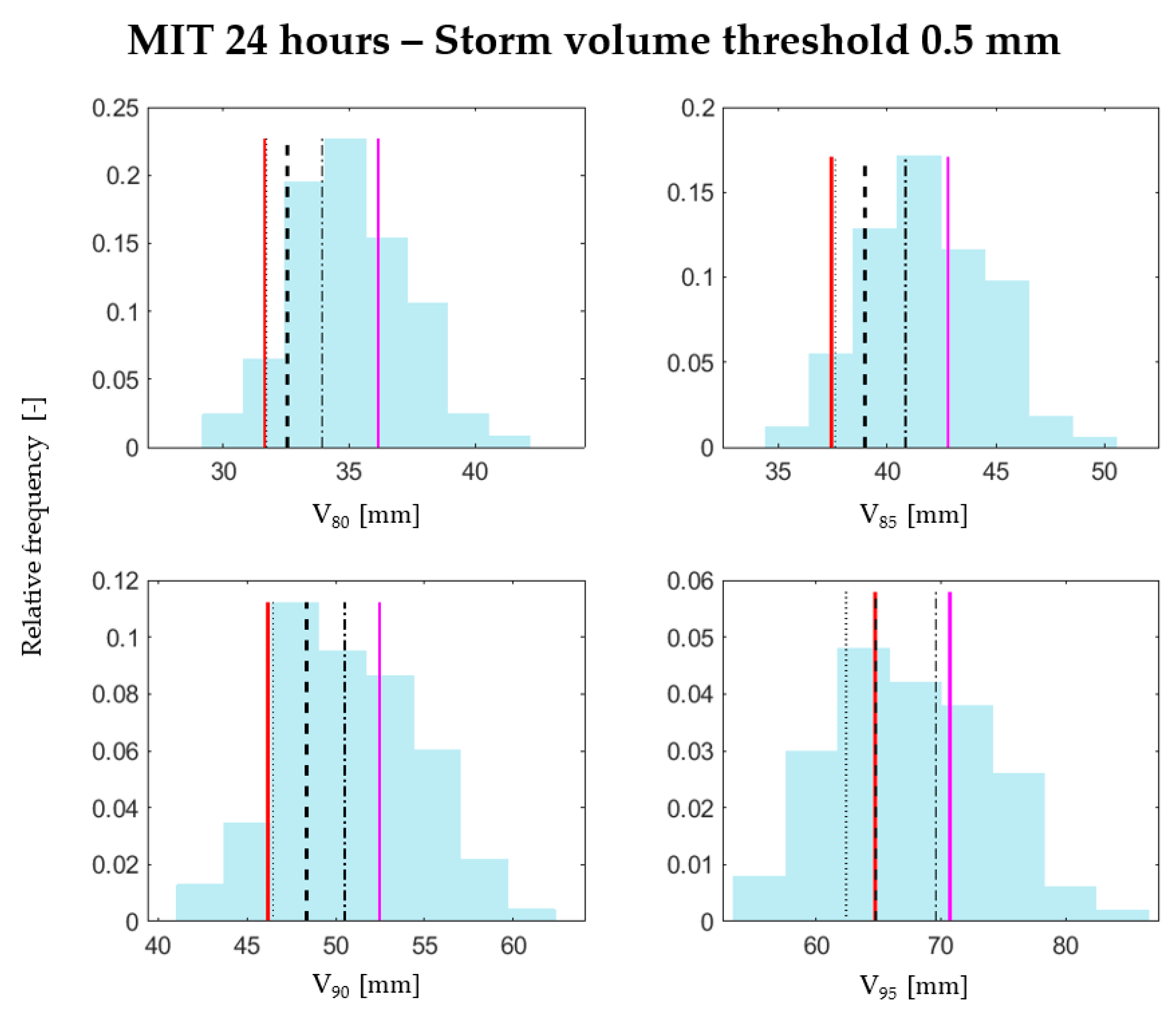
Figure 6 presents the results in terms of relative frequencies of N80, N85, N90 and N95 calculated for MIT 24 h and 0.5 mm storm volume threshold. To create histograms of relative frequencies, values of rainfall percentiles were calculated for each of the 100 simulated rainfall series with 15 min time-step and then grouped in 8 statistical bins according with the Sturges’ rule [51]. Red and magenta lines represent respectively rainfall percentiles of observed series with time-step 15 min and 24 h. As can be seen, the 25th and the 75th percentiles of the distribution of simulated volumetric percentiles are systematically closer to the volumetric percentiles calculated using observed rainfall series with 15 min time-step than to those using observed values with 24 h time-step. For instance, considering the N80 percentiles of Figure 6, the 15-min observed value is 27.9 mm, the 25th and 75th simulated values are 29.4 mm and 31.1 mm respectively (median 30.3 mm), while the observed value with 24 h time-step is 33.6 mm. Moreover, the aforementioned median values are always greater than values of percentiles of observed series with 15 min time-step, being the hydrological design on the safe side. Therefore, for the Florence rain gauge in the period under analysis, the stochastic rainfall generation of sub-hourly rainfall series by using observed daily rainfall, produce design parameters for SuDS more reliable than using directly observed 24 h data. Similar results and considerations were obtained when calculating the relative frequencies of V80, V85, V90 and V95 (Figure 7).
3.3. Sensitivity Analysis of Hydrologic Design Parameters by Considering Different MIT and Threshold Values
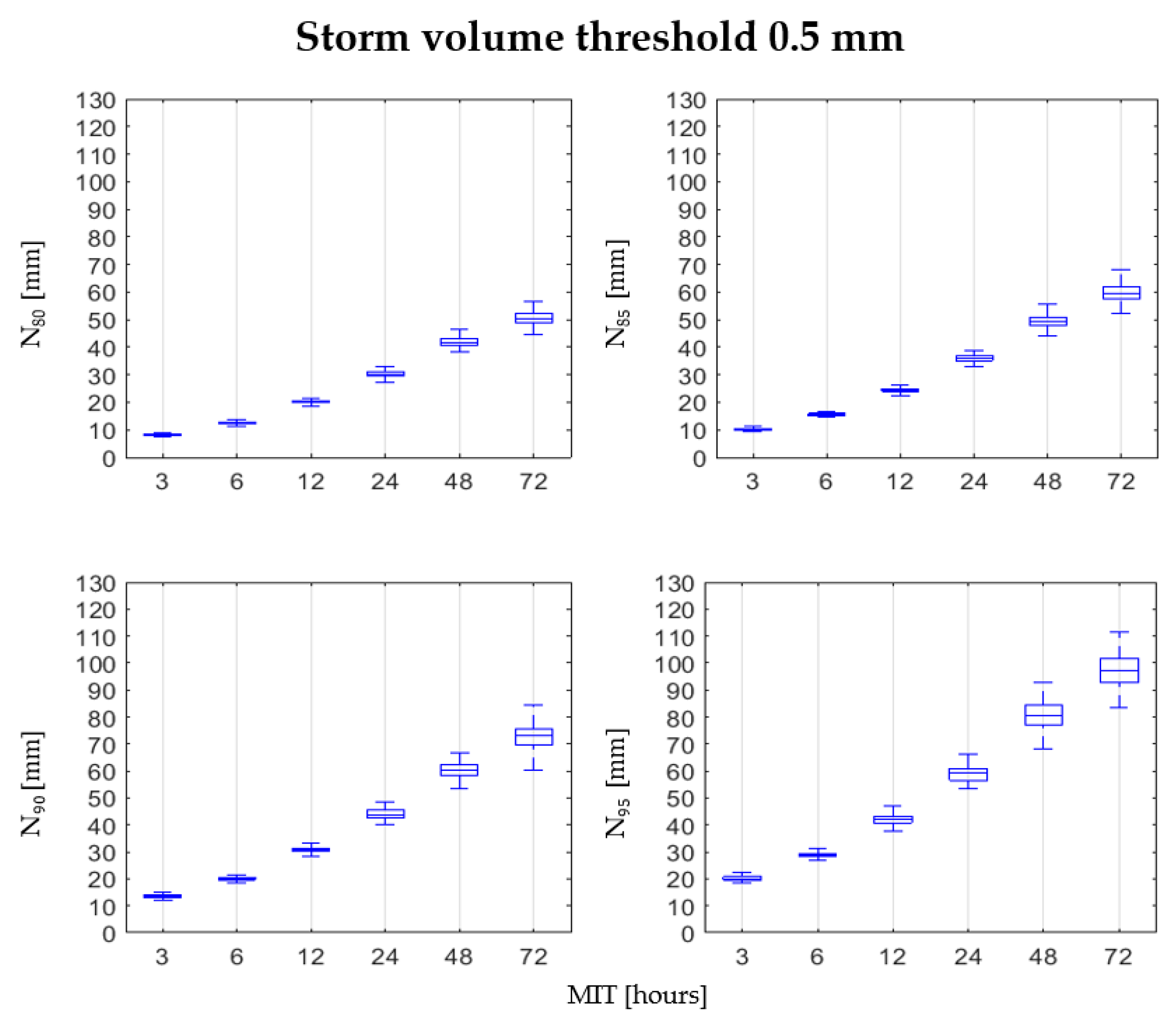
The proposed stochastic disaggregation methodology permits to perform analyses at fine time resolution. Consequently, sub-daily and sub-hourly MIT values can be considered. Therefore, we tested the sensitivity of the calculation of SuDS design parameters based on stochastic rainfall simulation by using different MIT values (assuming a storm volume threshold of 0.5 mm): 3, 6, 12, 24, 48 and 72 h. In addition, we also performed a sensitivity analysis by considering different threshold values (fixing MIT at 24 h): 0.2, 0.5, 1 and 2 mm. In order to assess the sensitivity of Nx (Figure 8) and Vx (Figure 9) to MIT and storm threshold values variation, boxplots were presented for simulated rainfall series. Figure 8 and Figure 9 show the effect of different MIT values on Nx and Vx volumetric percentiles. Both Nx and Vx values are highly sensitive to MIT values. In particular, median values of simulated Nx and Vx percentiles follow a growing trend as the MIT value is increased from 3 to 72 h. The absolute differences among median values of simulated volumetric percentiles when varying MIT from 3 to 72 h are: 42, 49, 59 and 77 mm from N80 to N95, respectively; analogously, 37, 43, 53 and 65 mm ranging from V80 to V95. Considering volumetric percentiles calculated using observed rainfall series with 15 min time-step, the same differences are 37.5, 41.2, 48.8 and 66.4 mm ranging from N80 to N95 and 42.1, 51.6, 69.2 and 102.5 from V80 to V95. It can be also noted that when MIT varies from 3 to 72 h, simulated median values increase by 81%, 82% and 83% when moving respectively from N80 to N95. These results are higher compared with Vx ones, that are respectively 68%, 71% and 72%. For both design parameters, Nx and Vx, larger dispersion is obtained for higher MIT values. In general, this is especially significant for MIT ≥ 24 h. However, this effect is more pronounced for Nx. Regarding these results, Nx provides higher values than Vx and shows higher sensitivity to MIT.
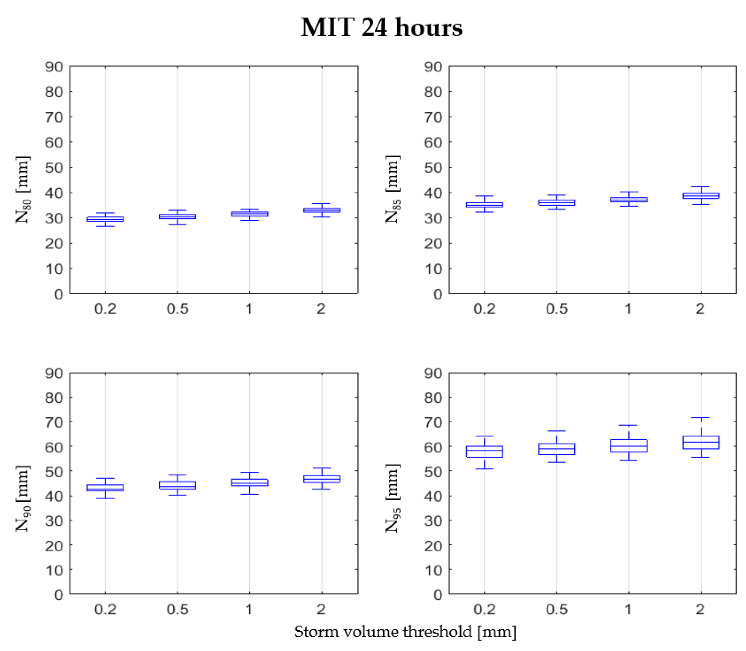
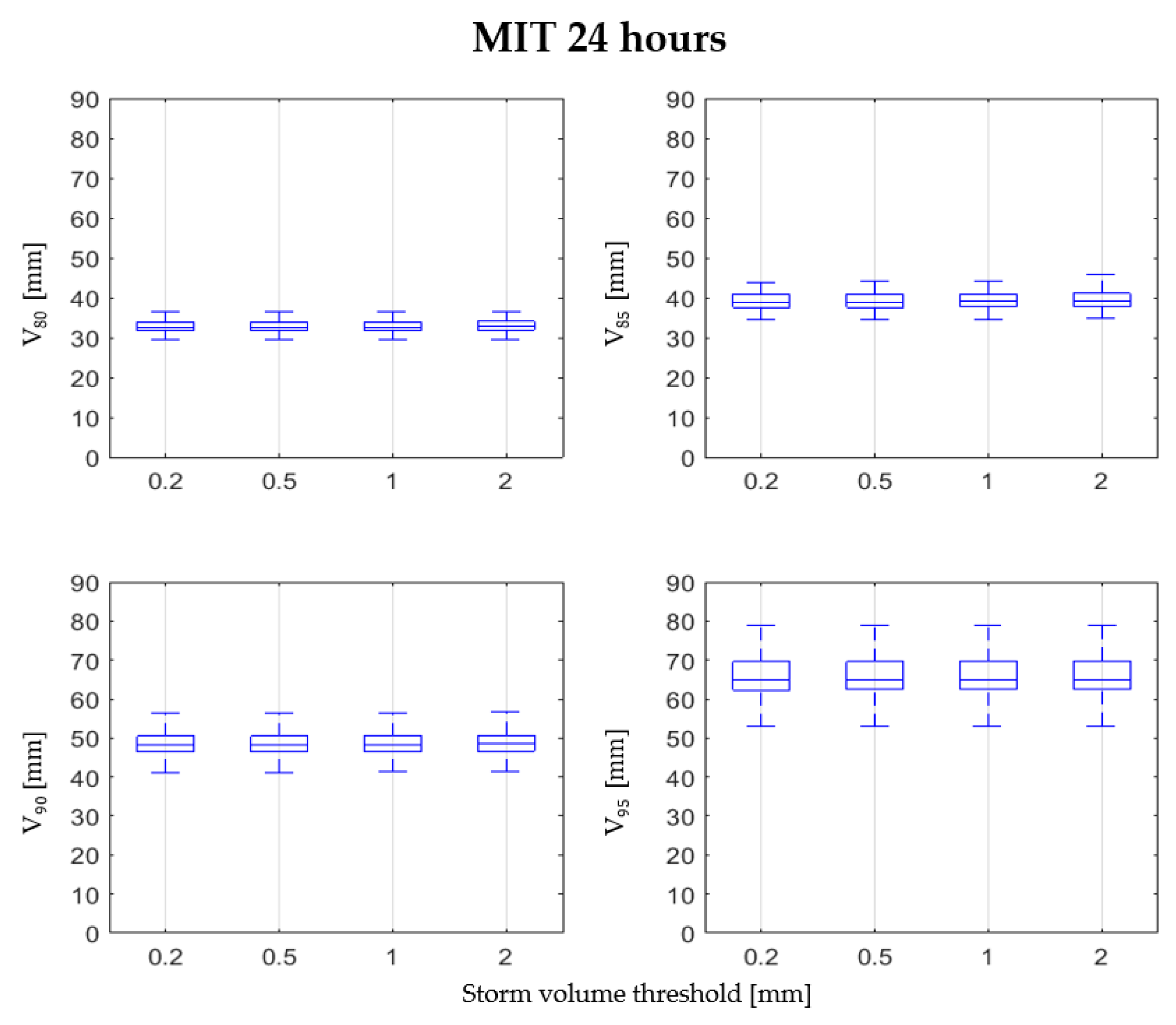
The high sensitivity of Nx and Vx to MIT is to be expected, since the required time to consider two events as independent clearly affects the distribution of relevant storm characteristics, like number of storms or storm depth. This indetermination on the proper value for design parameters may be resolved in two ways. First, we could apply objective criteria to establish the proper MIT value based on the statistical independence of sequential storm events, such as the procedure proposed in [37]. This would lead to an intrinsic design parameter, independent from the element to be designed. The alternative procedure would be based on the expected performance of the element under design. Under this approach, the MIT value chosen for the computation of the design parameter should be, at least, equal to the time required by the element to recover fully operational capability after the previous storm event. For instance, in elements designed to temporarily store a given volume of water, MIT should be at least equal to the time required to empty the water reservoir. This would lead to an element-specific design parameter and the MIT would be established by functional requirements of such element. In accordance with Sordo Ward et al. [21] (rainfall series of Retiro rain gauge located in Madrid, Spain), simulated values of Nx percentiles are conditioned by the storm volume threshold considered (Figure 10), while Vx percentiles are more stable (Figure 11). The median values of simulated Nx percentiles show a growing trend when threshold is altered from 0.2 to 2 mm, while median values of Vx percentiles remain almost constant. As an example, median values of simulated percentile N80 are 29.3, 30.3, 31.5 and 32.9, while V80 values are 32.5, 32.6, 32.6 and 32.7 mm moving from threshold 0.2 mm to 2 mm. The variations of differences between the highest and the lowest values of simulated Nx percentiles in the boxplots are negligible when storm volume threshold increase. Nevertheless, same differences for simulated Vx remain constant. Therefore, simulated median values of Nx percentiles are less sensitive regarding storm volume thresholds than MITs, while simulated median values of Vx percentiles are very sensitive regarding MITs but not sensitive regarding storm volume thresholds. In the case of storm volume threshold, the proper value for design parameters could be based on climate characteristics. The threshold should be set to a value of rainfall depth that is directly evaporated from vegetation or the soil surface, without entering the drainage facilities. With this criterion, humid climates with low potential evapotranspiration would require lower threshold values than dryer climates with high evapotranspiration.
4. Conclusions
In this paper, a temporal disaggregation methodology of daily rainfall records was proposed by using the stochastic spatial-temporal model RainSim V.3. The study provides a methodology to calculate volumetric percentiles Nx and Vx based on definition of independent rainstorm events according to different minimum inter-storm time (MIT) and storm volume threshold values. The ability of the stochastic disaggregation methodology to estimate rainfall volumetric percentiles commonly used in hydrological design of SuDS, was analyzed. The effect of different MIT and storm volume threshold values on simulated rainfall volumetric percentiles was also investigated. The stochastic model was validated based on key characteristics of sub-hourly observed rainfall patterns using three quantitative indices for objective comparison. Despite the obtained results and conclusions are restricted to the selected rain gauge, the study clearly highlights that:
- Using a MIT and a storm volume threshold equal to 24 h and 0.5 mm respectively, simulated sub-hourly rainfall series show better performance than observed daily rainfall for the Florence dataset. Results are compared in terms of key characteristics of rainfall patterns and rainfall volumetric percentiles;
- The stochastic disaggregation model allows the use of sub-hourly MIT values in the process. Therefore, the issue of being able to consider only MIT values equal to 24 h multiples in engineering practice can be overcome. By using a MIT equal to 12 h and a storm volume threshold of 0.5 mm, results in terms of key characteristics of rainfall series and number of rainstorm events, improve comparing with the observed ones obtained with 24 h MIT;
- Nx simulated percentiles are very sensitive to MIT and storm volume threshold values. Consequently, these parameters should be carefully selected to ensure the representativeness of the study. Nevertheless, Vx simulated percentiles show dependence regarding MIT values but not regarding storm volume threshold. These outcomes can be used in the hydrological design of different types of SuDS facilities that deals with different water treatment purposes.
- The proposed methodology produces a probability distribution of design parameters rather than one single deterministic value. This opens the field for doing probabilistic design (for instance, based on percentiles of the design parameters) and for doing uncertainty analysis (by exploring the sensitivity of the design to different values in the probability distribution of the design parameters).
The study of influence of different climates on results using a considerable amount of rain gauge stations, should be the subject of a specific study. Nevertheless, non-stationarity in stochastic generation of rainfall series, considering effects of global warming and climate change, should be considered for future developments.
Author Contributions
Conceptualization, M.P., A.S.-W., P.B. and L.G.; methodology, M.P., A.S.-W., I.G.-M. and L.G.; software, A.S.-W., P.B., I.G.-M.; formal analysis, all authors; investigation, M.P., A.S.-W. and I.G.-M.; resources A.S.-W., E.C. and L.G.; data curation, M.P.; writing—original draft preparation, M.P.; writing—review and editing, all authors; funding acquisition, E.C. and L.G. All authors have read and agreed to the published version of the manuscript.
Funding
This manuscript was supported by funding from: the Spanish Ministry of Science and Innovation (SECA-SRH; Ref. PID2019-105852RA-I00). The first author acknowledges the financial support provided by the International Doctoral program on “Civil and Environmental Engineering,” developed in cooperation among the Italian Universities of Florence, Perugia and Pisa and the T.U. Braunschweig (Germany). M. Pampaloni and E. Caporali were partially supported through the FCRF Grant n. 2018.0967.
Data Availability Statement
Not applicable.
Acknowledgments
The authors wish to thank the Hydrological Service of Tuscany Region for the availability of the dataset. Specific acknowledgments are for the engineers Andrea Fanti and Rodrigo Jodra-Lopez for their valuable participation to the preliminary phases of the research.
Conflicts of Interest
The authors declare no conflict of interest.
References
- Ivanov, D.V. Post-globalization, super-urbanization and prospects of social development. Res. Result. Sociol. Manag. 2020, 6, 72–79. [Google Scholar] [CrossRef]
- Liu, Y.; Engel, B.A.; Flanagan, D.C.; Gitau, M.W.; McMillan, S.K.; Chaubey, I. A review on effectiveness of best management practices in improving hydrology and water quality: Needs and opportunities. Sci. Total Environ. 2017, 601, 580–593. [Google Scholar] [CrossRef]
- Zhou, Q. A review of sustainable urban drainage systems considering the climate change and urbanization impacts. Water 2014, 6, 976–992. [Google Scholar] [CrossRef]
- Raymond, C.M.; Frantzeskaki, N.; Kabisch, N.; Berry, P.; Breil, M.; Nita, M.R.; Geneletti, D.; Calfapietra, C. A framework for assessing and implementing the co-benefits of nature-based solutions in urban areas. Environ. Sci. Policy 2017, 77, 15–24. [Google Scholar] [CrossRef]
- Zhang, D.; Gersberg, R.M.; Ng, W.J.; Tan, S.K. Conventional and decentralized urban stormwater management: A comparison through case studies of Singapore and Berlin, Germany. Urban Water J. 2017, 14, 113–124. [Google Scholar] [CrossRef]
- Ballard Woods, B.; Wilson, B.; Udale-Clarke, H.; Illman, H.; Scott, T.; Ashley, R.; Kellagher, R. The SUDS Manual; CIRIA: London, UK, 2015; ISBN 9780860176978. [Google Scholar]
- Charlesworth, S.M.; Booth, C.A. Sustainable Surface Water Management: A Handbook for SUDS; John Wiley & Sons, Ltd.: New York, NY, USA, 2016. [Google Scholar] [CrossRef]
- Charlesworth, S.M.; Harker, E.; Rickard, S. A Review of Sustainable Drainage System (SUDs): A Soft option for Hard Drainage Questions? JSTOR Geogr. Assoc. 2015, 88, 99–107. [Google Scholar]
- Green, A. Sustainable Drainage Systems (SuDS) in the UK; Springer: Cham, Switzerland, 2019; ISBN 9783030118181. [Google Scholar]
- Sörensen, J.; Persson, A.; Sternudd, C.; Aspegren, H.; Nilsson, J.; Nordström, J.; Jönsson, K.; Mottaghi, M.; Becker, P.; Pilesjö, P.; et al. Re-thinking urban flood management-time for a regime shift. Water 2016, 8, 332. [Google Scholar] [CrossRef] [Green Version]
- Morales, J.A.; Cristancho, M.A.; Baquero-Rodríguez, G.A. Trends in the design, construction and operation of green roofs to improve the rainwater quality. State Art Ingeniería Agua 2017, 21, 179–196. [Google Scholar] [CrossRef] [Green Version]
- Huber, W.C.; Dickinson, R.E. Storm Water Management Model, Version4: User’s Manual; EPA/600/3-88/001a; Environmental Protection Agency: Washington, DC, USA, 1992; p. 720. [Google Scholar]
- Andersen, S.; Maria, S.; Danielsen, H.J.; Andersen, J.S.; Lerer, S.M.; Danielsen, H.J.; Backhaus, A.; Jensen, M.B. Characteristic Rain Events—A tool to enhance amenity values in SUDS-design. Aide à la Décision/Decis. Mak. 2016, 9, 1–4. [Google Scholar]
- Gulliver, J.S.; Anderson, J.L.; Asleson, B.C.; Baker, L.A.; Erickson, A.J.; Hozalski, R.M.; Mohseni, O.; Nieber, J.L.; Riter, T.; Weiss, P.; et al. Assessment of Stormwater Best Management Practices; Report University of Minnesota; University of Minnesota: Minneapolis, MN, USA, 2008. [Google Scholar]
- Rivard, G. Small Storm Hydrology and BMP Modeling with SWMM5. J. Water Manag. Modeling 2010, R236-10. [Google Scholar] [CrossRef] [Green Version]
- Pitt, R.E. Small Storm Hydrology and Why it is Important for the Design of Stormwater Control Practices. J. Water Manag. Modeling 1999, R204-04. [Google Scholar] [CrossRef] [Green Version]
- Fratini, C.F.; Geldof, G.D.; Kluck, J.; Mikkelsen, P.S. Three Points Approach (3PA) for urban flood risk management: A tool to support climate change adaptation through transdisciplinarity and multifunctionality. Urban Water J. 2012, 9, 317–331. [Google Scholar] [CrossRef] [Green Version]
- Geldof, D.G.; Kluck, J. The Three Points Approach. In Proceedings of the 11th ICUD–International Conference on Urban Drainage, Edinburgh, UK, 31 August–5 September 2008. [Google Scholar]
- Damodaram, C.; Giacomoni, M.H.; Prakash Khedun, C.; Holmes, H.; Ryan, A.; Saour, W.; Zechman, E.M. Simulation of combined best management practices and low impact development for sustainable stormwater management. J. Am. Water Resour. Assoc. 2010, 46, 907–918. [Google Scholar] [CrossRef]
- City of Portland. Stormwater Management Manual; Portland Bureau of Environmental Services: Portland, OR, USA, 2016. [Google Scholar]
- Sordo-ward, A.; Gabriel-martin, I.; Perales-Momparler, S.; Garrote, L. Influencia de la precipitación en el diseño de SUDS. Revista de Obras Públicas: Organo profesional de los ingenieros de caminos. Canales y Puertos 2019, 166, 28–31. [Google Scholar]
- Hirschman, D.J.; Kosco, J. Managing Stormwater in Your Community a Guide for Building an Effective Post-Construction Program; No: 833-R-08-001; Environmental Protection Agency, Center for Water-shed Protection; EPA: Washington, DC, USA, 2008. [Google Scholar]
- Paquet, E.; Garavaglia, F.; Garçon, R.; Gailhard, J. The SCHADEX method: A semi-continuous rainfall-runoff simulation for extreme flood estimation. J. Hydrol. 2013, 495, 23–37. [Google Scholar] [CrossRef]
- Guo, Y. Hydrologic design of urban flood control detention ponds. J. Hydrol. Eng. 2001, 6, 472–479. [Google Scholar] [CrossRef]
- Arnbjerg-Nielsen, K.; Willems, P.; Olsson, J.; Beecham, S.; Pathirana, A.; Bülow Gregersen, I.; Madsen, H.; Nguyen, V.T.V. Impacts of climate change on rainfall extremes and urban drainage systems: A review. Water Sci. Technol. 2013, 68, 16–28. [Google Scholar] [CrossRef]
- Brigandì, G.; Aronica, G.T. Generation of sub-hourly rainfall events through a point stochastic rainfall model. Geosciences 2019, 9, 226. [Google Scholar] [CrossRef] [Green Version]
- Sordo-Ward, A.; Bianucci, P.; Garrote, L.; Granados, A. The influence of the annual number of storms on the derivation of the flood frequency curve through event-based simulation. Water 2016, 8, 335. [Google Scholar] [CrossRef] [Green Version]
- Ailliot, P.; Allard, D.; Monbet, V.; Naveau, P.; Ailliot, P.; Allard, D.; Monbet, V.; Naveau, P. Stochastic weather generators: An overview of weather type models Titre: Générateurs stochastiques de condition météorologiques: Une revue des modèles à type de temps. J. la Société Française Stat. 2015, 156, 101–113. [Google Scholar]
- Cowpertwait, P.S.P.; O’Connell, P.E.; Metcalfe, A.V.; Mawdsley, J.A. Stochastic point process modelling of rainfall. I. Single-site fitting and validation. J. Hydrol. 1996, 175, 17–46. [Google Scholar] [CrossRef]
- Rodriguez-Iturbe, I.; Febres De Power, B.; Valdes, J.B. Rectangular pulses point process models for rainfall: Analysis of empirical data. J. Geophys. Res. 1987, 92, 9645–9656. [Google Scholar] [CrossRef]
- Burton, A.; Kilsby, C.G.; Fowler, H.J.; Cowpertwait, P.S.P.; O’Connell, P.E. RainSim: A spatial-temporal stochastic rainfall modelling system. Environ. Model. Softw. 2008, 23, 1356–1369. [Google Scholar] [CrossRef]
- Fowler, H.J.; Kilsby, C.G.; O’Connell, P.E.; Burton, A. A weather-type conditioned multi-site stochastic rainfall model for the generation of scenarios of climatic variability and change. J. Hydrol. 2005, 308, 50–66. [Google Scholar] [CrossRef]
- Cowpertwait, P.S.P. A spatial-temporal point process model with a continuous distribution of storm types. Water Resour. Res. 2010, 46, W12507. [Google Scholar] [CrossRef] [Green Version]
- Wu, S.J.; Tung, Y.K.; Yang, J.C. Stochastic generation of hourly rainstorm events. Stoch. Environ. Res. Risk Assess. 2006, 21, 195–212. [Google Scholar] [CrossRef]
- Wenzel, H.G.; Voorhees, M.L. Evaluation of the Urban Design Storm Concept; Report nr.164; Water Resources Center, University of Illinois: Urbana, IL, USA, 1981. [Google Scholar]
- Bonta, J.V.; Rao, A.R. Factors affecting the identification of independent storm events. J. Hydrol. 1988, 98, 275–293. [Google Scholar] [CrossRef]
- Restrepo-Posada, P.J.; Eagleson, P.S. Identification of independent rainstorms. J. Hydrol. 1982, 55, 303–319. [Google Scholar] [CrossRef]
- Shamsudin, S.; Dan’azumi, S.; Aris, A. Effect of storm separation time on rainfall characteristics-a case study of Johor, Malaysia. Eur. J. Sci. Res. 2010, 45, 162–167. [Google Scholar]
- Balistrocchi, M.; Grossi, G. Predicting the impact of climate change on urban drainage systems in northwestern Italy by a copula-based approach. J. Hydrol. Reg. Stud. 2020, 28, 100670. [Google Scholar] [CrossRef]
- Bianucci, P.; Sordo-Ward, Á.; Moralo, J.; Garrote, L. Probabilistic-multiobjective comparison of user-defined operating rules. case study: Hydropower dam in Spain. Water 2015, 7, 956–974. [Google Scholar] [CrossRef] [Green Version]
- Burton, A.; Fowler, H.J.; Kilsby, C.G.; O’Connell, P.E. A stochastic model for the spatial-temporal simulation of nonhomogeneous rainfall occurrence and amounts. Water Resour. Res. 2010, 46, 1–19. [Google Scholar] [CrossRef] [Green Version]
- Vrugt, J.A.; Gupta, H.V.; Bouten, W.; Sorooshian, S. A Shuffled Complex Evolution Metropolis algorithm for optimization and uncertainty assessment of hydrologic model parameters. Water Resour. Res. 2003, 39, 1201. [Google Scholar] [CrossRef] [Green Version]
- Dunkerley, D. Identifying individual rain events from pluviograph records: A review with analysis of data from an Australian dryland site. Hydrol. Process. Int. J. 2008, 22, 5024–5036. [Google Scholar] [CrossRef]
- Dan, S.; Shamsudin, S.; Aris, A. Modeling the Distribution of Rainfall Intensity using Hourly Data. Fac. Civil Eng. Inst. Environ. Water Resour. Manag. 2010, 6, 238–243. [Google Scholar]
- Walker, S.; Tsubo, M.; Hensley, M. Quantifying risk for water harvesting under semi-arid conditions: Part II. Crop yield simulation. Agric. Water Manag. 2005, 76, 94–107. [Google Scholar] [CrossRef]
- Bacchi, B.; Balistrocchi, M.; Grossi, G. Proposal of a semi-probabilistic approach for storage facility design. Urban Water J. 2008, 5, 195–208. [Google Scholar] [CrossRef]
- Voyde, E.; Fassman, E.; Simcock, R. Hydrology of an extensive living roof under sub-tropical climate conditions in Auckland, New Zealand. J. Hydrol. 2010, 394, 384–395. [Google Scholar] [CrossRef]
- Legates, D.R.; McCabe, G., Jr. Evaluating the use of “goodness-of-fit” measures in hydrologic and hydroclimatic model validation. Water Resour. Res. 2007, 35, 1–9. [Google Scholar] [CrossRef]
- Gupta, H.V.; Sorooshian, S.; Yapo, P.O. Status of automatic calibration for hydrologic models: Comparison with multilevel expert calibration. J. Hydrol. Eng. 1999, 4, 135–143. [Google Scholar] [CrossRef]
- Milly, P.C.D.; Betancourt, J.; Falkenmark, M.; Hirsch, R.M.; Kundzewicz, Z.W.; Lettenmaier, D.P.; Stouffer, R.J. Climate change: Stationarity is dead: Whither water management? Science 2008, 319, 573–574. [Google Scholar] [CrossRef] [PubMed]
- Scott, D.W. Sturges’ rule. Wiley Interdiscip. Rev. Comput. Stat. 2009, 1, 303–306. [Google Scholar] [CrossRef]
Figure 1.
Location of the study case on a Digital Terrain Model (DTM) with a grid resolution of 10 m. The red dot indicates the rainfall gauge location within the Metropolitan Area of Florence.
Figure 1.
Location of the study case on a Digital Terrain Model (DTM) with a grid resolution of 10 m. The red dot indicates the rainfall gauge location within the Metropolitan Area of Florence.

Figure 2.
Identification of independent rainstorm events in a continuous rainfall series. As an example, the calculation of key characteristics of rainfall is showed for storm event 2, composed by five values of single rainfall impulse j.
Figure 2.
Identification of independent rainstorm events in a continuous rainfall series. As an example, the calculation of key characteristics of rainfall is showed for storm event 2, composed by five values of single rainfall impulse j.

Figure 3.
Rainfall percentiles calculated using: (a) the number of rainfall events to be managed, Nx. Black point represents the rainstorm event volume that ensures a treatment of the x% of the number of storm events. (b) the accumulated volume of the rainfall series to be managed, Vx. Sum of red vertical values represents the x% of the total cumulated precipitation of the series, which the Sustainable urban Drainage Systems (SuDS) facility will be able to fully manage. Sum of blue line vertical values represents the total cumulated precipitation unmanaged by the facility.

Figure 4.
Key Characteristics of rainfall pattern calculated using a MIT of 24 h and a storm volume threshold of 0.5 mm: (a) storm total volume [mm]; (b) duration of the storm event [hours]; (c) storm mean intensity [mm/h]; (d) storm maximum intensity [mm/h].
Figure 4.
Key Characteristics of rainfall pattern calculated using a MIT of 24 h and a storm volume threshold of 0.5 mm: (a) storm total volume [mm]; (b) duration of the storm event [hours]; (c) storm mean intensity [mm/h]; (d) storm maximum intensity [mm/h].

Figure 5.
Key Characteristics of rainfall pattern calculated using a MIT of 12 h and a storm volume threshold of 0.5 mm: (a) storm total volume [mm]; (b) duration of the storm event [hours]; (c) storm mean intensity [mm/h]; (d) storm maximum intensity [mm/h].
Figure 5.
Key Characteristics of rainfall pattern calculated using a MIT of 12 h and a storm volume threshold of 0.5 mm: (a) storm total volume [mm]; (b) duration of the storm event [hours]; (c) storm mean intensity [mm/h]; (d) storm maximum intensity [mm/h].

Figure 6.
Relative frequency of volumetric percentiles that treat a percentage of the total number of rainfall events, for MIT 24 h and storm volume threshold 0.5 mm. Red and magenta lines represent respectively observed rainfall series with time-step 15 min and 24-h. Black dashed, dotted and dash-dotted lines represents respectively the median, 25th and 75th percentiles of simulated data (light cyan histograms).

Figure 7.
Relative frequency of volumetric percentiles that treat a percentage of the total volume of accumulated rainfall series, for MIT 24 h and storm volume threshold 0.5 mm. Red and magenta lines represent respectively observed rainfall series with time-step 15 min and 24-h. Black dashed, dotted and dash-dotted lines represents respectively the median, 25th and 75th percentiles of simulated data (light cyan bars).

Figure 8.
Effect of different MITs on values of volumetric percentiles that treat a percentage of the total number of rainfall events, for simulated rainfall series and a fixed 0.5 mm value of storm volume threshold.
Figure 8.
Effect of different MITs on values of volumetric percentiles that treat a percentage of the total number of rainfall events, for simulated rainfall series and a fixed 0.5 mm value of storm volume threshold.

Figure 9.
Effect of different MITs on volumetric percentiles that treat a percentage of the total volume of accumulated rainfall series, for simulated rainfall series and a fixed 0.5 mm value of storm volume threshold.
Figure 9.
Effect of different MITs on volumetric percentiles that treat a percentage of the total volume of accumulated rainfall series, for simulated rainfall series and a fixed 0.5 mm value of storm volume threshold.

Figure 10.
Effect of different storm volume thresholds on values of volumetric percentiles that treat a percentage of the total number of rainfall events, for simulated rainfall series and a fixed 24 h MIT value.
Figure 10.
Effect of different storm volume thresholds on values of volumetric percentiles that treat a percentage of the total number of rainfall events, for simulated rainfall series and a fixed 24 h MIT value.

Figure 11.
Effect of different storm volume thresholds on values of volumetric percentiles that treat a percentage of the total volume of accumulated rainfall series, for simulated rainfall series and a fixed 24 h MIT value.
Figure 11.
Effect of different storm volume thresholds on values of volumetric percentiles that treat a percentage of the total volume of accumulated rainfall series, for simulated rainfall series and a fixed 24 h MIT value.


Table 1.
Percentage of not considered total cumulated rainfall of observed series with 15 min temporal aggregation, depending on Minimum Inter-event Time (MIT) and storm volume thresholds used during the identification of independent rainstorm events.
Table 1.
Percentage of not considered total cumulated rainfall of observed series with 15 min temporal aggregation, depending on Minimum Inter-event Time (MIT) and storm volume thresholds used during the identification of independent rainstorm events.
| Storm Volume Threshold 0.5 mm | Storm Volume Threshold 1 mm | Storm Volume Threshold 2 mm | |||
|---|---|---|---|---|---|
| MIT [hours] | Observed Data 15 min Time-Step | MIT [hours] | Observed Data 15 min Time-Step | MIT [hours] | Observed Data 15 min Time-Step |
| 3 | 1.52% | 3 | 2.65% | 3 | 6.02% |
| 6 | 0.93% | 6 | 1.63% | 6 | 3.96% |
| 12 | 0.58% | 12 | 1.01% | 12 | 2.52% |
| 24 | 0.33% | 24 | 0.57% | 24 | 1.63% |
| 48 | 0.17% | 48 | 0.29% | 48 | 0.85% |
| 72 | 0.11% | 72 | 0.2% | 72 | 0.59% |
Table 2.
Mean absolute error (MAE), root mean square error-observations standard deviation ratio (RSR) and Percent bias (PBIAS) calculated between key characteristics of observed rainfall with 15 min time-step, observed daily (24 h) rainfall and simulated rainfall with 15 min time-step. MIT are fixed to 24 and 12 h.
| MAE [mm] | RSR [-] | PBIAS [-] | |
|---|---|---|---|
| Storm Total Volume | |||
| (MIT 24 h) Observed data 24 h time-step | 2.81 | 0.19 | −16.95 |
| (MIT 24 h) Median of simulated data 15 min time-step | 2.75 | 0.16 | −15.95 |
| (MIT 12 h) Median of simulated data 15 min time-step | 0.44 | 0.09 | −0.57 |
| Storm Duration | |||
| (MIT 24 h) Observed data 24 h time-step | 36.28 | 1.22 | −125.64 |
| (MIT 24 h) Median of simulated data 15 min time-step | 4.36 | 0.16 | −14.33 |
| (MIT 12 h) Median of simulated data 15 min time-step | 1.33 | 0.15 | 0.19 |
| Storm Mean Intensity | |||
| (MIT 24 h) Observed data 24 h time-step | 0.86 | 0.96 | 74.72 |
| (MIT 24 h) Median of simulated data 15 min time-step | 0.35 | 0.59 | −30.71 |
| (MIT 12 h) Median of simulated data 15 min time-step | 0.85 | 0.95 | −60.26 |
| Storm Maximum Intensity | |||
| (MIT 24 h) Observed data 24 h time-step | 9.66 | 4.12 | −361.90 |
| (MIT 24 h) Median of simulated data 15 min time-step | 0.67 | 0.34 | −23.67 |
| (MIT 12 h) Median of simulated data 15 min time-step | 0.48 | 0.29 | −20.27 |
Table 3.
Number of independent rainstorm events calculated using 0.5 mm fixed Storm Volume Threshold and different MIT values.
Table 3.
Number of independent rainstorm events calculated using 0.5 mm fixed Storm Volume Threshold and different MIT values.
| Storm Volume Threshold 0.5 mm | MIT [hours] | |||||
|---|---|---|---|---|---|---|
| 3 | 6 | 12 | 24 | 48 | 72 | |
| Median of simulated data | 2690 | 1904 | 1242 | 828 | 586 | 486 |
| Observed data 15 min. time-step | 2149 | 1718 | 1324 | 1009 | 724 | 558 |
| Observed data 24 h time-step | - | - | - | 663 | 633 | 520 |
Publisher’s Note: MDPI stays neutral with regard to jurisdictional claims in published maps and institutional affiliations. |
© 2021 by the authors. Licensee MDPI, Basel, Switzerland. This article is an open access article distributed under the terms and conditions of the Creative Commons Attribution (CC BY) license (http://creativecommons.org/licenses/by/4.0/).
Share and Cite
MDPI and ACS Style
Pampaloni, M.; Sordo-Ward, A.; Bianucci, P.; Gabriel-Martin, I.; Caporali, E.; Garrote, L. A Stochastic Procedure for Temporal Disaggregation of Daily Rainfall Data in SuDS Design. Water 2021, 13, 403. https://doi.org/10.3390/w13040403
AMA Style
Pampaloni M, Sordo-Ward A, Bianucci P, Gabriel-Martin I, Caporali E, Garrote L. A Stochastic Procedure for Temporal Disaggregation of Daily Rainfall Data in SuDS Design. Water. 2021; 13(4):403. https://doi.org/10.3390/w13040403
Chicago/Turabian StylePampaloni, Matteo, Alvaro Sordo-Ward, Paola Bianucci, Ivan Gabriel-Martin, Enrica Caporali, and Luis Garrote. 2021. "A Stochastic Procedure for Temporal Disaggregation of Daily Rainfall Data in SuDS Design" Water 13, no. 4: 403. https://doi.org/10.3390/w13040403
Note that from the first issue of 2016, this journal uses article numbers instead of page numbers. See further details here.