
Impact of Land Use Change on Non-Point Source Pollution in a Semi-Arid Catchment under Rapid Urbanisation in Bolivia
by
 , ,
, ,
Benjamin Gossweiler
1,2,* ,
,
Ingrid Wesström
2 ,
,
Ingmar Messing
2,
Mauricio Villazón
3 and
Abraham Joel
2 1
Center for Aerospace Surveys and Geographic Information Systems Applications for the Sustainable Development of Natural Resources, San Simon University, P.O. Box 5294, Cochabamba, Bolivia
2
Department of Soil and Environment, Swedish University of Agricultural Sciences, P.O. Box 7014, SE-750 07 Uppsala, Sweden
3
Laboratorio de Hidráulica, San Simon University, P.O. Box 1832, Cochabamba, Bolivia
*
Author to whom correspondence should be addressed.
Water 2021, 13(4), 410; https://doi.org/10.3390/w13040410
Submission received: 15 December 2020
/
Revised: 29 January 2021
/
Accepted: 1 February 2021
/
Published: 4 February 2021
(This article belongs to the Special Issue Impact of Land-Use Changes on Surface Hydrology and Water Quality)
Abstract
:Changes in pollution pressure exerted on the Rocha River in Bolivia from diffuse sources were assessed using potential non-point pollution indexes (PNPI) for 1997 and 2017. PNPI is a simple, low-effort, time- and resource-saving method suitable for data-scarce regions, as it works at catchment level with commonly available geographical data. Land use type (obtained by Landsat imagery classification), runoff (determined by runoff coefficient characterisation) and distance to river network (calculated at perpendicular distance) were each transformed into corresponding indicators to determine their relative importance in generating pollution. Weighted sum, a multi-criteria analysis tool in the GIS environment, was used to combine indicators with weighting values. Different weighting values were assigned to each of the indicators resulting in a set of six equations. The results showed that higher PNPI values corresponded to human settlements with high population density, higher runoff values and shorter distance to river network, while lower PNPI values corresponded to semi-natural land use type, lower runoff coefficient and longer distances to river. PNPI values were positively correlated with measured nitrate and phosphate concentrations at six sub-catchment outlets. The correlation was statistical significant for phosphate in 2017. Maps were produced to identify priority source areas that are more likely to generate pollution, which is important information for future management.
1. Introduction
Water quality degradation is generally caused by non-point sources (storm-water runoff from human settlements and agricultural areas) and point sources (including domestic, industrial and commercial) of wastewater discharge [1,2]. Non-point source pollution (NPSP) is a serious problem world-wide, especially in developing countries [3,4]. It involves addition of impurities to a surface water body or an aquifer, usually through an indirect route and from spatially diffuse sources [5]. Increasing NPSP from expansion of agriculture and urbanisation [6,7] is raising concerns among the scientific community and regulatory agencies [8].
Prevention of NPSP requires an understanding of how particular land uses and other landscape features, such as slope, topography and soil type, influence water quality within a catchment [9,10]. The severity of NPSP is influenced by surface runoff, soil erosion, distance travelled by a pollutant and pollutant transportation, especially immediately after a rainstorm [11]. Surface runoff is a major driving force for NPSP and is primarily responsible for the relationship between land use/land cover and water quality [12,13]. Land use can contribute to polluting a stream by leaching, but it can also act as a filter and keep pollutants from entering the stream by biological trapping [14].
Studies to date on contamination of water bodies have mainly focused on identification of priority source areas (PSAs), i.e., hotspot areas that produce significant pollution, in order to improve NPSP management [15]. Identification of PSAs involves determining the purpose of the evaluation, the scale of the area and data availability, and applying a suitable model [16]. Index-based models may be suitable for this purpose, as they are simple, low-effort and effective. They are especially useful for large-scale analysis where there is a lack of data, as they can easily be produced with limited inputs and variations in local conditions. Such models can also provide a reasonable framework for NPSP assessment at catchment scale, with acceptable accuracy [17]. With accurate PSA identification, water monitoring and restoration programmes for prevention and mitigation of NPSP can be developed.
Potential non-point pollution index (PNPI) is a tool developed by Munafò et al. [18] to assess the overall pressure exerted on rivers and other surface water bodies by land use across any given catchment. It applies a multi-criteria technique, based on expert assessment, to pollutant dynamics. It bypasses the difficulties in representation of the accurate physical reality by assessing pollution potential as a function of indicators, e.g., land use, runoff and distance to the river network. PNPI is based on geographic information system (GIS) at river catchment scale and is designed to inform the scientific community, decision makers and the public about the potential environmental impacts of different land management scenarios [19].
The PNPI tool has been successfully applied in previous studies, e.g., in Italy by Munafò et al. [18] to describe non-point pollution of the Tiber River, by Ciambella et al. [20] to describe the potential contribution of different land uses to non-point pollution of Lake Trasimeno (volcanic ecosystem) and by Cecchi et al. [19] to assess pollution from diffuse sources in Viterbo province, in order to explain the complex interactions between fluvial ecosystems, land use management and environmental health.
The present study was carried out in a 488 km2 catchment in Bolivia prone to soil erosion and undergoing fast and uncontrolled urbanisation. In previous studies [21,22,23], scattered point water samples were taken in the catchment at different time intervals, making it very difficult to track the underlying reasons and location of potential sources of pollution. The objective of this study was to assess the overall pressure of NPSP on the main river, with emphasis on land use changes between 1997 and 2017, using the PNPI approach. Three indicators were considered, related to land use type, runoff potential and distance to river network and their relative importance for NPSP was evaluated. In addition, different weighted factors were tested to identify the best fitting for this particular catchment. The years 1997 and 2017 were chosen because of significant changes in land use and because data on water quality were available for these two years.
2. Materials and Methods
2.1. Study Area
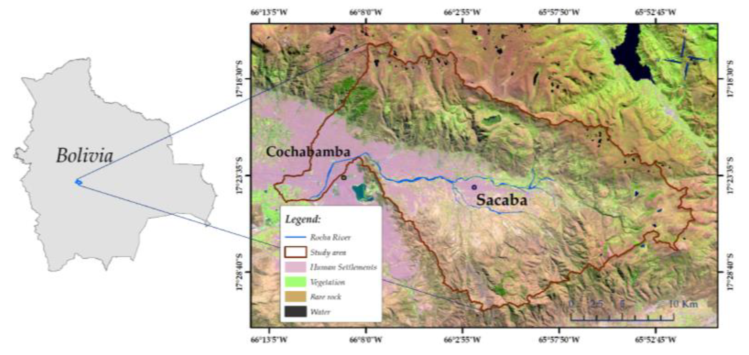
The Rocha River study catchment lies in Cochabamba department in the Highland Valley region in Bolivia, with its outlet at the city of Cochabamba (17°15′36′′ S–17°31′36′′ S; 66°14′02′′ W–65°49′29′′ W) [24] (Figure 1). It consists of the rolling hills, valleys and basins that are part of the Central Cordillera. The geological structure is described in detail by UN-GEOBOL [25], and generally follows a northwest-southeast orientation. The study catchment appears to be the result of deflection of the mountainous chain in the Pliocene and formation of strike slip faults in the Ordovician age [26]. Hydrogeological conditions show unconsolidated porous deposits (alluvial cones, river terraces and fluvio-lacustrine deposits) in the valley plains surrounding the main river and local aquifers (San Benito formation, Catavi and Santa Rosa formation, moraine deposits and Sacaba formation) in the highlands and mountains [27].
The main channel of the Rocha River, which is an important tributary of the Caine River, runs east to west for approximately 80 km. The climate is semi-arid (low precipitation and high potential evaporation) according to data recorded at Aeropuerto-Cochabamba meteorological station (17°24′58′′ S, 66°10′28′′ W, altitude 2548 m) by the Bolivian Service of Meteorology and Hydrology. Median annual temperature in the period 1988–2018 was 17.8 °C and median annual rainfall was 421.2 mm. Rainfall is concentrated in summer (on average 78% of yearly precipitation), during the months December to March, and mostly occurs in short-duration, high-intensity events producing large amounts of runoff. The dry and transition season (May to July) receive 3% and 19% of total annual precipitation, respectively.
In the catchment, mountains, hills, piedmonts and valleys make up the landscape. The altitude ranges between 2500 and 4500 m. In general, soil water permeability is moderately high, organic matter content is low and there is varying abundance of rock fragments in the soil. Soil erosion occurs as rill, pipe and gully erosion. In the piedmont area, the soil types are loam and silt loam [28]. Depositional glacial areas have sandy clay loam soil texture and include locally poorly drained areas. The valley area is characterised by badlands and flatlands of alluvio-lacustrine origin. Fine-textured lacustrine sediments (silty and loamy materials) include isolated gravel channels, lenses and sheets [29]. The valley belongs to the subtropical lower montane thorn steppe ecosystem [30]. Natural vegetation is mostly xeromorphic [31]. Agricultural rain-fed crops include maize, wheat and alfalfa. There are an estimated 500–900 hectares of irrigated cropland in the catchment, mainly potatoes and various vegetables, which are irrigated with river water [32].
Sacaba city population was projected to be 196,540 in 2017 and Cochabamba city population 691,970 [33]. These cities have experienced rapid urbanisation and population growth, of 4% and 2%, respectively, between 1997 and 2017, making the catchment the most densely populated in Bolivia. As a consequence of increasing water demand, proper sanitation services, sewerage and water treatment infrastructure have become unresolved issues. Despite the presence of several potential water sources (e.g., Rocha and Tamborada Rivers, mountain lakes, spring zones, confined aquifers and alluvial fans), water is scarce and currently polluted. In the past 30 years, surface water pollution, contamination and their environmental consequences have been assessed in local reports, but these focus on point pollution, rather than on NPSP.
Non-point pollution sources are an increasing concern in the Rocha River catchment due to a growing range of human activities. Discharges of untreated or poorly treated wastewater and storm-water runoff from hard surfaces, which have no specific point of discharge, are eventually deposited into the river network. In the catchment’s human settlements, surface runoff is not adequately connected to the municipal sewerage system. Thus pollutants such as metals, pesticides, hydrocarbons and solvents deposited on impervious surfaces (e.g., roads or pavements) are discharged into drains, where they can be mixed with sewage and then washed into the river. Between 1992 and 2012, the coverage of sanitary sewage systems increased from 11% to 59% in Sacaba and from 51% to 62% in Cochabamba [34]. These increases were concentrated in the main centre of each city. Illegal discharge events are reported to be quite common and affect water quality in the main river and also its many tributaries (59 in Cochabamba and 137 in Sacaba) [35]. The illegal discharges are related to commercial activities (hotels, restaurants, car washing and markets), industrial spills (textiles, tanneries, slaughterhouses, construction, food and beverages) and domestic sewage and farm wastewater (pigs, chicken and bovine livestock).
2.2. River Network and Catchment Delineation
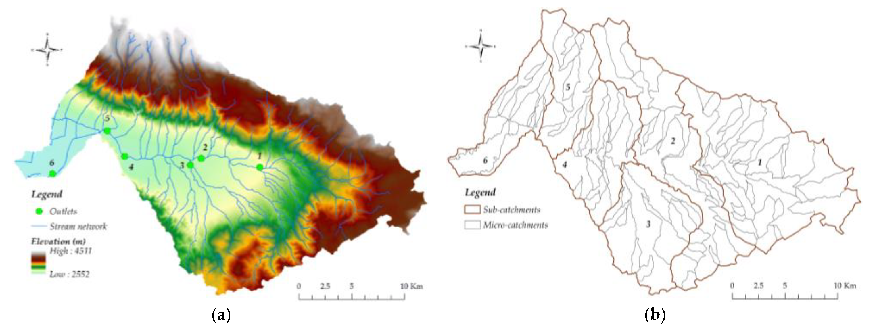
The Shuttle Radar Topography Mission (SRTM) 1 Arc-Second Global Digital Elevation Model (DEM) with 30 m grid spatial resolution was downloaded from https://earthexplorer.usgs.gov/ and re-sized to the study catchment at 1:50,000 scale (Figure 2a). An existing map of the Rocha River stream network, which includes some artificial excavated channels, was downloaded from http://geo.siarh.gob.bo, imported and superimposed onto the DEM to sub-divide the catchment into sub-catchments and micro-catchments (Figure 2b), which were utilised in the PNPI calculations.
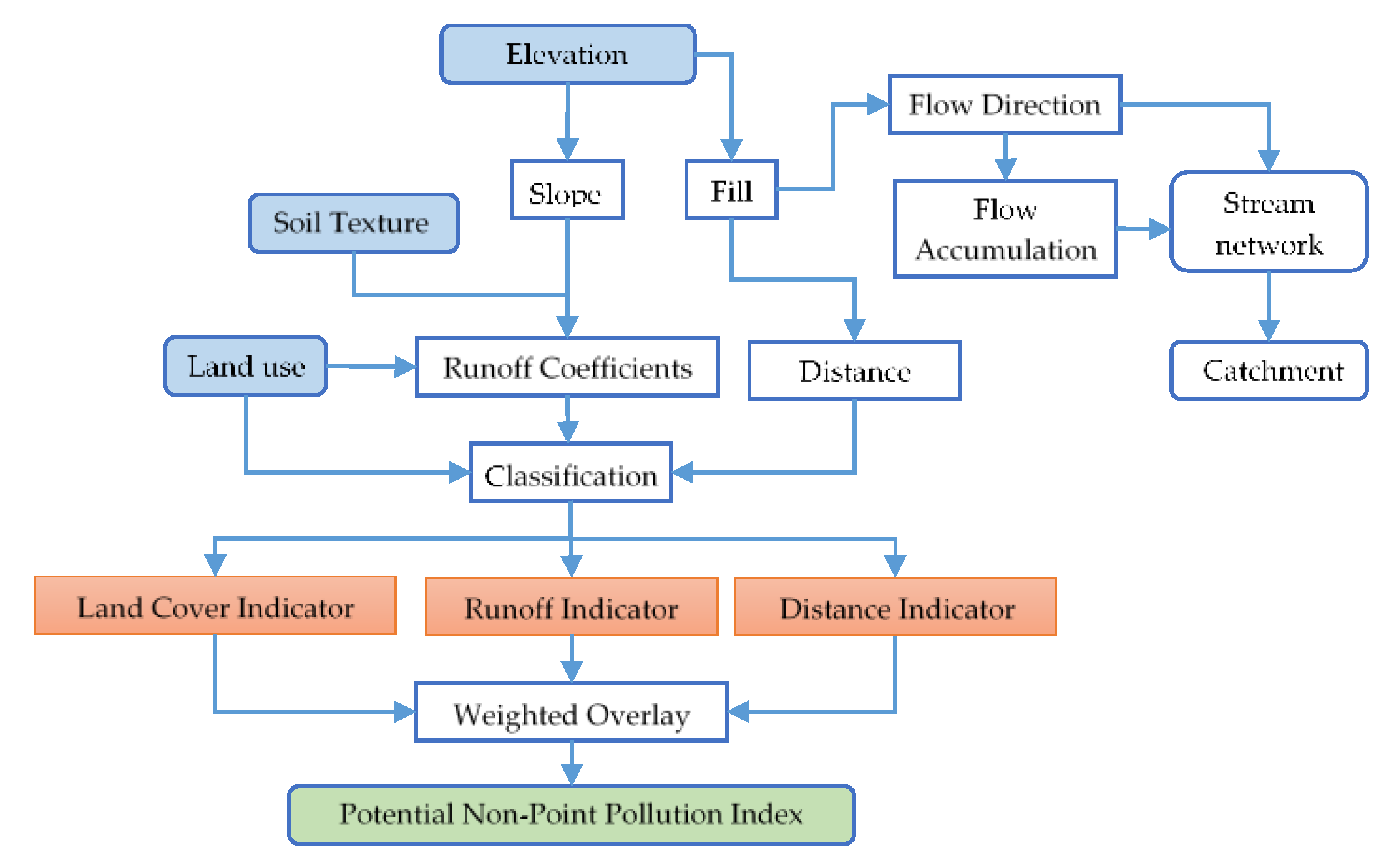
The DEM data were processed by the hydro-processing method proposed by Maathuis and Wang [36] in ArcMap (ArcGIS desktop software, version 10.4; ESRI, Redlands, CA, USA), with the following general steps: (1) filling depressions, (2) calculation of flows (directions, accumulation and length), (3) catchment boundary delineation and (4) sub-catchment and micro-catchment definition. Six delineated sub-catchments (Figure 2b) and their corresponding outlets (1–6 in Figure 2a) were used. These were defined in a previous study by Gossweiler et al. [24] as relevant with regard to topography and land use types in the upstream contributing area. Water flow contribution to each outlet is accumulated from the corresponding upstream sub-catchments. Thus, water flow is accumulated from sub-catchments (Figure 2b) to outlets (Figure 2a) as follows: from sub-catchments 1–6 to outlet 6, from sub-catchments 1–5 to outlet 5, from sub-catchments 1–4 to outlet 4, from sub-catchment 3 to outlet 3, from sub-catchments 1 and 2 to outlet 2, and from sub-catchment 1 to outlet 1.
2.3. Potential Non-Point Pollution Index
The PNPI tool proposed by Munafò et al. [18] assesses pollutant dynamics and water quality (Figure 3). Expert knowledge is incorporated into the PNPI model to allocate values to each indicator, which are used in weighting. Diffuse contamination pressure exerted on water bodies deriving from different land units is expressed in the index as a function of three indicators: land cover (LCI), runoff (RoI) and distance to river network (DI). In this way, potential pollution contribution from different areas and pollutant mobility are determined by the ability of areas to retain and transport water [37].
The PNPI approach has the following advantages: (a) low need for input data and simplicity of use; (b) a GIS environment implementation through ArcMap, generating maps (Geo-Information) that can easily be interpreted to provide decision support (scientists, politicians and public); and (c) a multi-criteria analysis based on expert judgment to evaluate the relative importance of indicators (concerning potential for NPSP generation).
2.3.1. Land Cover Indicator
The land cover indicator (LCI) (Figure 3) represents the potential non-point pollution due to the land uses in a catchment unit [18]. The value of LCI depends on the potential pollution load from a single pixel due to management practices and will vary because of environmental impacts [19]. Determination of LCI requires a geographical location and identification of land use types in the entire catchment. In a previous study, Gossweiler et al. [24] produced a series of land use maps for the Rocha River catchment, from which maps and information for 1997 and 2017 were used in the present study. The land use maps were derived from satellite image interpretation and classification in ArcMap of Landsat 5 Thematic Mapper (TM) of images from 1997 and Landsat 8 Operational Land Imager and Thermal Infrared Sensor (OLI/TIRS) of images from 2017. The classification process was validated only for 2017 classification, since no field data were available for the 1997 classification. Overall accuracy was 78.8% and Kappa statistic was 0.74.
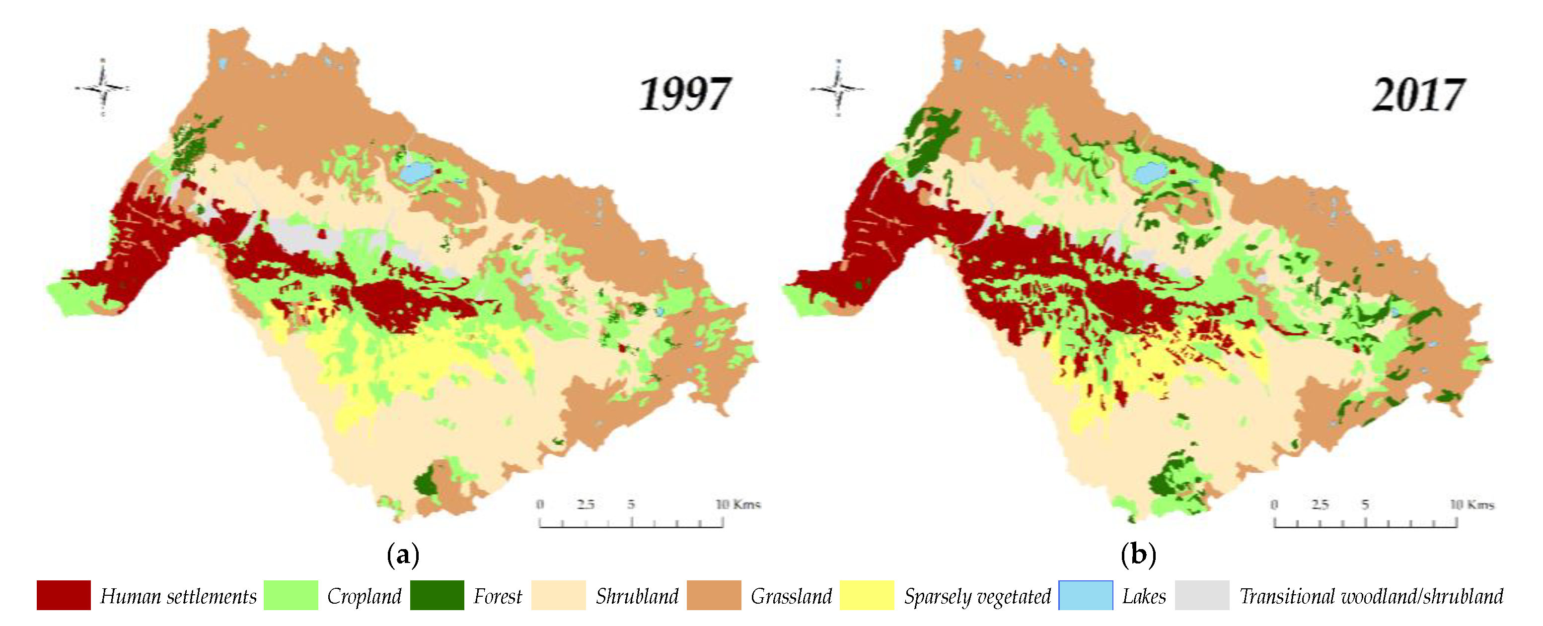
Eight land use types were considered (Figure 4): (i) Human settlements, made up of civil structures or constructed facilities such as buildings and houses, roads and other artificial areas, including vegetated areas (sparse or dense) and bare soil. (ii) Cropland, represented by rain-fed crops (maize, wheat, potato and other native tubers) and irrigated crops (potato, beans, orchard vegetables, alfalfa, oat and barley). Rainfed cropland dominates (74.3% of cropland area) in the catchment, while irrigated cropland (25.7% of cropland area) [38] depends on freshwater irrigation from wells and streams and, to a lesser extent, on wastewater (2.7%) [32]. In general, low rates of chemical fertilisers are used. The main source of plant nutrient is cow manure, followed by poultry manure. An additional source of nutrients is irrigation with untreated wastewater, which can be a source of contaminants (bacteriological, viral and chemical) or a sink. (iii) Forests, composed of several native species (e.g., kewiña, puya, molle, alnus, acacia and quiswara) and exotic species (mostly pine and eucalyptus). (iv) Shrubland, dominated by bushy sclerophyllous vegetation (vegetation with small, hard, thick leaves) and including scattered small trees. (v) Grassland, semi-natural pastures with grazing by several species (e.g., sheep, goats, some cows and llamas in higher parts of the catchment). (vi) Sparsely vegetated areas, dominated by bare soil or very sparse vegetation, which could be susceptible to erosion due to the lack of cover and intense runoff. (vii) Lakes, known as ‘tropical high-altitude mountain lakes’ (exposed to extreme daily temperature variations, intense solar radiation and strong winds), which are located above 3500 m and used for domestic water supply and agriculture. They receive water from rain and runoff from nearby areas and water quality is generally good, with low levels of nitrates and phosphorus (P) [39]. (viii) Transitional woodland/shrubland, consisting of herbaceous vegetation with scattered trees on alluvial fans where water infiltrates through permeable layers of coarse material (boulders, gravel, sand) close to the mountain to finer, permeable sediments in the base of the fans [26]. These fans represent the most important areas for groundwater exploitation and water supply for human settlements.
In high altitudes of the catchment in the north and east partsgrassland and shrubland are dominant land use types. In these areas some forest, lakes and cropland (rain fed crops) are also found. S In lower altitudes, the dominated land uses are human settlements, together with cropland (irrigated and rain-fed crops), transitional woodland/shrubland and sparsely vegetated areas. The distribution of land use types in the Rocha River catchment in 1997 and 2017 is shown in Figure 4.
The land use types (Figure 4) and their corresponding area of cover (Figure 5) were classified in order to obtain LCI. The results showed that human settlements increased in area from 47.7 km2 in 1997 to 76.3 km2 in 2017 (+2.5% in terms of compound annual growth rate, CAGR), reflecting population growth and urban sprawl. At the same time, semi-natural cover (grassland, shrubland, sparsely vegetated areas, transitional woodland/shrubland and lakes decreased (−14.2% CAGR), whereas forest (+6.5% CAGR) and cropland (+0.6% CAGR) increased. There was a clear increase in human settlements in all sub-catchments, but particularly in sub-catchments 6 and 4 (Figure 5; see Figure 2b for sub-catchment numbers). Increases in forest affected sub-catchments 1, 2 and 6 and increases in cropland affected sub-catchments 1 and 5. Decreases in semi-natural land use types mainly affected grassland in sub-catchments 1, 4, 5 and 6, shrubland in sub-catchment 1, transitional woodland/shrubland in sub-catchments 4, 5 and 6, and sparsely vegetated areas in sub-catchments 3 and 4. The decrease in shrubland affected most sub-catchments. Lake cover remained the same between 1997 and 2017, with very low percentage changes.
The well-known relationship described by numerous authors between land use and nitrogen (N) dynamics [40] was used in calculation of LCI in areas affected by humans (human settlements and cropland). The literature on phosphorus (P) emissions from different land uses was also reviewed. The LCI values for human settlements and cropland were related to the N and P loads, while the approach used for other land use types was adapted from the literature as described below.
Human settlements were considered as main contributors to NPSP because they are widespread in the catchment and have very low levels of wastewater treatment. They were considered to produce average emissions of 4.3 kg N and 0.53 kg P per person and year, based on previous studies by Smith et al. [41], Santos et al. [42] and Van Drecht et al. [43] in areas where wastewater is untreated or poorly treated. However, most of the sewage water from Cochabamba city centre (sub-catchment 6 in Figure 2b) is diverted outside the catchment to the municipal water treatment plant, whereas sewage water from Sacaba city is discharged directly into the Rocha River, since no treatment plant is operational or working properly. The N and P emissions given above were multiplied by population data for 1992, 2001 and 2012 [33], and then arranged into population density classes (Table 1). Cropland in the catchment receives manure and some chemical fertilisers providing a total of 29.1 kg N ha−1 year−1 and 13.4 kg P ha−1 year−1.
The LCI values for natural and semi-natural areas (Table 1) were partly adapted from Cecchi et al. [19] and Puccinelli et al. [44], who present data on potential generation of pollution for different land use types as evaluated by specialists. The lowest LCI value (Table 1) was given for lakes, since they can trap transported nutrients and retain potential pollution. Forest, shrubland and grassland were given relatively low LCI values, since they have a cover of native and/or exotic plant species with the capacity to capture/retain pollution. Transitional woodland/shrubland areas were also given a low LCI value, due to their permeable layers of coarse materials. Low to medium LCI values were assigned to cropland and sparsely vegetated areas, with sparsely vegetated areas given a higher value than cropland because of the increased risk of soil erosion. The highest LCI values were assigned to human settlement.
2.3.2. Runoff Indicator
Runoff indicator (RoI) takes into account the potential of water to move as surface runoff. Runoff coefficient (Ci) is a dimensionless factor that is used to convert rainfall amounts into surface runoff [45]. In the present study, RoI was equal to Ci for each pixel along the hydraulic path from pixel to pixel to the six sub-catchment outlets. RoI values were obtained as a function of the interaction between land use (cover) condition, soil texture and slope classes. Maps of land use type, soil texture and slope range were generated and then overlain using the “Intersect” Tool in ArcMap. A geometric intersection of the three maps was generated and the Ci values in Table 2 were set.
Many attempts to define widely accepted Ci values have been made in different studies, but uncertainty still remains. The Ci value used in the present study for cropland was constructed based on tables presented by The Clean Water Team [46], while that for human settlements was based on Schwab et al. [47] as cited by Hudson [48] (Table 2). Runoff coefficient values for slopes exceeding 30% and for human settlements with slopes up to 10% were not included in the original tables. Therefore Ci values proportional to their susceptibility to generate surface runoff were allocated to these areas, based on linear regression between slope ranges and Ci values already defined.
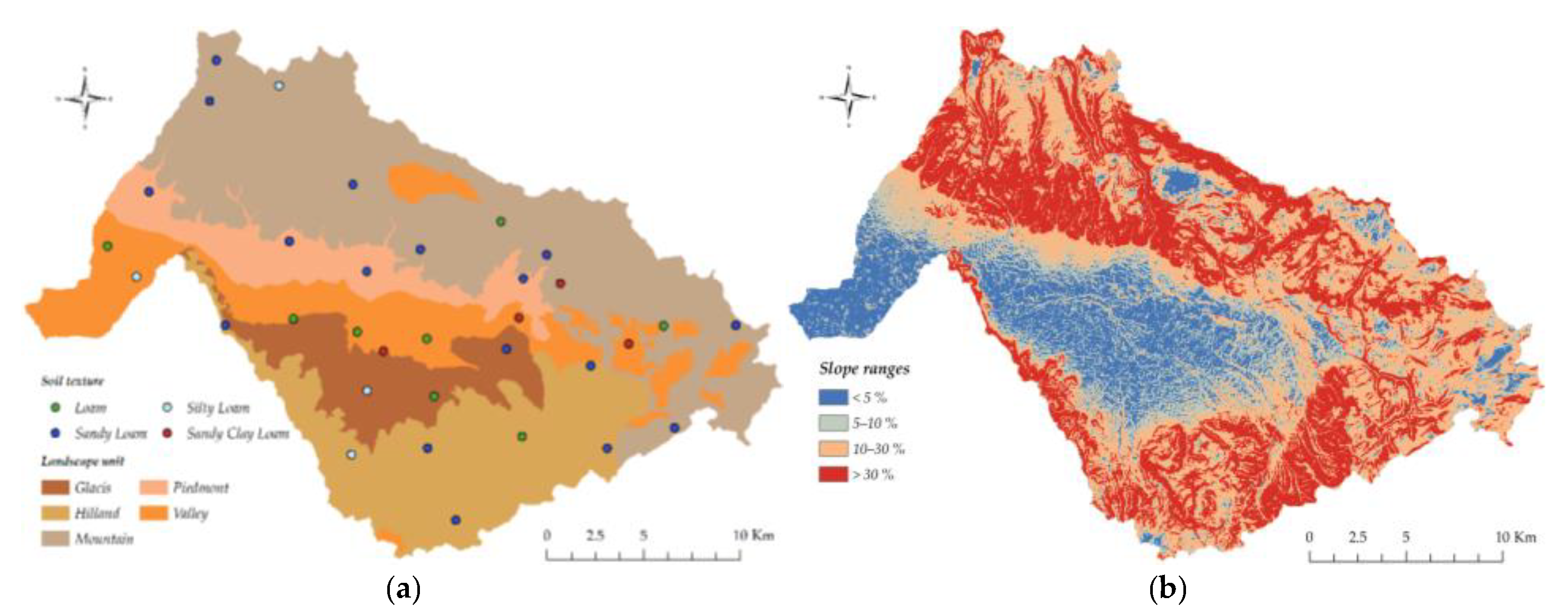
Soil texture information was obtained from a soil dataset constructed with data from the IAO [31], which is based on topsoil (<20 cm) samples analysed by the gravimetric (pipette) method. Soil texture classes (set according to particle fraction distribution of sand, silt and clay) were rearranged into three coarse texture classes (Table 2). The catchment is dominated by sandy loam texture in areas with mountains and hills, whereas in the river valley and nearby areas, loam, silty loam and sandy clay loam are also present (Figure 6a). The texture classes in Schwab et al. [47] were related to landscape units, so that valley and glacial deposits were assigned “>45% sand” (“Open Sandy Loam”) and mountains, hills and piedmont were assigned “clay and silt” (“Clay and Silt Loam”). No part of the landscape was assigned “>55% clay” (“Tight clay”). Thus, a soil texture map for the texture classes shown in Table 2 was produced based on the soil textures and landscape units in Figure 6a. It was spatialised by the geopedological approach [49]. In this context, geomorphological units (mountains, hills, piedmont, glacial deposits and valley) from Metternich [50] provided the contours of the map units (“the container”), while pedology provided the soil textures of the map units (“the content”).
The slope values for each pixel were derived from the DEM. In order to obtain the same slope classes as in Table 2 (i.e., <5%, 5–10%, 10–30% and >30%), the values obtained were classified with the tool “Reclassify” in ArcMap. The dominant slope class was 10–30% (36% of the area), followed by slope > 30% (33% of the area), slope < 5% (17%), and slope 5–10% (14%).
2.3.3. Distance Indicator
Distance indicator (DI) is a coefficient reflecting the mobility of a pollutant [18]. It indicates that the potential impact of pollution decreases with increasing distance from a given pixel to the stream outlet or the river network, due to possible retention on the way to the river network. In the present study, the distances considered to obtain DI were the distance travelled between any given pixel (smallest unit of area) and the closest river network segment. DI was determined as geodesic straight perpendicular (Euclidean) distance (“Near” Tool in ArcMap), in an attempt to simplify the analysis and to avoid additional sources of error.
The calculated distances were rescaled (using the “Reclassify” Tool” in ArcMap) to obtain DI as follows: a) the distance values calculated (min: 0 m and max: 3680.7 m) were sorted in ascending order; b) distances were fitted into 10 classes by the Jenks method [51], where class breaks were determined statistically by finding adjacent feature pairs between which there was a relatively large difference in data value; and (c) each of the 10 classes was assigned a DI value between 0.1 and 1 (see Table 3). A longer distance to the river network gave a lower DI value (towards 0.1) and a shorter distance gave a higher DI value (towards 1). Thus, distances were inversely proportional to DI values, to reflect the decreased effect of pollutants with distance to river (possibly combined with increased travel time) and thereby decreased accumulated pollution percolation (sinks) along the flow path.
The “Reclassify” operation was used to normalise maximum and minimum distance values ranging between 0.1 and 1, so that DI could be combined with the other indicators to obtain PNPI. For that reason, distance intervals calculated are only applicable for the particular study area, so each new study should calculate its own distance intervals. In the present study, DI was the same for both years studied, 1997 and 2017, assuming no changes in stream network.
2.4. PNPI Implementation
Implementation of PNPI was conducted in ArcMap by the weighted sum tool, to create a PNPI map showing PSAs for each pixel of the DEM (smallest unit of surface). Weighted sum is a multi-criteria analysis tool that provides the ability to weight (by relative importance) and combine multiple inputs (representing multiple indicators) to create an integrated analysis [52]:
where k is the total number of indicators, wi is a coefficient of weights for each indicator and xi is the corresponding indicator (LCI, RoI and DI), with values between 0 and 1.
Six set-ups of weighting values were applied for the three indicators, using Equations (2)–(7), to test their effects on generation of diffuse pollution in the study area. LCI was considered the most important indicator, since land cover change is known to be the main cause of NPSP in the catchment. RoI and DI are also closely related to non-point pollution, due to pollutant mobility (dumping) by source of surface runoff and transport distance:
PNPI = LCI*4 + RoI*4 + DI*2
PNPI = LCI*5 + RoI*2 + DI*3
PNPI = LCI*5 + RoI*3 + DI*2
PNPI = LCI*6 + RoI*1 + DI*3
PNPI = LCI*6 + RoI*3 + DI*1
PNPI = LCI*8 + RoI*1 + DI*1
Predefined weighting values based on the rank sum method [53] presented by Munafò et al. [18] were used in Equation (3). The other five Equations (2), (4)–(7) were tested in an attempt to optimise weighting value with regard to local conditions in the catchment. Thus, while LCI weighing values remained highest, due to the local importance of this indicator in the catchment, RoI and DI weighing values varied at lower values.
The micro-catchments (see Figure 2b) were used to summarise PNPI values, in order to provide an applicable understanding of PNPI results in planning management scenarios. The accumulated average PNPI value for each sub-catchment was calculated through zonal statistics in ArcMap (GIS environment) regarding accumulated flows from each micro-catchment. The different PNPI values were aggregated into five classes, the colour code and pollution potential of which are listed in Table 4.
2.5. PNPI Performance Evaluation
Validation of PNPI consisted of comparing values for the water quality parameters nitrate and phosphate, as measured at monitoring stations in the six outlets in 1997 and 2017 (reported in Gossweiler et al. [24]), against PNPI values for each sub-catchment. The nitrate and phosphate concentrations were derived from samples taken only in the dry season, which were analysed at the Water and Environmental Sanitation Center (CASA) laboratory, at San Simon University (Cochabamba, Bolivia) in the two years.
Correlation analyses were performed with the following null hypotheses: (1) Measured nitrate values in the catchment are not related to PNPI values; and (2) measured phosphate values in the catchment are not related to PNPI values. For this purpose, the relationships between nitrate and accumulated average PNPI values, and between phosphate and accumulated average PNPI values, were analysed for correlations using the R statistical software (R Development Core Team 2011) version 3.6.1 (The R foundation, Vienna, Austria).
3. Results
3.1. Land Cover Indicator (LCI)
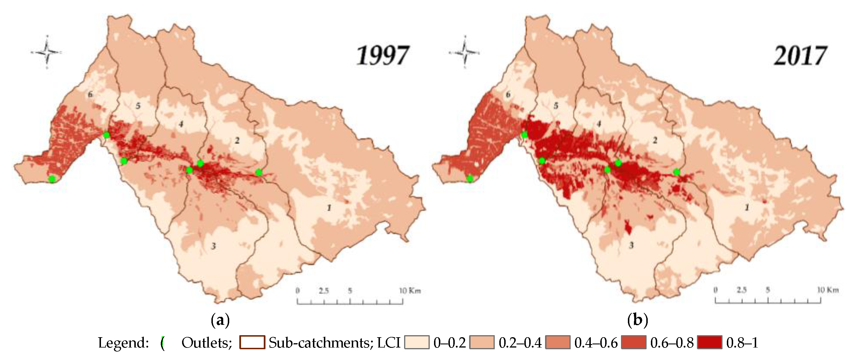
The geographical distribution of LCI in 1997 and 2017 is presented in Figure 7. In general, areas with higher LCI values (LCI 0.6–0.8; 0.8–1, see Table 1) were found to be located mainly in the middle part of the catchment, corresponding to high-density (>100 people per ha) human settlements (see Figure 4). Areas with lower LCI values at higher elevations included grassland, shrubland, transitional woodland/shrubland and forest (LCI 0–0.2), and cropland and sparsely vegetated areas surrounding human settlements (LCI 0.2–0.4). Areas with higher LCI values in 1997 (Figure 7a) covered 6% of the total catchment area, while areas with lower LCI values covered 90%. In 2017, areas with higher LCI values (Figure 7b) increased to occupy 15% of the catchment area, while areas with lower LCI values decreased to 85%. The study catchment was dominated by the LCI class 0.2–0.4 in both 1997 (60% in Figure 7a) and 2017 (52% in Figure 7b).
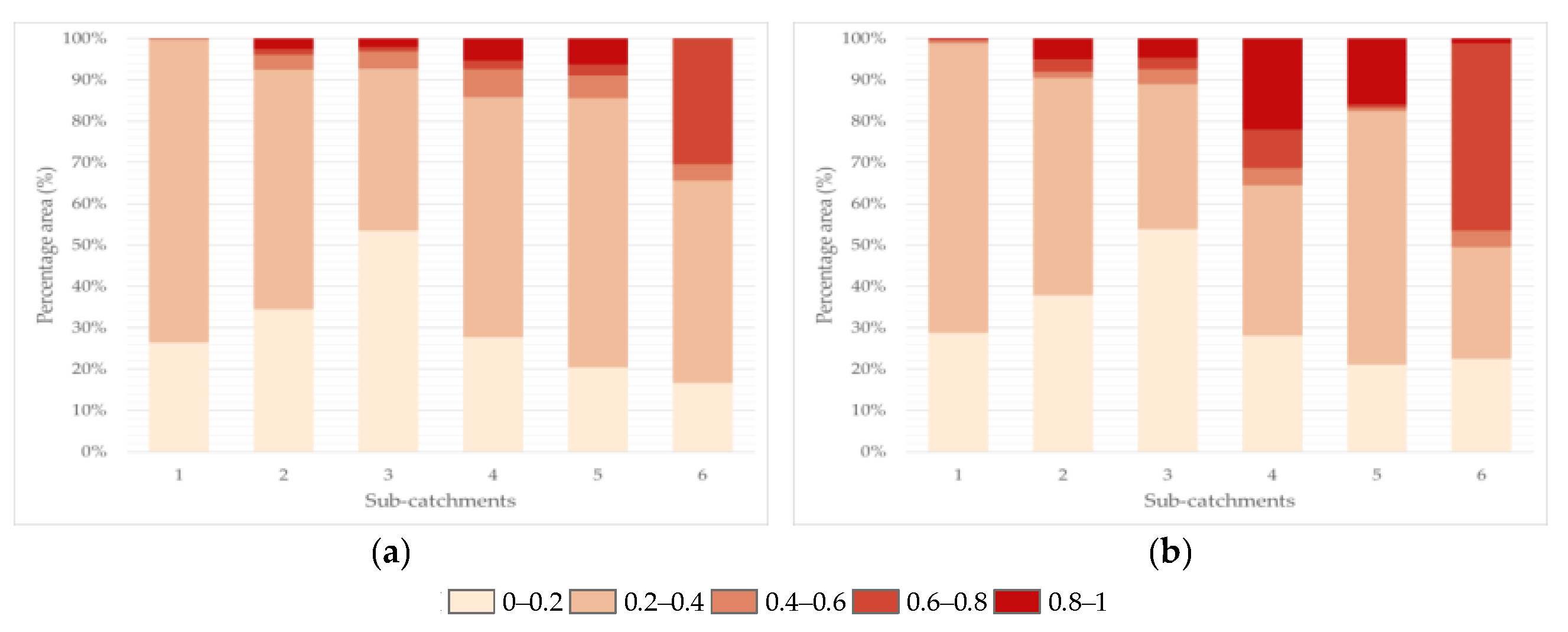
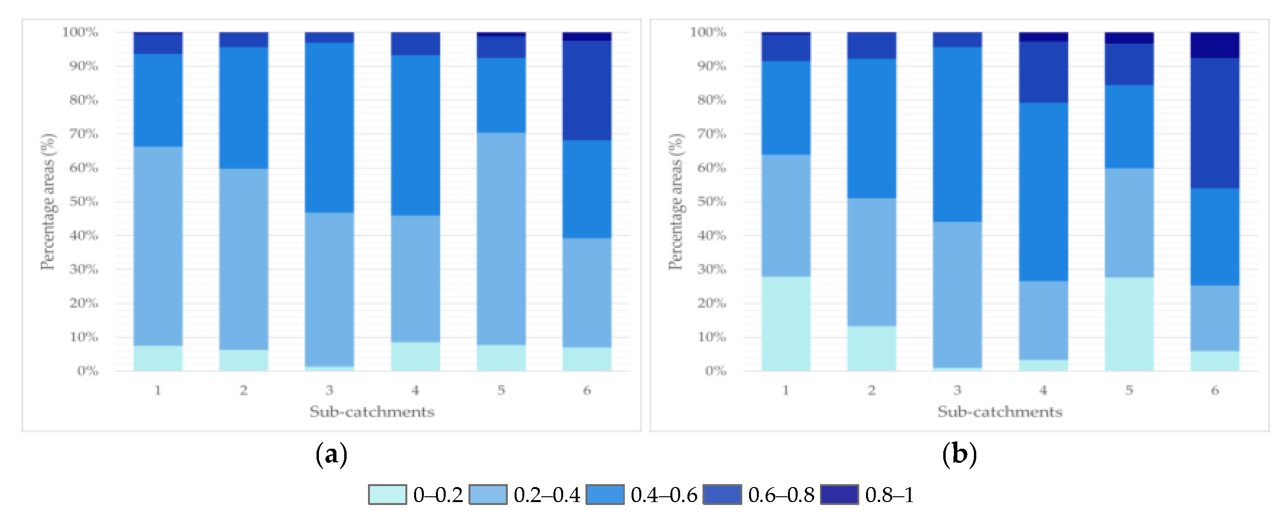
Areas with higher LCI values in 1997 (Figure 8a) were present in the greatest proportion in sub-catchment 6 (30%), 5 (9%) and 4 (7%), while areas with lowest LCI values dominated in sub-catchment 3 (54%). In 2017 (Figure 8b), areas with higher LCI values increased in sub-catchments 6, 5 and 4 to occupy 47%, 16% and 32%, respectively, while areas with the lowest LCI values still dominated in sub-catchment 3 (54%). Compared with 1997, in 2017 all six sub-catchments showed increases in areas with higher LCI values, and corresponding decreases mainly in the dominant LCI class 0.2–0.4.
3.2. Runoff Indicator (RoI)
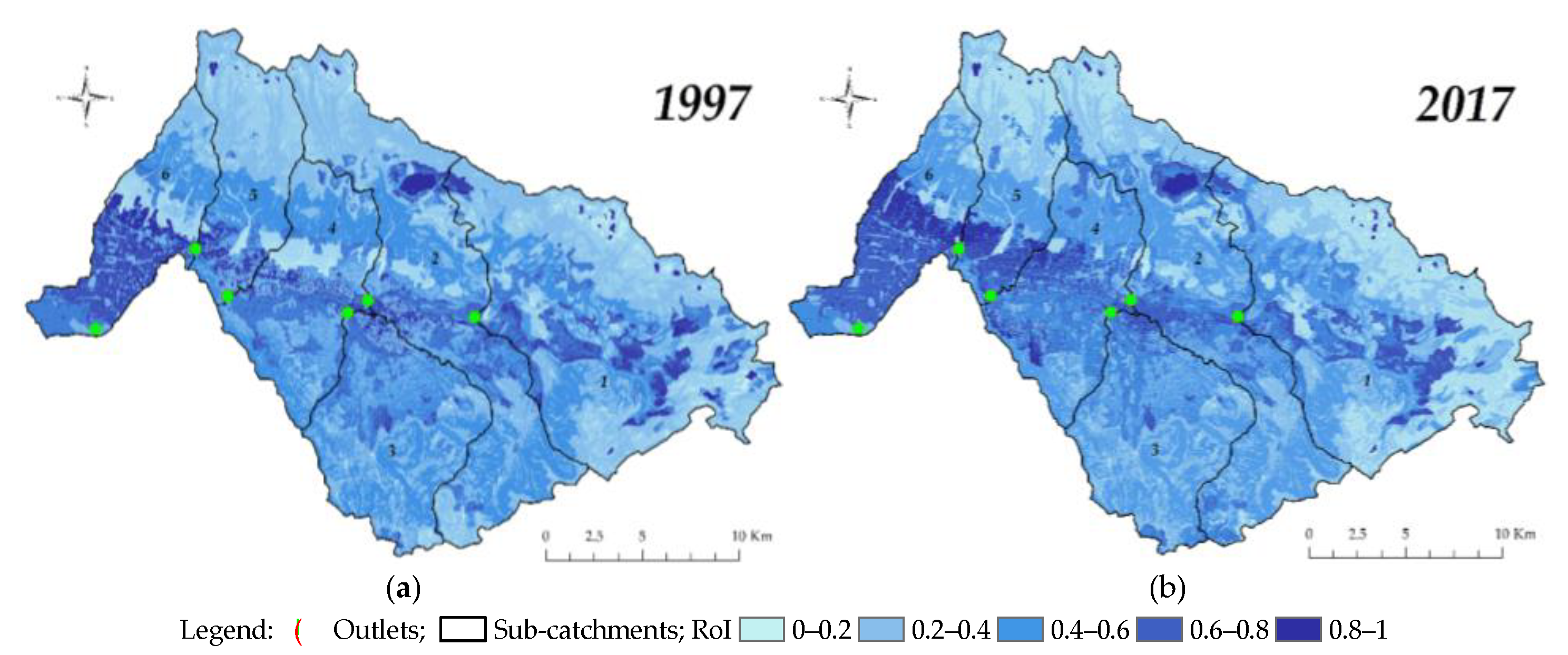
The distribution of RoI in 1997 and 2017 is presented in Figure 9. Higher RoI values (0.6–0.8; 0.8–1, see Table 2) corresponded to the interactions of impervious or hard surfaces, mostly related to human settlements with higher percentage area with impervious surface, with slope >10% and with clay and silt soil texture (low water permeability). At the other end of the scale, low RoI values (RoI 0–0.2; 0.2–0.4) were related mostly to forest/shrubland, grassland (semi-natural vegetation cover) and cropland, interacting with >45% sand soil texture (high water permeability rates) and slope <5%. Medium RoI values (RoI 0.4–0.6) were related to the interaction between cropland, clay and silt soil texture and 5–10% slope.
In 1997, areas with higher RoI values (Figure 9a) covered approximately 11% of the total catchment area, while lower RoI values covered approximately 55%. In 2017, areas with higher RoI values (Figure 9b) increased to cover approximately 17% of the catchment area, while lower RoI values covered approximately 46%. The study catchment was dominated by RoI classes 0.2–0.4 and 0.4–0.6 in 1997 (49% and 34%, respectively) and in 2017 (31% and 37%, respectively).
In 1997, areas with higher RoI values were present in the greatest proportions in sub-catchment 6 (32%), while areas with lower RoI values were present in the greatest proportions in sub-catchments 5 (70%), 1 (66%) and 2 (60%) (Figure 10a). In 2017, areas with higher RoI values increased in sub-catchments 6, 4 and 5, to 46%, 21% and 16%, respectively, while areas with lower RoI values decreased in sub-catchments 1, 5 and 2, to 64%, 60% and 51%, respectively (Figure 10b). The study sub-catchments were dominated by RoI classes 0.2–0.4 and 0.4–0.6 in both 1997 and 2017. In general, in 2017 compared with 1997, sub-catchments showed increases in higher RoI values, but also decreases in lower RoI values and in the dominant LCI 0.2–0.4 class.
3.3. Distance Indicator (DI)
The distribution of DI classes in the catchment is shown in Figure 11, where red indicates short distances and green longer distances. The highest DI values (DI 0.8–1) corresponded to areas with numerous river network tributaries (i.e., close proximity to the river network; see also Figure 2a) located on steep slopes, while the lowest DI values (DI 0–0.2) were related to few river tributaries on gentle slopes.
3.4. Potential Non-Point Pollution
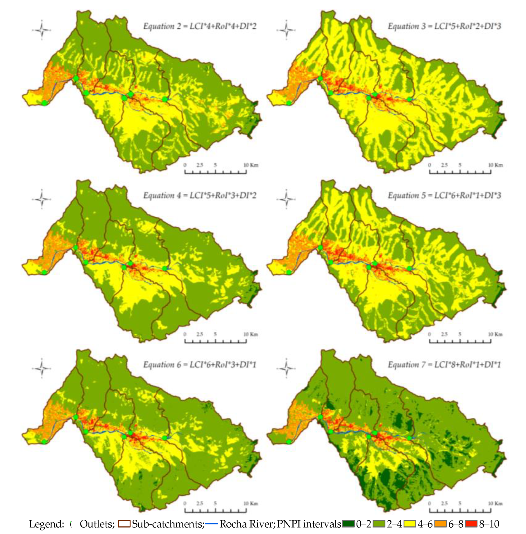
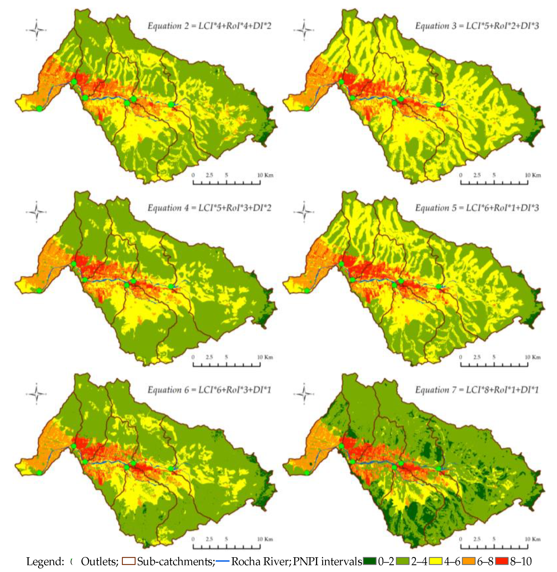
The distribution of PNPI classes, resulting from Equations (2)–(7), are presented in Figure 12 for 1997 and in Figure 13 for 2017.
Areas with higher PNPI values (6–8; 8–10, see Table 4) were mainly concentrated along the middle section in the valley lowlands, around the Rocha River main channel (Figure 12 and Figure 13). These areas have higher potential for generation of non-point pollution due to human settlements (Figure 4) with higher population densities (>120 persons per ha) and higher LCI values (Figure 7), higher pollutant mobility due to higher RoI values (Figure 9) and higher DI values (shorter distances to river network; <520 m) (Figure 11). Human settlements in Sacaba and Cochabamba cities, which have increased from 1997 to 2017, were located in these areas. Areas with lower pollution potential (PNPI classes 0–2, 2–4) surrounded the central part towards the edges of the catchment (but not the western part). They corresponded to lower potential generation of non-point pollution due to semi-natural related land use types (forest, shrubland, grassland and mountain lakes) and thus lower LCI values, and low pollutant mobility due to lower RoI and DI (distances to river network >1704 m).
The area occupied by the different PNPI classes shown in Figure 12 and Figure 13 is presented in Table 6. In general, increases between 1997 and 2017 in areas covered by higher PNPI classes occurred in increasing order from sub-catchments 1 to 6, while decreases in lower PNPI classes were found for all sub-catchments (Equations (2)–(7)). The area resulting from Equation (6) increased (19%; PNPI 4–6) and decreased (27%; PNPI 2–4) most between 1997 and 2017, while the PNPI class 4–6 (yellow in Figure 12 and Figure 13) varied the most for all six sub-catchments (Equations (2)–(7)). Area with the lowest PNPI class (0–2) remained the same in both time periods, with no significant changes (maximum 1%).
The higher relative importance of LCI was reflected in Equations (5)–(7), where higher weighting values were assigned to LCI. High relative importance of RoI in comparison with DI was reflected in Equations (2), (4) and (6). The effect of DI, as a result of Equations (3) and (5) where DI was weighted with higher values than RoI, was visible as closest distances to river network, i.e., yellow representing the stream network. In both 1997 and 2017, Equations (3) and (5) gave a higher proportion of PNPI class 4–6 (yellow) land, while Equation (7) gave a higher proportion of PNPI class 0–4 land (greenish). Equations (2), (4) and (6) were relatively similar to each other, and intermediate between the two extremes of Equations (3) and (7).
On analysing sub-catchments, mean PNPI values showed clear increases in 2017 compared with 1997 (Table 7). The highest increases were for Equation (6) (lowest relative importance for DI and higher importance for LCI) and the lowest increases were for Equation (3) (DI slightly more important than RoI, LCI having lower relative importance than for Equation (6). Mean PNPI values showed a general trend to increase from sub-catchment 1 to 6, with the exception of a decrease in sub-catchment 5. For instance, Equation (6) in 1997 gave mean PNPI values of 3.0, 3.3, 3.4, 3.8, 3.4 and 4.5 for sub-catchments 1, 2, 3, 4, 5 and 6, respectively, while the corresponding mean PNPI values in 2017 were 3.8, 4.4, 4.4, 5.6, 4.8 and 5.8, respectively. Finally, sub-catchments 4, 5 and 6 showed a greater increase in mean PNPI compared with sub-catchments 1, 2 and 3 for all equations in both years.
The accumulated mean PNPI values due to water flow from upstream sub-catchments to the respective downstream sub-catchments are presented in Table 8. They showed increases in 2017 compared with 1997 and a general trend for an increase from sub-catchment 1 to 6, with the exception of a decrease in sub-catchments 4 and 5. Sub-catchments 4, 5 and 6 showed higher PNPI values than sub-catchments 1, 2 and 3 for all equations in both years.
Measured mean nitrate (NO3) and phosphate (PO4) concentrations at the outlets of the sub-catchments in 1997 and 2017 [21] are presented in Table 9. Both NO3 and PO4 concentrations increased from 1997 to 2017, except for a decrease in NO3 in sub-catchment 6 in 2017. A clear increase in PO4 concentration was observed in sub-catchments 3, 5 and 6 in 2017.
Correlation analysis revealed significant relationships between PO4 and PNPI values obtained with all equations in 2017, indicating that PO4 increased with increasing PNPI (Table 10). No other relationships were significant, but all correlation coefficients were positive, showing a trend for increasing NO3/PO4 values with increasing PNPI.
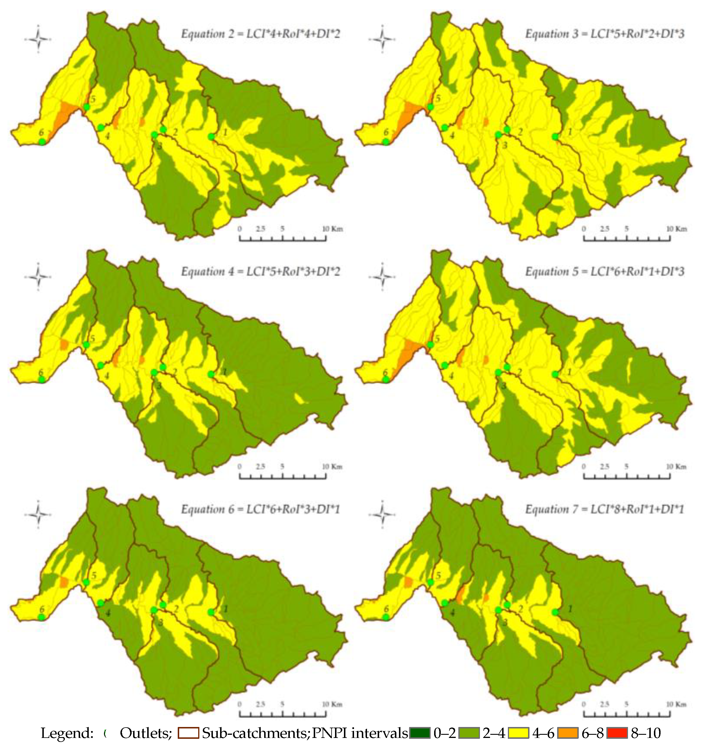
The PNPI results for the catchment (Figure 12 and Figure 13) were aggregated into micro-catchments (Figure 14 and Figure 15) to identify priority source areas (PSAs), as decision support for recommendations on appropriate management measures to reduce pollution potential in different parts of the catchment.
In 1997, PSAs with the highest and lowest pollution potential (PNPI classes 8–10 and 0–2, respectively; see Table 4) were not present at all in the catchment. Medium-high potential pollution (PNPI class 6–8) was rarely present (Figure 14), representing less than 3% of the total catchment area (between 0.3% with Equation (6) and 2% with Equation (5)). As a consequence, areas of low-medium potential pollution (PNPI class 2–4) (which covered 80% with Equation (7)) and medium potential pollution (PNPI 4–6) (which covered 75% with Equation (3)), dominated the catchment in different proportions depending on the equation used.
Areas of medium-high PNPI were present in the greatest proportions in the catchment with Equations (2), (3) and (5). With Equation (5), they covered 15% of sub-catchment 6, 3% of sub-catchment 4 and 0.2% of sub-catchments 3 and 2, while they were not present in sub-catchments 1 and 5. Equation (5) results for the other sub-catchments confirmed the dominance of areas with medium PNPI (95% in sub-catchment 4) and low-medium PNPI (68% in sub-catchment 1).
In 2017, PSAs showing the highest pollution potential (PNPI class 8–10; see Table 4) appeared only in the case of Equation (5), covering 0.3% of the total catchment (Figure 15). In relation to 1997 (Figure 14), areas corresponding to medium-high pollution potential (PNPI 6–8) clearly increased for all equations, to up to 15% with Equation (3). Conversely, areas of medium pollution potential (PNPI class 4–6) decreased from 1997 to 2017 for all equations (e.g., from 75% in 1997 to 62% in 2017 with Equation (3)), as did areas with low-medium pollution potential (PNPI class 2–4) (e.g., from 80% in 1997 to 73% in 2017 with Equation (3)). However, these two classes still dominated the entire catchment for all equations. As in 1997, area with the lowest pollution potential (PNPI class 0–2) was not present in the catchment in 2017.
At sub-catchment level, Equation (5) gave the highest PNPI in 2.1% of the area in sub-catchment 4, while areas of medium-high PNPI represented 58%, 41% and 24% of sub-catchments 6, 5 and 4, respectively. Equation (5) confirmed the dominance of medium PNPI (55%) in sub-catchment 4 and low-medium PNPI (64%) in sub-catchment 1.
4. Discussion
4.1. Relative Importance of Indicators
Rapid and inappropriate urbanisation in the study area was reflected in a PNPI increase in 2017 compared with 1997. Migration from the countryside and economic activities have increased the pollution pressure, through development without proper waste management, a deficient water supply and inadequate sanitation services.
In the present study, eight general land use types were identified and used in the analysis, which is fewer than in previous studies [18,19,20]. These eight were selected from the CORINE (Coordination of Information on the Environment) land cover classification system [54], which includes 44 types. Similar numbers of land use types as in the present study (between four and six) have been used in some previous studies [11,37,55]. In those studies, land use classification integrated contextual information related to pollution potential (e.g., fertiliser inputs, pollutant or nutrient load and export) for each land use type and its management, in addition to the land use classification.
Land use type weighting to obtain LCI (see Table 1), as used in the present study, combines widely available data and is relatively simple to calculate and work with on a GIS interface. It also gives direct reference to the driving forces of pollution, by taking N and P (applied as manure or chemical fertiliser) as the main indicators. These are the most widely studied indicators directly related to NPSP [15,56]. However, difficulties arise in (1) defining a proper land use label regarding the purpose of the study (number and properties); (2) related land use with pollution loads as pollutant source; (3) sewage characterisation, since it is deficient or absent in data-scarce areas; and (4) possible effects of runoff retention or increased runoff rate in each particular land use type. Thus, an optimum LCI definition should be addressed by an adequate weighting of land use types in terms of the most representative pollutant in runoff and how they are associated.
In the PNPI assessment, the most important indicator was confirmed to be LCI, because of potential pollution generation and high relative importance weighted in Equations (1)–(6). The main reason for this were that the city of Sacaba lacks an efficient sewerage system and water treatment plants, and the city of Cochabamba treats only a small proportion of the sewage generated [34]. More detailed studies are needed on pollution related to cropland and its management, and on the effects of grassland in pollution control, in the study catchment [57]. An association between urban areas (human settlements) and higher LCI values has been found in previous land use/land cover evaluations [18,19,20], using similar indices to PNPI, such as agricultural nonpoint pollution potential index (APPI) [15,58] and multicriteria analysis [11,13,55]. On a medium working scale (covering the study catchment) of 1:50.000 spatial resolution to match Landsat imagery pixels and SRTM-DEM resolution (30 m × 30 m), the land use and LCI results (and later PNPI) showed agreement. Upscaling of the land use information did not substantially affect the results, as previously reported for NPSP modelling and water runoff and sediment yield assessment [15,59,60].
Land use types showed changes (increases/decreases) between 1997 and 2017 (e.g., human settlements increased), which influenced the RoI results obtained (Figure 9 and Figure 10). The impervious or hard surfaces that dominate human settlements are known to have a significant influence in runoff generation, even during the small rainstorm events that are frequent in the rainy season in Bolivia [61,62].
Runoff coefficient (Ci) was determined through GIS and remote sensing, an approach that is widely accepted in hydrology and water resources management when dealing with data-scarce regions [61,63,64] or in large-scale rapid analyses [65]. The movement of nutrients or pollutants from land surface to Rocha River stream network is controlled by surface runoff due to topography, soil characteristics and rainfall pattern. High runoff rates most likely increase the mobility of sediments and associated pollutants.
A more precise approach to calculating runoff and other hydrological parameters would require field data (rain and flow) for calibration and validation of predicted results. Learning from similar gauged catchment areas in the region may lead to adequate results, but information later than 2014 was not available for the present study.
In the study catchment, the main source of recharge for river flow is precipitation, but illegal domestic sewage water and small industrial spills to the river act as additional sources and can be considered the only inputs during dry periods. Higher amounts of precipitation in the rainy season can contribute to increased surface runoff and pollutant wash-off from adjacent areas to the main river. According to the literature, river water quality in regions with a similar climate to the study area is low in the dry season, as a consequence of low river flow, while in the rainy season higher water flow dilutes the pollutant concentrations [5,14]. Nitrate and phosphate concentrations in the dry season were used to validate the PNPI results, but more extensive research is needed to determine the effect of precipitation variation (yearly, seasonally, monthly) on the approach used here.
Modelling of DI reflected the fact that about 70% of the study catchment consisted of mountainous region and 30% of fluvial plains. A previous study in a region with fewer mountainous areas (33%) and more fluvial plains (67%) also found high DI values for a dense stream network along major river tributaries [11]. Thus high DI values mainly depend on the density of the river stream network (large number of tributaries) and high runoff in mountainous topography. The approach of assigning higher DI values for shorter distances to the river network, and lower DI values for longer distances, has been used previously [18,19,20,66].
Possible changes in the Rocha River stream network due to new human settlements and to drainage channels and ditches to prevent flooding in the rainy season were not considered in the present analysis, since no accurate available information was found. Local landscape patterns and rainstorm-driven events in part of the year can be considered to reduce non-point pollution by capturing runoff in some areas [66]. Wetland areas can act as sinks and/or sources of sediments and pollutants in surface runoff, allowing these to settle and become trapped and later remobilised [9,31,67].
4.2. Potential Non-Point Pollution Index (PNPI)
In this study, the results of indicator weightings for PNPI were integrated using the weighted sum tool in ArcGIS 10.7. Previous studies with PNPI have used simple map algebra integration of the three independent indicators (land cover, runoff and distance to river) in ArcView GIS ver. 3.2 [18,19,20,44]. Our approach can be considered an improvement and process optimisation in computational analysis, since it uses technological advances in PNSP analysis. Weights differed in Equation (2) to Equation (7) based on relative importance of indicators in generation of potential pollution, but LCI was identified as the most important indicator in all equations. In a previous study using this approach, the LCI and RoI weighting values were changed to make these the most important factors (DI was not considered due to short distances in the study area) [37]. A widely accepted multi-attribute decision-making approach for weighting, technique for order preference by similarity to ideal solution (TOPSIS) [68], has been found to be helpful because it can reduce subjectivity errors by assuming a monotonic increase or decrease in attributes in a decision matrix [11,55]. A disadvantage of the rank sum method used in the present study is the lack of theoretical foundation and the difficulty in justifying the assigned weights, and therefore sensitivity analysis becomes particularly difficult.
The GIS modelling results for PNPI showed that the lacking or ineffective sewage systems in human settlements in the study catchment can be considered the main contributing factor to potential pollution generation. Solid waste generation and inadequate disposal, soil erosion and surface runoff in sensitive areas (waste disposal sites, septic system failures and construction sites) were also shown to be important contributing factors. An association between high PNPI values and urbanisation has been reported previously [18,19,20], with higher PNPI values for intensely populated (human settlements) or cultivated areas in all major cities, steep slopes and short distance to the river network. In contrast, a study in Sweden by Wesström and Joel [37] found that urban areas were associated with lower PNPI values, since all water discharges are properly treated in Sweden, and that higher PNPI values were related to intense cropping systems such as potatoes and close to mink farms.
In the literature, high PNPI values are generally related to heavy fertilisation in agriculture, but fertilisation rates in Bolivian agriculture are usually low and the main fertiliser used is manure. Due to the cost, additional chemical fertiliser is seldom used except for crops of economic importance, like some vegetables and greens (onions, tomatoes, carrots, lettuce, radish among others), potatoes and maize. Thus APPI may be an inadequate index for use in the study catchment, since most of the pollution potential is from human settlements. APPI has been used to identify a relationship between densely populated areas, high anthropogenic activities and high pollution potential [11,55].
The nitrate and phosphate concentrations (used for validation) within sub-catchments in the study area increased during the study period (Table 9). This was possibly due to: (1) sewage water discharge from human settlements which include houses, industries and other economic activities; (2) runoff from fertilised land, which increased in the period (see Figure 9 and Figure 10); and (3) soil erosion runoff. Sampling-related events can also have affected the nitrate and phosphate concentrations, since sample numbers were limited and the weather can be variable in the dry season, when sampling was carried out. Validation results revealed a significant relationship (Pearson correlation) between PNPI and phosphate only in 2017 and only a trend for an increase between PNPI and nitrate (Table 10). Better stability and higher concentrations of phosphate compared with nitrate in water samples can explain this correlation, since nitrate can easily be transformed into other nitrogenous compounds under the influence of temperature (water and environment), solar radiation and other chemicals present. A similar clear positive relationship was found in a previous study, where low water quality status was compared against nitrogen loss potential from NPSP [11]. The validation results could be improved by collecting samples in different periods of the year, to better represent the effects of hydrological regime. Munafò et al. [18] proposed validation of PNPI results by comparison against output from a physical based model. However, the use of physical models can increase the data requirement (collection, quality evaluation, time and technical skills), hampering use of PNPI for identification of PSAs using multi-criteria analysis and GIS implementation and representation in data-scarce regions.
The advantage of identifying PSAs by PNPI lies in the indicators providing a proper representation of landscape features (land use, runoff and distant to stream network) at multiple levels (catchment, sub-catchment, micro-catchment). PNPI can be calculated for data-scarce regions and is a simple, effective and less time- and resource-demanding approach. Limitations with PNPI are lack of available information on indicators and uncertainty in observed nitrate and phosphate concentrations used for validation, in this study. Future studies should examine how landscape features and detailed hydrological, chemical and geographical processes interact in PSA prediction with scarce data.
The results presented here for the sub-catchment scale provide an overview of the NSPS situation in the catchment. For management purposes, the results obtained at micro-catchment scale can be useful for identifying priority intervention areas.
5. Conclusions
A multi-criteria approach including analyses at various scales and GIS-based PNPI modelling, which combined weighted sum of indicators, was used to identify and rank priority source areas (hotspot areas) that are more likely to produce pollution within micro-catchments and sub-catchments in the Rocha River catchment, Bolivia.
Increased area of human settlements in 2017 compared with 1997 (22% and 14%, respectively) and decreased area of semi-natural land use types resulted in higher PNPI values in many areas, identifying them as PSAs where recommended management practices should be improved.
The PNPI results indicated that PSAs in the study catchment are mainly associated with densely populated human settlements and that agricultural areas play a minor role in NPSP generation, since crop fertilisation is based predominantly on manure.
The PNPI model can thus be a useful tool for environmental management, policy decision-making and to inform public opinion. The methodological approach described may be applicable to other watersheds in Bolivia and elsewhere with similar landscape characteristics and hydrological features. It may be particularly useful in data-poor regions in developing countries where NPSP knowledge needs to be improved.
Author Contributions
Conceptualization, A.J., I.W. and B.G.; methodology, B.G., I.W., I.M. and A.J.; software, B.G. and A.J.; validation, I.W., I.M. and A.J; formal analysis, B.G., I.W., I.M. and A.J.; investigation, B.G. and M.V.; writing—review and editing, B.G., I.W., I.M. and A.J; supervision, I.W., I.M., M.V. and A.J. All authors have read and agreed to the published version of the manuscript.
Funding
This research was funded by the Swedish International Development Cooperation Agency (SIDA), Sida contribution number 75000554 and 75000554-09.
Acknowledgments
The authors would like to acknowledge the staff at San Simon University (UMSS) for providing logistic support for this project. We also want to thank Mary McAfee for valuable inputs and English corrections.
Conflicts of Interest
The authors declare no conflict of interest. The funders had no role in the design of the study; in the collection, analyses, or interpretation of data; in the writing of the manuscript, or in the decision to publish the results.
References
- Chen, X.; Zhou, W.; Pickett, S.T.; Li, W.; Han, L. Spatial-Temporal Variations of Water Quality and Its Relationship to Land Use and Land Cover in Beijing, China. Int. J. Environ. Res. Public Health 2016, 13, 449. [Google Scholar] [CrossRef] [PubMed] [Green Version]
- Schaffner, M.; Bader, H.-P.; Scheidegger, R. Modeling the contribution of point sources and non-point sources to Thachin River water pollution. Sci. Total. Environ. 2009, 407, 4902–4915. [Google Scholar] [CrossRef]
- Novotny, V. Water Quality: Diffuse Pollution and Watershed Management; The Royal Geographical Society (with the Institute of British Geographers): London, UK, 2002. [Google Scholar]
- Mi, Y.; He, C.; Bian, H.; Cai, Y.; Sheng, L.; Ma, L. Ecological engineering restoration of a non-point source polluted river in Northern China. Ecol. Eng. 2015, 76, 142–150. [Google Scholar] [CrossRef]
- Zhu, Q.D.H.; Sun, J.H.; Hua, G.F.; Wang, J.H.; Wang, H. Runoff characteristics and non-point source pollution analysis in the Taihu Lake Basin: A case study of the town of Xueyan, China. Environ. Sci. Pollut. Res. 2015, 22, 15029–15036. [Google Scholar] [CrossRef] [PubMed]
- Corwin, D.L.; Loague, K.; Ellsworth, T.R. Introduction: Assessing non-point source pollution in the vadose zone with advanced information technologies. Hydrogeol. Chem. Weather. Soil Form. 1999, 108, 1–20. [Google Scholar] [CrossRef]
- Loague, K.; Corwin, D.L.; Ellsworth, A.T.R. Feature: The Challenge of Predicting Nonpoint Source Pollution. Environ. Sci. Technol. 1998, 32, 130A–133A. [Google Scholar] [CrossRef]
- Giri, S.; Qiu, Z. Understanding the relationship of land uses and water quality in Twenty First Century: A review. J. Environ. Manag. 2016, 173, 41–48. [Google Scholar] [CrossRef] [Green Version]
- Wang, J.; Shao, J.; Wang, D.; Ni, J.; Xie, D. Identification of the “source” and “sink” patterns influencing non-point source pollution in the Three Gorges Reservoir Area. J. Geogr. Sci. 2016, 26, 1431–1448. [Google Scholar] [CrossRef]
- Zhang, J. Discussion on Non-point Source Pollution and Control in Water Source Areas. In Study of Ecological Engineering of Human Settlements; Springer Nature: Berlin/Heidelberg, Germany, 2019; pp. 197–221. [Google Scholar]
- Zhang, H.; Huang, G. Assessment of non-point source pollution using a spatial multicriteria analysis approach. Ecol. Model. 2011, 222, 313–321. [Google Scholar] [CrossRef]
- Maillard, P.; Pineheiro Santos, N.A. A spatial statistical approach for modeling the effect of non-point source pollution on different water quality parameters in the Velhas River watershed–Brazil. J. Environ. Manag. 2008, 86, 158. [Google Scholar] [CrossRef] [PubMed]
- Li, K.-C.; Yeh, M. Nonpoint source pollution potential index: A case study of the Feitsui Reservoir watershed, Taiwan. J. Chin. Inst. Eng. 2004, 27, 253–259. [Google Scholar] [CrossRef]
- De Oliveira, L.M.; Maillard, P.; Pinto, E.J.D.A. Application of a land cover pollution index to model non-point pollution sources in a Brazilian watershed. Catena 2017, 150, 124–132. [Google Scholar] [CrossRef]
- Shen, Z.; Hong, Q.; Chu, Z.; Gong, Y. A framework for priority non-point source area identification and load estimation integrated with APPI and PLOAD model in Fujiang Watershed, China. Agric. Water Manag. 2011, 98, 977–989. [Google Scholar] [CrossRef]
- Kliment, Z.; Kadlec, J.; Langhammer, J. Evaluation of suspended load changes using AnnAGNPS and SWAT semi-empirical erosion models. Catena 2008, 73, 286–299. [Google Scholar] [CrossRef]
- Heathwaite, L.; Sharpley, A.N.; Gburek, W. A Conceptual Approach for Integrating Phosphorus and Nitrogen Management at Watershed Scales. J. Environ. Qual. 2000, 29, 158–166. [Google Scholar] [CrossRef]
- Munafò, M.; Cecchi, G.; Baiocco, F.; Mancini, L. River pollution from non-point sources: A new simplified method of assessment. J. Environ. Manag. 2005, 77, 93–98. [Google Scholar] [CrossRef]
- Cecchi, G.; Munafò, M.; Baiocco, F.; Andreani, P.; Mancini, L. Estimating river pollution from diffuse sources in the Viterbo province using the potential non-point pollution index. Annali dell’Istituto Superiore di Sanità 2007, 43, 295–301. [Google Scholar] [PubMed]
- Ciambella, M.; Venanzi, D.; Dello, E.; Andreani, P.; Cecchi, G.; Formichetti, P.; Munafò, M.; Mancini, L. Convenzione Istituto Superiore Di Sanità-Provincia Di Viterbo: Messa a punto di uno strumento conoscitivo per la gestione delle acque superficiali della Provincia di Viterbo; Convenzione Istituto Superiore Di Sanità-Provincia Di Viterbo: Viterbo, Italy, 2005; pp. 227–238. [Google Scholar]
- CGE (Contraloria General del Estado). Informe de Auditoría Sobre el Desempeño Ambiental Respecto de los Impactos Negativos Generados en el Río Rocha (Audit Report about Environmental Performance Regarding Negative Impacts Generated on the Rocha River); K2/AP06/M11; Gestión de Evaluación Ambiental: Cochabamba, Bolivia, 2011; p. 320. [Google Scholar]
- PDC (Prefectura del Departamento de Cochabamba). Estudios Básicos de la Cuenca del Río Rocha (Rocha River Watershed Basic Studies); Dirección departamental de Recursos Naturales–DDRN: Cochabamba, Bolivia, 2005; p. 314. [Google Scholar]
- Romero, A.; Van Damme, P.; Goitia, E. Contaminación orgánica en el río Rocha (Cochabamba, Bolivia) (Organic contamination of the Rocha river (Cochabamba, Bolivia)). Rev. Boliv. Ecol. Conserv. Ambient. 1998, 8, 37–47. [Google Scholar]
- Gossweiler, B.; Wesström, I.; Messing, I.; Romero, A.M.; Joel, A. Spatial and Temporal Variations in Water Quality and Land Use in a Semi-Arid Catchment in Bolivia. Water 2019, 11, 2227. [Google Scholar] [CrossRef] [Green Version]
- Metternicht, G.; Gonzalez, S. FUERO: Foundations of a fuzzy exploratory model for soil erosion hazard prediction. Environ. Model. Softw. 2005, 20, 715–728. [Google Scholar] [CrossRef]
- Metternicht, G.; Fermont, A. Estimating Erosion Surface Features by Linear Mixture Modeling. Remote Sens. Environ. 1998, 64, 254–265. [Google Scholar] [CrossRef]
- Holdridge, L.R. Determination of World Plant Formations From Simple Climatic Data. Science 1947, 105, 367–368. [Google Scholar] [CrossRef]
- Ongaro, L. Land Evaluation of the Valley of Sacaba (Bolivia). In Remote Sensing and Natural Resources Evaluation; Istituto agronomico per l’oltremare, Ed.; Ministero degli affari esteri: Firenze, Italy, 1998; p. 177. [Google Scholar]
- MMAA (Ministerio de Medio Ambiente y Agua de Bolivia). Sistematización Sobre Tratamiento y Reúso de Aguas Residuales (Wastewater Treatment and Reuse Systematization on); Programa de Desarrollo Agropecuario Sustentable—Proagro: La Paz, Bolivia, 2013. [Google Scholar]
- INE (Instituto Nacional de Estadística). Censo Nacional de Población y Vivienda 2012. In Crecimiento Intercensal por Municipios (National Population and Housing Census 2012, Intercensal Growth by Municipalities); Estado Plutrinacional de Bolivia: La Paz, Bolivia, 2013; p. 56. [Google Scholar]
- UN-GEOBOL (United Nations-Servicio Geologico de Bolivia). Investigaciones de Aguas Subterráneas en las Cuencas de Cochabamba (Study of the Groundwaters of Basins of the Cochabamba Department). In Informe Técnico (Technical Report) 1; Proyecto Integrado de Recursos Hidricos (PIRHC): Cochabamba, Bolivia, 1978. [Google Scholar]
- Stimson, J.; Frape, S.; Drimmie, R.; Rudolph, D. Isotopic and geochemical evidence of regional-scale anisotropy and interconnectivity of an alluvial fan system, Cochabamba Valley, Bolivia. Appl. Geochem. 2001, 16, 1097–1114. [Google Scholar] [CrossRef]
- Renner, S.; Velasco, C. Geology and Hydrogeology of the Central Valley of Cochabamba; Geology and Minning National Service: La Paz, Bolivia, 2000; Volume 34, p. 125. [Google Scholar]
- Trohanis, Z.; Zaengerling, B.; Sanchez-Reaza, J. Urbanization trends in Bolivia. In Opportunities and Challenges; The World Bank: Washington, DC, USA, 2015. [Google Scholar]
- MMAA (Ministerio de Medio Ambiente y Agua de Bolivia). Inventario de Principales Fuentes de Contaminación en la Cuenca del Rio Rocha (Municipios de Sacaba, Cochabamba, Colcapirhua, Quillacollo, Vinto y Sipe Sipe) (Inventory of Main Pollution Sources in the Rocha River Watershed (Municipalities of Sacaba, Cochabamba, Colcapirhua, Quillacollo, Vinto and Sipe Sipe)); Viceministerio de Recursos Hídricos y Riego–VRHR: La Paz, Bolivia, 2017. [Google Scholar]
- Maathuis, B.H.P.; Wang, L. Digital Elevation Model Based Hydro-processing. Geocarto Int. 2006, 21, 21–26. [Google Scholar] [CrossRef]
- Wesström, I.; Joel, A. In Storage and reuse of drainage water. In Proceedings of the 9th International Drainage Symposium held jointly with CIGR and CSBE/SCGAB, Quebec City, QC, Canada, 13–16 June 2010; American Society of Agricultural and Biological Engineers: St. Joseph, MI, USA, 2010; p. 10. [Google Scholar] [CrossRef]
- GAMS (Gobierno Autónomo Municipal de Sacaba). Plan Territorial de Desarrollo Integral—PTDT (Integral Development Territorial Plan—IDTP); Secretaria Municipal de Planificación y Desarrollo Territorial: Sacaba, Cochabamba, Bolivia, 2016; p. 294. [Google Scholar]
- Aguilera, X.; Declerck, S.A.J.; De Meester, L.; Maldonado, M.; Ollevier, F. Tropical high Andes lakes: A limnological survey and an assessment of exotic rainbow trout (Oncorhynchus mykiss). Limnologica 2006, 36, 258–268. [Google Scholar] [CrossRef] [Green Version]
- Jacobs, S.R.; Weeser, B.; Guzha, A.C.; Rufino, M.C.; Butterbach-Bahl, K.; Windhorst, D.; Breuer, L. Using High-Resolution Data to Assess Land Use Impact on Nitrate Dynamics in East African Tropical Montane Catchments. Water Resour. Res. 2018, 54, 1812–1830. [Google Scholar] [CrossRef] [Green Version]
- Smith, V.; Swaney, P.; Talaue-Mcmanus, L.; Bartley, D.; Sandhei, T.; McLaughlin, J.; Dupra, C.; Crossland, J.; Buddemeier, W.; Maxwell, A.; et al. Humans, Hydrology, and the Distribution of Inorganic Nutrient Loading to the Ocean. Bioscience 2003, 53, 235–245. [Google Scholar] [CrossRef]
- Santos, I.R.; Costa, R.C.; Freitas, U.; Fillmann, G. Influence of effluents from a Wastewater Treatment Plant on nutrient distribution in a coastal creek from southern Brazil. Braz. Arch. Biol. Technol. 2008, 51, 153–162. [Google Scholar] [CrossRef] [Green Version]
- Van Drecht, G.; Bouwman, A.F.; Harrison, J.; Knoop, J.M. Global nitrogen and phosphate in urban wastewater for the period 1970 to 2050. Glob. Biogeochem. Cycles 2009, 23, 4. [Google Scholar] [CrossRef] [Green Version]
- Puccinelli, C.; Marcheggiani, S.; Munafò, M.; Andreani, P.; Mancini, L. Evaluation of Aquatic Ecosystem Health Using the Potential Non Point Pollution Index (PNPI) Tool. In Diversity of Ecosystems; Ali, M., Ed.; InTech: London, UK, 2012; p. 16. ISBN 978-953-51-0572-5. [Google Scholar]
- Goel, M. Runoff Coefficient. In Encyclopedia of Snow, Ice and Glaciers; Singh, V.P., Singh, P., Haritashya, U.K., Eds.; Springer: Berlin/Heidelberg, Germany, 2011; pp. 952–953. [Google Scholar]
- The Clean Water Team Runoff Coefficient, FS-5.1.3. (RC), SWAMP—Clean Water Team Citizen Monitoring Program, Guidance Compendium for Watershed Monitoring and Assessment. Available online: https://www.waterboards.ca.gov/water_issues/programs/swamp/docs/cwt/guidance/513.pdf (accessed on 21 November 2019).
- Schwab, G.; Frevert, R.; Edminster, T.; Barnes, K. Soil and Water Conservation Engineering; John Wiley and Sons: New York, NY, USA, 1981. [Google Scholar]
- Hudson, N. Field Measurement of Soil Erosion and Runoff; Food & Agriculture Orgriculture—FAO: Rome, Italy, 1993; Volume 68. [Google Scholar]
- Zinck, J.; Metternicht, G.; Bocco, G.; Del Valle, H. Geopedology Elements of Geomorphology for Soil and Geohazard Studies; ITC Special Lecture Notes Series: Enschede, The Netherlands, 2013. [Google Scholar]
- Metternicht, G. Detecting and Monitoring Land Degradation Features and Processes in the Cochabamba Valleys, Bolivia: A Synergistic Approach. Ph.D. Thesis, University of Ghent, Enschede, The Netherlands, 1996. [Google Scholar]
- Jenks, G. The data model concept in statistical mapping. Int. Yearb. Cartogr. 1967, 7, 186–190. [Google Scholar]
- Arora, J. Multi-objective Optimum Design Concepts and Methods. In Introduction to Optimum Design, 3rd ed.; Arora, J.S., Ed.; Academic Press: Boston, MA, USA, 2012; pp. 657–679. [Google Scholar]
- Stillwell, W.G.; Seaver, D.A.; Edwards, W. A comparison of weight approximation techniques in multiattribute utility decision making. Organ. Behav. Hum. Perform. 1981, 28, 62–77. [Google Scholar] [CrossRef]
- Bossard, M.; Feranec, J.; Otahel, J. CORINE Land Cover Technical Guide: Addendum; EEA (European Environment Agency): Copenhagen, Denmark, 2000; p. 105. [Google Scholar]
- Wu, B.; Zhang, X.; Xu, J.; Liu, J.; Wei, F. Assessment and management of nonpoint source pollution based on multicriteria analysis. Environ. Sci. Pollut. Res. 2019, 26, 27073–27086. [Google Scholar] [CrossRef] [PubMed]
- Chesters, G.; Schierow, J. A primer on nonpoint pollution. J. Soil Water Conserv. 1985, 40, 9. [Google Scholar]
- Ouyang, W.; Skidmore, A.K.; Toxopeus, A.; Hao, F. Long-term vegetation landscape pattern with non-point source nutrient pollution in upper stream of Yellow River basin. J. Hydrol. 2010, 389, 373–380. [Google Scholar] [CrossRef]
- Yang, H.; Wang, G.; Yang, Y.; Xue, B.; Wu, B. Assessment of the Impacts of Land Use Changes on Nonpoint Source Pollution Inputs Upstream of the Three Gorges Reservoir. Sci. World J. 2014, 2014, 1–15. [Google Scholar] [CrossRef] [PubMed]
- Luzio, M.; Arnold, J.G.; Srinivasan, R. Effect of GIS data quality on small watershed stream flow and sediment simulations. Hydrol. Process. 2005, 19, 629–650. [Google Scholar] [CrossRef]
- Bormann, H. Sensitivity of a soil-vegetation-atmosphere-transfer scheme to input data resolution and data classification. J. Hydrol. 2008, 351, 154–169. [Google Scholar] [CrossRef]
- Ochoa-Tocachi, B.; Buytaert, W.; De Bièvre, B.; Célleri, R.; Crespo, P.; Villacís, M.; Llerena, C.; Acosta, L.; Villazón, M.; Guallpa, M.; et al. Impacts of land use on the hydrological response of tropical Andean catchments. Hydrol. Process. 2016, 30, 4074–4089. [Google Scholar] [CrossRef] [Green Version]
- Viglione, A.; Blöschl, G. On the role of storm duration in the mapping of rainfall to flood return periods. Hydrol. Earth Syst. Sci. 2009, 13, 205–216. [Google Scholar] [CrossRef] [Green Version]
- Gebresellassie, D. Spatial mapping and testing the applicability of the curve number method for ungauged catchments in Northern Ethiopia. Int. Soil Water Conserv. Res. 2017, 5, 293–301. [Google Scholar] [CrossRef]
- Rawat, K.S.; Singh, S.K. Estimation of Surface Runoff from Semi-arid Ungauged Agricultural Watershed Using SCS-CN Method and Earth Observation Data Sets. Water Conserv. Sci. Eng. 2017, 1, 233–247. [Google Scholar] [CrossRef]
- D’Alberto, L.; Lucianetti, G. Misinterpretation of the Kenessey method for the determination of the runoff coefficient: A review. Hydrol. Sci. J. 2019, 64, 288–296. [Google Scholar] [CrossRef]
- Wu, J.; Lu, J. Landscape patterns regulate non-point source nutrient pollution in an agricultural watershed. Sci. Total. Environ. 2019, 669, 377–388. [Google Scholar] [CrossRef] [PubMed]
- Wałęga, A.; Wachulec, K. Effect of a Retention Basin on Removing Pollutants from Stormwater: A Case Study in Poland. Pol. J. Environ. Stud. 2018, 27, 1795–1803. [Google Scholar] [CrossRef]
- Yoon, K.; Hwang, C. TOPSIS (Technique for Order Preference by Similarity to Ideal Solution)–A Multiple Attribute Decision Making: Multiple Attribute Decision Making–Methods and Applications; A state-of-the-at Survey; Springer: Berlin/Heidelberg, Germany, 1981. [Google Scholar]
Figure 1.
(Left) Study area location in Bolivia and (right) main cities and catchment boundaries shown on a Landsat 8 OLI (Operational Land Imager) and TIRS (Thermal Infrared Sensor) image (6, 4 and 2 combination in RBG) from June 19, 2017.
Figure 1.
(Left) Study area location in Bolivia and (right) main cities and catchment boundaries shown on a Landsat 8 OLI (Operational Land Imager) and TIRS (Thermal Infrared Sensor) image (6, 4 and 2 combination in RBG) from June 19, 2017.

Figure 2.
(a) Elevations, outlets and stream network and (b) sub-catchments and micro-catchments in the Rocha River catchment.
Figure 2.
(a) Elevations, outlets and stream network and (b) sub-catchments and micro-catchments in the Rocha River catchment.

Figure 3.
Workflow in calculation of potential non-point pollution index (PNPI).

Figure 4.
Land use types in the Rocha River catchment in (a) 1997 and (b) 2017 (adapted from Gossweiler et al. [24]).
Figure 4.
Land use types in the Rocha River catchment in (a) 1997 and (b) 2017 (adapted from Gossweiler et al. [24]).

Figure 5.
Cumulative percentage area of different land use types in sub-catchments 1–6 in the Rocha River catchment in (a) 1997 and (b) 2017.
Figure 5.
Cumulative percentage area of different land use types in sub-catchments 1–6 in the Rocha River catchment in (a) 1997 and (b) 2017.

Figure 6.
Distribution of (a) soil texture types and (b) slope classes in the landscape units in Rocha River catchment.
Figure 6.
Distribution of (a) soil texture types and (b) slope classes in the landscape units in Rocha River catchment.

Figure 7.
Land cover indicator (LCI) values for sub-catchments 1–6 in (a) 1997 and (b) 2017.

Figure 8.
Percentage of area in sub-catchments 1–6 falling within the different land cover indicator (LCI) classes in (a) 1997 and (b) 2017.
Figure 8.
Percentage of area in sub-catchments 1–6 falling within the different land cover indicator (LCI) classes in (a) 1997 and (b) 2017.

Figure 9.
Geographical distribution of the different runoff indicator (RoI) classes in the Rocha River catchment in (a) 1997 and (b) 2017.
Figure 9.
Geographical distribution of the different runoff indicator (RoI) classes in the Rocha River catchment in (a) 1997 and (b) 2017.

Figure 10.
Percentage of area in sub-catchments 1–6 falling within the different runoff indicator (RoI) classes in (a) 1997 and (b) 2017.
Figure 10.
Percentage of area in sub-catchments 1–6 falling within the different runoff indicator (RoI) classes in (a) 1997 and (b) 2017.

Figure 11.
Geographical distribution of distance indicator (DI) classes in the Rocha River catchment (both 1997 and 2017).
Figure 11.
Geographical distribution of distance indicator (DI) classes in the Rocha River catchment (both 1997 and 2017).

Figure 12.
Spatial distribution of potential non-point pollution index (PNPI) classes in the Rocha River catchment in 1997, calculated from Equations (2)–(7).
Figure 12.
Spatial distribution of potential non-point pollution index (PNPI) classes in the Rocha River catchment in 1997, calculated from Equations (2)–(7).

Figure 13.
Spatial distribution of potential non-point pollution index (PNPI) classes in the Rocha River catchment in 2017, calculated from Equations (2)–(7).
Figure 13.
Spatial distribution of potential non-point pollution index (PNPI) classes in the Rocha River catchment in 2017, calculated from Equations (2)–(7).

Figure 14.
Spatial distribution of the different non-point pollution index (PNPI) classes at micro-catchment levels in 1997.
Figure 14.
Spatial distribution of the different non-point pollution index (PNPI) classes at micro-catchment levels in 1997.

Figure 15.
Spatial distribution of the different potential non-point pollution index (PNPI) classes at micro-catchment level in 2017.
Figure 15.
Spatial distribution of the different potential non-point pollution index (PNPI) classes at micro-catchment level in 2017.


Table 1.
Land cover indicator (LCI) values estimated for different land use types units in the Rocha River catchment.
Table 1.
Land cover indicator (LCI) values estimated for different land use types units in the Rocha River catchment.
| Land Use Type | LCI Values |
|---|---|
| Lakes | 0.05 |
| Forest, Shrubland | 0.10 |
| Grassland, Transitional woodland/shrubland | 0.20 |
| Cropland | 0.30 |
| Sparsely vegetated areas | 0.35 |
| Human settlements (persons per ha) | |
| <20 | 0.40 |
| 21–70 | 0.50 |
| 71–100 | 0.60 |
| 101–120 | 0.70 |
| 121–150 | 0.80 |
| >150 | 0.90 |
Table 2.
Values of runoff coefficient (Ci) based on land use type, soil texture and slope of landscape units in the Rocha River catchment.
Table 2.
Values of runoff coefficient (Ci) based on land use type, soil texture and slope of landscape units in the Rocha River catchment.
| Land Use Type | FAO | Slope | |||
|---|---|---|---|---|---|
| Soil Texture | 0–5% | 5–10% | 10–30% | >30% | |
| Forest, Shrubland a | >45% sand | 0.10 | 0.25 | 0.30 | 0.45 |
| clay and silt | 0.30 | 0.35 | 0.50 | 0.55 | |
| >55% clay | 0.40 | 0.50 | 0.60 | 0.70 | |
| Grassland a | >45% sand | 0.10 | 0.16 | 0.22 | 0.28 |
| clay and silt | 0.30 | 0.36 | 0.42 | 0.48 | |
| >55% clay | 0.40 | 0.55 | 0.60 | 0.75 | |
| Cropland a | >45% sand | 0.30 | 0.40 | 0.52 | 0.62 |
| clay and silt | 0.50 | 0.60 | 0.72 | 0.82 | |
| >55% clay | 0.60 | 0.70 | 0.82 | 0.92 | |
| Transitional woodland/shrubland b | >45% sand | 0.10 | 0.15 | 0.20 | 0.25 |
| clay and silt | 0.20 | 0.25 | 0.30 | 0.35 | |
| >55% clay | 0.30 | 0.35 | 0.40 | 0.45 | |
| Sparsely vegetated areas—Smooth b | >45% sand | 0.30 | 0.40 | 0.50 | 0.60 |
| clay and silt | 0.45 | 0.55 | 0.65 | 0.75 | |
| >55% clay | 0.60 | 0.75 | 0.80 | 0.90 | |
| Sparsely vegetated areas—Rough b | >45% sand | 0.20 | 0.30 | 0.40 | 0.50 |
| clay and silt | 0.35 | 0.45 | 0.55 | 0.65 | |
| >55% clay | 0.50 | 0.65 | 0.70 | 0.80 | |
| % of impervious area | |||||
| Human settlements b | <30% | 0.30 | 0.40 | 0.50 | 0.60 |
| 30–50% | 0.40 | 0.50 | 0.60 | 0.70 | |
| 50–70% | 0.55 | 0.65 | 0.75 | 0.85 | |
| >70% | 0.65 | 0.80 | 0.85 | 0.95 | |
Table 3.
Distance to river classes (m) and corresponding distance indicator (DI) values.
| Distance Class (m) | 0–159 | 160–332 | 333–520 | 521–736 | 737–996 | 997–1314 | 1315–1703 | 1704–2165 | 2166–2714 | 2715–3681 |
|---|---|---|---|---|---|---|---|---|---|---|
| DI value | 1 | 0.9 | 0.8 | 0.7 | 0.6 | 0.5 | 0.4 | 0.3 | 0.2 | 0.1 |
Table 4.
Categorisation of potential non-point pollution index (PNPI) classes from value ranges.
| PNPI Classes | PNPI Value | Representation | Pollution Potential |
|---|---|---|---|
| 0–2 | 0–2.0 | Dark green | Low |
| 2–4 | 2.1–4.0 | Light green | Low-medium |
| 4–6 | 4.1–6.0 | Yellow | Medium |
| 6–8 | 6.1–8.0 | Orange | Medium-high |
| 8–10 | 8.1–10.0 | Red | High |
Table 5.
Percentage (%) of total area of the catchment and of sub-catchments 1–6 falling within different distance indicator (DI) classes.
Table 5.
Percentage (%) of total area of the catchment and of sub-catchments 1–6 falling within different distance indicator (DI) classes.
| DI Class | Catchment | Sub-Catchment | |||||
|---|---|---|---|---|---|---|---|
| 1 | 2 | 3 | 4 | 5 | 6 | ||
| 0.8–1 | 44.5 | 37.7 | 43.6 | 46.1 | 52.9 | 48.2 | 50.2 |
| 0.6–0.8 | 35.3 | 31.7 | 38.0 | 33.8 | 37.8 | 38.1 | 36.2 |
| 0.4–0.6 | 14.6 | 16.5 | 16.1 | 17.5 | 7.4 | 11.9 | 12.6 |
| 0.4–0.2 | 4.1 | 9.0 | 2.3 | 2.6 | 1.9 | 1.8 | 0.9 |
| 0–0.2 | 1.5 | 5.1 | 0 | 0 | 0 | 0 | 0 |
Table 6.
Catchment area covered (percentage) by the different non-point pollution index (PNPI) classes calculated from six equations; LCI*4+RoI*4+DI*2 (Equation (2)), LCI*5+RoI*2+DI*3 (Equation (3)), LCI*5+RoI*3+DI*2 (Equation (4)), LCI*6+RoI*1+DI*3 (Equation (5)), LCI*6+RoI*3+DI*1 (Equation (6)) and LCI*8+RoI*1+DI*1 (Equation (7)).
| PNPI Class | Equation (2) | Equation (3) | Equation (4) | Equation (5) | Equation (6) | Equation (7) | ||||||
|---|---|---|---|---|---|---|---|---|---|---|---|---|
| 1997 | 2017 | 1997 | 2017 | 1997 | 2017 | 1997 | 2017 | 1997 | 2017 | 1997 | 2017 | |
| 0–2 | 1% | 1% | 1% | 1% | 1% | 1% | 1% | 1% | 1% | 1% | 12% | 13% |
| 2–4 | 59% | 54% | 36% | 34% | 66% | 61% | 46% | 44% | 72% | 44% | 72% | 66% |
| 4–6 | 33% | 32% | 56% | 51% | 27% | 25% | 46% | 41% | 22% | 41% | 11% | 8% |
| 6–8 | 5% | 9% | 5% | 9% | 4% | 9% | 5% | 8% | 3% | 8% | 3% | 8% |
| 8–10 | 2% | 4% | 2% | 5% | 2% | 4% | 2% | 6% | 2% | 6% | 2% | 5% |
Table 7.
Statistics on non-point pollution index (PNPI) values obtained for sub-catchments 1–6 within 1997 and 2017 on using Equations (2)–(7).
Table 7.
Statistics on non-point pollution index (PNPI) values obtained for sub-catchments 1–6 within 1997 and 2017 on using Equations (2)–(7).
| Sub-Catchment PNPI Value Statistics | ||||||||||||||
|---|---|---|---|---|---|---|---|---|---|---|---|---|---|---|
| Equation | 1 | 2 | 3 | 4 | 5 | 6 | 1 | 2 | 3 | 4 | 5 | 6 | ||
| 1997 | 2017 | |||||||||||||
| 2 | LCI*4+RoI*4+DI*2 | Min | 1.4 | 2.0 | 1.4 | 1.4 | 1.8 | 2.0 | 1.4 | 2.0 | 1.4 | 1.4 | 1.8 | 2.0 |
| Mean | 3.7 | 4.1 | 4.2 | 4.5 | 4.1 | 5.1 | 3.7 | 4.3 | 4.3 | 5.4 | 4.4 | 5.6 | ||
| Max | 6.5 | 9.2 | 9.2 | 9.2 | 9.6 | 9.6 | 9.2 | 9.2 | 9.2 | 9.6 | 9.6 | 9.6 | ||
| 3 | LCI*5+RoI*2+DI*3 | Min | 1.5 | 2.2 | 1.6 | 1.6 | 2.2 | 2.5 | 1.3 | 2.2 | 1.6 | 1.6 | 2.2 | 2.5 |
| Mean | 4.0 | 4.4 | 4.5 | 4.9 | 4.5 | 5.4 | 4.0 | 4.5 | 4.6 | 5.7 | 4.9 | 5.9 | ||
| Max | 7.0 | 9.4 | 9.4 | 9.4 | 9.6 | 9.6 | 9.4 | 9.4 | 9.4 | 9.6 | 9.6 | 9.6 | ||
| 4 | LCI*5+RoI*3+DI*2 | Min | 1.5 | 2.0 | 1.4 | 1.4 | 1.8 | 2.0 | 1.3 | 1.9 | 1.4 | 1.4 | 1.8 | 2.0 |
| Mean | 3.6 | 3.9 | 4.0 | 4.4 | 4.0 | 5.0 | 3.6 | 4.1 | 4.2 | 5.3 | 4.4 | 5.5 | ||
| Max | 6.5 | 9.3 | 9.3 | 9.3 | 9.6 | 9.6 | 9.3 | 9.3 | 9.3 | 9.6 | 9.6 | 9.6 | ||
| 5 | LCI*6+RoI*1+DI*3 | Min | 1.6 | 2.3 | 1.6 | 1.6 | 2.2 | 2.5 | 1.1 | 2.1 | 1.6 | 1.6 | 2.2 | 2.5 |
| Mean | 3.8 | 4.2 | 4.3 | 4.7 | 4.5 | 5.3 | 3.8 | 4.4 | 4.4 | 5.6 | 4.8 | 5.8 | ||
| Max | 7.1 | 9.6 | 9.6 | 9.6 | 9.6 | 9.6 | 9.6 | 9.6 | 9.6 | 9.6 | 9.6 | 9.6 | ||
| 6 | LCI*6+RoI*3+DI*1 | Min | 1.5 | 1.5 | 1.2 | 1.2 | 1.4 | 1.5 | 1.1 | 2.1 | 1.6 | 1.6 | 2.2 | 2.5 |
| Mean | 3.0 | 3.3 | 3.4 | 3.8 | 3.4 | 4.5 | 3.8 | 4.4 | 4.4 | 5.6 | 4.8 | 5.8 | ||
| Max | 6.1 | 9.3 | 9.3 | 9.3 | 9.6 | 9.6 | 9.6 | 9.6 | 9.6 | 9.6 | 9.6 | 9.6 | ||
| 7 | LCI*8+RoI*1+DI*1 | Min | 1.5 | 1.4 | 1.2 | 1.2 | 1.5 | 0.9 | 1.2 | 1.2 | 1.2 | 1.4 | 1.5 | 1.5 |
| Mean | 4.3 | 3.2 | 3.6 | 3.1 | 3.0 | 2.7 | 2.7 | 3.2 | 3.2 | 4.7 | 3.7 | 4.9 | ||
| Max | 9.6 | 9.6 | 9.5 | 9.5 | 9.5 | 6.3 | 9.5 | 9.5 | 9.5 | 9.6 | 9.6 | 9.6 | ||
Table 8.
Accumulated mean non-point pollution index (PNPI), calculated with Equations (2)–(7), for sub-catchments 1–6 in 1997 and 2017.
Table 8.
Accumulated mean non-point pollution index (PNPI), calculated with Equations (2)–(7), for sub-catchments 1–6 in 1997 and 2017.
| Equation | Sub-Catchment Accumulated PNPI Average | |||||||
|---|---|---|---|---|---|---|---|---|
| Year | 1 | 2 | 3 | 4 | 5 | 6 | ||
| 2 | LCI*4+RoI*4+DI*2 | 1997 | 3.7 | 3.9 | 4.2 | 4.0 | 4.0 | 4.1 |
| 2017 | 3.7 | 3.9 | 4.3 | 4.2 | 4.3 | 4.4 | ||
| 3 | LCI*5+RoI*2+DI*3 | 1997 | 4.0 | 4.1 | 4.5 | 4.3 | 4.4 | 4.4 |
| 2017 | 4.0 | 4.2 | 4.6 | 4.5 | 4.6 | 4.7 | ||
| 4 | LCI*5+RoI*3+DI*2 | 1997 | 3.6 | 3.7 | 4.0 | 3.9 | 3.9 | 4.0 |
| 2017 | 3.6 | 3.8 | 4.2 | 4.1 | 4.1 | 4.3 | ||
| 5 | LCI*6+RoI*1+DI*3 | 1997 | 3.8 | 4.0 | 4.3 | 4.2 | 4.2 | 4.3 |
| 2017 | 3.8 | 4.1 | 4.4 | 4.4 | 4.4 | 4.6 | ||
| 6 | LCI*6+RoI*3+DI*1 | 1997 | 3.0 | 3.1 | 3.4 | 3.3 | 3.3 | 3.4 |
| 2017 | 3.0 | 3.2 | 3.6 | 3.5 | 3.6 | 3.7 | ||
| 7 | LCI*8+RoI*1+DI*1 | 1997 | 2.7 | 2.8 | 3.1 | 3.0 | 3.0 | 3.1 |
| 2017 | 2.7 | 2.9 | 3.2 | 3.2 | 3.3 | 3.5 | ||
Table 9.
Nitrate (NO3) and phosphate (PO4) concentrations (n = number of samples) at the outlet of sub-catchments 1–6 in 1997 and 2017.
Table 9.
Nitrate (NO3) and phosphate (PO4) concentrations (n = number of samples) at the outlet of sub-catchments 1–6 in 1997 and 2017.
| Year | n | Outlet of Sub-Catchment | ||||||
|---|---|---|---|---|---|---|---|---|
| 1 | 2 | 3 | 4 | 5 | 6 | |||
| NO3 (mg L−1) | 1997 | 3 | 0.07 | 0.47 | 0.16 | 0.78 | 8.54 | 8.4 |
| 2017 | 2 | 1.21 | 7.75 | 12.54 | 9.36 | 19.41 | 4.26 | |
| PO4 (mg L−1) | 1997 | 3 | 0.09 | 0.25 | 0.23 | 0.31 | 12.75 | 0.03 |
| 2017 | 2 | 0.17 | 2.98 | 33.36 | 12.8 | 36.86 | 27.87 | |
Table 10.
Pearson coefficient of correlation (r) between non-point pollution index (PNPI) calculated using Equations (2)–(7) and measured mean nitrate (NO3) and phosphate (PO4) concentrations in outlets of the six sub-catchments in 1997 and 2017.
Table 10.
Pearson coefficient of correlation (r) between non-point pollution index (PNPI) calculated using Equations (2)–(7) and measured mean nitrate (NO3) and phosphate (PO4) concentrations in outlets of the six sub-catchments in 1997 and 2017.
| PNPI Equation | 1997 | 2017 | |||||||
|---|---|---|---|---|---|---|---|---|---|
| NO3 | PO4 | NO3 | PO4 | ||||||
| r | p-Value | r | p-Value | r | p-Value | r | p-Value | ||
| 2 | LCI*4 + RoI*4 + DI*2 | 0.39 | 0.450 | 0.11 | 0.841 | 0.51 | 0.300 | 0.85 | 0.031 * |
| 3 | LCI*5 + RoI*2 + DI*3 | 0.48 | 0.341 | 0.85 | 0.751 | 0.51 | 0.341 | 0.85 | 0.032 * |
| 4 | LCI*5 + RoI*3 + DI*2 | 0.44 | 0.385 | 0.12 | 0.820 | 0.50 | 0.317 | 0.85 | 0.034 * |
| 5 | LCI*6 + RoI*1 + DI*3 | 0.52 | 0.290 | 0.18 | 0.735 | 0.51 | 0.306 | 0.85 | 0.034 * |
| 6 | LCI*6 + RoI*3 + DI*1 | 0.46 | 0.357 | 0.12 | 0.828 | 0.48 | 0.330 | 0.84 | 0.038 * |
| 7 | LCI*8 + RoI*1 + DI*1 | 0.58 | 0.230 | 0.17 | 0.742 | 0.47 | 0.348 | 0.83 | 0.043 * |
* Significant at p-value 0.05.
Publisher’s Note: MDPI stays neutral with regard to jurisdictional claims in published maps and institutional affiliations. |
© 2021 by the authors. Licensee MDPI, Basel, Switzerland. This article is an open access article distributed under the terms and conditions of the Creative Commons Attribution (CC BY) license (http://creativecommons.org/licenses/by/4.0/).
Share and Cite
MDPI and ACS Style
Gossweiler, B.; Wesström, I.; Messing, I.; Villazón, M.; Joel, A. Impact of Land Use Change on Non-Point Source Pollution in a Semi-Arid Catchment under Rapid Urbanisation in Bolivia. Water 2021, 13, 410. https://doi.org/10.3390/w13040410
AMA Style
Gossweiler B, Wesström I, Messing I, Villazón M, Joel A. Impact of Land Use Change on Non-Point Source Pollution in a Semi-Arid Catchment under Rapid Urbanisation in Bolivia. Water. 2021; 13(4):410. https://doi.org/10.3390/w13040410
Chicago/Turabian StyleGossweiler, Benjamin, Ingrid Wesström, Ingmar Messing, Mauricio Villazón, and Abraham Joel. 2021. "Impact of Land Use Change on Non-Point Source Pollution in a Semi-Arid Catchment under Rapid Urbanisation in Bolivia" Water 13, no. 4: 410. https://doi.org/10.3390/w13040410
Note that from the first issue of 2016, this journal uses article numbers instead of page numbers. See further details here.