
Effects of Wave-Induced Processes in a Coupled Wave–Ocean Model on Particle Transport Simulations
by
 , , ,
, , ,
Joanna Staneva
1,* ,
,
Marcel Ricker
1,2,
Ruben Carrasco Alvarez
1,3,
Øyvind Breivik
4,5 and
Corinna Schrum
1 1
Institute of Coastal Systems, Helmholtz-Zentrum Geesthacht, Max-Planck-Straße 1, 21502 Geesthacht, Germany
2
Institute for Chemistry and Biology of the Marine Environment, University of Oldenburg, Carl-von-Ossietzky-Straße 9–11, 26111 Oldenburg, Germany
3
Institute of Coastal Ocean Dynamics, Helmholtz-Zentrum Geesthacht, Max-Planck-Straße 1, 21502 Geesthacht, Germany
4
Norwegian Meteorological Institute, Henrik Mohns Plass 1, 0313 Oslo, Norway
5
Geophysical Institute, University of Bergen, Allegt. 70, 5007 Bergen, Norway
*
Author to whom correspondence should be addressed.
Water 2021, 13(4), 415; https://doi.org/10.3390/w13040415
Submission received: 21 July 2020
/
Revised: 19 December 2020
/
Accepted: 25 January 2021
/
Published: 5 February 2021
(This article belongs to the Special Issue Tracer and Timescale Methods for Passive and Reactive Transport in Fluid Flows)
Abstract
:This study investigates the effects of wind–wave processes in a coupled wave–ocean circulation model on Lagrangian transport simulations. Drifters deployed in the southern North Sea from May to June 2015 are used. The Eulerian currents are obtained by simulation from the coupled circulation model (NEMO) and the wave model (WAM), as well as a stand-alone NEMO circulation model. The wave–current interaction processes are the momentum and energy sea state dependent fluxes, wave-induced mixing and Stokes–Coriolis forcing. The Lagrangian transport model sensitivity to these wave-induced processes in NEMO is quantified using a particle drift model. Wind waves act as a reservoir for energy and momentum. In the coupled wave–ocean circulation model, the momentum that is transferred into the ocean model is considered as a fraction of the total flux that goes directly to the currents plus the momentum lost from wave dissipation. Additional sensitivity studies are performed to assess the potential contribution of windage on the Lagrangian model performance. Wave-induced drift is found to significantly affect the particle transport in the upper ocean. The skill of particle transport simulations depends on wave–ocean circulation interaction processes. The model simulations were assessed using drifter and high-frequency (HF) radar observations. The analysis of the model reveals that Eulerian currents produced by introducing wave-induced parameterization into the ocean model are essential for improving particle transport simulations. The results show that coupled wave–circulation models may improve transport simulations of marine litter, oil spills, larval drift or transport of biological materials.
1. Introduction
A rapid increase in marine litter in the ocean has recently been recognized as a serious environmental problem. The role of the physical factors contributing to it (e.g., atmosphere–ocean–wave interaction processes) has been not yet fully understood. Lagrangian analyses represent the natural approach to studying oceanic transport based on model simulations and observational data [1,2]. The transport and accumulation of floating marine debris and the assessment of different scenarios of marine plastic distribution, along with a comprehensive synopsis of the tools currently available for tracking virtual particles. A detailed review of the Lagrangian ocean analysis, associated problems, sources of errors and validation issues was presented in [2,3]. Still, an improved understanding of the physical processes influencing the transport of particles is required [2]. The Lagrangian simulation can be assessed by performing a time-evolving analysis of the separation distance between the real track and the simulated ones. A skill score, based on the separation distance normalized by the length of the trajectory, has recently been proposed [4]. The separation distance between model simulations and observed trajectories has been estimated, showing that one day after initialization the distance was about 15–25 km, and five days later this increased to about 60–180 km. It was found that the root-mean-square error (RMSE) 13 days after the start of the integration was about 5 km [5]. A separation distance from model simulations versus observed trajectories in the first days after initialization of about 15 km was found [6].
Sea-state dependent processes affect the ocean circulation and thus also the results from Lagrangian transport models. A considerably enhanced momentum transfer from the atmosphere to the wave field is found [7] during growing sea state (young sea). Recently, a wind stress formulation depending on wind stress and wind–wave momentum released to the ocean was proposed [8]. Swell waves can even cause momentum transfer from the ocean to the atmosphere [9]. In growing sea states, waves extract momentum from the atmosphere, so that the ocean receives less momentum from the atmosphere than if waves were not considered [10]. Using stand-alone ocean or atmosphere models, the surface waves that represent the air–sea interface are not taken into account. This can cause biases in the upper ocean due to insufficient or, in some cases, too strong mixing [11], or because the momentum transfer is shifted in time and space compared to how the fluxes would behave in the presence of waves. Several parameterizations were recently proposed for momentum flux that is sea state-dependent, e.g., [12,13]. Recently, the role of the Stokes drift and wave-induced transport of floating marine litter was studied in [14], showing that accounting for the wave-induced Eulerian-mean flow significantly alters predictions of transport of floating marine litter by waves. The skill scores between the model and observations were improved by adding the Stokes drift in [15], postulating that for Lagrangian simulations, the Stokes drift’s contribution can be at the same order or even higher than the accuracy of the Eulerian circulation. However, the accuracy of Lagrangian simulations also depends on the hydrodynamic and Lagrangian model, demonstrating the need to tune Lagrangian models for the specific setup [16].
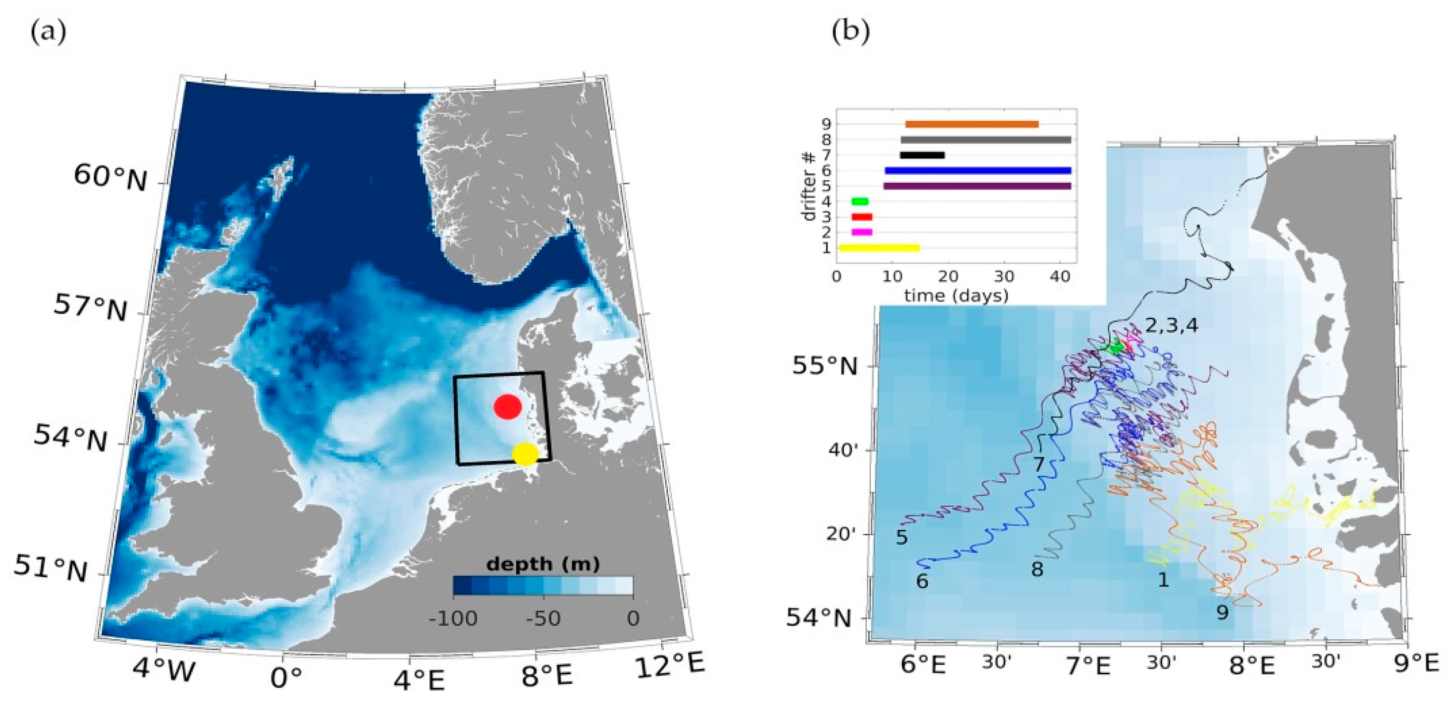
In a large and complex system such as the North Sea (Figure 1), minor perturbations may displace particles to very different drift regimes, causing strongly divergent particle trajectories [17]. Therefore, the particle distribution analysis is not intended to fully reproduce or explain the observations (the latter are extremely limited, particularly during extreme weather conditions). Instead, we aim to indicate the differences that can be due to wave-induced forcing processes. Although tide and wind-driven circulation in the North Sea seem to have been widely studied in the past, further research from a Lagrangian perspective with respect to coupling with waves and biogeochemical processes may be particularly relevant.
The importance of wave forcing for ocean circulation and sea-level predictions has been demonstrated [18,19,20,21,22,23], showing that the predictive skill of ocean circulation and sea level could be significantly enhanced by considering wave-induced processes. In extreme storm surge conditions over the North Sea, due to the strong non-linearity of wave–ocean–tidal interactions, wave–ocean coupling is considered to be significant for correct model predictions [18,24]. The impact of Stokes-related drift effects (Stokes–Coriolis forcing and Stokes drift advection on tracers and mass) were studied on the North Sea and Baltic Sea regions [25]. For tracer distribution and upwelling, the direct sea-state dependent momentum and energy fluxes are of higher importance than the Stokes drift processes implemented in the NEMO circulation model [23].
In this study, we investigate the role of wave-induced interaction processes in a fully coupled ocean–wind wave model system on Lagrangian transport modelling. Data from drifters deployed in the southern North Sea were used to assess the particle model simulations [26]. Lagrangian simulations were studied [27] based on the same drifter observations as in the present study and corresponding Lagrangian model simulations by using two circulation models. While only a stand-alone ocean model was used in the previous study [28], here, the same Ocean General Circulation Model (OGCM) is coupled to a wave model. The observational drifters [26] used to assess our simulations have previously been described in detail [27,29].
This paper is organized as follows. In Section 2, we describe the circulation, wave and Lagrangian transport models and the experimental setup. The evaluation of the model simulations is described in Section 3. Further, we assess the model results with direct comparisons of the simulations with the drifter data (Section 4). The drifter trajectories were modelled to investigate the importance of the wave effects, e.g., for search-and-rescue applications. We performed sensitivity experiments to investigate the impact of wave-induced forcing in the ocean model. The Lagrangian model used only the Eulerian current as provided by the hydrodynamical model simulations, by neglecting or considering the contributions from the Stokes drift or the wind drift corrections. The wave effects on the general circulation in the North Sea are studied. The paper ends with a discussion of the findings in Section 5 and the conclusions in Section 6.
2. Methods
2.1. Models and Set-Up
The Geesthacht coupled coastal model system (GCOAST) [30,31] was built upon a flexible and comprehensive coupled model system, integrating the most important key components of regional and coastal models. GCOAST encompasses (i) atmosphere-ocean–wave interactions, (ii) dynamics and fluxes in the land–sea transition, and (iii) coupling of the marine hydrosphere and biosphere. In our study, we used the GCOAST circulation, wave and drift model components to investigate the role of coupling in particle transport simulations in the North Sea. Those particles can be considered, for example, as simple representations of either oil fractions, fish larvae or search-and-rescue objects [32,33]. The wave–current interaction processes are momentum and energy sea state dependent fluxes, wave-induced mixing and Stokes–Coriolis forcing.
2.1.1. The Circulation Model NEMO
NEMO (Nucleus for European Modelling of the Ocean, [34]) is a framework of ocean-related computing engines, from which we use the OPA (Océan Parallélisé) package (for the ocean dynamics and thermodynamics) and the LIM3 (Louvain-la-Neuve Sea Ice Model) sea-ice dynamics and thermodynamics package [34]. In OPA, six primitive equations (momentum balance, the hydrostatic equilibrium, the incompressibility equation, the heat and salt conservation equations and an equation of state) are solved, where the Arakawa C grid is used in the horizontal. In the vertical, terrain-following coordinates, z coordinates or hybrid z-s coordinates can be chosen. Previously, NEMO was applied to the Baltic Sea and the North Sea area in uncoupled mode [35], coupled to atmospheric models [36] and forced with a wave model [18,19,25]. For the northwestern European Shelf, NEMO is used as a forecasting model in the COPERNICUS Marine Services [23,37,38]. The horizontal model resolution is about 2 nm with 51 σ-levels in the vertical providing instantaneous hourly surface (0.6 m uppermost level thickness) velocity fields. The study domain is 48.0–62.5° N and −4.7–13.2° E, which includes the North Sea, Skagerrak and Kattegat (Figure 1). The hourly atmospheric forcing is taken from subsequent short-range forecasts from the regional atmospheric model COSMO-EU, operated by the German Weather Service (DWD). Atmospheric pressure and tidal potential are included in the model forcing. River run-off is provided in the form of a daily climatology based on river discharge datasets. Lateral open boundary and initial condition fields (temperature, salinity, velocities and sea level) are derived from the MetOffice Forecasting Ocean Assimilation Model (FOAM) AMM7 (7 km horizontal resolution [23]), currently used by the Copernicus Marine Environment and Monitoring Service (CMEMS) as an operational service.
2.1.2. The Wave Model WAM
The wave model WAM [39,40] is a third-generation wave model, which solves the action balance equation without any a priori restriction on the evolution of spectrum. It is based on the spectral description of the wave conditions in frequency and directional space at each of the active model sea grid points of a certain model area. The version used in this study is the WAM Cycle 4.7, which is described in [41,42,43]. The source function integration scheme is made by [44], and the updated source terms of [45] are incorporated (Appendix A). The new version considers the wave-induced processes needed for coupling and are described in the next section. The spectrum in WAM is discretized with 24 directions and 25 frequencies. The wave model boundary information used at the open boundaries is taken from the regional wave model EWAM for Europe, which is run twice daily in operational routine at DWD.
2.1.3. Wave-Induced Processes
Ocean waves influence the circulation through a number of processes: turbulence due to breaking and non-breaking waves, momentum transfer from breaking waves to currents in deep and shallow water, wave interaction with planetary and local vorticity, Langmuir turbulence. The NEMO ocean model has been modified to take into account the following wave effects [11,18]: (1) the Stokes–Coriolis forcing; (2) sea-state dependent momentum flux, set as a scalar dependence of the flux from the atmosphere to waves and ocean or as a vector; and (3) a sea-state dependent energy flux. A description of the wave-induced forcing and the processes of wave interaction with the ocean circulation is given in Appendix A.1.
2.1.4. The Lagrangian Model
OpenDrift [46] is a freely available open-source off-line Lagrangian particle trajectory model that contains several modules for the advection of, e.g., oil spills [47], larvae and passive tracers [48]. For this study, the passive tracer module is used, which advects tracers only due to currents and winds. The sea and wind drift input is described in the next section. To investigate the influence of the wind, three different windage (referred to as leeway) coefficients when the bulk effect of waves and wind on the object is considered [32] (Lw) are used (0.1%, 0.5% and 1.0%). The real wind drag of the drifters is not known, so these values are used as estimates. The windage coefficients are multiplied by the wind velocity and added to the current velocity. The advection scheme is a 2nd-order Runge-Kutta scheme, and no additional diffusion is added because we only want to investigate the wave effects without any additional random “disturbances” [49]. Each particle thus follows a trajectory influenced by the sea surface currents and the equations read:
here x(t), y(t) are the particle displacements and u(t + t/2), v(t + t/2) are the horizontal velocity components at the particle’s position at t + t/2. If a particle reaches land, it is not further advected and considered beached. These particles are not further taken into account. If a particle leaves the domain through an open boundary, e.g., from the North Sea into the Atlantic, this particle is treated the same way. The model time step t and the particle seeding strategies are dependent on the specific experiment (provided in Section 3).
2.2. Observational Data
2.2.1. Drifter Data
The HE 445 cruise was performed between May and July 2015 (see Figure 1b for the trajectories and deployment period of the drifters) [26]. The R/V Heincke deployed nine Albatros drifters corresponding to two models (Figure S1): MD03i (drifters 1–6) and ODi (drifters 7–9). The drifters provided their current positions by a Global Positioning System (GPS), which were transmitted to the R/V Heincke via Iridium (a bi-directional satellite communication network). The MD03i is a cylinder-shaped drifter, with a diameter of 0.1 m and length of 0.32 m, but only approximately 0.08 m remains above the water surface. The MD03 drag ratio is 33.2, and according to the parametrization [26] the MD03 slippage is around 1.1 to 1.6 cm/s, for 10 m/s wind speed and velocity difference across the drogue (ΔU) equal to 0.1 cm/s. The ODi is a spherical drifter with a diameter of 0.2 m, but only approximately 0.1 m is above the water surface. A sail (0.5 m in length and diameter, Figure S1) was attached to every drifter to enhance the drag below the water surface, and it was 0.5 m below the surface. Due to the small drifter surface above the water compared to the sail surface below the water, the drifter is designed to follow the ambient current in the upper meter of the water column. Due to the meteorological conditions, only some of the drifters were recovered at the end of the campaign. The recovered drifters corresponded to the short data-set, while the non-recovered drifters from the long data-set transmitted data until the batteries drained (Figure 1b).
2.2.2. HF Radar Data
HFR surface current data were acquired by three radar stations in the German Bight [50,51]. The radar systems are based on linear antenna arrays installed near the shoreline. More details on the required processing can be found in [52]. For the considered system, the spatial radar resolution is 1.5 km in range. The radar system in the German Bight can reach out to about 120 km off the coast in favorable conditions and provides measurements with a 9 min averaging window every 20 min. The observations are available as interpolated to a 2 km Cartesian grid. Through a combination of the radial components from the different antenna stations, meridional and zonal current components can be derived; however, the original radial components were used for the subsequent data assimilation procedure. Further details of the system can be found in [51].
2.3. Model Experiments
For the control experiment (REF), the velocity is taken from the stand-alone circulation model NEMO (Section 2.1), and the wave–current interaction processes are not included. In the coupled wave-ocean experiments (CPL), the wave-induced processes described in Section 2.1.3 calculated by the wave model WAM are introduced in NEMO to simulate the Eulerian velocity, needed for the OpenDrift. We performed the following experiments, in which the individual or combined effects of the wave-induced processes are included: (i) sea state dependent momentum flux (CPL-TAUOC); (ii) Stokes–Coriolis forcing (CPL-STCOR) and (iii) both the sea state dependent momentum flux and the Stokes–Coriolis (CPL-TAUST).
In order to study the role of the windage, two additional sets of experiments have been performed. For these, in addition to the Eulerian velocity from REF and CPL experiments, the windage is included in OpenDrift. We will name these experiments WD-REF and WD-CPL, respectively. The different windage contributions that we consider are 0.1, 0.5 and 1% (WD-REF and WD-CPL with _0.1, _0.5, and _1.0, respectively). All experiments are summarized in Table 1.
3. Evaluation of Model Simulations
3.1. Methodology
The evaluation of the model results consisted of two parts. The first part (Section 3.2) aimed at studying the model runs statistically with direct comparisons of the simulations with the drifter data. In the follow-up part (Section 5), the drifter trajectories were modelled with OpenDrift to investigate the importance of the wave effects, e.g., for search-and-rescue applications.
The drifter velocities along the trajectories are calculated by dividing the distance between each drifter position by its time difference. The velocity is located in the middle between the two positions in time and space. Afterwards, the model velocities are interpolated trilinearly (lat, lon, time) to the drifter velocity positions and times. The root-mean-square error (rmse), standard deviation (std), bias (bia) and linear correlation coefficient (cor) are calculated to assess the model and drifter currents. Trilinear interpolation to the drifter position is performed for the wind and water depth and for each model experiment. For the analysis of meteorological conditions, periods with weak winds (25–27 June 2015) and strong southerly winds (01–03 June 2015) were chosen. In order to assign the errors of model velocities to different sources, a multi-linear regression was performed, solving the following equations:
Here, umodel is the model velocity, uwind is the wind velocity, denotes the velocity magnitude, i corresponds to the drifter number and a, b, c are the coefficients. Coefficient b represents direct windage acting on the GPS drifters. The coefficient a can indicate if the model under- or over-estimates surface velocity. Coefficient c includes deviations that cannot be explained by the model currents or the wind, like inaccurate directions; it can be considered an “offset”.
The drifter starting positions are used as initial positions in OpenDrift. In the trajectory simulations, the particles are initialized at the start location and start time of the Albatros drifters and move under the influence of the forcing until the real drifters expire. Drifter simulations of 25 h drift paths that were initialized every day from 0 to 53 at 13:00 UTC were previously performed [27]. It is important to stress that inall of our experiments, after starting the drifter simulations, we did not re-initialize the modelled drifters. The time steps in the OpenDrift experiments and the output frequency are both 10 min. In the first set of experiments, only the currents of REF and CPL were used in OpenDrift. To study the impact of the wind, REF and CPL current data were used together with the windage coefficients WD-REF and WD-CPL, respectively.
As a measure of the modelled trajectories, the skill score ss [4] is chosen. First, an index s is estimated as
where N is the total number of time steps, di is the distance of real and modelled drifter at time step i and loi is the total length of the trajectory of the real drifter at time step i. This index is used to calculate ss with
where n is the tolerance threshold, equal to 1 [4], which means that the cumulative separation distance is not larger than the cumulative trajectory length. If s and ss are close to 1, the modelled trajectory is close to the observed trajectory. It assumes that the model performance is better with higher ss and the cumulative separation distance is less significant than the cumulative trajectory length. If the skill score is close to zero, the model simulations have no skill.
The skill of the particle transport model depends on the quality of the ocean circulation, but the skill score has limitations [53]; e.g., in situations with small currents, it yields too small cumulative distances. It can thus give a too high estimate of s and a low skill score ss. To overcome these limitations, it has been suggested [4] to have an appropriate definition of the tolerance threshold n. In the German Bight study area, due to the strong tidal currents and wind forcing, the skill score can be an applicable measure for the drift model performance.
3.2. Surface Currents
3.2.1. HF-Radar versus Drifter Observations
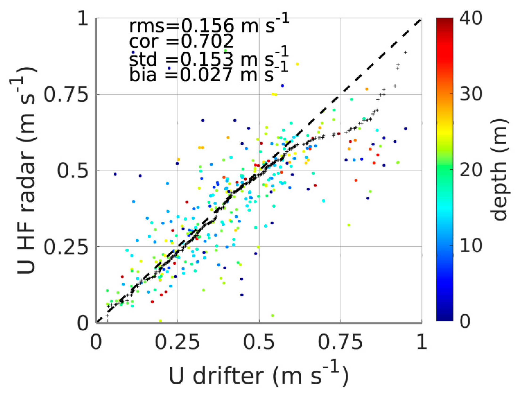
Figure 2 shows the drifter velocity magnitude versus the HF radar velocity as scatter plots generated for the whole period of drifter deployment. For the study period, 334 collocations of radar and drifter data were available for comparison. The velocity data of the drifters were filtered using a Savitzky–Golay filter [54] with a quadratic fit and a window length of ~2.3 days in order to remove outliers. The velocity of all nine drifters (regarding their deployment period or quality) was used in the scatter diagram to demonstrate the statistical robustness of the method. A detailed analysis of the separate trajectories of the Albatros drifters for the deployment periods was reported [27].
The HF radar currents should be interpreted as Eulerian currents [55] (i.e., without including the Stokes drift). However, it has also been argued that the HF radar velocity partially contains the Stokes drift, in which case the HF radar measurements contain a filtered component of the Stokes drift [56]. On the other side, comparisons of HF radar velocity measurements with drifter observations demonstrated that the presence of the Stokes drift in HF measurements is not settled. In Figure 2 and Figure S2 we compare HF radar velocities interpreted as Eulerian currents against the velocity estimated by the nine Albatros drifters. With a standard deviation of 15 cm/s and a bias of 2.7 cm/s, the drifter and the HF radar are in reasonably good agreement. A noticeable feature is a slight underestimation of HF velocity at higher values. There are several reasons for the disagreement between HF and drifters when the speed is over 0.6 m/s: (i) the HF radar retrieves the currents at a depth of around 1 m, but the drifter’s sails are located at 0.5 m. An underestimation of the HF radar regarding the drifter measurements may be expected. (ii) Due to strong wind stress during storm events, taking into account that the current profile over depth is logarithmic, a stronger current gradient between 1 m (HF) and 0.5 m (drifters) depth is expected. (iii) During breaking events in storm conditions, the drifter and the sail can surf over the sea surface, while the HF radar measures the current speed under the surface.
3.2.2. Assessment of Model Velocity
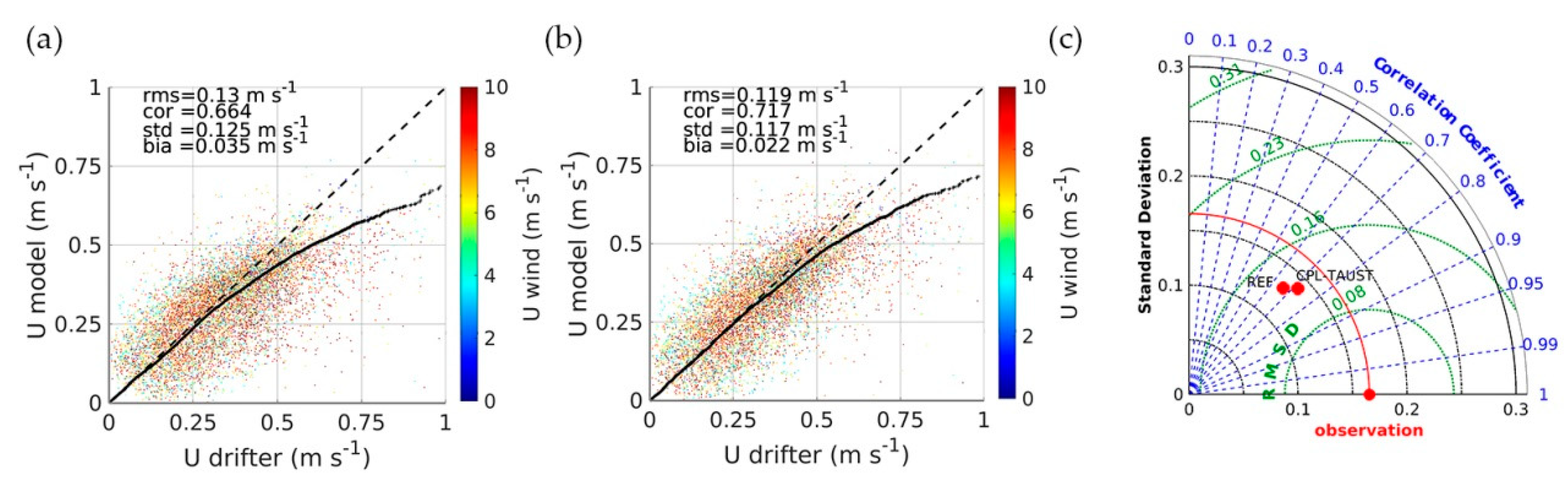
The simulated model velocities of the stand-alone NEMO (REF) and wave-circulation coupled model (CPL) are compared with the matching drifter velocity in Figure 3a. REF and CPL model velocities are well represented in the scatter plots and show good agreement with the drifter data. Above 30 cm/s, the modelled velocities are lower than the drifter velocities, as seen in the zonal and meridional components. The range of the q-q plot is smoother and fits better in moderate and high velocities in the coupled model simulations (Figure 3). The comparisons demonstrate a better fit of the meridional velocity to the observations by the coupled wave–current model for strong winds in both directions (Figure S3). The Taylor diagram shows a good agreement between both simulations and observations with slightly improved skills of the CPL experiments. It is noteworthy that despite the coarse resolution of the model and the complex bathymetry and coastline in our study area, the comparison is satisfying, and a general improvement of the surface currents in both directions is observed due to the wind–wave–ocean coupling. This is consistent with previous findings [21] in which coupled and stand-alone model circulation against Acoustic Doppler Current Profiler (ADCP) demonstrated an intensification of velocities due to coupling with waves, leading to a reduction in prediction errors.
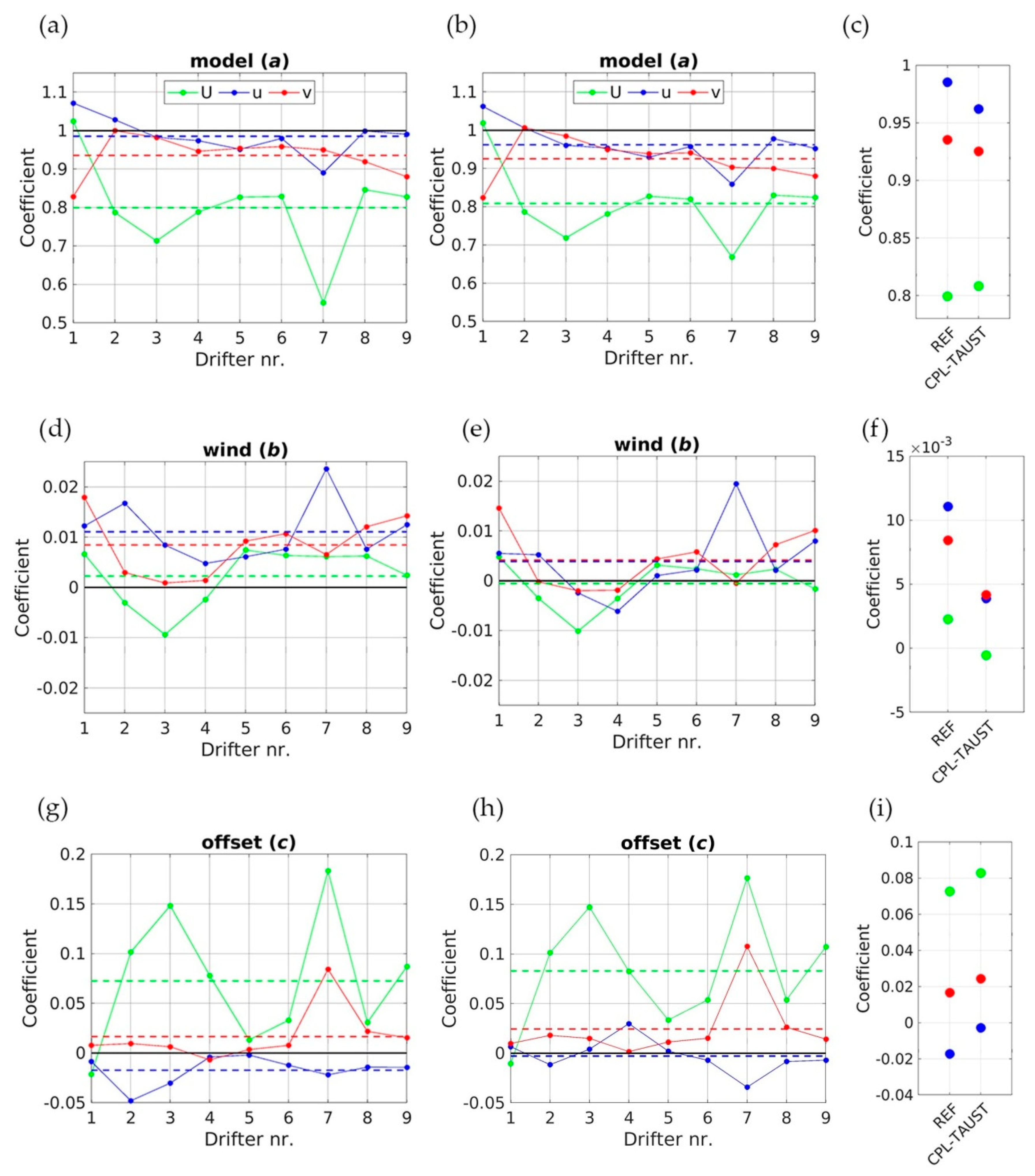
A multi-linear regression is performed, including model velocities, wind velocities and an offset to obtain insight into the error sources. Figure 4 shows these coefficients separately for each of the nine drifters. The model velocities are reduced in the zonal component by about 2.5% and in the meridional component by about 8%. While reducing the model velocities, the wind to be taken into account is around 1.0% for both velocity components. This value can also be interpreted as a guess about the wind drag of the drifters. For the same drifters, different windage and Stokes drift contributions were tested [27], in a combination of the Eulerian velocity of two hydrodynamic models. The parameterization used in [57] predicted a slippage of 1.1 to 1.6 cm/s for 10 m/s winds, and the expected windage should thus be close to 0.135%. However, as demonstrated in [58] this value depends strongly on the drifters and the chosen models and usually ranges between 0.1 and 1%. A wind drag of 0.27% was calculated from drifter surface ratio and 0.3% with Stokes drift was found to be the best combination in model simulations [49]. The offset of the zonal components is slightly negative (about −2 cm/s), while the offset of the meridional ones is slightly positive (about 2 cm/s).
By considering the wave coupling in the circulation model (Figure 4, right panels), the windage halves and model velocities are taken less into account. Instead, the offset increases. Note that drifter 7 shows substantial differences compared to the others, which may be due to technical problems. Drifters 1 and 9 also show increased/decreased coefficients. Together with drifter 7, these are the only drifters that are beached. A possible explanation is that the drogue was damaged during the storm and then landed on the beach. Thus, model uncertainties at the boundaries or grounding of drifters could be a possible reason.
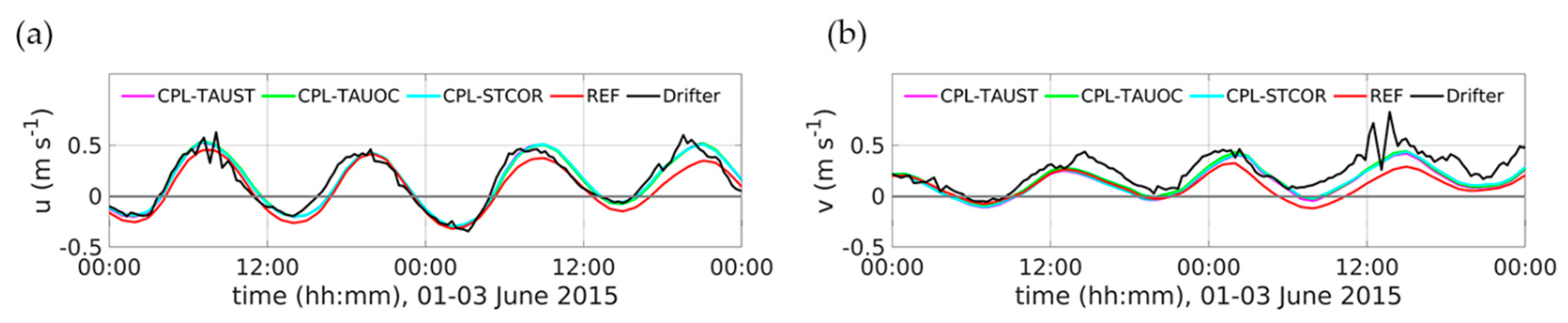
Figure 5 shows the time series for the chosen periods of drifter velocity and wind conditions for the stand-alone NEMO model and coupled model experiments considering wave-induced processes described in Section 2. The tidal cycle is simulated relatively well by all model experiments. There is a good fit between the observations and the model velocities during calm wind and wave conditions. The magnitude of the velocity in the CPL-TAUOC experiments is higher on 1 June than in REF, due to the veering of the wind, which influences the sea-state dependent momentum flux forcing. In periods of strong winds (e.g., 03/06), the velocity of the REF model is under-estimated, while the coupled NEMO-WAM currents performed better than the currents from the stand-alone NEMO mode. The wave model compares very well against in situ and satellite observations [43,59], see Figure S4.
4. Model Trajectories
We performed several Lagrangian experiments to investigate the impact of wave-induced forcing on the ocean model. In the first set of experiments, OpenDrift used only the Eulerian current fields as provided by NEMO (REF and CPL experiments) without adding any wind drift correction. In the second set of experiments, an additional windage was included.
4.1. Time Series of Separation Distance, Skill Scores and Standard Deviation
As a separation metric, the normalized cumulative Lagrangian separation [4] was applied. First, we focused on the model skill in drifter trajectories to demonstrate the impact of the local wind and wave-induced velocity correction terms. Further, we quantified the sensitivity of the simulated particles to the individual or combined effect of the wave-induced process that were implemented in our coupled wave-circulation model system.
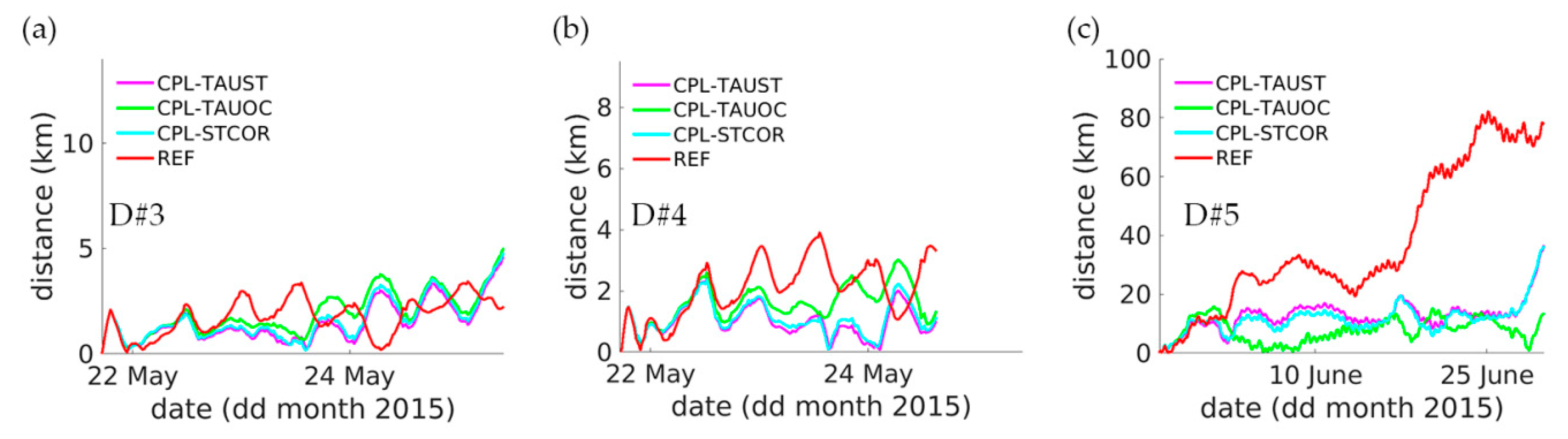
During the whole integration period, the separation distance of the drifters (Figure 6) remained very low, even though we did not perform any re-initialization of the drifter model after the initial release. Drifters 2–4 travelled for only a few days in the German Bight (Figure 1). It is noticeable that during the lifetime of these drifters, the simulated separation distance was kept within the model grid resolution. The model performance for drifters 5 and 6 (Figure S5) was high for all coupled experiments, and the separation distance was kept below 20 and 40 km, respectively, even one month after the start of integration. The separating distance of the REF (drifters 5–6) sharply increased after 20 June, showing significant deviation from the observations. This result coincides with earlier findings [27], demonstrating that on 16 and 22 June the wind direction sharply changed. Consequently, under these transitional conditions, signs of directional errors substantially differed, and the model performance was unsatisfactory. Implementing wave-induced processes into NEMO and using these Eulerian currents in OpenDrift led to a decrease in the separation distance between the CPL model experiments and the observations. In [18] was found that intensification of zonal velocity towards the coast, simulated by the coupled model, fits better with ADCP measurements. The present results show that for the CPL experiments, even during periods with moderate significant wave height, the inclusion of wave parameterizations improved the model performance. This demonstrates that separately adding a contribution of the Stokes drift to the Eulerian currents to OpenDrift in many cases might be insufficient to simulate the drifters under changing sea state conditions appropriately. The external Stokes drift can also be inconsistent with simulated ocean currents. For drifter 3 (Figure 6a), the distance error was of the same order as the resolution of our ocean model. For integration periods longer than a month, the distance error was less than twice the order of the grid resolution for the one-month simulation of drifter 5 (Figure 6c). Thus, the sea-state contribution of the momentum flux helps bring down the separation distance during most of the simulation periods.
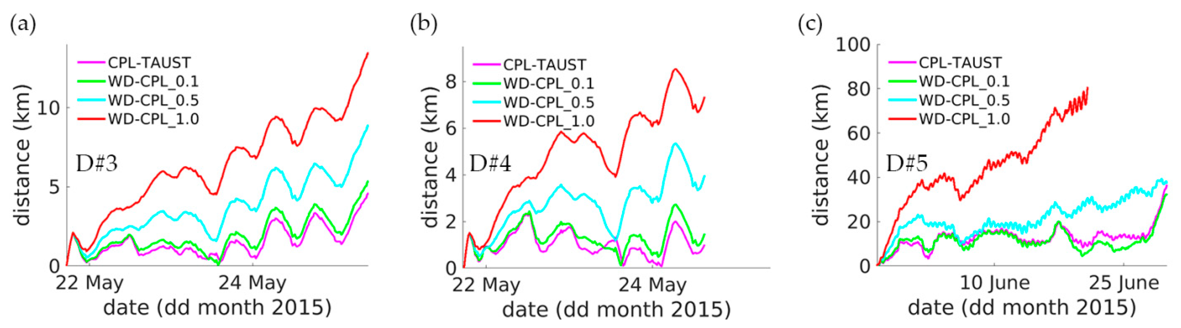
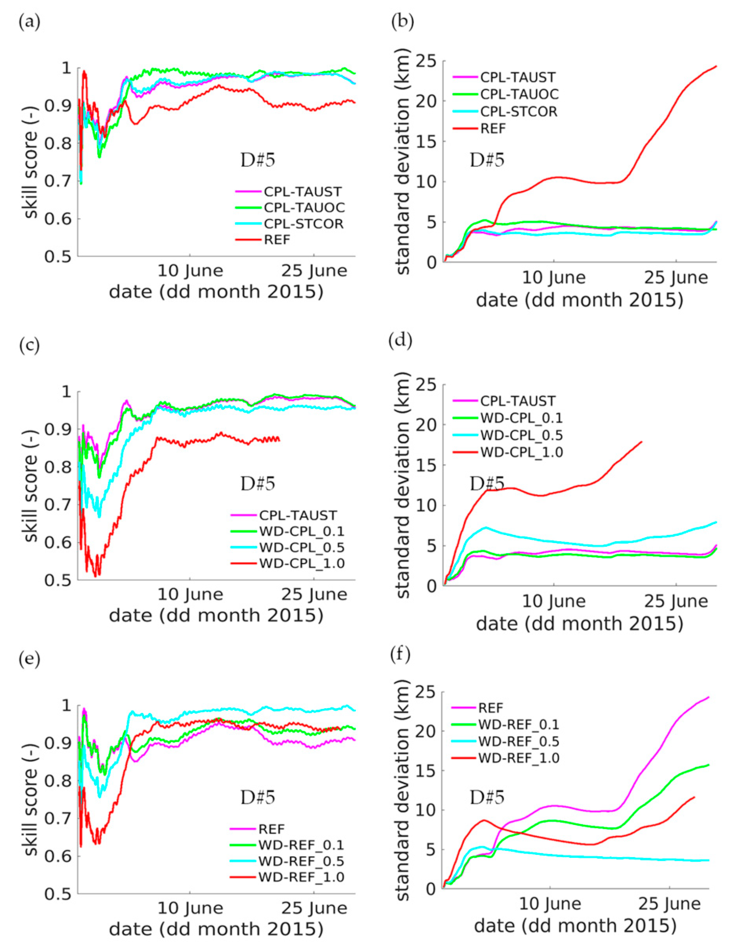
Sensitivity experiments on different wind drift (leeway) percentages (Figure 7 and Figure 8) demonstrated that only very few of them managed to reach higher skill scores than the CPL experiments. The results show the significance of producing the Eulerian velocity by the circulation models forced by sea state dependent momentum fluxes. The skill scores of the simulated drifters were generally high in all experiments, above 0.8 (Figure 9). The CPL experiments managed to keep the std low even after this period without considering any windage (see Figures S6–S8).
Applying wind drift correction of 0.5% or higher to WD-CPL experiments reduced the skill score (Figure 9c,d). In the first days of the integration period, the skill score of drifter #5 by windage correction of 0.5% and 1.0% dropped to 0.7 and 0.5, respectively. The skill score of the experiment with windage correction of 0.1% was closer to the CPL experiments but still slightly lower in the period from 26 May until 2 June (see also Figures S7 and S8). These differences were illustrated even better by the standard deviations of the WD-CPL experiments (Figure 9d). The standard deviations of D#5 stayed almost constant through the integration, at about 0.5 and 5 km, respectively, for CPL and WD-CPL plus 0.1% (Figure 9). Adding 0.5% windage yielded a higher standard deviation for all experiments. By assuming 1.0% windage, a trend of the systematic increase was observed for all drifters. Neither of the WD-CPL experiments (in Figure 9c,d) improved the skill scores and reduced the deviation between the trajectories of the Lagrangian model and observations by additionally considering the windage contribution to the Eulerian currents obtained by the coupled wave–circulation ocean model.
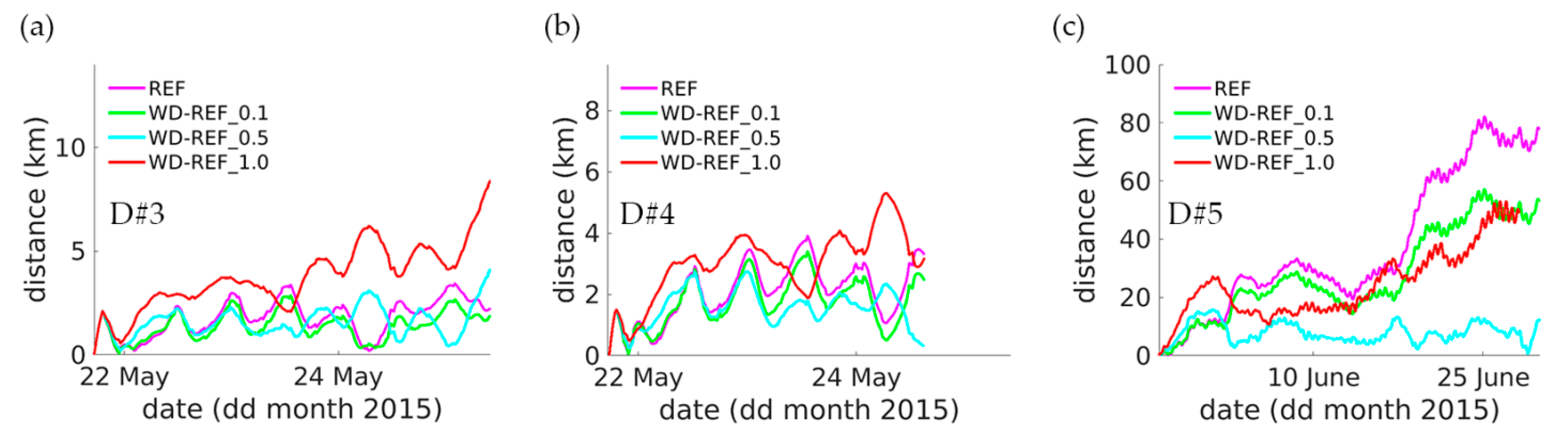
Sensitivity to the windage contribution was also determined for the REF runs (Figure 9e,f). The skill score and standard deviation of WD-REF were better than those of WD-CPL for all experiments. On the other side, the skill scores/standard deviations were lower/higher than those of CPL. Only by considering 0.5% windage of WD-REF are the ss and dd similar to the CPL.
It was demonstrated in [53] that simulated trajectories obtained by considering the wind drag of current velocities or the Stokes drift’s contribution showed better skills against the observations than without the corrections. They postulated that considering 1.0% windage or adding the contribution of the Stokes drift gives almost identical results. Our sensitivity analysis, however, showed that the CPL experiments performed best. From the rest of the experiments, only WD-REF with 0.5% windage provided similar skill. The model experiments showed that using Eulerian velocity estimated by considering Stokes–Coriolis and the sea state momentum provided similar results.
4.2. Particle Trajectories of the Albatros Drifters
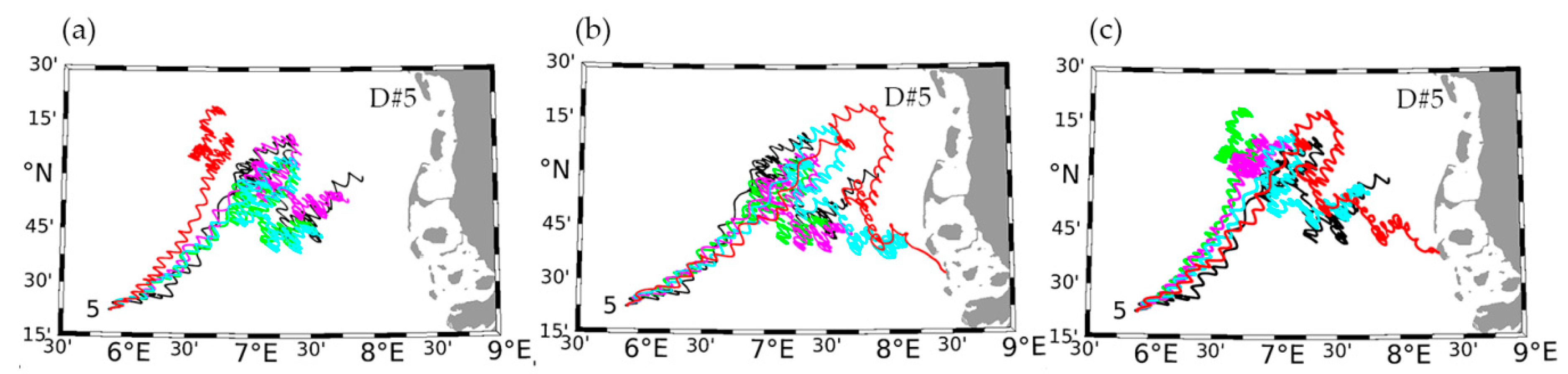
The trajectory of drifter 5 in the REF experiment deviated in a northwesterly direction. (Figure 10a) The trajectories obtained by the CPL experiments correctly reproduced the drifter direction and were in good agreement with observations. By north and northwesterly winds on 10 June and the anticyclonic circulation [27], the CPL experiments reproduced the windage of drifter 5 well. CPL-TAUOC separation distance was on the order of the model grid resolution (Figure 6). The low dd values remained until 29 June. The trajectory of WD-CPL_1.0 (Figure 10b) made a higher loop towards the north and northeast, deviating from the observations. By a 0.5% contribution of windage, the drifter was unrealistically transported towards the east and was beached. The trajectory of WD-CPL with 0.1% started deviating for 2.3 days after starting the simulation. WD-REF with 0.5% leeway showed a smaller separation distance (Figure 8), and the trajectory remained closer than that of WD-CPL with 0.5%. By adding 1.0% leeway, the simulated trajectories of WD-CPL and WD-REF can be considered as wrong. Skill scores and STDs for all experiments and during the deployment period of the drifters are given in Tables S1 and S2.
5. Discussion
Coupled ocean–wave models together with a Lagrangian transport model can be beneficial for drift and transport studies, ranging from search and rescue modelling of specific objects [33], backtracking [60], larval drift [61] and marine plastics [62,63] to the connectivity between different marine protected areas [16]. Accurate measures can potentially have a strong impact on biodiversity risk assessments (e.g., connected to marine litter or oil spills). In [16], several models of the North Sea were compared to study the variability and resulting uncertainty and differences between the models.
In our study, Eulerian currents from a coupled ocean-wave model were used to perform CPL and WD-CPL experiments. In this way, additional tuning of the contributing factors of the Stokes drift by the drifter model can be excluded in CPL experiments. Our results are in line with the study of [56]. The latter concluded that implementing the Stokes drift as a simple additive component of drift velocity, parameterized in terms of wind forcing, can be inconsistent (a violation of momentum and energy conservation) if Eulerian currents were simulated without taking into account the reservoir of wave momentum and energy. Our results indicate the relevance of the role of waves for redistribution of momentum, especially in periods of changing wind direction (Figure 6, Figure 7 and Figure 8).
The Eulerian currents in most of the Lagrangian transport models, e.g., for search and rescue operations, are taken from, for example, operational model output. The wind stress is parameterized to drive the dynamics of the upper ocean directly if the wave model is not included. However, part of the wind stress is supported by the flux of momentum from wind to waves. These processes were considered in our CPL-TAUOC and CPL-TAUST experiments to simulate the Eulerian velocity needed for OpenDrift. Due to the non-linearity of wave–current interactions, the individual effect of the wave-induced coupled STCOR and TAUOC processes are not superimposed on TAUST [18]. This result shows that the Eulerian currents by the coupled run provided the best fit to the observed particle trajectories. The worsening of the Lagrangian model skill, especially at the beginning of the drifter simulation, can have an impact on applications like search and rescue, in which skilled Lagrangian transport forecasts are needed at the very beginning of the operation. In summary, the use of additional wind corrections cannot be justified in WD-CPL experiments, since neither of the additional windage correction experiments demonstrated an improvement compared with the CPL experiments.
Displacements of the more offshore drifters, 5 and 6, were observed on 3–6 June [27], and the models turned out to be largely overestimated, concluding that neither simulated currents, windage fields nor Stokes drift by their Lagrangian model were able to reproduce the spatial gradients. In the present study, CPL experiments showed good agreement for these drifters with the observations. A deviation of the trajectory, and consequently an increase in the separating distance, was observed, but stayed within the same grid resolution. On the other side, the WD experiments deviations from the simulated drifter trajectories from the observations and separating distances were high. This result proves the importance of improving the Eulerian current simulations needed for Lagrangian transport modelling by implementing the sea state momentum forcing and Stokes–Coriolis forcing in the numerical model.
We did not aim to assess all specific differences between individual drifters and discuss in detail the wind forcing and the North Sea circulation during the different periods of their deployment, as this was done by [27]. Neither did we aim to tune the model to find the optimal percentage of the contribution of either the Stokes drift or windage that can be taken into account in OpenDrift simulations (as was recently done by [64]. Additional errors of the drifter simulations can be due to the errors in the atmospheric forcing, but also the boundary or tidal forcing. Another reason may be errors in the vertical resolution and mixing and bottom friction parameterization; the latter is essential for shallow water dynamics in regions like the German Bight. By using the same model configuration as in the present work, the interactions between barotropic tides and mesoscale processes were studied by [65] showing that barotropic tides affect diapycnal mixing substantially. In our study, we aimed to investigate the potential of a different approach, namely the contribution of wave-induced processes in the NEMO model.
It is important to stress here again that the North Sea circulation is very complex. The drifters were deployed in the shallow German Bight, a coastal ocean where the currents are dominated by tidal and wind forcing and are steered by the bathymetry and coastline. Other possible error sources are circulation features such as inertial oscillations, sub-mesoscale dynamics and baroclinic effects. Further studies are needed to quantify the combined effects of the mesoscale variability and resolution of the ocean and particle transport model, especially in the coastal areas of the German Bight (the Wadden Sea) as well as for other regions. For these aims, the GCOAST framework will be taken into account and tested for its best performance in terms of trajectory simulations over regions with different oceanographic properties (e.g., Baltic Sea, the North-East Atlantic).
The advantage of the method here is that by coupling the circulation model to the wave model, no further sensitivity experiments on the percentage of the contribution of windage or Stokes drift to improve the skills of the Lagrangian model are needed.
6. Conclusions
The results of our experiments lead us to the following conclusions:
1. Comparing currents from coupled and stand-alone model simulations demonstrated that the coupled model velocities fit better with the observations, especially moderate and high values. In calm wind and wave conditions, the differences are not pronounced. By using a fully coupled model, consistent atmosphere–wave–ocean forcing is applied to simulate the Eulerian currents needed for particle transport simulation. Besides, the bias of the directions in the wind–wave–ocean currents simulations is reduced compared to that in the stand-alone model. It is noteworthy that despite the coarse resolution of the NEMO model and the coupled NEMO-WAM setup and the complex bathymetry and coastline in our study area, the comparisons are satisfactory, also for the stand-alone model simulations. A general improvement in surface currents for both directions is observed due to the wind–wave–ocean coupling.
2. The multi-linear regression analysis showed that for CPL, windage is halved (from 1.0 to 0.5%), and the model velocities are taken less into account. Instead, the offset increases. These results show that the wind drift is better accounted for in the coupled NEMO-WAM model than in the stand-alone NEMO. It was also shown that the regression can reveal technical problems of the drifter, like probable drogue loss.
3. We showed the particle analysis by calculating values such as separating distance, skill score and standard deviation between model experiments and observations. We demonstrated that the skill score, based on the cumulative Lagrangian separation distance standardized by the associated cumulative trajectory length, proved to be a useful parameter to evaluate the overall model performance, rather than using a daily validation metric. Although the skill score and standard deviation of the ODi drifter are slightly lower than those of the MD03i, both types demonstrate good predictive skill. The MD03i drifter shows better skill for CPL than ODi. The skill scores with wind showed similar behavior by both types of drifters. For drifters that reached land, the model performance was low, which might be due to the insufficient model resolution and parameterization together with higher model uncertainty at the boundaries or beaching of drifters.
4. The skill scores and separation distances improved when wave-induced processes were taken into account in the ocean-only simulations. By considering sea state momentum dependencies or Stokes–Coriolis forcing in the coupled model, the skill scores are quite similar. Adding the contribution of windage or Stokes drift to currents produced by the fully coupled run with waves might lead to over-parameterization.
5. In the CPL experiments, it turned out that no additional tuning of the wind drift factor was needed for best fit with the observations. This also indicates that no additional contribution of windage or separate consideration of external Stokes drift was needed to predict the drifter trajectories satisfactorily. For some drifters, the skill scores of the WD-REF or WD-CPL experiments were similar to the CPL by adding a direct windage contribution to the REF. However, these percentages varied between different drifters and experiments.
The results based on the drifters used in this study showed that, in some cases, it might be favorable to implement full coupling of waves and circulation models to produce the currents needed for drifter simulations. This could lead to a more consistent approach instead of trying to tune the windage factor or percentage of external Stokes drift, separately or combined. Such tuning of the contribution coefficients is typically restricted by the need for availability and testing a large number of drifter observations (that are normally lacking), which is required to improve wind–wave–current forcing dependencies in the Lagrangian model. We note, however, that this conclusion is based on a limited period and a small area (over the German Bight). Nevertheless, the model simulations showed that the results are promising for better understanding and prediction of Lagrangian transport by using Eulerian currents simulated by coupled wave–ocean model simulations instead of a stand-alone ocean model. The results revealed that the newly introduced wave effects are essential for the drift model performance.
Supplementary Materials
The following are available online at https://www.mdpi.com/2073-4441/13/4/415/s1, Table S1: Skill score over the deployment period of drifter; Table S2: STDs average over the deployment period of stds (km); Figure S1. (a)The experiment site in the German Bight (a). The shaded colours show the number of the HF radar measurements from the three radar antennas. The trajectories of the drifter #1–9 are plotted with the colour lines. Sail illustration of the MD03i frifter (b); MD03i (drifter #1–6) (c) and ODi (drifter 7–9)-HZG drifters (d). Figure S2. Zonal (a) and meridional (b) velocity scatter plots: drifter versus HF radar data (m/s). The black dots indicate the quantile-quantile (q-q) plot. The black dashed line is the diagonal. The model topography is also interpolated to the drifter positions and depicted with colours. Figure S3. Scatter plots of velocity magnitude, as well as of the zonal and meridional components for the REF experiment (a), (d) and (g), (and CPL-TAUST experiment (b), (e) and (h) of the HZG drifters vs. model data coloured to wind velocity and the quantile-quantile (q-q) plot in black. The black dashed line is the diagonal. Taylor Diagram of the velocity magnitude, as well as of the zonal and meridional components (c), (f) and (i). Figure S4. Significant wave heights (m) at Elbe (top) and FINO-3 (bottom) buoy station in in May and June 2015. The blue dots are the in-situ observations; the red line corresponds to the WAM simulations. For the position see Figure 1a. Figure S5. Time series of the distance (km) between the observed and model drifter #1–9 (a–i), # trajectories of REF (red line), CPL-TAUOC (green line), CPL-TAUST (magenta line) and CPL-STCOR (blue line) experiments. Figure S6. Time series of the skill score and the standard deviation of the distance (km) between the observed and model drifter #3–9 (a–f) trajectories of the REF (red line), CPL-TAUOC (green line), CPL-TAUST (magenta line) and CPL-STCOR (blue line) experiments. Figure S7. Time series of the skill score and the standard deviation of the distance (km) between the observed and model drifter #3–9 (a–f) trajectories of the WD-CPL experiments with wind drag contribution of 0.1, 0.5 and 1.0%. Figure S8. Time series of the skill score and the standard deviation of the distance (km) between the observed and model drifter #3–9 (a–f) trajectories of the WD-REF experiments with wind drag contribution of 0.1, 0.5 and 1.0%.
Author Contributions
J.S. conceived the study and wrote major parts of the manuscript. M.R. conducted the model simulations and provided parts of the text, R.C.A. made the GPS drifter experiments, provided their data and contributed to their description. Ø.B. helped develop the model coupling and contributed to the manuscript. C.S. contributed to discussion. J.S. and Ø.B. contributed to the project administration. All authors have read and agreed to the published version of the manuscript.
Funding
J.S. and Ø.B. gratefully acknowledge funding from CMEMS through the Service Evolution 2 project WaveFlow. Ø.B. is grateful for funding from the Joint Rescue Coordination Centres which has helped fund the development of the OpenDrift model. The Research Council of Norway has also helped fund the development of OpenDrift through the projects CIRFA (grant no. 237906) and Retrospect (grant no. 244262). M.R. has been supported by the project “Macroplastics Pollution in the Southern North Sea–Sources, Pathways and Abatement Strategies” (grant no. ZN3176) funded by the German Federal State of Lower Saxony. C.S. and J.S acknowledge the funding by Initiative and Networking Fund of the Helmholtz Association through the project “Advanced Earth System Modelling Capacity (ESM)” and CLICCS Center of Excellence, J.S. is grateful for funding from BMBF bilateral project “Ocean Currents_MoDA” (grant no: 03F0822A).
Data Availability Statement
The raw data of observed drifter locations are freely available from [26]. German Weather Service data are available from: https://opendata.dwd.de/weather/nwp/icon-eu/grib/. The HF-radar data are available through the Coastal Observing System for Northern and Arctic seas (COSYNA) [54,55]. OpenDrift [46] is a freely available open-source off-line Lagrangian particle trajectory model.
Acknowledgments
The authors thank the UK Met Office for providing the NEMO model setup. We thank Arno Behrens, Oliver Krüger and Sebastian Grayek for technical support with the models. We thank to Gerhard Gayer for the wave model validations. We are thankful to Sabine Hartmann or technical support with the figures. We appreciate the use of the German Weather Service (DWD) atmospheric data, provided by the German Weather Service.
Conflicts of Interest
The authors declare that there are no conflict of interest.
Appendix A
Appendix A.1. Wave–Current Interaction Processes
As described in Section 2, the NEMO ocean model has been modified to take into account the following wave effects [11,18]: (1) the Stokes–Coriolis forcing; (2) sea-state dependent momentum flux, set as a scalar dependence of the flux from the atmosphere to waves and ocean or as a vector; and (3) a sea-state dependent energy flux. Below is the description of the wave-induced forcing and the processes of wave interaction with the ocean circulation.
Stokes Drift
The surface Stokes drift ust is defined by the following integral expression in the WAM model:
Here E = E() is the two-dimensional wave spectrum which gives the energy distribution of the ocean waves over angular frequency ω and propagation direction θ. Particle trajectories in water waves do not form entirely closed orbits because the particles spend more time forward under wave crests than backwards under wave troughs. This sets up a second-order effect, which leads to a discrepancy between the average Lagrangian flow velocity of a fluid parcel and the Eulerian flow velocity known as the Stokes drift. As is the case for the wind-induced currents, the Stokes drift also interacts with the Earth’s rotation. This adds an additional veering to the ocean currents known as the Stokes–Coriolis force [66],
where is the Stokes drift vector, p is the pressure, is the surface stress and is the upward unit vector. Because calculating the full vertical profile is costly, the Stokes drift velocity profile was first calculated with an approximation from [10]. The Stokes–Coriolis force is also included in the tracer advection equations as described by [28]. In the present approach, the Stokes drift velocity profile is also considered [67,68].
Appendix A.2. Momentum and Energy Flux from the Wave Model
Provided that current gradients are sufficiently weak, the energy and momentum fluxes can be calculated from the energy balance equation (with an approximation from [36]:
where E = E(ω,θ) is the two-dimensional wave spectrum which gives the energy distribution of the ocean waves over angular frequency ω and propagation direction θ, vg is the group velocity. On the right-hand side of the action balance equation are the source terms that represent physical processes which generate, redistribute or dissipate wave energy in the WAM model. These terms denote, respectively, wave growth by the wind , non-linear transfer of wave energy through four-wave interactions and wave dissipation caused by white capping and bottom friction . In the present calculations, we also took into account depth-induced wave breaking .
Making use of the energy balance in the Equation (A4) the wave-induced stress is given by
while the dissipation stress is given by
Similarly, the energy flux from wind to waves is given by
and the energy flux from waves to the ocean, Φdiss, is defined as
Under stationary and homogenous conditions the momentum and energy balance reduces to
and
The momentum flux to the ocean column, denoted by τoc, is the sum of the flux transferred by turbulence across the air–sea interface which was not used to generate waves τa − τin and the momentum flux transferred by the ocean waves due to wave breaking τdiss. This leads to
The contribution to the energy flux is
It is important to note that while the momentum fluxes are mainly determined by the high-frequency part of the wave spectrum, the energy flux is to some extent also determined by the low-frequency waves.
The high frequency (ω > ωc) contribution to the energy flux (first term of Equation (A11)) is
In NEMO, the wave-induced turbulent kinetic energy (TKE) flux introduced at the sea surface depends on the wave energy factor α [69] and is set to a constant value regardless of the sea state. Authors in [69] argued that the turbulent kinetic energy flux is relatively insensitive to the sea state and is well approximated by αu3w* (uw* is the water-side friction velocity), and α = 100 was thought to be representative of a mid-range of sea states between young wind seas and fully developed situations. As shown above, using the full spectral wave model, it is possible to estimate both the momentum energy and energy fluxes directly from the wave breaking source terms [11,18,25].
References
- Van Sebille, E.; Griffies, S.M.; Abernathey, R.; Adams, T.P.; Berloff, P.; Biastoch, A.; Blanke, B.; Chassignet, E.P.; Cheng, Y.; Cotter, C.J.; et al. Lagrangian Ocean Analysis: Fundamentals and Practices. Ocean Modell. 2018, 121, 49–75. [Google Scholar] [CrossRef]
- Van Sebille, E.; Aliani, S.; Law, K.L.; Maximenko, N.; Alsina, J.M.; Bagaev, A.; Bergmann, M.; Chapron, B.; Chubarenko, I.; Cózar, A.; et al. The Physical Oceanography of the Transport of Floating Marine Debris. Environ. Res. Lett. 2020, 15, 023003. [Google Scholar] [CrossRef] [Green Version]
- Van Sebille, E.; van Leeuwen, P.J.; Biastoch, A.; Barron, C.N.; de Ruijter, W.P.M. Lagrangian Validation of Numerical Drifter Trajectories Using Drifting Buoys: Application to the Agulhas System. Ocean Modell. 2009, 29, 269–276. [Google Scholar] [CrossRef] [Green Version]
- Liu, Y.; Weisberg, R.H. Evaluation of Trajectory Modeling in Different Dynamic Regions Using Normalized Cumulative Lagrangian Separation. J. Geophys. Res. Oceans 2011, 116. [Google Scholar] [CrossRef] [Green Version]
- Sotillo, M.G.; Fanjul, E.A.; Castanedo, S.; Abascal, A.J.; Menendez, J.; Emelianov, M.; Olivella, R.; García-Ladona, E.; Ruiz-Villarreal, M.; Conde, J.; et al. Towards an Operational System for Oil-Spill Forecast over Spanish Waters: Initial Developments and Implementation Test. Mar. Pollut. Bull. 2008, 56, 686–703. [Google Scholar] [CrossRef]
- Huntley, H.S.; Lipphardt, B.L.; Kirwan, A.D. Lagrangian Predictability Assessed in the East China Sea. Ocean Modell. 2011, 36, 163–178. [Google Scholar] [CrossRef]
- Janssen, P.A.E.M. Wave-Induced Stress and the Drag of Air Flow over Sea Waves. J. Phys. Oceanogr. 1989, 19, 745–754. [Google Scholar] [CrossRef] [Green Version]
- Janssen, P.A.E.M. Quasi-Linear Theory of Wind-Wave Generation Applied to Wave Forecasting. J. Phys. Oceanogr. 1991, 21, 1631–1642. [Google Scholar] [CrossRef] [Green Version]
- Semedo, A.; Saetra, Ø.; Rutgersson, A.; Kahma, K.K.; Pettersson, H. Wave-Induced Wind in the Marine Boundary Layer. J. Atmos. Sci. 2009, 66, 2256–2271. [Google Scholar] [CrossRef] [Green Version]
- Breivik, Ø.; Janssen, P.A.E.M.; Bidlot, J.-R. Approximate Stokes Drift Profiles in Deep Water. J. Phys. Oceanogr. 2014, 44, 2433–2445. [Google Scholar] [CrossRef] [Green Version]
- Breivik, Ø.; Mogensen, K.; Bidlot, J.-R.; Balmaseda, M.A.; Janssen, P.A.E.M. Surface Wave Effects in the NEMO Ocean Model: Forced and Coupled Experiments. J. Geophys. Res. Ocean. 2015, 120, 2973–2992. [Google Scholar] [CrossRef] [Green Version]
- Guan, C.; Xie, L. On the Linear Parameterization of Drag Coefficient over Sea Surface. J. Phys. Oceanogr. 2004, 34, 2847–2851. [Google Scholar] [CrossRef]
- Wu, L.; Rutgersson, A.; Sahlée, E.; Larsén, X.G. Swell Impact on Wind Stress and Atmospheric Mixing in a Regional Coupled Atmosphere-Wave Model. J. Geophys. Res. Ocean. 2016, 121, 4633–4648. [Google Scholar] [CrossRef] [Green Version]
- Higgins, C.; Vanneste, J.; Bremer, T.S. Unsteady Ekman-Stokes Dynamics: Implications for Surface Wave-Induced Drift of Floating Marine Litter. Geophys. Res. Lett. 2020, 47. [Google Scholar] [CrossRef]
- Röhrs, J.; Christensen, K.H.; Hole, L.R.; Broström, G.; Drivdal, M.; Sundby, S. Observation-Based Evaluation of Surface Wave Effects on Currents and Trajectory Forecasts. Ocean Dyn. 2012, 62, 1519–1533. [Google Scholar] [CrossRef]
- Hufnagl, M.; Payne, M.; Lacroix, G.; Bolle, L.J.; Daewel, U.; Dickey-Collas, M.; Gerkema, T.; Huret, M.; Janssen, F.; Kreus, M.; et al. Variation That Can Be Expected When Using Particle Tracking Models in Connectivity Studies. J. Sea Res. 2017, 127, 133–149. [Google Scholar] [CrossRef] [Green Version]
- Röhrs, J.; Christensen, K.H.; Vikebø, F.; Sundby, S.; Saetra, Ø.; Broström, G. Wave-Induced Transport and Vertical Mixing of Pelagic Eggs and Larvae. Limnol. Oceanogr. 2014, 59, 1213–1227. [Google Scholar] [CrossRef]
- Staneva, J.; Alari, V.; Breivik, Ø.; Bidlot, J.-R.; Mogensen, K. Effects of Wave-Induced Forcing on a Circulation Model of the North Sea. Ocean Dyn. 2017, 67, 81–101. [Google Scholar] [CrossRef]
- Alari, V.; Staneva, J.; Breivik, Ø.; Bidlot, J.-R.; Mogensen, K.; Janssen, P. Surface Wave Effects on Water Temperature in the Baltic Sea: Simulations with the Coupled NEMO-WAM Model. Ocean Dyn. 2016, 66, 917–930. [Google Scholar] [CrossRef]
- Brown, J.M.; Bolaños, R.; Wolf, J. The Depth-Varying Response of Coastal Circulation and Water Levels to 2D Radiation Stress When Applied in a Coupled Wave–Tide–Surge Modelling System during an Extreme Storm. Coast. Eng. 2013, 82, 102–113. [Google Scholar] [CrossRef] [Green Version]
- Brown, J.M.; Wolf, J. Coupled Wave and Surge Modelling for the Eastern Irish Sea and Implications for Model Wind-Stress. Cont. Shelf Res. 2009, 29, 1329–1342. [Google Scholar] [CrossRef] [Green Version]
- Staneva, J.; Wahle, K.; Koch, W.; Behrens, A.; Fenoglio-Marc, L.; Stanev, E.V. Coastal Flooding: Impact of Waves on Storm Surge during Extremes—A Case Study for the German Bight. Nat. Hazards Earth Syst. Sci. 2016, 16, 2373–2389. [Google Scholar] [CrossRef] [Green Version]
- Lewis, H.W.; Castillo Sanchez, J.M.; Siddorn, J.; King, R.R.; Tonani, M.; Saulter, A.; Sykes, P.; Pequignet, A.-C.; Weedon, G.P.; Palmer, T.; et al. Can Wave Coupling Improve Operational Regional Ocean Forecasts for the North-West European Shelf? Ocean Sci. 2019, 15, 669–690. [Google Scholar] [CrossRef] [Green Version]
- Cavaleri, L.; Abdalla, S.; Benetazzo, A.; Bertotti, L.; Bidlot, J.-R.; Breivik, Ø.; Carniel, S.; Jensen, R.E.; Portilla-Yandun, J.; Rogers, W.E.; et al. Wave Modelling in Coastal and Inner Seas. Prog. Oceanogr. 2018, 167, 164–233. [Google Scholar] [CrossRef]
- Wu, L.; Breivik, Ø.; Rutgersson, A. Ocean-Wave-Atmosphere Interaction Processes in a Fully Coupled Modeling System. J. Adv. Modeling Earth Syst. 2019, 11, 3852–3874. [Google Scholar] [CrossRef] [Green Version]
- Carrasco, R.; Horstmann, J. German Bight Surface Drifter Data from Heincke Cruise HE 445. 2015. Available online: https://doi.pangaea.de/10.1594/PANGAEA.874511 (accessed on 28 January 2020).
- Callies, U.; Groll, N.; Horstmann, J.; Kapitza, H.; Klein, H.; Maßmann, S.; Schwichtenberg, F. Surface Drifters in the German Bight: Model Validation Considering Windage and Stokes Drift. Ocean Sci. 2017, 13, 799–827. [Google Scholar] [CrossRef] [Green Version]
- Ricker, M.; Stanev, E.V. Circulation of the European Northwest Shelf: A Lagrangian Perspective. Ocean Sci. 2020, 16, 637–655. [Google Scholar] [CrossRef]
- Callies, U.; Carrasco, R.; Floeter, J.; Horstmann, J.; Quante, M. Submesoscale Dispersion of Surface Drifters in a Coastal Sea near Offshore Wind Farms. Ocean Sci. 2019, 15, 865–889. [Google Scholar] [CrossRef] [Green Version]
- Von Schuckmann, K.; Traon, P.-Y.L.; Smith, N.; Pascual, A.; Djavidnia, S.; Gattuso, J.-P.; Grégoire, M.; Nolan, G.; Aaboe, S.; Aguiar, E.; et al. Copernicus Marine Service Ocean State Report, Issue 3. J. Oper. Oceanogr. 2019, 12, S1–S123. [Google Scholar] [CrossRef]
- Ho-Hagemann, H.T.M.; Hagemann, S.; Grayek, S.; Petrik, R.; Rockel, B.; Staneva, J.; Feser, F.; Schrum, C. Internal Model Variability of the Regional Coupled System Model GCOAST-AHOI. Atmosphere 2020, 11, 227. [Google Scholar] [CrossRef] [Green Version]
- Breivik, Ø.; Allen, A.A. An Operational Search and Rescue Model for the Norwegian Sea and the North Sea. J. Mar. Syst. 2008, 69, 99–113. [Google Scholar] [CrossRef] [Green Version]
- Breivik, Ø.; Allen, A.A.; Maisondieu, C.; Olagnon, M. Advances in Search and Rescue at Sea. Ocean Dyn. 2013, 63, 83–88. [Google Scholar] [CrossRef] [Green Version]
- Madec, G. Note du Pôle de modélisation, Institut Pierre-Simon Laplace (IPSL); NEMO Ocean Engine: Paris, France, 2008. [Google Scholar]
- Hordoir, R.; Axell, L.; Höglund, A.; Dieterich, C.; Fransner, F.; Gröger, M.; Liu, Y.; Pemberton, P.; Schimanke, S.; Andersson, H.; et al. Nemo-Nordic 1.0: A NEMO-Based Ocean Model for the Baltic and North Seas—Research and Operational Applications. Geosci. Model Dev. 2019, 12, 363–386. [Google Scholar] [CrossRef] [Green Version]
- Dietrich, J.C.; Zijlema, M.; Westerink, J.J.; Holthuijsen, L.H.; Dawson, C.; Luettich, R.A.; Jensen, R.E.; Smith, J.M.; Stelling, G.S.; Stone, G.W. Modeling Hurricane Waves and Storm Surge Using Integrally-Coupled, Scalable Computations. Coast. Eng. 2011, 58, 45–65. [Google Scholar] [CrossRef]
- O’Dea, E.; Furner, R.; Wakelin, S.; Siddorn, J.; While, J.; Sykes, P.; King, R.; Holt, J.; Hewitt, H. The CO5 Configuration of the 7 km Atlantic Margin Model: Large-Scale Biases and Sensitivity to Forcing, Physics Options and Vertical Resolution. Geosci. Model Dev. 2017, 10, 2947–2969. [Google Scholar] [CrossRef] [Green Version]
- O’Dea, E.J.; Arnold, A.K.; Edwards, K.P.; Furner, R.; Hyder, P.; Martin, M.J.; Siddorn, J.R.; Storkey, D.; While, J.; Holt, J.T.; et al. An Operational Ocean Forecast System Incorporating NEMO and SST Data Assimilation for the Tidally Driven European North-West Shelf. J. Oper. Oceanogr. 2012, 5, 3–17. [Google Scholar] [CrossRef] [Green Version]
- Group, T.W. The WAM Model—A Third Generation Ocean Wave Prediction Model. J. Phys. Oceanogr. 1988, 18, 1775–1810. [Google Scholar] [CrossRef] [Green Version]
- ECMWF. IFS Documentation CY40R1; IFS Documentation; ECMWF: Readink, UK, 2014. [Google Scholar]
- Komen, G.J.; Cavaleri, L.; Donelan, M.; Hasselmann, K.; Hasselmann, S.; Janssen, P.A.E.M. Dynamics and Modelling of Ocean Waves; Cambridge University Press: Cambridge, UK, 1994; ISBN 978-0-521-57781-6. [Google Scholar]
- Günther, H.; Hasselmann, S.; Janssen, P.A.E.M. The WAM Model Cycle 4.0; Deutsches Klimarechenzentrum: Hamburg, Germany, 1992; p. 102. [Google Scholar]
- Staneva, J.; Behrens, A.; Wahle, K. Wave Modelling for the German Bight Coastal-Ocean Predicting System. J. Phys. Conf. Ser. 2015, 633, 012117. [Google Scholar] [CrossRef]
- Hersbach, H.; Janssen, P.A.E.M. Improvement of the Short-Fetch Behavior in the Wave Ocean Model (WAM). J. Atmos. Ocean. Technol. 1999, 16, 884–892. [Google Scholar] [CrossRef]
- Bidlot, J.-R.; Janssen, P.; Abdalla, S. A Revised Formulation of Ocean Wave Dissipation and Its Model Impact; ECMWF: Reading, UK, 2007; p. 27. [Google Scholar]
- Dagestad, K.-F.; Röhrs, J.; Breivik, Ø.; Ådlandsvik, B. OpenDrift v1.0: A Generic Framework for Trajectory Modelling. Geosci. Model Dev. 2018, 11, 1405–1420. [Google Scholar] [CrossRef] [Green Version]
- Jones, C.E.; Dagestad, K.-F.; Breivik, Ø.; Holt, B.; Röhrs, J.; Christensen, K.H.; Espeseth, M.; Brekke, C.; Skrunes, S. Measurement and Modeling of Oil Slick Transport. J. Geophys. Res. Ocean. 2016, 121, 7759–7775. [Google Scholar] [CrossRef]
- Christensen, K.H.; Breivik, Ø.; Dagestad, K.-F.; Röhrs, J.; Ward, B. Short-Term Predictions of Oceanic Drift. Oceanography 2018, 31, 59–67. [Google Scholar] [CrossRef]
- Meyerjürgens, J.; Badewien, T.H.; Garaba, S.P.; Wolff, J.-O.; Zielinski, O. A State-of-the-Art Compact Surface Drifter Reveals Pathways of Floating Marine Litter in the German Bight. Front. Mar. Sci. 2019, 6. [Google Scholar] [CrossRef] [Green Version]
- Baschek, B.; Schroeder, F.; Brix, H.; Riethmüller, R.; Badewien, T.H.; Breitbach, G.; Brügge, B.; Colijn, F.; Doerffer, R.; Eschenbach, C.; et al. The Coastal Observing System for Northern and Arctic Seas (COSYNA). Ocean Sci. 2017, 13, 379–410. [Google Scholar] [CrossRef] [Green Version]
- Stanev, E.V.; Schulz-Stellenfleth, J.; Staneva, J.; Grayek, S.; Grashorn, S.; Behrens, A.; Koch, W.; Pein, J. Ocean Forecasting for the German Bight: From Regional to Coastal Scales. Ocean Sci. 2016, 12, 1105–1136. [Google Scholar] [CrossRef] [Green Version]
- Gurgel, K.W. Remarks on Signal Processing in HF Radars Using FMCW Modulation. IRS 2009, 63–67. Available online: http://wera.cen.uni-hamburg.de/pub_70.pdf (accessed on 28 January 2020).
- De Dominicis, M.; Pinardi, N.; Zodiatis, G.; Archetti, R. MEDSLIK-II, a Lagrangian Marine Surface Oil Spill Model for Short-Term Forecasting – Part 2: Numerical Simulations and Validations. Geosci. Model Dev. 2013, 6, 1871–1888. [Google Scholar] [CrossRef] [Green Version]
- Savitzky, A.; Golay, M.J.E. Smoothing and Differentiation of Data by Simplified Least Squares Procedures. Anal. Chem. 1964, 36, 1627–1639. [Google Scholar] [CrossRef]
- Röhrs, J.; Sperrevik, A.K.; Christensen, K.H.; Broström, G.; Breivik, Ø. Comparison of HF Radar Measurements with Eulerian and Lagrangian Surface Currents. Ocean Dyn. 2015, 65, 679–690. [Google Scholar] [CrossRef] [Green Version]
- Ardhuin, F.; Marié, L.; Rascle, N.; Forget, P.; Roland, A. Observation and Estimation of Lagrangian, Stokes, and Eulerian Currents Induced by Wind and Waves at the Sea Surface. J. Phys. Oceanogr. 2009, 39, 2820–2838. [Google Scholar] [CrossRef]
- Niiler, P.P.; Sybrandy, A.S.; Bi, K.; Poulain, P.M.; Bitterman, D. Measurements of the Water-Following Capability of Holey-Sock and TRISTAR Drifters. Deep Sea Res. Part I Oceanogr. Res. Pap. 1995, 42, 1951–1964. [Google Scholar] [CrossRef]
- Stanev, E.V.; Badewien, T.H.; Freund, H.; Grayek, S.; Hahner, F.; Meyerjürgens, J.; Ricker, M.; Schöneich-Argent, R.I.; Wolff, J.-O.; Zielinski, O. Extreme Westward Surface Drift in the North Sea: Public Reports of Stranded Drifters and Lagrangian Tracking. Cont. Shelf Res. 2019, 177, 24–32. [Google Scholar] [CrossRef]
- Wiese, A.; Staneva, J.; Schulz-Stellenfleth, J.; Behrens, A.; Fenoglio-Marc, L.; Bidlot, J.-R. Synergy of Wind Wave Model Simulations and Satellite Observations during Extreme Events. Ocean Sci. 2018, 14, 1503–1521. [Google Scholar] [CrossRef] [Green Version]
- Breivik, Ø.; Bekkvik, T.C.; Wettre, C.; Ommundsen, A. BAKTRAK: Backtracking Drifting Objects Using an Iterative Algorithm with a Forward Trajectory Model. Ocean Dyn. 2012, 62, 239–252. [Google Scholar] [CrossRef] [Green Version]
- Strand, K.O.; Vikebø, F.; Sundby, S.; Sperrevik, A.K.; Breivik, Ø. Subsurface Maxima in Buoyant Fish Eggs Indicate Vertical Velocity Shear and Spatially Limited Spawning Grounds. Limnol. Oceanogr. 2019, 64, 1239–1251. [Google Scholar] [CrossRef]
- Kukulka, T.; Proskurowski, G.; Morét-Ferguson, S.; Meyer, D.W.; Law, K.L. The Effect of Wind Mixing on the Vertical Distribution of Buoyant Plastic Debris. Geophys. Res. Lett. 2012, 39. [Google Scholar] [CrossRef] [Green Version]
- Van Sebille, E.; England, M.H.; Froyland, G. Origin, Dynamics and Evolution of Ocean Garbage Patches from Observed Surface Drifters. Environ. Res. Lett. 2012, 7, 044040. [Google Scholar] [CrossRef]
- Sutherland, G.; Soontiens, N.; Davidson, F.; Smith, G.C.; Bernier, N.; Blanken, H.; Schillinger, D.; Marcotte, G.; Röhrs, J.; Dagestad, K.-F.; et al. Evaluating the Leeway Coefficient of Ocean Drifters Using Operational Marine Environmental Prediction Systems. J. Atmos. Ocean. Technol. 2020, 37, 1943–1954. [Google Scholar] [CrossRef]
- Stanev, E.V.; Ricker, M. Interactions between Barotropic Tides and Mesoscale Processes in Deep Ocean and Shelf Regions. Ocean Dyn. 2020, 70, 713–728. [Google Scholar] [CrossRef] [Green Version]
- Hasselmann, K. Wave-driven Inertial Oscillations. Geophys. Fluid Dyn. 1970, 1, 463–502. [Google Scholar] [CrossRef]
- Breivik, Ø.; Bidlot, J.-R.; Janssen, P.A.E.M. A Stokes Drift Approximation Based on the Phillips Spectrum. Ocean Model. 2016, 100, 49–56. [Google Scholar] [CrossRef] [Green Version]
- Li, Q.; Fox-Kemper, B.; Breivik, Ø.; Webb, A. Statistical Models of Global Langmuir Mixing. Ocean Model. 2017, 113, 95–114. [Google Scholar] [CrossRef] [Green Version]
- Craig, P.D.; Banner, M.L. Modeling Wave-Enhanced Turbulence in the Ocean Surface Layer. J. Phys. Oceanogr. 1994, 24, 2546–2559. [Google Scholar] [CrossRef] [Green Version]
Figure 1.
(a) The North Sea (depth in m) topography as used for the model simulations and buoy locations (red circle: Fino3, yellow circle: Elbe). (b) Magnification of the German Bight showing the HZG drifter trajectories released at the location of their respective numbers. Deployment periods of the HZG drifters are shown on the top left corner.

Figure 2.
Velocity scatter plots: drifter versus HF radar velocity magnitude (m/s). The black dots indicate the quantile–quantile (q-q) plot. The black dashed line is the diagonal. The model topography is also interpolated to the drifter positions and depicted with colors.
Figure 2.
Velocity scatter plots: drifter versus HF radar velocity magnitude (m/s). The black dots indicate the quantile–quantile (q-q) plot. The black dashed line is the diagonal. The model topography is also interpolated to the drifter positions and depicted with colors.

Figure 3.
Scatter plots of velocity magnitude for the REF experiment (a) and CPL-TAUST experiment (b) of the HZG drifters vs. model data colored to wind velocity component and the quantile–quantile (q-q) plot in black. The black dashed line is the diagonal. Taylor Diagram of the velocity magnitude (c).

Figure 4.
A multi-linear regression. The coefficients for each drifter and velocity component (solid lines) and the mean of all drifters (dashed lines). Without wave coupling (REF) (a,d,g) and with wave coupling (CPL-TAUST) (b,e,h). The averages for all drifters are shown in (c,f,i).
Figure 4.
A multi-linear regression. The coefficients for each drifter and velocity component (solid lines) and the mean of all drifters (dashed lines). Without wave coupling (REF) (a,d,g) and with wave coupling (CPL-TAUST) (b,e,h). The averages for all drifters are shown in (c,f,i).

Figure 5.
Velocity from drifter #5 and model runs. Zonal (a) and meridional component (b). Time period is 01–03 June 2015.
Figure 5.
Velocity from drifter #5 and model runs. Zonal (a) and meridional component (b). Time period is 01–03 June 2015.

Figure 6.
Time series of the separation distance (km) between the observed and model drifter #3 (a), #4 (b) and #5 (c) trajectories of REF (red line), CPL-TAUOC (green line), CPL-TAUST (magenta line) and CPL-STCOR (blue line) experiments.
Figure 6.
Time series of the separation distance (km) between the observed and model drifter #3 (a), #4 (b) and #5 (c) trajectories of REF (red line), CPL-TAUOC (green line), CPL-TAUST (magenta line) and CPL-STCOR (blue line) experiments.

Figure 7.
Time series of the separation distance (km) between the observed and model drifter #3 (a), #4 (b) and #5 (c) trajectories of WD-CPL experiments with wind drag contributions of 0.1, 0.5 and 1.0%.
Figure 7.
Time series of the separation distance (km) between the observed and model drifter #3 (a), #4 (b) and #5 (c) trajectories of WD-CPL experiments with wind drag contributions of 0.1, 0.5 and 1.0%.

Figure 8.
Time series of the separation distance (m) between the observed and model drifter #3 (a), #4 (b) and #5 (c) trajectories of WD-REF experiments with wind drag contributions of 0.1, 0.5 and 1.0%.
Figure 8.
Time series of the separation distance (m) between the observed and model drifter #3 (a), #4 (b) and #5 (c) trajectories of WD-REF experiments with wind drag contributions of 0.1, 0.5 and 1.0%.

Figure 9.
Time series of the skill score and the standard deviation of the distance (km) between the observed and model drifter trajectories of the different experiments (see the Table 1 and the legend): (CPL (a,b), WD-CPL (c,d) and WD-REF (e,f).
Figure 9.
Time series of the skill score and the standard deviation of the distance (km) between the observed and model drifter trajectories of the different experiments (see the Table 1 and the legend): (CPL (a,b), WD-CPL (c,d) and WD-REF (e,f).

Figure 10.
Drifter trajectories: observed (black line) and modelled. The colors of the different experiments are given in the legend in Figure 6 for (a), in Figure 7 for (b) and in Figure 8 for (c).


Table 1.
List of experiments.
| Experiment | REF | CPL | WD-Ref | WD-CPL |
|---|---|---|---|---|
| NEMO-only | Yes | No | Yes | |
| NEMO-WAM | No | Yes | No | |
| Windage | No | No | 0.1%/0.5%/1% | 0.1%/0.5%/1% |
Publisher’s Note: MDPI stays neutral with regard to jurisdictional claims in published maps and institutional affiliations. |
© 2021 by the authors. Licensee MDPI, Basel, Switzerland. This article is an open access article distributed under the terms and conditions of the Creative Commons Attribution (CC BY) license (http://creativecommons.org/licenses/by/4.0/).
Share and Cite
MDPI and ACS Style
Staneva, J.; Ricker, M.; Carrasco Alvarez, R.; Breivik, Ø.; Schrum, C. Effects of Wave-Induced Processes in a Coupled Wave–Ocean Model on Particle Transport Simulations. Water 2021, 13, 415. https://doi.org/10.3390/w13040415
AMA Style
Staneva J, Ricker M, Carrasco Alvarez R, Breivik Ø, Schrum C. Effects of Wave-Induced Processes in a Coupled Wave–Ocean Model on Particle Transport Simulations. Water. 2021; 13(4):415. https://doi.org/10.3390/w13040415
Chicago/Turabian StyleStaneva, Joanna, Marcel Ricker, Ruben Carrasco Alvarez, Øyvind Breivik, and Corinna Schrum. 2021. "Effects of Wave-Induced Processes in a Coupled Wave–Ocean Model on Particle Transport Simulations" Water 13, no. 4: 415. https://doi.org/10.3390/w13040415
Note that from the first issue of 2016, this journal uses article numbers instead of page numbers. See further details here.