Deep Learning Method Based on Physics Informed Neural Network with Resnet Block for Solving Fluid Flow Problems

Abstract

Solving fluid dynamics problems mainly rely on experimental methods and numerical simulation. However, in experimental methods it is difficult to simulate the physical problems in reality, and there is also a high-cost to the economy while numerical simulation methods are sensitive about meshing a complicated structure. It is also time-consuming due to the billion degrees of freedom in relevant spatial-temporal flow fields. Therefore, constructing a cost-effective model to settle fluid dynamics problems is of significant meaning. Deep learning (DL) has great abilities to handle strong nonlinearity and high dimensionality that attracts much attention for solving fluid problems. Unfortunately, the proposed surrogate models in DL are almost black-box models and lack interpretation. In this paper, the Physical Informed Neural Network (PINN) combined with Resnet blocks is proposed to solve fluid flows depending on the partial differential equations (i.e., Navier-Stokes equation) which are embedded into the loss function of the deep neural network to drive the model. In addition, the initial conditions and boundary conditions are also considered in the loss function. To validate the performance of the PINN with Resnet blocks, Burger’s equation with a discontinuous solution and Navier-Stokes (N-S) equation with continuous solution are selected. The results show that the PINN with Resnet blocks (Res-PINN) has stronger predictive ability than traditional deep learning methods. In addition, the Res-PINN can predict the whole velocity fields and pressure fields in spatial-temporal fluid flows, the magnitude of the mean square error of the fluid flow reaches to ${10}^{-5}$. The inverse problems of the fluid flows are also well conducted. The errors of the inverse parameters are 0.98% and 3.1% in clean data and 0.99% and 3.1% in noisy data.

1. Introduction

Fluid dynamics problems, such as cavity flow, pipeline flow and flow past bluff body, are almost described by the Navier-Stokes equations, which is a complicated and indeterminable nonlinear partial differential equation (PDE) system. Various methods, such as the Runge-Kutta method, finite element method/finite volume method and spectral methods which is known as the computational fluid dynamics (CFD) method, to solve the N-S equations [1,2]. However, the CFD approach cannot handle tens of billion degrees of freedom in the fluid field, resulting in cumbersome computations. In addition, the CFD method has significant limitations in dealing with complex configuration and special mesh (e.g., moving mesh) which is difficult to converge.

Reduced order modeling (ROM), has been identified as a strong tool to reduce the time–consuming calculation of the CFD, was proposed [3]. Proper orthogonal decomposition (POD) and dynamic model decomposition (DMD), as the two of the most routine approaches of the ROM, are able to reduce the computational cost and maintain sufficient precision. Enormous research was adopted to handle the lower dimensional fluid flows by utilizing these approaches [4,5,6,7]. However, the properties of the ROM method are linearization and weak non-linearization, which means that methods deal with the more complicated fluid dynamics problems with limitations.

The deep learning method has gained attention over the last few decades. This method enjoys the strong ability of solving the nonlinear problem with multiple degrees of relevant data. In this decade, it has had enormous breakthroughs in many fields such as image processing [8], speech recognition [9], and disease diagnosis [10]. For the last few years, deep learning method was proposed to solve the fluid dynamics that attracted the attention of many scholars because of its effectiveness in solving strong nonlinearity and high dimensionality. Ma et al. used statistical learning to predict the simple bubbly system [11]. The flow properties of the wake (such as formation length, Reynolds stresses, and distance between separation points and the location where the vortex is fully formed) are known to be closely related with the pressure (especially the base pressure) on the bluff body [12]. Ling et al. [13] firstly utilized the deep learning method to solve fluid dynamics. The turbulence models are observed and the Reynolds-averaged Navier-Stokes (RANS) model has been deduced. Wu et al. (2018) also utilized physics-informed deep learning approach to predict the RANS model [14]. Wang et al. adopted a data-driven technique to describe the stress closure in large-eddy simulations (LESs) [15]. Maulik et al. (2018) selected a convolutional neural network and deconvolutional neural network to handle the turbulence according to the LESs [16]. Peng et al. presented a new multi objective optimization statistical Pareto frontier method composed of artificial neural network and multi objective genetic algorithm to improve the pipe flow hydrodynamic and thermal properties such as pressure drop and heat transfer coefficient for non-Newtonian binary fluids [17].

However, it is significant to reconstruct the spatiotemporal dynamics of fluid by utilizing a low computing cost. Omatta and Shirayama utilized the deep autoencoder to represent the low-dimensional temporal behavior of flow fields [18]. Fukami et al. adopted the convolutional neural network (CNN) and the hybrid down sampled skip-connection multiscale models to build up the flow field [19]. Convolution neural network can accurately obtain the flow field information and predict the flow field. Jin et al. utilized the CNN to rebuild the velocity field around a cylinder by utilizing the pressure field [20]. Sekar et al. also selected the combination between CNN and deep Multilayer Perceptron (MLP) to predict incompressible laminar steady low field over airfoils [21]. Han et al. combined long short term memory (LSTM) and CNN, called ConvLSTM, to construct the fully-dimensional fluid dynamics and also consider the spatiotemporal dynamics of flow [22]. Farimani et al. [23] first introduced the conditional generative adversarial networks (cGAN) to simulate steady state heat conduction and incompressible fluid flow. This study proves that GANs can be effective in exhibiting complex nonlinear fluid structures. Xie et al. [24] introduced a temporal discriminator to GANs for solving the super-resolution problem for smoke flows. However, the success of these deep learning models is mostly dependent on a sufficient amount of offline training data, which, as mentioned above, are inaccessible in many applications, e.g., super-resolution for flow MR imaging.

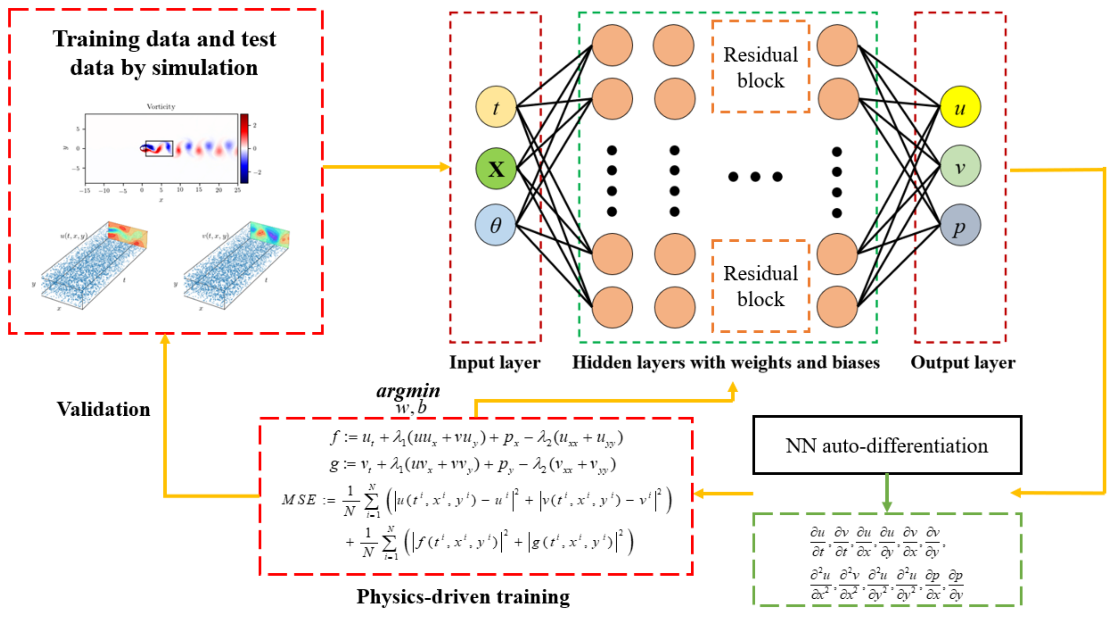
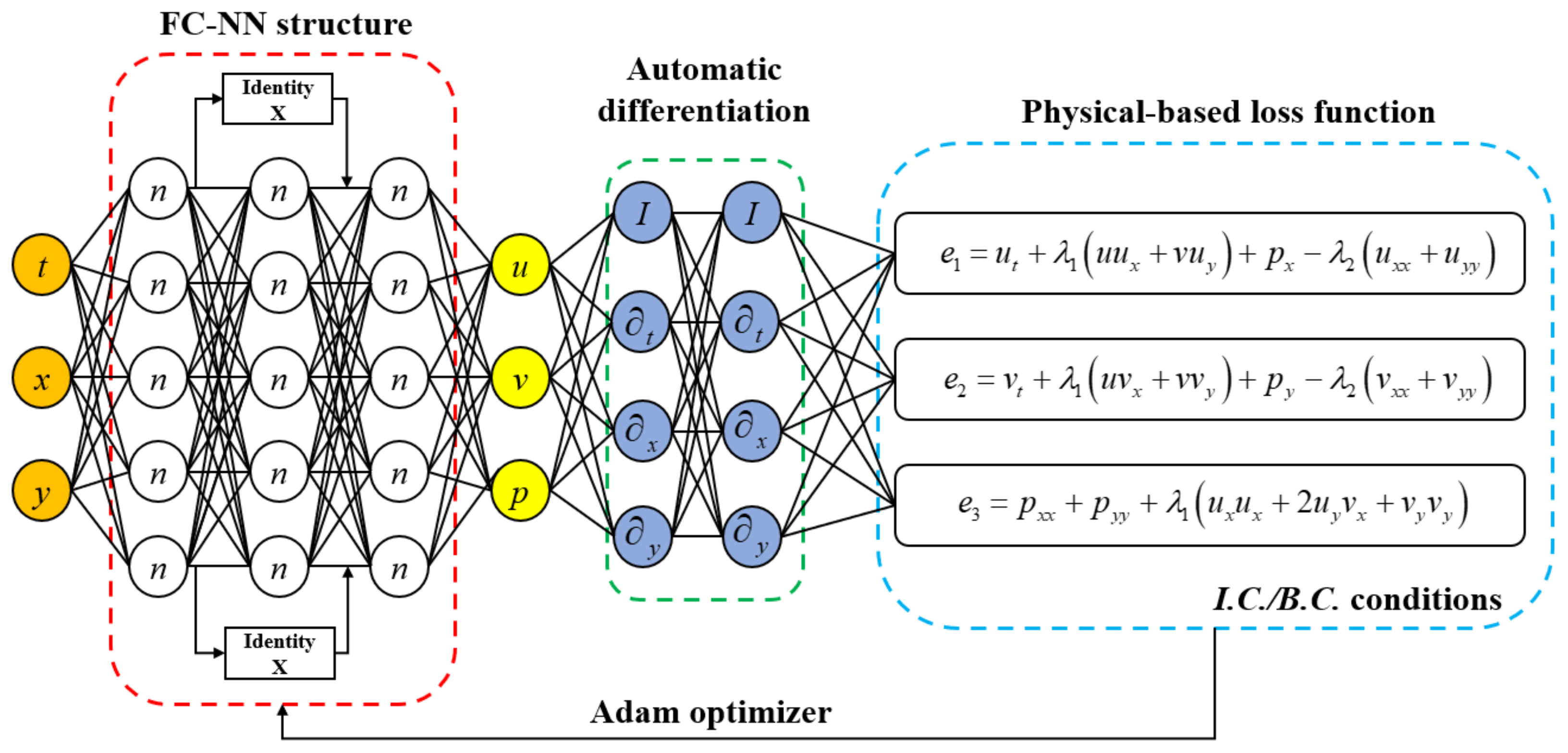
The aim of this paper is to propose a physics informed neural network combined with Resnet blocks (Res-PINN) to solve the fluid dynamics problems based on Burger’s equations and Naiver-Stokes equations. The fully-connected neural network (FC-NN) is designed to solve the information of the fluid flows. The examples of cavity flow and flow past cylinder are demonstrated to validate the effectiveness of the Res-PINN. This method can predict the fluid dynamics according to the physics-constrained conditions and initial/boundary conditions. In this paper, the novelty of the work is to embed the physical law into the loss function which can reduce the amount the training data. In addition, the physics informed neural network can solve the inverse problems of the fluid dynamics. A schematic diagram of the physics informed neural network for solving the model of the fluid dynamics can be described in Figure 1. Resnet block is applied to make the neural network more stable. The Xavier initialization method is applied to decide the initial weights and biases which can improve the convergence speed. The auto-differential technique is utilized to calculate the gradients and the governing equations are embedded into the loss function. The training set is 60% of the whole dataset while the validation set is 40% of the whole dataset. The flow information in the last moment are selected in the validation set.

The structure of this paper can be viewed as follows. Section 2 introduces the method of the Res-PINN and compared to the traditional deep learning method for fluid dynamics problems. In Section 3, the optimal methods, Xavier initialization and Adam optimizer, are adopted to optimize the Res-PINN, the swish activation function with the adjustable parameter is also utilized to ensure the effectiveness of approach. Section 4 firstly solve the Burger’s equation with discontinuous solutions to testifies the wide adaptability of the method. Then the cavity flow and flow past cylinder based on N-S equations are solved and discussed. Section 5 concludes all work in this paper.

2. Methodology

2.1. Overview

Most fluid flows, such as cavity flow, pipeline flow and flow past bluff body, can be represented by the incompressible Navier-Stokes equation and can be described as follows [25]:

$$\mathcal{F}\left(u,p\right)=0\Rightarrow \left\{\begin{array}{cc}\nabla \cdot u_{}=0\hfill & x,t\in {\Omega }_{f,t},\theta \in {ℝ}^d\\ \frac{\partial u}{\partial t}+\left(u\cdot \nabla \right)u+\frac{1}{\rho }\nabla p-\nu {\nabla }^{2}u+b_f=0,& x,t\in {\Omega }_{f,t},\theta \in {ℝ}^d\end{array}\right.$$

(1)

where u denotes the velocity field (including streamwise velocity and crosswise velocity); p the pressure field; $\rho$ and $\nu$ the density and viscosity of the fluid, respectively; b_f the body force; Ω_f,t denotes the spatial-temporal domain; $\theta$ denotes the parameters in the N-S equations such as the information of boundary conditions, the properties of fluid and the value of the domains, etc. The unique solution under different statements is constrained by the initial conditions and boundary conditions and can be described as follows:

$$\begin{array}{ll}\mathcal{I}\left(x,p,u,\theta \right)=0,& x\in {\Omega }_f,t=0,\theta \in {ℝ}^d\\ \mathcal{B}\left(t,x,p,u,\theta \right)=0,& x,t\in \partial {\Omega }_f\times \left[0,T\right],\theta \in {ℝ}^d\end{array}$$

(2)

where $\mathcal{I}$ and $\mathcal{B}$ are the differential operators of the initial and boundary conditions, respectively. When parameters $\theta$ are determined, the solution of the flow dynamics (i.e., $u(t,x)$ and $p\left(t,x\right)$) can be obatined numerically by discretizing the Equations (1) and (2) utilizing the finite difference/finite volume/finite element methods. However, this approach needs to generate large numbers of mesh and calculate the nonlinear problems iteratively which itself is time-consuming. In addition, some parameters in the fluid dynamics is difficult to be confirmed. The generation of computational meshes is a challenge when solving for the complex configuration in the numerical simulation.

To enable rapid and efficient calculations in accordance with the forward/inverse uncertainty quantification and optimization modes, a deep learning method based on PINN, which is built up by the FC-NN strucutre, is constructured to calculate the fluid informations according to Naiver-Stokes equations. The data sample can be obtained by the numerical simulations or experiments. Then the input layer include time t, spatial coordinates x, and the parameters of fluid $\theta$ while the output layer composes velocity and pressure field. The hidden layer including many layers is able to solve the nonlinearity. The auto-differentiation technique is utilized to obtain the differential variables in the N-S equations and then are embedded into loss function. The loss funtion and initial/boundary conditions are trained by the optimizal method to reach to minimum and then solution of the N-S function can be achieved.

2.2. Deep Neural Network and Physical Informed Neural Network

Artificial neural network (ANN) has been a research hotspot in the field of artificial intelligence since 1980s. It abstracts the neural network of human brain from the perspective of information processing, establishes some simple model, and forms different networks according to different connection modes. Mathematically, ANN can be described as a direct graph which is composed of a group of vertices representing neurons and a group of edges representing links. There are many variants of the neural network, such as FC-NN, CNN and recurrent neural network (RNN), etc., to perform various increasingly complex tasks [26]. In this paper, the feedforward neural network, which is also referred to as a multilayer perceptron (MLP), is adopted to solve the problem. A FC-NN structure can be described by:

$$z_l=f_l\left(W_l^T{z}_{l-1}+b_l\right)$$

(3)

where $z_l$ denotes the hidden layers between the input layer and output layer; the subscript l the index of the layer; $W_l^T$ and $b_l$ are the weight matrix and bias vector, respectively; $f_l\left(·\right)$ denotes the activation function (e.g., sigmoid function, ReLU function and tanh function, etc.) which can improve nonlinear treatment capability. The velocity and pressure of the fluid flow can be calculated by the feedforward algorithm as Equation (3). Since only weight matrixes and bias vectors are considered to be trained, the computational cost of the FC-NN can be neglected compared to that of traditional numerical simulations.

Conventionally, the deep learning method is for solving fluid dynamics problems by building up input and output relations. The solution can be calculated by a black-box surrogate model, such as fully-connected neural network (FC-NN) and convolutional neural network (CNN), the process can be demonstrated as:

$$f\left(t,x,\theta \right)\approx \tilde{f}\left(t,x,\theta \right)\triangleq z_l\left(t,x,\theta ;W,b\right)$$

(4)

where $f(t,x,\theta )$ denotes the exact solution of the fluid dynamics including veloctiy field and pressure field; $z_l(t,x,\theta ,W,b)$ the structure of neural network; $\tilde{f}(t,x,\theta )$ the local minimized trained by the FC-NN. The loss function can be formulated:

$$\begin{array}{l}{\mathcal{L}}_{data}(W,b)=\frac{1}{N}{\left|f^d\left(t,x,\theta \right)-z_l\left(t,x,\theta ;W,b\right)\right|}^2\\ \hfill W^{\ast },b^{\ast }=\underset{w,b}{argmin}{\mathcal{L}}_{data}(W,b)\hfill \end{array}$$

(5)

where ${\mathcal{L}}_{data}\left(W,b\right)$ represent the loss function which is defined as ‘data-based loss’ by Sun et al. (2020) [27]; $W^{\ast }$ and $b^{\ast }$ denote the weights and biases trained by the optimization; $f^d\left(t,x,\theta \right)$ the training data.

However, the traditional surrogate model mentioned above is a black-box model which requires large number of training samples to build up a input-output relationship. Moreover, the black-box model is absence of the physical interpretability, it means that the predicting unknown data is not convincing enough. Therefore, the physical informed neural network (PINN) is proposed in this paper. The structure of the loss function by PINN method can be defined as follow:

$$\begin{array}{cc}\hfill {\mathcal{L}}_{phy}(\mathbf{W},\mathbf{b})& =\underset{\underset{Initial/Boundary conditions}{⏟}}{\frac{1}{N_u}\sum _{i=1}^{N_u}{\left|\mathbf{u}\left(t_{\mathbf{u}}^i,x_{\mathbf{u}}^i\right)-{\mathbf{u}}^i\right|}^2}+\underset{\underset{Structure imposed by N-S equations}{⏟}}{\frac{1}{N_f}\sum _{i=1}^{N_f}{\left|\frac{\partial \mathbf{u}}{\partial t}+\left(\mathbf{u}·\nabla \right)\mathbf{u}+\frac{1}{\rho }\nabla p-\nu {\nabla }^2\mathbf{u}+{\mathbf{b}}_f\right|}^2}\hfill \\ & \underset{\underset{Mass conservation}{⏟}}{+\frac{1}{N_f}\sum _{i=1}^{N_f}{\left|\nabla \mathbf{u}\right|}^2}\hfill \\ & {\mathbf{W}}^{*},{\mathbf{b}}^{*}=\underset{\mathbf{w},\mathbf{b}}{argmin} {\mathcal{L}}_{phy}(\mathbf{W},\mathbf{b})\hfill \end{array}$$

(6)

The N-S equations, Mass conservation equation and boundary condition are embedded into the loss function. The first and second derivative terms of velocity and pressure are calculated directly by automatic differentiation. It is worth emphasizing that automatic differentiation is a method between symbolic differentiation and numerical differentiation. Numerical differentiation emphasizes directly substituting into numerical approximate solution at the beginning while symbolic differentiation emphasizes solving algebra directly before substituting numerical. Automatic differentiation applies symbolic differentiation to the most basic operators, such as constant, power function, exponential function, logarithmic function, trigonometric function, etc., and then substituting it into the numerical value, retaining the intermediate result, and finally applying it to the whole function. Therefore, the automatic differentiation can avoid truncation and round-off errors effectively [28]. In this paper, the automatic differentiation technique is carried out by the Pytorch framework. The Adam algorithm is adopted to optimize the loss function and the more information on this method is introduced in Section 3.2.

2.3. Residual Neural Network (Resnet)

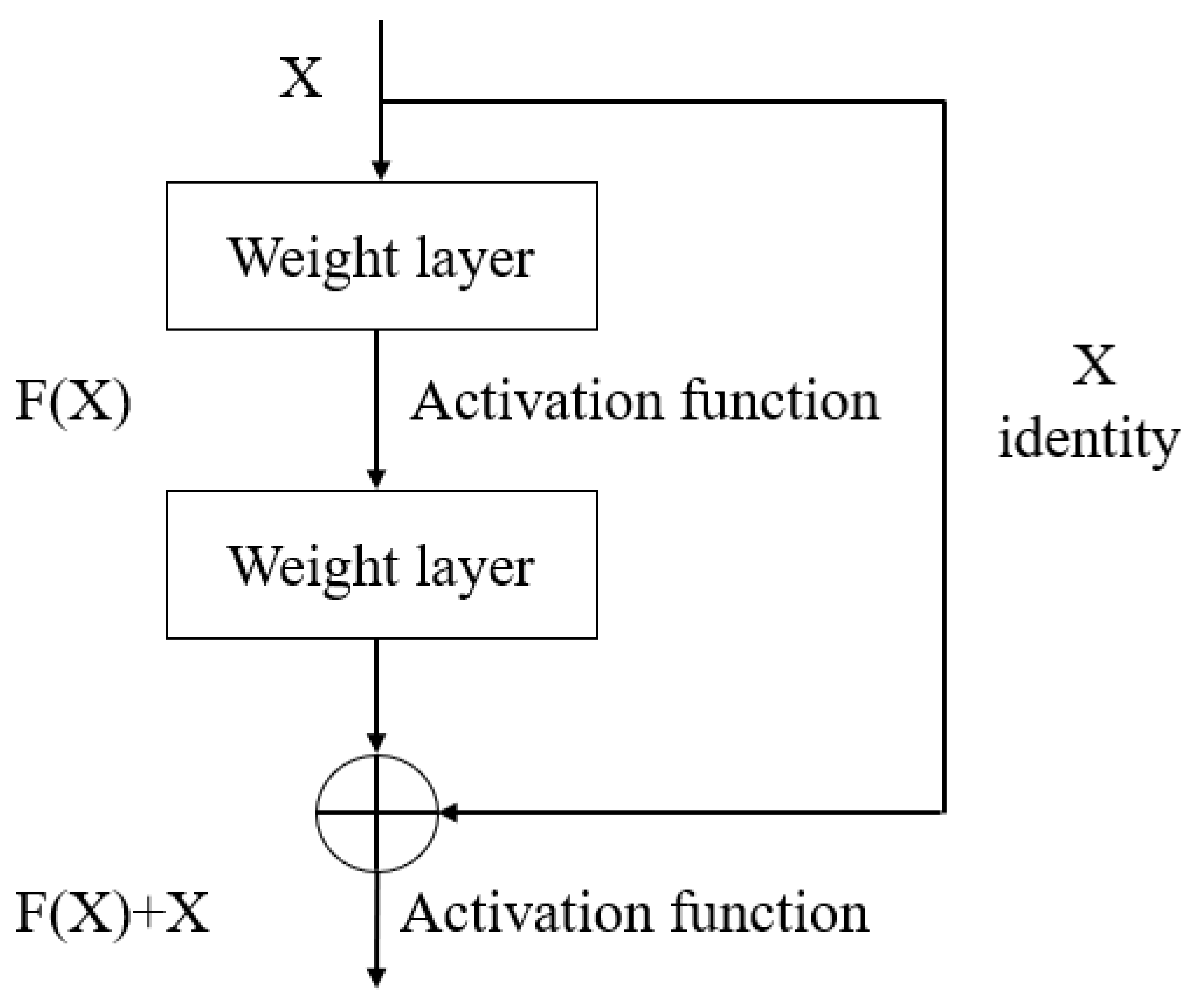
The structure of the deep neural network can convert into a shallow neural network if the hidden layers are identity mays. Therefore, the problem is transformed to learn the identity mapping. In fact, the existing neural networks are difficult to fit the potential identity mapping function $H(x)=x$. However, if the neural network is designed as $H(x)=F(x)+x$ and the identity mapping is directly regarded as a part of the network. The problem can be transformed into learning a residual function: $F(x)=H(x)-x$. As long as $F(x)=0$, an identity mapping $H(x)=x$ is generated. Moreover, training residuals can reduce the complexity of solving problems instead of training mapping identity.

He et al. (2015) adopted residual machine learning to every few hidden layers [25]. A building block can be shown in Figure 2. Mathematically, a building block can be demonstrated as the following equation:

$$y=F\left(x,\left\{W_i\right\}\right)+x$$

(7)

where $x,y$ denotes input and output values, respectively; the function $F(x,\left\{W_i\right\})$ is the residual mapping to be trained.

In addition, the right line in Figure 2 is called a shortcut connection. By jumping in front of the activation function, the output from before layer or several layers is added with the current layer and is injected to the activation function which is as the output from the current layer. Moreover, the residual part in Figure 2 can be expressed as follows:

$$F=W_2\sigma \left(W_{1}x\right)$$

(8)

3. Structural Optimization

3.1. Model Parameter Initialization Method

When the form of the partial differential equation is cast by Res-PINN and the fully-connected neural network with residual blocks are determined. In order to make the information flow better in the network, the output variance of each layer should be as equal as possible. Therefore, the initial weights in each layer should meet certain conditions. designed Xavier method is designed to solve this problem [29].

The output in one layer can be calculated as follows:

$$y=w_1{x}_1+\cdots +w_{n_i}{x}_x+b$$

(9)

According to the knowledge of probability and statistics, the following variance formula can be deduced as follows:

$$Var(w_i{x}_i)=E{\left[w_i\right]}^{2}Var(x_i)+E{\left[x_i\right]}^{2}Var(w_i)+Var(w_i)Var(x_i)$$

(10)

We can assume the average values of input and weights are zero, the Equation (13) can be simplified as:

$$Var(w_i{x}_i)=Var(w_i)Var(x_i)$$

(11)

It is further assumed that input and weights are independent identically distributed, the problem can be described:

$$Var(y)=n_{i}Var(w_i)Var(x_i)$$

(12)

To ensure that the input and output variances are consistent, it can be deduced as follow:

$$Var(w_i)=\frac{1}{n_i}$$

(13)

For a multi-layer network, the variance of a layer can be expressed in the form of accumulation:

$$Var[z^i]=Var[x]{\displaystyle \prod _{i^{\prime }=0}^{i-1}{n}_i^{\prime }}Var[w^{i^{\prime }}]$$

(14)

When calculate the gradients, the back propagation has the same form:

$$Var[\frac{\partial Cost}{\partial s^i}]=Var[\frac{\partial Cost}{\partial s^d}]{\displaystyle \prod _{i^{\prime }=i}^d{n}_{i^{\prime }+1}Var[w^{i^{\prime }}]}$$

(15)

Therefore, in order to ensure that the variance of each layer is consistent in forward and backward propagation, the initial weights need to meet the below conditions:

$$\begin{array}{lll}\forall i,& & n_{i}Var\left[w^i\right]=1\hfill \\ \forall i,& & n_{i+1}Var\left[w^i\right]=1\end{array}$$

(16)

The Xavier initialization is the following uniform distribution:

$$w\sim U\left[-\frac{\sqrt{6}}{\sqrt{n_j+n_{j+1}}},\frac{\sqrt{6}}{\sqrt{n_j+n_{j+1}}}\right]$$

(17)

3.2. Adam Optimization

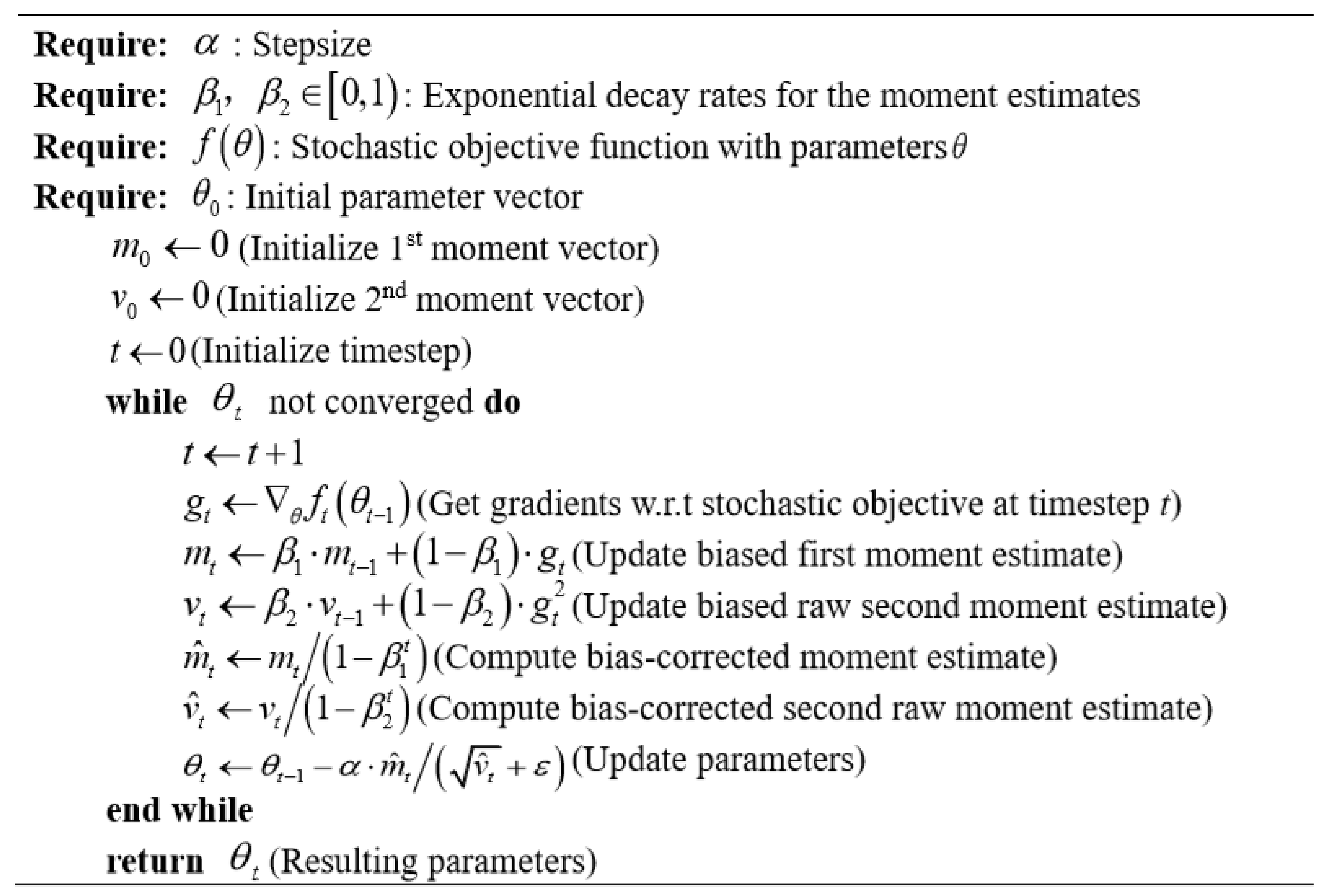
In order to reduce the error of the loss function, the Adam optimizer is utilized to optimize the target function. Adam algorithm is different from traditional random gradient descent. Adam optimizer can constantly adjust the learning rates with the situation changes in the learning process. Furthermore, another advantage of the Adam optimizer can change the learning rate through the average of the nearest weight gradient, it means that the algorithm has a good performance in non-stationary problem.

The step of the Adam optimizer can be described as follows:

• Step 1: compute gradients of parameters at time step w.r.t stochastic objective functions;
• Step 2: compute first moment estimate, to help avoid disordered moving, and to prevent settling into local optima;
• Step 3: estimate second moment estimate, to guarantee an upper bound of step size;
• Step 4: compute unbiased estimate of first moment estimate and second moment estimate;
• Step 5: update parameters.

The pseudo-code of the Adam optimization method can be viewed in Figure 3.

4. Discussion

4.1. Problem Setup

In this section, three scenarios are proposed to validate the Res-PINN’s performance on solving the fluid flow problems. First scenario is to handle the Burger’s equation with the discontinuous solutions while the last scenarios are to calculate the N-S equations with the smooth and continuous solutions including cavity flow and the unsteady flow past cylinder.

The data of the Burger’s equation is obtained by the finite element method (FEM) while that of the N-S equation is obtained by the direct numerical simulation (DNS). The fully-connected neural network is adopted to build up the Res-PINN and the Swish activation function is selected to determine the nonlinear capacity. It is noteworthy that the Swish activation function has a better performance in improving the convergence rate and accuracy of the neural network. The value of learning rate is dynamic and the initial value is 0.001. The uncertainties in the fluid properties and flow information are solved by the Res-PINN. In this study, only steady-state of fluid flows are selected for proof-of-concept. Accordingly, the initial conditions can be neglected.

The Res-PINN is implemented in the PyTorch platform. The perfect structure of the deep neural network, including number of layers, number of neurons per layer, is not fully understood that need to be tested by the trail and error. In addition, the different number of training samples are also selected to validate that the Res-PINN has an accurate performance in solving fluid flows problems based on finite data samples.

4.2. PINN Method for Burger’s Equation with Discontinuous Solution

The incompressible fluid relevant to cavity flow and flow past cylinder are considered in this section. It is noteworthy that the mentioned above flow solutions are almost smooth and continuous. Therefore, the burger’s equation, as a canonical problem with discontinuous solution, is proposed to demonstrate the physical informed neural network can also has a good performance in solving discontinuous problems. The Burger’s equation with the initial and boundary conditions can be described as follow:

$$\begin{array}{lll}{u}_t+u{u}_x-(0.01/\pi )u_{xx}=0,& x\in \left[1,1\right],& t\in \left[0,1\right],\\ u\left(0,x\right)=-sin\left(\pi x\right),& & \\ u\left(t,-1\right)=u\left(t,1\right)=0& & \end{array}$$

(18)

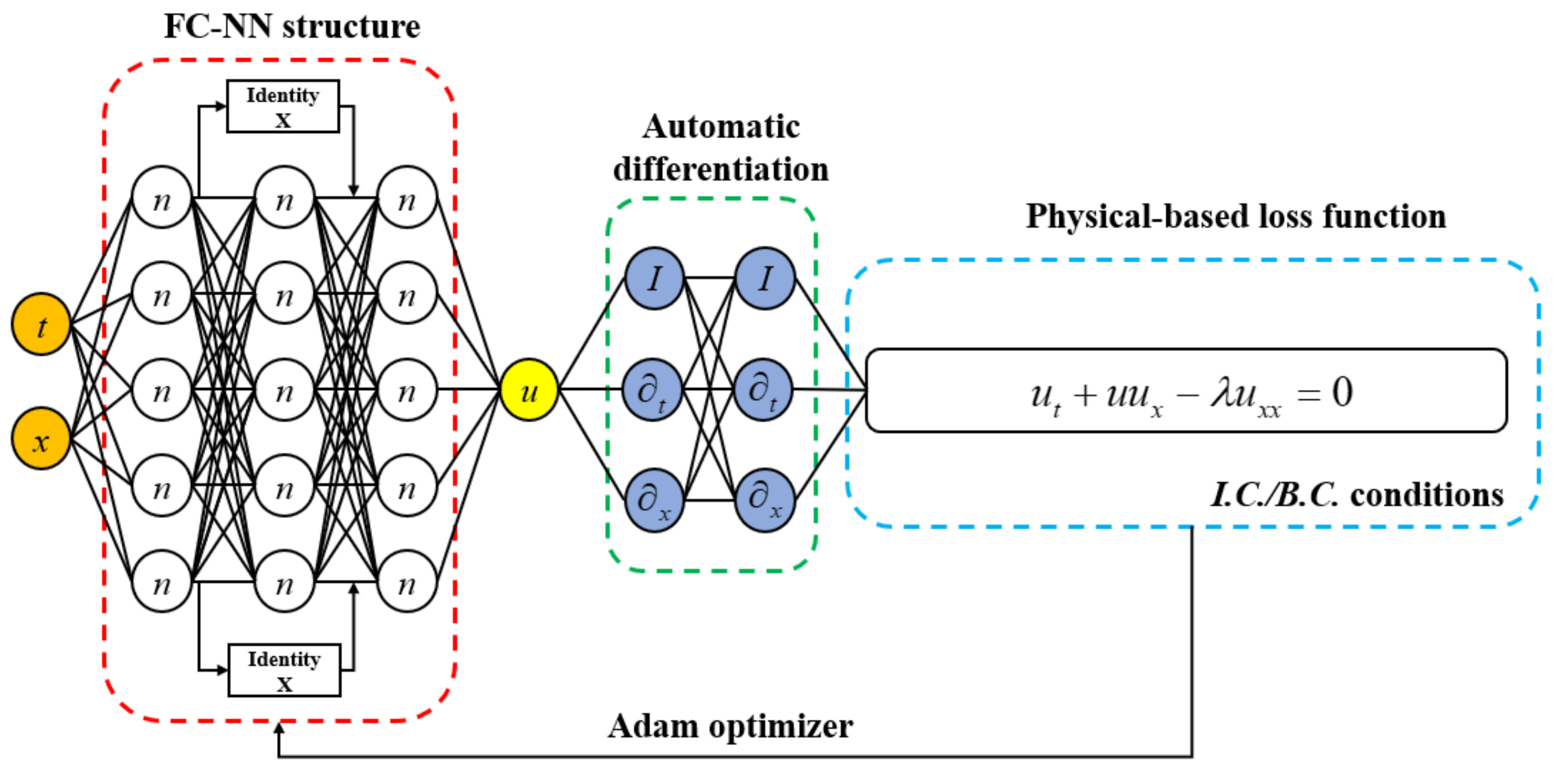
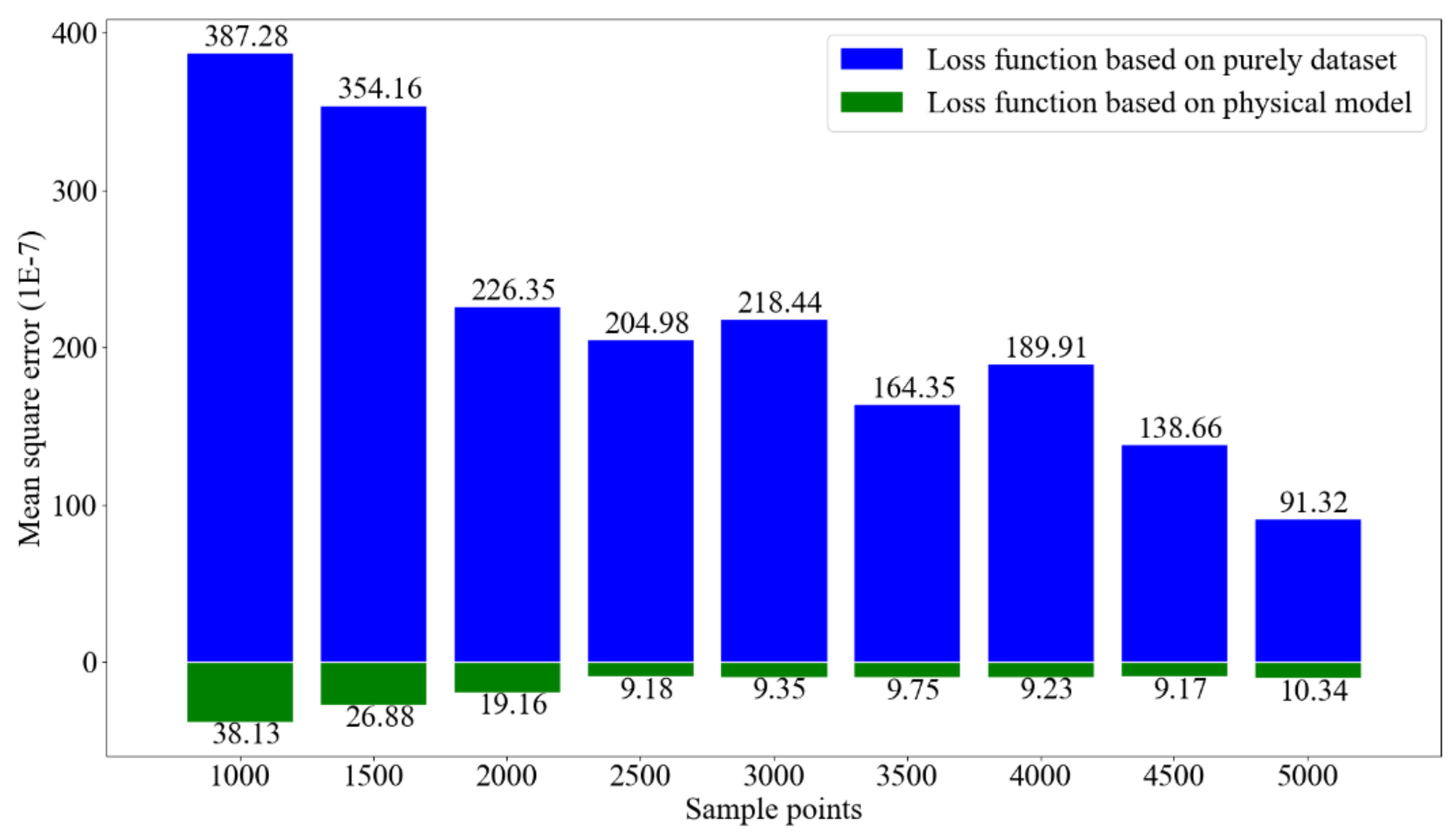
The process of Res-PINN solving the burger’s equations can be viewed in Figure 4. The time t and spatial coordinates x are selected as input while the velocity u is seemed as output and the layers and neurons in each layer between input and output which consist the FC-NN structure. For illustration purpose only, the structure of network including 3 hidden layers and 5 neurons per hidden layer are demonstrated in Figure 4. The automatic differentiation technique is adopted to compute the physical-based loss function and the velocity u on the training data is calculated by minimizing the loss function. In addition, I in the green box denotes the identity operator while the ${\partial }_t$ differential operator which can be explained as activation operator. In addition, the term does not in the physical-based loss function (e.g., $u_{tt}$ or $u_{tx}$) which coefficients are set to be zero. To determine the best structure of the Res-PINN, mean square value of the latent solution under the different layers and different neurons in each layer are demonstrated in

Table 1. The mean square error between predict value and exact value in validation set with different layers and neurons.

	Neurons	10	20	30	40
Layers
2 (without Restnet)		$3.8\times {10}^{-3}$	$2.1\times {10}^{-3}$	$6.6\times {10}^{-4}$	$8.7\times {10}^{-3}$
4		$1.3\times {10}^{-4}$	$8.8\times {10}^{-5}$	$6.7\times {10}^{-6}$	$6.4\times {10}^{-6}$
6		$8.2\times {10}^{-5}$	$5.3\times {10}^{-5}$	$4.3\times {10}^{-6}$	$6.1\times {10}^{-6}$
8		$6.6\times {10}^{-5}$	$7.2\times {10}^{-6}$	$2.4\times {10}^{-6}$	$7.2\times {10}^{-6}$
10		$2.3\times {10}^{-6}$	$9.2\times {10}^{-7}$	$8.2\times {10}^{-6}$	$6.7\times {10}^{-6}$

. It can be demonstrated that the best structure of the Res-PINN includes 10 hidden layers with 20 neurons in each layer. The more complex structure of the neural network does not mean that the Res-PINN has the higher performance in solving Burger’s equation, it may result in over-fitting and bad generalization ability. Furthermore, the comparisons between loss function based on purely dataset and loss function based on physical model can be demonstrated in Figure 5. The structure of 10 hidden layers with 20 neurons per layer is adopted and the different data samples to test the performance of Res-PINN and traditional deep learning. It is obvious that Res-PINN method, compared to the traditional deep learning method based on purely data, has more accurate predictions in solving Burger’s equations under limited amount of data. It demonstrates that the mean square error is pretty low when the number of training data reach to 2000. Therefore, the Res-PINN can well calculate the predict values in limited dataset and reduce the time cost.

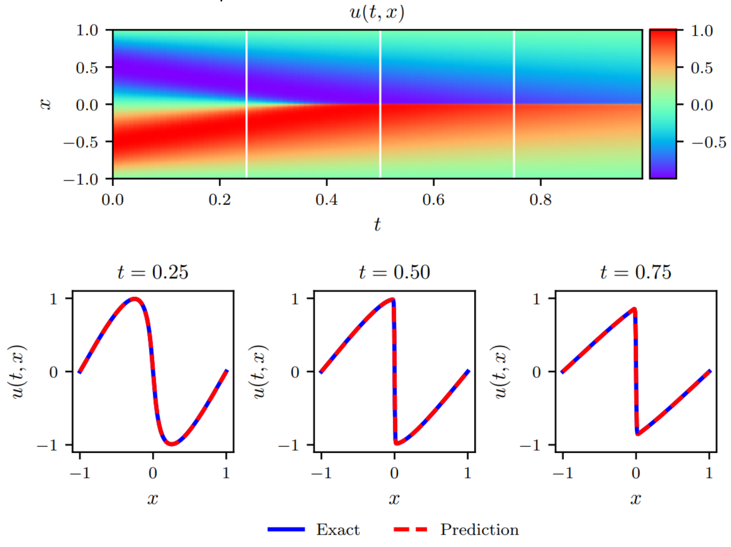
The analytical solution is compared with the solution calculated by the Res-PINN which can be viewed in Figure 6. The top of the Figure 6 is the spatial-temporal values of the Burger’s equation predicted by the analytical solution. The bottom of three figures is comparisons between predicted values (red dotted line) and exact values (blue line) at different times. It is obvious that the predicted values are almost agreement with the exact values. The mean square error of the validation set is to reach to $9.2\times {10}^{-7}$. In addition, the inverse problem of the Burger’s equation is also considered and the parameter predicted by the Res-PINN in Burger’s equation is 0.00318 which is versus with the exact parameter ($0.01/\pi$), the error is almost negligible.

4.3. Res-PINN Method for N-S Equation with Continuous Solution

In this section, the cavity flow and incompressible flow past cylinder are considered to identify the N-S equations. Cavity flow refers to the flow of closed incompressible fluid (such as water) driven by the top plate at a constant speed in a regular area. Almost all flow phenomena that may occur in incompressible fluid can be observed in square cavity flow. The cavity flow can be described based on dimensionless N-S equation as follow:

$$\begin{array}{l}{u}_t+(u{u}_x+v{u}_y)=-p_x+R{e}^{-1}\left(u_{xx}+u_{yy}\right)\\ v_t+(u{v}_x+v{v}_x)=-p_y+R{e}^{-1}\left(v_{xx}+v_{yy}\right)\\ p_{xx}+p_{yy}=-(u_x{u}_x+2u_y{v}_x+v_y{v}_y)\end{array}$$

(19)

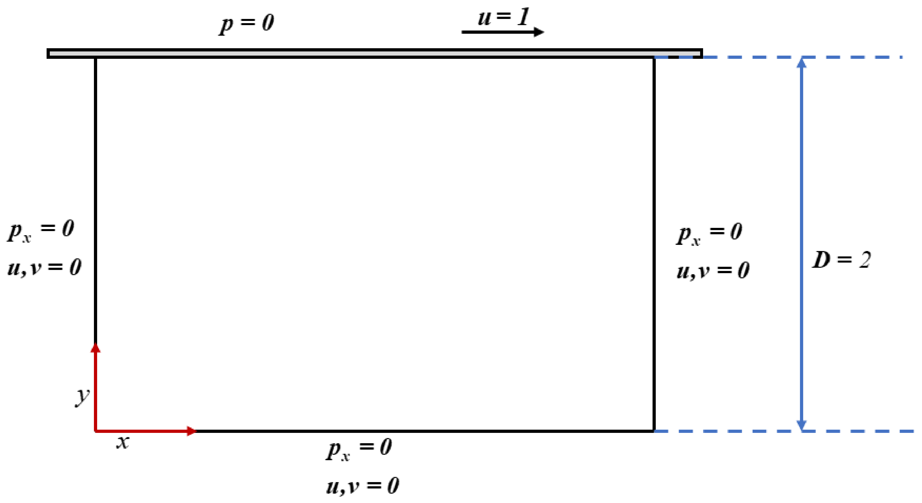
where $Re$ denotes the Reynolds number. u and v represent the x-direction and y-direction of the velocity flied, respectively; p the pressure field. The scenario of the 2-D cavity flow and the boundary conditions can be viewed in Figure 7. The boundary conditions of the top cover, pressure is zero and x-direction velocity is 1, while that of the other three boundaries, the first derivative of pressure in x direction is zero and two direction velocities are also zero.

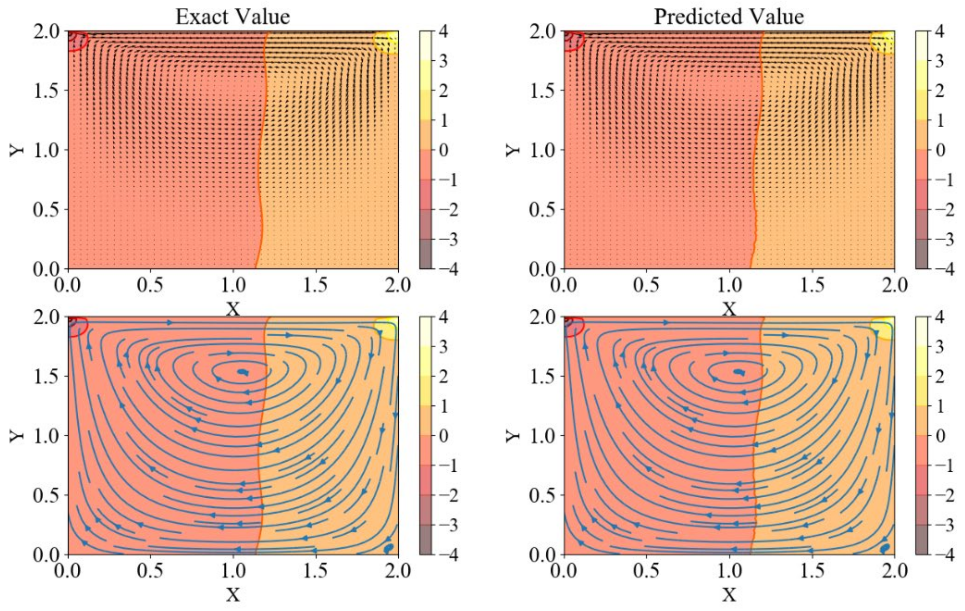
Uniform sampling method is utilized to obtain the training data and different samples are chosen to train the model. Before t = 1, the training samples are obtained per 0.1 as a frame and the test samples are selected at t = 1. The process of the calculation can be demonstrated in Figure 8. The time and space coordinates are viewed as input while pressure and velocity are seemed as output. To further investigate the Res-PINN’s accuracy, the parameters like Re are viewed as unknown parameter $\left({\lambda }_1,{\lambda }_2\right)$ in loss function. The true values of parameters are 1 and 20. The 8 hidden layers with 20 neurons each layer are selected to construct the FC-NN structure and 400 samples per frame are obtained to calculate the N-S equations. The predicted values can be viewed in Figure 9. Left two panels are exact flow field while right two panels are predicted flow field. It is obvious that the Res-PINN has a good performance in predicting the velocity and pressure. The mean square error of flow field can be viewed in

Table 2. The mean square error between predict value and exact value in cavity flow.

	Mean Square Error (Training Set)	Mean Square Error (Validation Set)
$u$	$2.1\times {10}^{-7}$	$4.1\times {10}^{-6}$
$v$	$5.2\times {10}^{-7}$	$9.8\times {10}^{-7}$
$p$	$1.3\times {10}^{-5}$	$3.2\times {10}^{-3}$

. In addition, the predicted parameters of ${\lambda }_1$ and ${\lambda }_2$ are 1 and 19.973 which are almost same with the exact values.

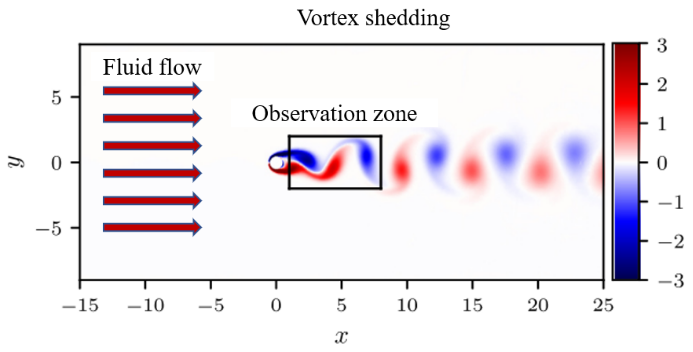
A classical problem of fluid-structure interaction which can also be described by Navier-Stokes equation is proposed to verify the Res-PINN method. In Figure 10, the incompressible flow around a circular cylinder with dynamic vortex shedding is demonstrated. It can be assumed that the inlet condition is the free stream velocity while the outlet condition is free pressure zone. The slide wall boundary conditions are imposed on the two sides of the flow filed. The non-dimensional inlet velocity $u=1$, cylinder diameter $D=1$, and kinematic viscosity $\nu =0.01$. The direct numerical simulation (DNS) is adopted to calculate the N-S equation and generate the dataset [30]. The black box behind the cylinder is the data collection and that is utilized to calculate the N-S equations. The form of 2-D Navier-Stokes equation can be described explicitly as follow:

$$\begin{array}{l}{u}_t+(u{u}_x+v{u}_y)=-p_x+R{e}^{-1}(u_{xx}+u_{yy}),\\ v_t+(u{v}_x+v{v}_y)=-p_y+R{e}^{-1}(v_{xx}+v_{yy})\\ u_x+u_y=0\end{array}$$

(20)

where $u(t,x,y)$ means the x-direction of the velocity field, $v(t,x,y)$ the y-direction of the velocity field, $p(t,x,y)$ the pressure in the flow field. It can be assumed as: $u={\psi }_x,v=-{\psi }_y$ which can meet the continuity equation automatically.

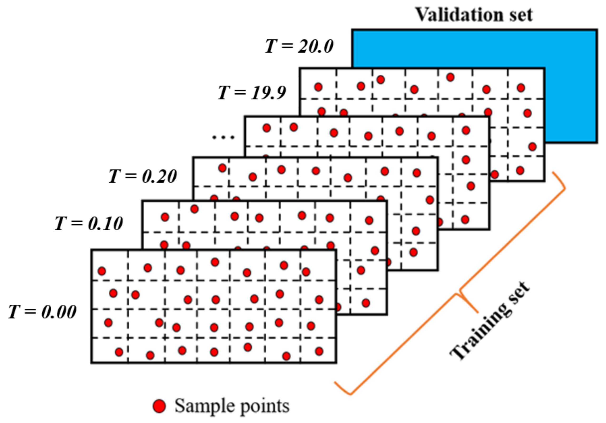
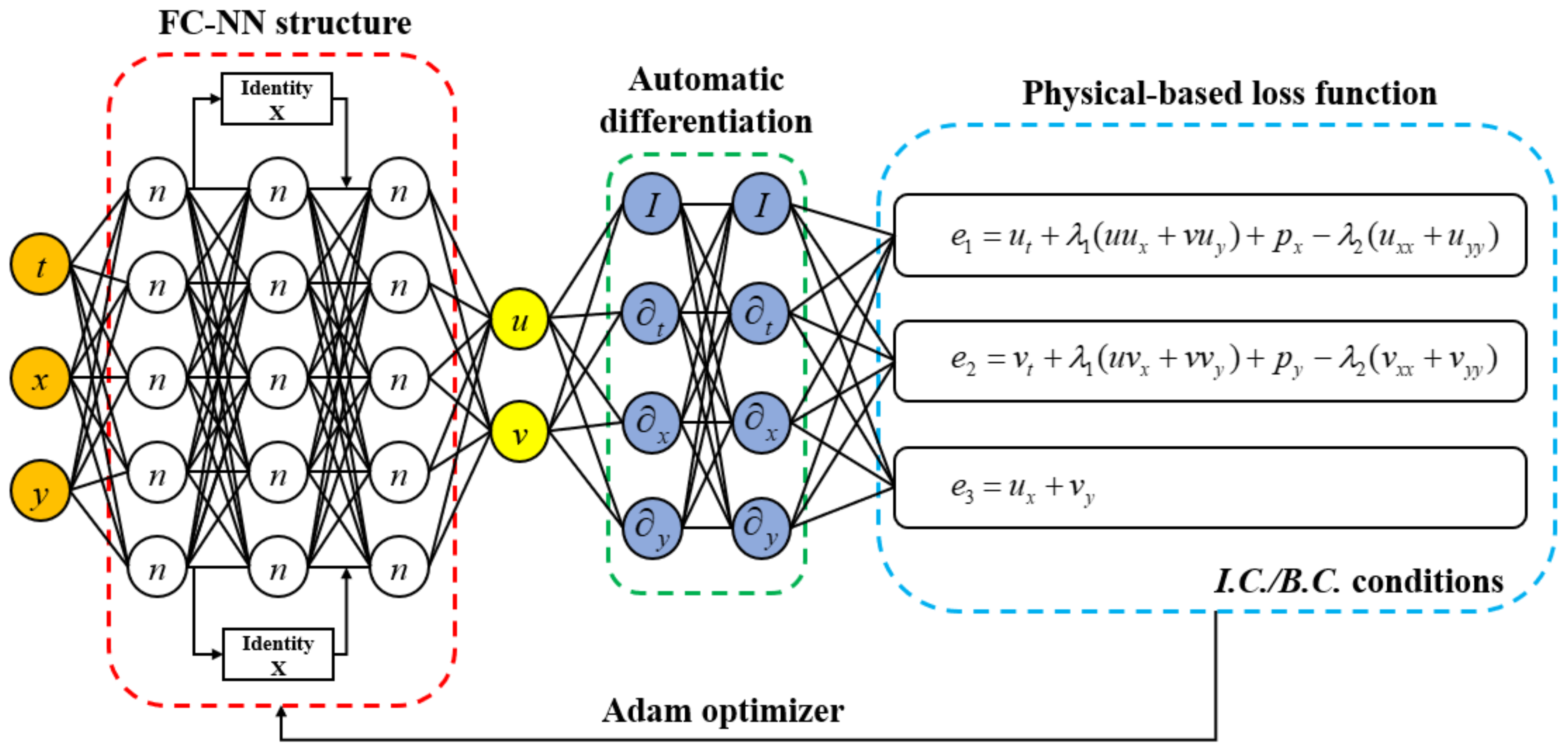
In this section, Latin hypercube sampling (LHS) is selected to obtain the training set. LHS is a kind of approximate random sampling method from multivariate parameter distribution. It belongs to stratified sampling technology and is often used in computer experiments or Monte Carlo integration. The training data is obtained from T = 0.0 to T = 19.9 with 0.1 interval while the validation data is obtained at T = 20. The specific sampling method is shown in Figure 11. The time and space coordinates are selected as input and the velocities are selected as output. In this example, the pressure is seemed as an unknown value that need to be identified. What’s more, the unknown parameters, non-dimension coefficients, are also calculated to validate the performance the Res-PINN. The physical-based loss functions include the conservation equation and N-S equations are gradient computed by Adam optimizer. The structure of neural network is 9 hidden layers with 20 neurons each layer, the Res-PINN and PINN are compared in 4000 samples. The steam-wise $u(t,x,y)$ and transverse-wise $v(t,x,y)$ velocity are also imposed by 1% uncorrelated Gaussian noise to validate that the Res-PINN proposed in this paper can also has a good performance to filter the noise. The detailed N-S equations are informed into neural network (flow past cylinder) which can be viewed in Figure 12.

A conclusion of our prediction for 2-D N-S equation and compares with the work utilized by PINN is presented in

Table 3. The Correct NS equation versus with the identified NS equation.

Correct N-S eqaution	$\begin{array}{l}{u}_t+(u{u}_x+v{u}_y)=-p_x+0.01(u_{xx}+u_{yy}),\\ v_t+(u{v}_x+v{v}_y)=-p_y+0.01(v_{xx}+v_{yy})\end{array}$
Identified N-S equation with clean data (PINN)	$\begin{array}{l}{u}_t+0.999(u{u}_x+v{u}_y)=-p_x+0.01047(u_{xx}+u_{yy}),\\ v_t+0.999(u{v}_x+v{v}_y)=-p_y+0.01047(v_{xx}+v_{yy})\end{array}$
Identified N-S equation with clean data (Res-PINN)	$\begin{array}{l}{u}_t+1.000(u{u}_x+v{u}_y)=-p_x+0.01006(u_{xx}+u_{yy}),\\ v_t+1.000(u{v}_x+v{v}_y)=-p_y+0.01006(v_{xx}+v_{yy})\end{array}$
Identified N-S equation with noise data (PINN)	$\begin{array}{l}{u}_t+0.998(u{u}_x+v{u}_y)=-p_x+0.01057(u_{xx}+u_{yy}),\\ v_t+0.998(u{v}_x+v{v}_y)=-p_y+0.01057(v_{xx}+v_{yy})\end{array}$
Identified N-S equation with noise data (Res-PINN)	$\begin{array}{l}{u}_t+1.000(u{u}_x+v{u}_y)=-p_x+0.01011(u_{xx}+u_{yy}),\\ v_t+1.000(u{v}_x+v{v}_y)=-p_y+0.01011(v_{xx}+v_{yy})\end{array}$

. It can be viewed that the Res-PINN has a strong performance to identify the N-S equations under clean data and noise data. It can be viewed that, in the case of clean training data, the error in predicting ${\lambda }_1$ and ${\lambda }_2$ is 0%, and 0.61% respectively, which compared to the 0.078%, and 4.67% calculated by PINN. Under the noise data, the identified results are also show that Res-PINN has a good ability to predict the accuracy solution of the N-S equations. When the training data are polluted with 1% uncorrelated Gaussian noise, the unknown parameters predicted by our work is 0% and 1.08%, which compared to the 0.17%, and 5.70% obtained by PINN for ${\lambda }_1$ and ${\lambda }_2$, respectively. The magnitude of mean square errors in the velocity is reach to ${10}^{-5}$.

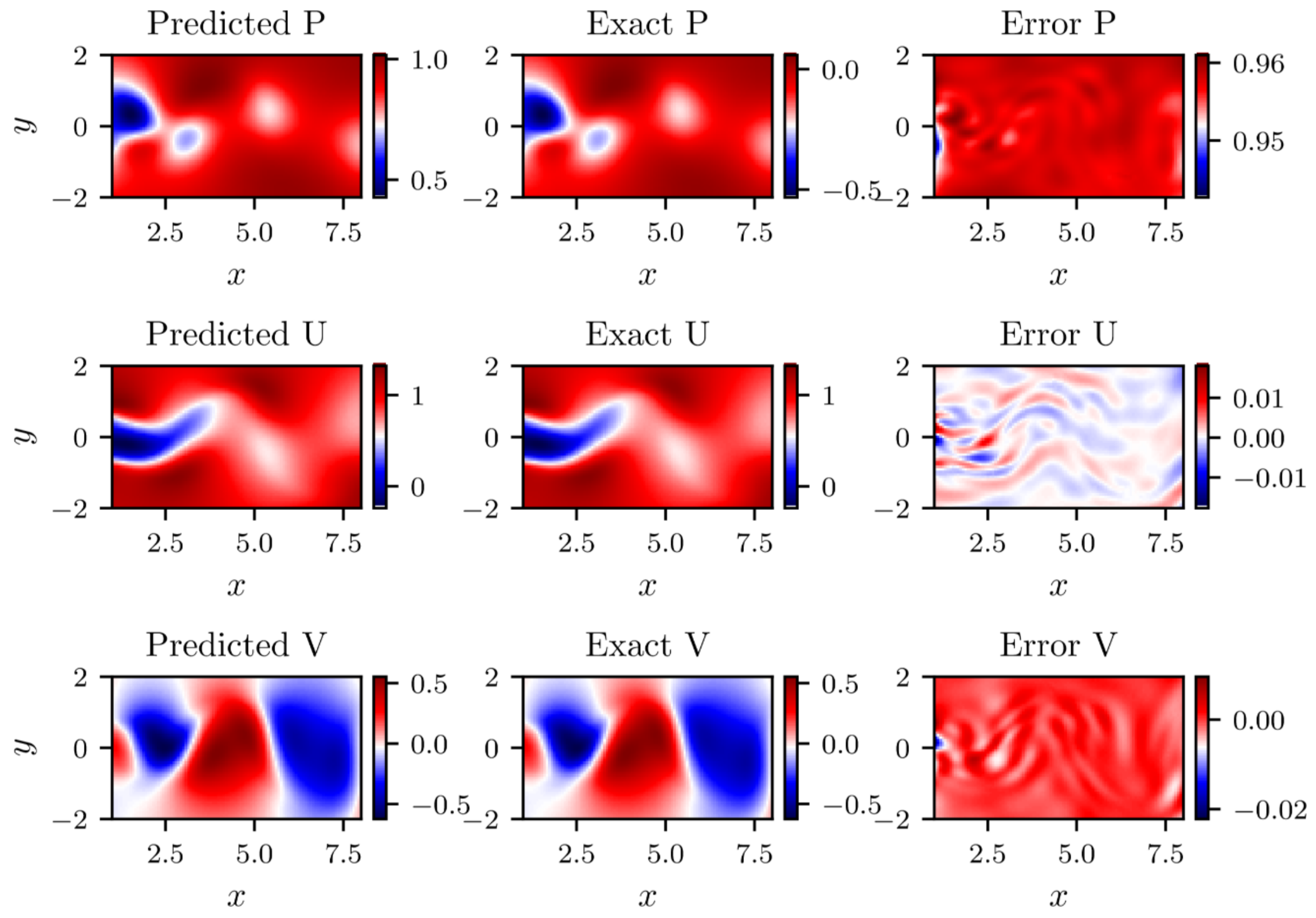
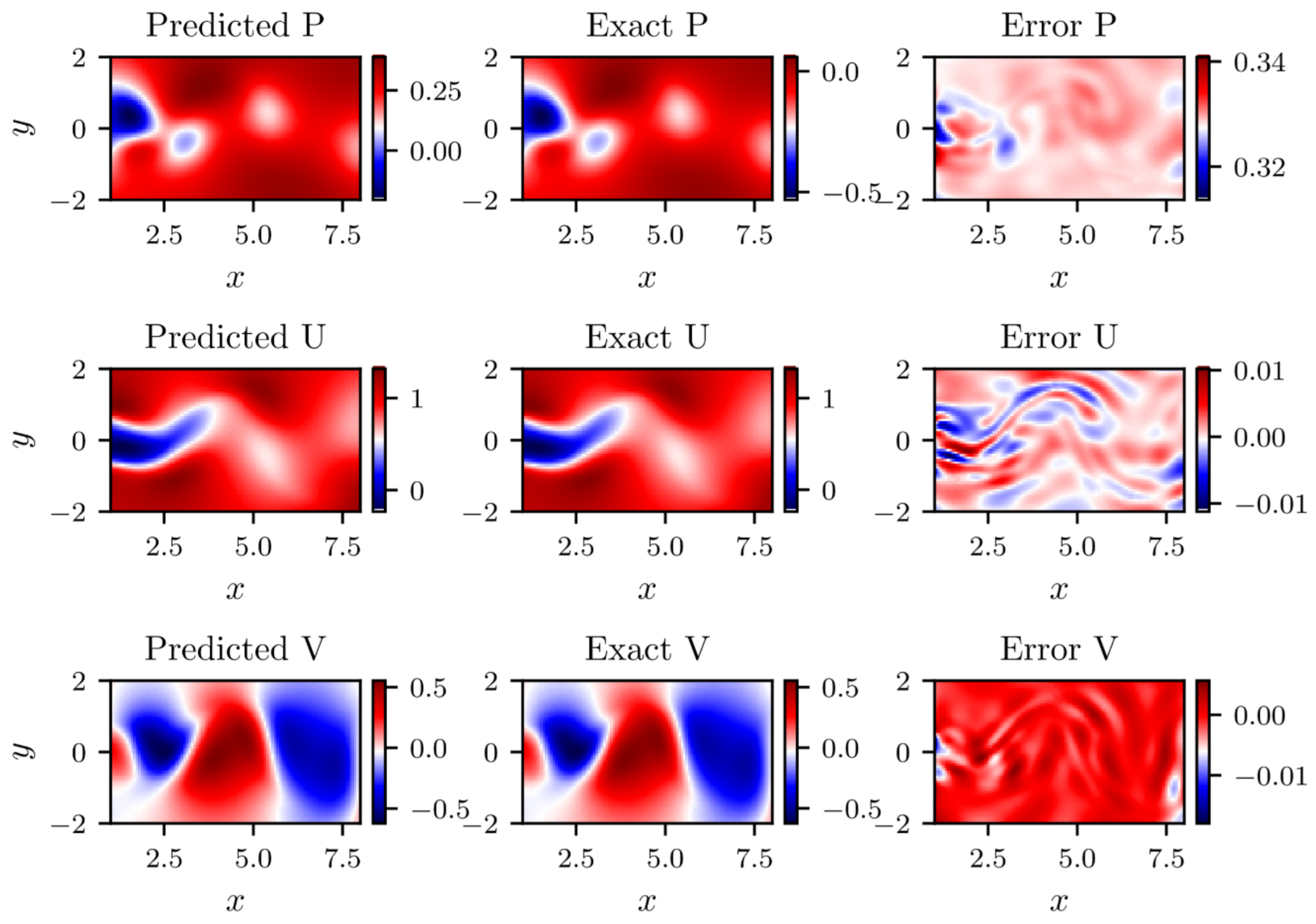
In addition, the predicted results against real instantaneous flow field at a certain time with clean data and noise data can be demonstrated in Figure 13 and Figure 14. It can be viewed that the prediction of the stream-wise velocity and transverse-wise velocity is pretty accuracy, the biggest errors in entire flow filed for stream-wise velocity and transverse-wise velocity are 0.98% and 3.1% in clean data while that are 0.99% and 3.1% in noise data, respectively. It is noteworthy that the Res-PINN also enjoys the ability to reconstruct the whole pressure field $p(t,x,y)$ although the training data on the pressure field is absent. A strange phenomenon that the difference in magnitude between the predicted pressure and exact, although the distribution of the pressure filed is almost same. It is validated by the law of the N-S equation due to the pressure field is only recognizable up to a fixed value. For the incompressible flow, the absolute value of the pressure is of no great important.

5. Conclusions

This paper firstly proposed the Res-PINN method to predict the fluid dynamics problems. Compared to the traditional deep learning method, the Res-PINN simulates the fluid flows based on physical models rather than purely data. To investigate the performance of Res-PINN, Burger’s equations and Navier-Stokes equations are selected and different scenarios (cavity flow and flow past cylinder) are adopted. The specific conclusions can be summarized as follows:

(1)

The Burger’s equation predicted by the Res-PINN and that predicted by the traditional deep learning are compared and the results show that the Res-PINN has better performance in calculating and predicting the flow fields. The Res-PINN can well predict the results under only 1000 samples.

(2)

The Navier-Stokes equations predicted by PINN and that predicted by Res-PINN are contrasted and the results demonstrate that the Res-PINN can ensure the better at accuracy. The magnitude of mean square errors of problems reach to 10⁻⁵.

(3)

the Res-PINN can well calculate the inverse parameters in partial differential equations. The errors of the inverse parameters are 0.98% and 3.1% in clean data while 0.99% and 3.1% in noisy data, it demonstrates that can well solve the inverse problem even in the noisy data.

References

- Ding, H.; Shu, C.; Yeo, K.S.; Xu, D. Simulation of incompressible vis-cous flows past a circular cylinder by hybrid FD scheme and meshless least square-based finite difference method. Comput. Methods Appl. Mech. Eng. 2004, 193, 727–744. [Google Scholar] [CrossRef]
- Liu, F.; Zheng, X.Q. A Strongly Coupled Time-Marching Method for Solving the Navier–Stokes and k-ω Turbulence Model Equations with Multigrid. J. Comput. Phys. 1996, 128, 289–300. [Google Scholar] [CrossRef] [Green Version]
- Lucia, D.J.; Beran, P.S.; Silva, W.A. Reduced-order modeling: New approached for computational physics. Prog. Aerosp. Sci. 2004, 40, 51–117. [Google Scholar] [CrossRef] [Green Version]
- Henshawa, M.J.; Badcock, K.J.; Vio, G.A. Non-linear aeroelastic prediction for aircraft applications. Prog. Aerosp. Sci. 2007, 43, 65–137. [Google Scholar] [CrossRef]
- Jovanovie, M.R.; Schmid, P.J.; Nichols, J.W. Sparsity-promoting dynamic mode decomposition. Phys. Fluids 2014, 26, 024103. [Google Scholar] [CrossRef]
- Hemati, M.S.; Williams, M.O.; Rowley, C.W. Dynamic mode decomposition for large and streaming datasets. Phys. Fluids 2014, 26, 111701. [Google Scholar] [CrossRef] [Green Version]
- Chen, G.; Li, D.; Zhou, Q. Efficient aeroelastic prediction for aircraft applications. Prog. Aerosp. Sci. 2018, 40, 51–117. [Google Scholar]
- Goodfellow, I.; Bengio, Y.; Courville, A. Deep Learning; MIT Press: Cambridge, MA, USA, 2016. [Google Scholar]
- Sainath, T.N.; Mohamed, A.; Kingsbury, B.; Ramabhadran, B. Deep convolutional neural networks for LVCSR. In Proceedings of the 2013 IEEE International Conference on Acoustics, Speech and Signal Processing (ICASSP), Vancouver, BC, Canada, 26–31 May 2013; IEEE: New York, NY, USA, 2013; pp. 8614–8618. [Google Scholar]
- Xiong, H.Y.; Alipanahi, B.; Lee, L.J.; Bretschneider, H.; Merico, D.; Yuen, R.K.; Hua, Y.; Gueroussov, S.; Najafabadi, H.S.; Hughes, T.R. The human splicing code reveals new insights into the genetic determinants of disease. Science 2015, 347, 1254806. [Google Scholar] [CrossRef] [PubMed] [Green Version]
- Ma, M.; Lu, J.; Tryggvason, G. Using statistical learning to close two-fluid multiphase flow equations for a simple bubbly system. Phys. Fluids 2015, 27, 092101. [Google Scholar] [CrossRef]
- Roshko, A. Perspectives on bluff body aerodynamics. J. Wind Eng. Ind. Aerodyn. 1993, 49, 79–100. [Google Scholar] [CrossRef]
- Ling, J.; Kurzawski, A.; Templeton, J. Reynolds averaged turbulence modelling using deep neural networks with embedded invariance. J. Fluid Mech. 2016, 807, 155–166. [Google Scholar] [CrossRef]
- Wu, J.; Xiao, H.; Paterson, E. Physics-informed machine learning approach for augmenting turbulence models: A comprehensive framework. Phys. Rev. Fluids 2018, 3, 074602. [Google Scholar] [CrossRef] [Green Version]
- Wang, M.; Li, H.; Chen, X.; Chen, Y. Deep learning-based model reduction for distributed parameter systems. IEEE Trans. Syst. Man Cybern. Syst. 2016, 46, 1664–1674. [Google Scholar] [CrossRef]
- Maulik, R.; San, O.; Rasheed, A.; Vedula, P. Data-driven deconvolution for large eddy simulation of Kraichnan turbulence. Phys. Fluids 2018, 30, 125109. [Google Scholar] [CrossRef] [Green Version]
- Peng, Y.; Parsian, A.; Khodadadi, H.; Akbari, M.; Ghani, K.; Goodarzi, M.; Bach, Q.-V. Develop optimal network topology of artificial neural network (AONN) to predict the hybrid nanofluids thermal conductivity according to the empirical data of Al203-Cu nanoparticles dispersed in ethylene glycol. Phys. A Stat. Mech. Appl. 2020, 549, 124015. [Google Scholar] [CrossRef]
- Omataa, N.; Shirayama, S. A novel method of low-dimensional representation for temporal behavior of flow fields using deep autoencoder. AIP Adv. 2019, 9, 015006. [Google Scholar] [CrossRef]
- Fukami, K.; Fukagata, K.; Taira, K. Super-resolution reconstruction of turbulent flows with machine learning. J. Fluid Mech. 2019, 870, 106–120. [Google Scholar] [CrossRef] [Green Version]
- Jin, X.; Cheng, P.; Chen, W.; Li, H. Prediction model of velocity field around circular cylinder over various Reynolds numbers by fusion convolutional neural networks based on pressure on the cylinder. Phys. Fluids 2018, 30, 047105. [Google Scholar] [CrossRef]
- Sekar, V.; Jiang, Q.; Shu, C.; Khoo, B. Fast flow field prediction over airfoils using deep learning approach. Phys. Fluids 2019, 31, 057103. [Google Scholar] [CrossRef]
- Han, R.G.; Wang, Y.X.; Zhang, Y.; Chen, G. A novel spatial-temporal prediction method for unsteady wake flows based on hybrid deep neural network. Phys. Fluids 2019, 31, 127101. [Google Scholar]
- Farimani, A.B.; Gomes, J.; Pande, V.S. Deep learning the physics of transport phenomena. arXiv 2017, arXiv:1709.02432. [Google Scholar]
- Xie, Y.; Franz, E.; Chu, M.; Thuerey, N. tempoGAN: A temporally coherent, volumetric GAN for super-resolution fluid flow. ACM Trans. Graph. 2018, 37, 95. [Google Scholar] [CrossRef]
- He, K.; Zhang, X.; Ren, S.; Sun, J. Deep residual learning for image recognition. In Proceedings of the 2016 IEEE Conference on Computer Vision and Pattern Recognition, Las Vegas, NV, USA, 27–30 June 2016; pp. 770–778. [Google Scholar]
- Piscopo, M.L.; Spannowsky, M.; Waite, P. Solving differential equations with neural networks: Application to the calculation of cosmological phase transitions. arXiv 2019, arXiv:1902.05563. [Google Scholar] [CrossRef] [Green Version]
- Sun, L.; Gao, H.; Pan, S.; Wang, J.-X. Surrogate modeling for fluid flows based on physics-constrained deep learning without simulation data. Comput. Methods Appl. Mech. Eng. 2020, 361, 112732. [Google Scholar] [CrossRef] [Green Version]
- Baydin, A.G.; Pearlmutter, B.A.; Radul, A.A.; Siskind, J.M. Automatic differentiation in machine learning: A survey. arXiv 2015, arXiv:1502.05767. [Google Scholar]
- Glorot, X.; Bengio, Y. Understanding the difficulty of training deep feedforward neural networks. J. Mach. Learn. 2010, 9, 249–256. [Google Scholar]
- Raissi, M.; Perdikaris, P.; Karniadakis, G.E. Physics Informed Deep Learning (Part I): Data-driven Solutions of Nonlinear Partial Differential Equations. arXiv 2017, arXiv:1711.10671. [Google Scholar]
Figure 1.
A schematic diagram of the physical informed neural network for solving the model of the fluid dynamics.
Figure 2.
Residual learning: a building block.