
Influence of Power Take-Off Modelling on the Far-Field Effects of Wave Energy Converter Farms


Department of Civil Engineering, Ghent University, Technologierpark 60, B-9052 Zwijnaarde, Belgium
*
Author to whom correspondence should be addressed.
Water 2021, 13(4), 429; https://doi.org/10.3390/w13040429
Submission received: 31 December 2020
/
Revised: 19 January 2021
/
Accepted: 27 January 2021
/
Published: 6 February 2021
(This article belongs to the Special Issue Numerical and Experimental Modelling of Wave Field Variations around Arrays of Wave Energy Converters)
Abstract
:The study of the potential impact of wave energy converter (WEC) farms on the surrounding wave field at long distances from the WEC farm location (also know as “far field” effects) has been a topic of great interest in the past decade. Typically, “far-field” effects have been studied using phase average or phase resolving numerical models using a parametrization of the WEC power absorption using wave transmission coefficients. Most recent studies have focused on using coupled models between a wave-structure interaction solver and a wave-propagation model, which offer a more complex and accurate representation of the WEC hydrodynamics and PTO behaviour. The difference in the results between the two aforementioned approaches has not been studied yet, nor how different ways of modelling the PTO system can affect wave propagation in the lee of the WEC farm. The Coastal Engineering Research Group of Ghent University has developed both a parameterized model using the sponge layer technique in the mild slope wave propagation model MILDwave and a coupled model MILDwave-NEMOH (NEMOH is a boundary element method-based wave-structure interaction solver), for studying the “far-field” effects of WEC farms. The objective of the present study is to perform a comparison between both numerical approaches in terms of performance for obtaining the “far-field” effects of two WEC farms. Results are given for a series of regular wave conditions, demonstrating a better accuracy of the MILDwave-NEMOH coupled model in obtaining the wave disturbance coefficient () values around the considered WEC farms. Subsequently, the analysis is extended to study the influence of the PTO system modelling technique on the “far-field” effects by considering: (i) a linear optimal, (ii) a linear sub-optimal and (iii) a non-linear hydraulic PTO system. It is shown that modelling a linear optimal PTO system can lead to an unrealistic overestimation of the WEC motions than can heavily affect the wave height at a large distance in the lee of the WEC farm. On the contrary, modelling of a sub-optimal PTO system and of a hydraulic PTO system leads to a similar, yet reduced impact on the “far-field” effects on wave height. The comparison of the PTO systems’ modelling technique shows that when using coupled models, it is necessary to carefully model the WEC hydrodynamics and PTO behaviour as they can introduce substantial inaccuracies into the WECs’ motions and the WEC farm “far-field” effects.
1. Introduction
Wave energy has the potential to contribute to the global renewable energy mix. Nevertheless, in the past few years, the technology readiness level (TRL) of wave energy converters (WECs) has not achieved the desired status with no commercial WEC farm projects. As indicated by Reference [1], the main cause of this lack of TRL is the large number of different WEC technologies under development, which do not seem to reach a convergence state towards one or a few feasible technologies. Yet, if this were to happen, for wave energy to be economically viable, a large number of WECs will have to be deployed in the ocean and arranged in so-called WEC farms [2]. The hydrodynamic interactions between a large number of WECs within the WEC farm has the potential to modify the surrounding wave climate, creating areas of reduced and focused wave energy (areas of reduced and increased wave height) around the WEC farm. If the WEC farm is located close to the coastline, the potential coastal impacts of a WEC farm may be either positive (for example, sheltering existing coastal infrastructures from rough sea conditions) or negative (enhancing erosion along the coastline). In the literature, the study of the potential impacts of WEC farms has focused on modelling the WEC-wave interaction hydrodynamic problem as two separate problems: a diffraction problem and a radiation problem. The superposition of the two problems results in a perturbed wave field that affects the incident wave field (normally referred to as the “near-field” effects). The propagation of this perturbed wave field at large distances away from the WEC farms (normally referred as the “far-field” effects) is then assessed to understand the possible coastal impacts of WEC farms.
One of the first studies of the “far field effects” of WEC farms was performed by Reference [3] on the U.K. coast. In that study, a generic WEC farm was modelled as a 4 km wide absorbing obstacle (which was assigned a specific wave transmission coefficient) using the phase-averaged wave propagation model SWAN [4]. The study was then extended to multiple absorbing obstacles spaced at 100 m along a 4 km strip in Reference [5]. Results showed that using a wave transmission coefficient for the obstacle of 0 or 90% had limited to no impact (in the range of a few cm of the resulting wave height) on the wave conditions at 16 km in the lee of the WEC farm, while the wave height reduction at a distance of 2 km could reach up to 15% in some of the studied cases. A similar study was performed by Reference [6], who modelled a WEC farm of 15 WECs as 15 absorbing obstacles on the Portuguese coast again using SWAN. This study focused in assessing how changing the wave transmission coefficient and the distance of the WEC farm to the coast affects the wave height reduction in the lee of the WEC farm, obtaining wave height reductions in the range of 25% to 50%. The authors extended this study to the Mediterranean sea in Reference [7], modelling different WEC farms of up to 24 WECs. In this study, they found wave height reductions varying from 2% to 41%, which in some cases were affecting the wave breaking type. Additionally, they studied the impact of these wave height variations in the nearshore currents obtaining an overall reduction of the current velocity. In line with this research, the influence of a generic WEC farm on the nearshore processes was studied in Reference [8], reporting that WEC farms can provide an efficient protection against wave action, despite a negligible impact on the longshore currents.
Identically, the coastal impact of two different WEC farm layouts of WaveCats [9] in the far-field was studied in Reference [10] using SWAN and experimental tests [11] to predetermine the required transmission coefficients for the model. Based on their results, it was established that after 5 km, the wave height reduction for both WEC farm layouts was in the range of 6%. Following this study, the role of the farm-to-coast distance ratio was studied in Reference [12] also using SWAN. In this investigation, a 20 WaveCat WEC farm was implemented. It was found that the WEC farm had an impact ranging from an 8% wave energy reduction in summer to a 20% wave energy reduction in winter when the WEC farm was located at 2 km from the shore, with the wave height reduction decreasing when moving away from the shoreline. This approach was extended in Reference [13] by coupling SWAN with the coastal process model XBeach [14] to study the effect of WEC farms in beach erosion. In this study, a total of 11 WaveCat WECs staggered in two rows were implemented in SWAN as wave transmitting objects, which resulted in a wave height reduction of 25% if located 2 km from the coast. The impact was limited to a 9% wave height reduction if the WEC farm was located 6 km from the coast. It was reported that the installation of WEC farms can have the positive effect of reducing beach erosion.
In line with these studies, different WEC farm layouts composed of a wide range of WEC types were modelled in Reference [15] by varying the wave transmission coefficient used in each SWAN simulation. The wave heights and near-bottom orbital velocities decreased up to 30% at the lee of large WEC types (26 m diameter) in a WEC farm, while for smaller WEC types (10 m diameter), this reduction was in the range of 15%. Additionally, it was stated that the highest wave height reductions are expected to be aligned with the centre of the WEC farm layout in relation to the incident wave directions. Furthermore, the influence of refraction was identified as an important parameter that affects the spatial extent of the wave height reduction caused by a WEC farm. Following a similar approach, the time-domain mild slope equation model, MILDwave, was used in Reference [16] to study the “far-field” effects of a WEC farm of Wave Dragons. Each WEC was simplified as a wave power absorbing obstacle using wave tank test results as a benchmark to define the required absorption coefficient in the numerical model. For a WEC farm of nine Wave Dragon WECs, a wave height reduction of up to 40% was obtained 2.5 km in the lee of the WEC farm.
It can be seen that in the aforementioned studies, the WEC hydrodynamic interactions were parameterized using wave transmission coefficients that extract a certain amount of energy from the incident waves. The value for this wave transmission coefficient has been either selected randomly or by means of wave tank testing of a WEC technology (such as the WaveCat or the Wave Dragon WECs). The wave transmission coefficient is only validated for a single WEC; therefore, when implemented for a WEC farm, the hydrodynamic interactions for the wave diffraction and wave radiation of the different WECs are neglected [17], not taking into consideration the optimization of the power take-off (PTO) of each WEC. This inaccuracy may lead to an overestimation or underestimation of the overall WEC farm power absorption, which can lead to an unrealistic estimation of the wave height reduction close to the coastal zone. Using the WaveCat WEC as an example [10,12,13], a high variation in the wave height reduction can be seen when the number of WECs composing the farm and their geometrical layout are changed. This variation in the wave height reduction is partially influenced by wave shoaling and wave refraction at each geographic location and partially by neglecting the WEC hydrodynamic interactions. However, with limited comparisons between WEC farm experimental data and WEC farm simulations, it is hard to account for the limitations of the phase average and phase resolving numerical models. This limitation was clearly shown in Reference [18], where depending on the wave transmission coefficient used, a wave height reduction of 45%, 15% or 5% was obtained. An additional limitation of phase average and phase resolving numerical models underlies the WEC modelling approach where for more realistic results, comparisons with experimental or numerical data are required. This adds an extra uncertainty to the obtained numerical results of the aforementioned numerical models; they not only rely on the numerical simulations’ accuracy, but also on those of the experiments or simulations performed to tune the wave absorption coefficients. Furthermore, following the study by Reference [19], where the need for reliable and affordable numerical simulations to increase the technology readiness level (TRL) of the wave energy sector was pointed out, phase average and phase resolving numerical models failed to provide the former. Even though they provided computationally efficient solutions, they lacked the tools to implement proof of concept designs easily and accurately.
More recent studies of the “far-field” effects of WEC farms have been performed using numerical coupling methodologies. These coupling methodologies aim to combine the advances in WEC-wave interaction solvers (or the so called wave-structure interaction solvers) with existing wave propagation models. Research in WEC-wave interactions has focused on obtaining a better and more complex representation of PTO modelling [20], WEC farm layout optimization [21,22], WEC hydrodynamic performance [23,24,25,26,27,28], WEC behaviour under extreme waves [29,30] or WEC concept design [31,32,33]. This has led to different coupled models composed of different layers of complexity: (i) a linear potential flow wave propagation model coupled with a linear WEC-wave interaction solver based on the boundary element method (BEM) [34,35,36,37], (ii) a non-linear potential flow wave propagation model coupled to a linear WEC-wave interaction solver based on BEM [38], (iii) a non-linear potential flow wave propagation model coupled to a non-linear WEC-wave interaction solver based on smoothed particle hydrodynamics (SPH) [24] and (iv) a non-linear potential flow wave propagation model coupled to a non-linear WEC-wave interaction solver based on computer fluid dynamics (CFD) [39]. Additionally, a submerged WEC buoy using a non-hydrostatic wave-flow model was simulated in [40] and has recently been extended to multiple objects [41]. In this study, the “far-field” effects of 10 submerged WEC buoys was analyzed and the submerged WEC buoy numerical implementation in the non-hydrostatic wave-flow model was validated against numerical results from the solver NEMOH. Nevertheless, this numerical implementation is limited to this specific type of WEC and would require a different numerical implementation when dealing with a different shape as that of oscillating surge wave energy converters (OSWECs).
To date, only the research group of Ghent University [35,36,37,38,42,43,44] using the linear wave propagation model MILDwave coupled with the BEM WEC-wave interaction solver NEMOH (the MILDwave-NEMOH coupled model) has studied the “far-field” effects of WEC farms using coupled models. The coastal impact of OSWECs on the coast of Ireland was studied in Reference [42]. The impact of the WEC separation distance on the overall WEC farm energy production under long-crested irregular waves using the MILDwave-NEMOH coupled model was studied in References [45,46]. The “far-field” effects of two types of WEC farms under short-crested irregular waves were compared in Reference [37]. Furthermore, the model was validated against experimental results in References [43,47] and compared to a coupled model between OceanWave3D and NEMOH, where Reference [38] found relative errors lower than .
The general applicability of different coupled models was studied by Reference [19]. As pointed out in Reference [48], the use of linear models for implementing numerical coupling between to models can lead to underestimations of the WEC motions and poor representation of the PTO behaviour, which would make non-linear coupled models a preferable choice [19]. Despite the fact that there has been an increase in the available computational power, studies of WEC arrays or farms using non-linear wave-structure interaction solvers were only reported by References [30,49,50] under regular wave conditions. This shows that simulating WEC farms under irregular waves by using a non-linear wave-structure interaction solver coupled to a wave propagation model is still not computationally feasible. However, such complex models are not able to account for the physical processes that influence the “far field” effects such as wave propagation over varying bathymetries covering large coastal areas and for storms with a duration of several hours.
Nevertheless, in none of the presented studies was there an evaluation available of the applicability range of coupled models in terms of “far-field” effects’ calculation. It has been shown that much effort has been invested in accurately modelling the linear and non-linear behaviour of WEC farms in the “near-field” using WEC-wave interaction solvers, and this by paying special attention to maximizing power output. However, it has not been assessed how important the simulation accuracy is when propagating the “near-field” effects into the “far-field” domain; for instance, how a gain of 5% in power production is effectively translated into a high increase or decrease of the wave height at a large distance away of the WEC farm and therefore its impact on the neighbouring activities and on the local coastal processes. The objective of the present study is to contribute to reducing this knowledge gap by analysing the wave-structure interaction solver fidelity required for calculating the WEC hydrodynamics and PTO behaviour when studying the “far-field” effects of a WEC farm using the MILDwave-NEMOH coupled model. For this, four different numerical approaches of the WEC hydrodynamics and PTO system will be used: one using only MILDwave in which the WECs are modelled as absorbing obstacles to represent a benchmark case comparable to the studies performed using only wave propagation models and three using the MILDwave-NEMOH coupled model in which WECs are modelled using two different linear PTO system representations and a more complex hydraulic PTO system implementation.
The structure of the paper is as follows: Section 1 provides a short overview of the state-of-the-art of WECs and WEC farm “far-field” effects’ modelling, as well as the presentation of the problem statement. Section 2 briefly presents the models used for the present parametric study, a detailed description of the parametric study and the numerical implementation. Results are presented and discussed in Section 3 for two WEC types: HPA and OSWECs under the effect of regular waves. The influence of the different WEC hydrodynamic numerical approaches and PTO system on the wave field around the WEC farm is discussed by assessing the wave height reduction in the lee of the WEC farm and the WEC farm’s total energy production. Finally, the conclusions of this and future work are drawn in Section 4.
2. Methodology
2.1. MILDwave-NEMOH Coupled Model
To model the “far-field” effects of WEC farms, the numerical coupled model MILDwave-NEMOH is used here. This numerical model couples NEMOH with MILDwave, using the first model to solve the hydrodynamic interactions between the different WECs of the farm and MILDwave to obtain the propagated wave field over large coastal areas. NEMOH is an open-source potential flow BEM solver, and the basic equations and assumptions employed were reported in Reference [51]. NEMOH’s outputs include the hydrodynamic coefficients of the WECs modelled, namely the excitation force, added mass and radiation damping, together with the complex diffracted and perturbed wave field around them. These coefficients can be used to estimate the hydrodynamic parameters of a WEC. Furthermore, a wide variety of WEC shapes can be modelled accurately in NEMOH, as indicated by Reference [52].
MILDwave [53,54] is a phase-resolving model based on the depth-integrated mild slope equations of Radder and Dingemans [55]. MILDwave describes the wave transformations (wave shoaling and wave refraction) of regular, irregular and short-crested waves with a narrow frequency band propagating above mildly varying bathymetries. The basic MILDwave equations were reported in [53,54]. Recently, periodic lateral boundaries were implemented by Reference [56], allowing the model to create homogeneous wave fields of oblique regular, long-crested and short-crested irregular waves.
In the MILDwave-NEMOH coupled model, a single internal wave generation line combined with periodic lateral boundaries can be used to simulate different incident angles over a WEC farm. The basis of the generic coupling methodology used to develop the coupled numerical model can be found in References [44,57], where a coupled MILDwave-WAMIT model was presented for regular waves. A complete description of the numerical implementation of the coupled model can be found in Reference [37]. Furthermore, an experimental validation of the numerical coupled model was included in Reference [47].
2.2. Parametric Study
To assess the importance of the numerical approach used to study the “far-field” effects of WEC farms and the required level of detail needed when modelling the WEC hydrodynamic interactions and the PTO systems, different WEC farms and wave conditions were selected. As indicated in Reference [58], there is a vast range of WECs under development; therefore, for this study, two of the most common WEC types were selected: a heaving point absorber (HPA) and an oscillating surge wave energy converter (OSWEC). This selection also allows us to consider two possible deployment scenarios: one offshore for the HPAs as they would typically be deployed at water depths of around 30 m; and another deployment scenario in the nearshore, as the OSWECs are likely to be deployed at water depths of around 10 m. This selection aims to assess the potential coastal impacts that a WEC farm project can have when deployed close to or far from the coast.
To model the WEC hydrodynamic interactions of the WECs and to maximize the WEC farm power output, four different approaches are employed: (i) a linear optimal, (ii) a linear sub-optimal and (iii) a non-linear hydraulic optimization of the PTO system damping, as well as (iv) a parametrization of the WEC response as a wave energy absorbing obstacle, also know as the sponge layer technique [54]. In the first three scenarios, the MILDwave-NEMOH coupled model is used, while in the fourth scenario, MILDwave is used as an standalone numerical model. A range of realistic sea states representative of operational conditions throughout the year was chosen [46]. An incident wave height () of 2 m, a wave period (T) varying from 8 s to 10 s to 12 s and the wave direction changing from = 0° to 15° to 30° were considered.
For this study, only regular waves were considered due to the large number amount of simulations required (72 test cases). Nevertheless, as indicated in Reference [37], the highest impact of WEC farms is obtained under the effect of regular waves; therefore, we believe this is a valid approach to study the impact of different numerical approaches as for regular waves, the WEC farm effects will be more clear. The comparison between the four different numerical approaches is performed by studying the disturbance coefficient values in the lee of the WEC farm, as defined in Equation (1), and the total power output of the WEC farm. is defined as the ratio between the numerically calculated local total wave height, , and the incident wave height, , imposed along the linear wave generation boundary.
2.3. WEC Numerical Implementation
The two types of WECs in this study are modelled employing two numerical approaches: (1) using the hydrodynamic coefficients obtained from the BEM solver NEMOH directly into the MILDwave-NEMOH numerical model and (2) by parameterizing the hydrodynamic coefficients obtained in NEMOH as wave absorption coefficients in MILDwave. The two WECs considered in this study are:
- A cylindrical HPA of a diameter 20 m and a height of 4 m moored to the seabed at a water depth of 30 m (Figure 1A). The HPA WEC motion is restricted to heave only, and therefore, only one degree of freedom (DoF) is considered for the simulations.
- A surface-piercing OSWEC of a width 20 m, a height of 12 m and a length of 1 m hinged to the seabed at a water depth of 10 m (Figure 1B). The OSWEC motion is restricted to pitch only, and only one DoF is considered for the simulations.
2.4. PTO Numerical Implementation
2.4.1. Linear PTO System
The linear optimal and linear sub-optimal PTO systems used in this research are modelled as a linear spring-damper-mass PTO system with a stiffness coefficient, , and a damping coefficient, . Firstly, the linear PTO system is modelled using an optimal control strategy to maximize wave power capture. According to [59], the optimal coupling of the PTO system parameters, and , that maximizes the body motion is:
and:
where is the angular wave frequency, m is the WEC mass, is the WEC added mass, is the WEC hydrostatic spring coefficient and is the body hydrodynamic damping coefficient. Nonetheless, optimal control is very difficult to achieve in a real case scenario as it is very difficult to implement a variable . Consequently, a different derivation, as indicated in [46], can be done to this formulation where the sub-optimal PTO spring stiffness coefficient is set to zero, and the sub-optimal damping coefficient can be obtained using the following expression:
Finally, for a linear PTO system, the average power output, , of the WEC is then expressed by:
where is the amplitude of the WEC motion.
2.4.2. Hydraulic PTO System
The hydraulic PTO system used in this research is modelled using the WEC-sim model of an HPA WEC and an OSWEC used by [46], where a complete description of the model for the two WEC types was included. Based on this complex representation of the hydraulic PTO systems for the two WEC types, an optimal hydraulic PTO system coefficient was derived with the same dimensions as for the linear term. Following the approach used by [60], a hydraulic is defined and checked for the optimal value for the HPA WEC using the following equation:
where is the piston area, is the motor displacement and is the generator damping. Analogously, the same expression can by derived for an OSWEC:
where c and are two coefficients depending on the OSWEC shape. It has to be noted that Equations (6) and (7) cannot be used to calculate the PTO force by multiplying with the WEC velocity. Nevertheless, it is a coefficient that takes into account the different parameters of the hydraulic PTO system influencing the performance of the WEC, and therefore, it can be included in the MILDwave-NEMOH coupled model to calculate the radiated wave of a WEC farm with a hydraulic PTO. The hydraulic PTO system average power output, , is calculated using the WEC-sim model used by [46] employing Equations (8) and (9) for the HPA WEC and the OSWEC, respectively:
where is the time frame for the power calculation, t is the instantaneous time, is the PTO force of the HPA and is the PTO torque of the OSWEC.
3. Results and Discussion
In Section 3.1, the resulting “far-field” effects of a WEC farm are studied in detail for eighteen test cases using the sponge layer technique in MILDwave and the MILDwave-NEMOH coupled model. This comparison assesses the accuracy of both numerical approaches in terms of WEC hydrodynamic interactions. For the comparisons of the present study, the MILDwave-NEMOH coupled model is used as a benchmark, as it has been fully validated both numerically and experimentally in previous studies. Based on the results from Section 3.1, Section 3.2 presents a study of the the “far-field” effects of a WEC farm using three different PTO systems in the MILDwave-NEMOH coupled model.
3.1. Comparison between the Sponge Layer Technique in MILDwave and the MILDwave-NEMOH Coupled Model
3.1.1. Single WEC
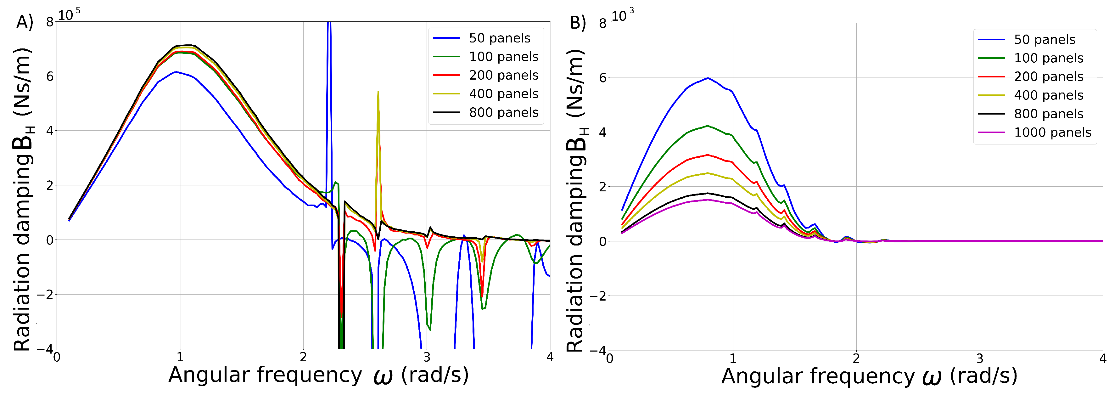
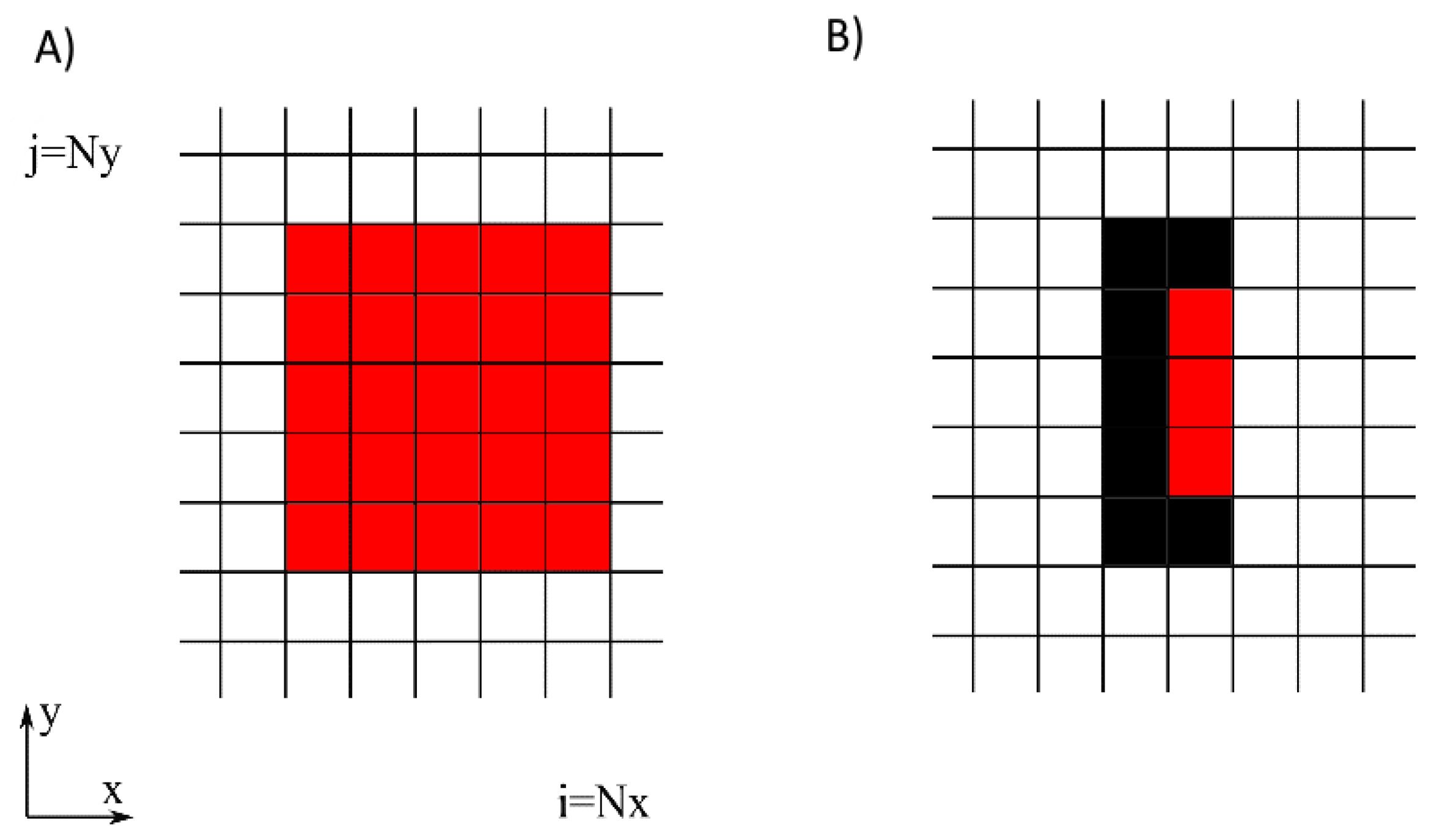
The accuracy between the two numerical approaches when modelling a single WEC is assessed by comparing the results from the MILDwave-NEMOH coupled model and the results from applying the sponge layer technique in MILDwave. A mesh convergence analysis was performed in NEMOH for the two WEC types. As seen in Figure 2A,B, convergent results for the hydrodynamic damping, , were obtained for 400 and 800 panels for the HPA WEC and OSWEC, respectively. Then, the total wave field around each single WEC type in NEMOH using a sub-optimal PTO, , in an area of 800 × 800 m was obtained. This total wave field was used as the representation of the “near-field” effects of the wave-structure interaction problem for tuning the MILDwave absorption coefficients for each set of wave conditions. The HPA WEC in MILDwave i represented by a group of grid cells forming an = 5 × = 5 grid cell configuration, as indicated in Figure 3A, while the OSWEC is represented by a group of grid cells forming an = 2 × = 5 grid cell configuration as indicated in Figure 3B. A grid cell size of dx = dy = 4.8 m was chosen for all simulations.
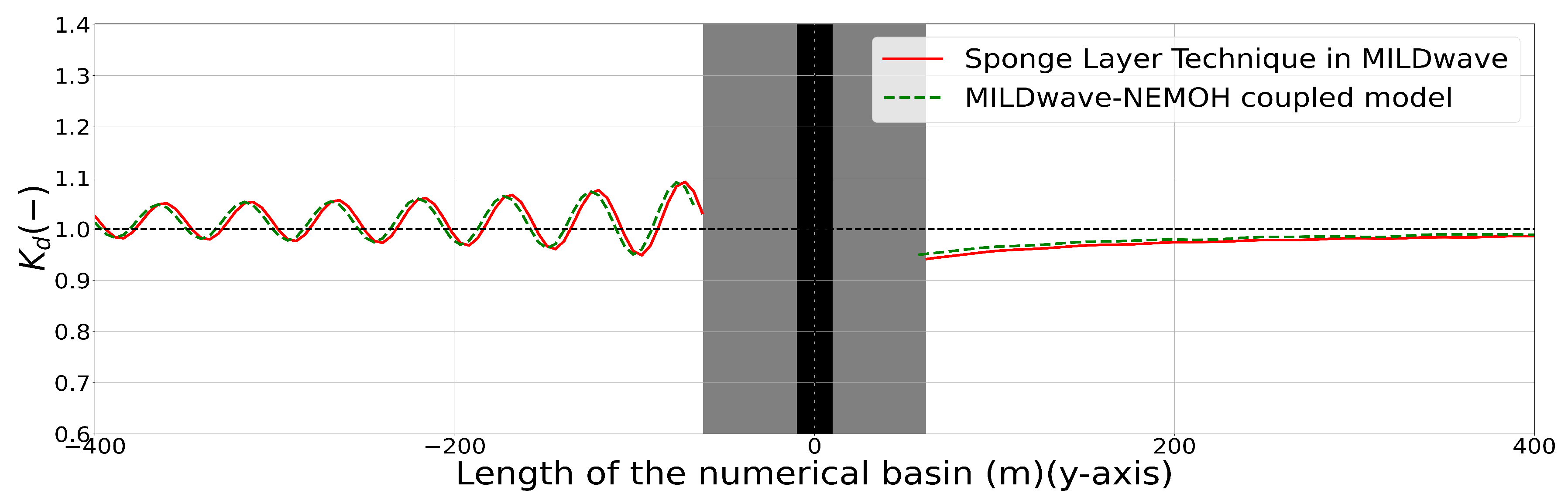
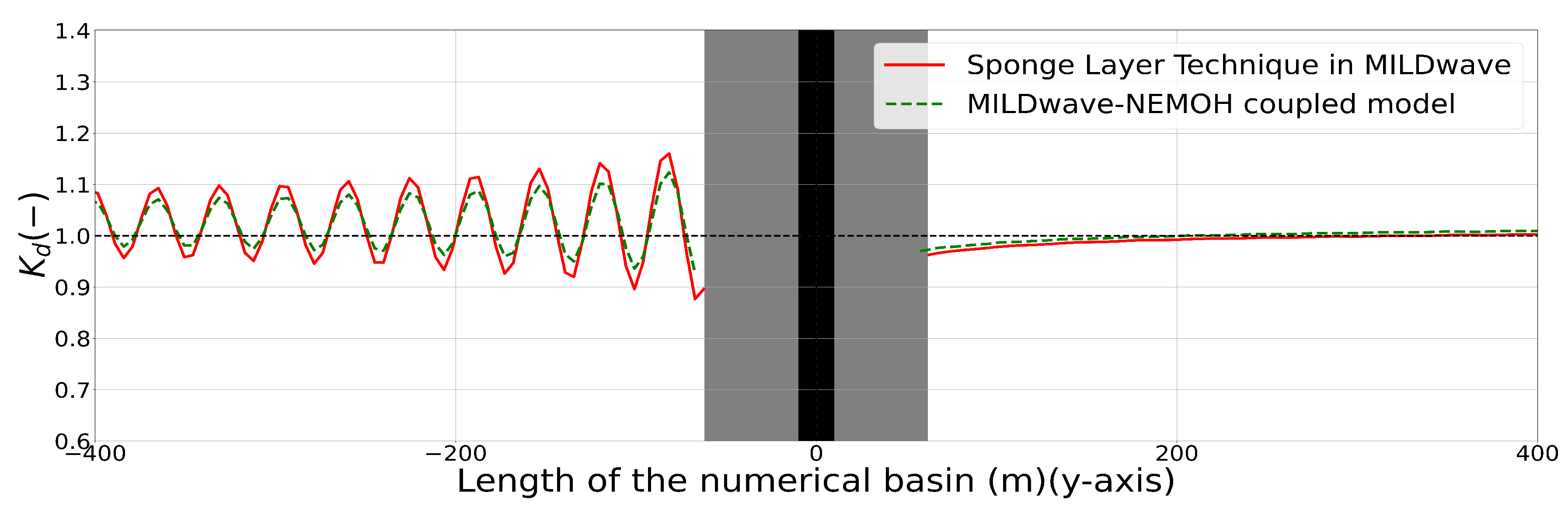
A sensitivity analysis for the wave absorption coefficients of the grid cells representing the WECs was performed in MILDwave until a convergent solution for the results between MILDwave and the MILDwave-NEMOH coupled model was obtained in the studied area. Figure 4 and Figure 5 show the results through the centre of the numerical domain at x = 0 m (a plan view of the x-y axis is included in Figure 6) for a single HPA WEC and a single OSWEC interacting with regular waves with m and s, respectively. It can be seen that the difference is quite high close to the WEC; however, this difference reduces drastically in the lee of the WEC after 100 m and especially after 400 m. Therefore, it is possible to obtain a good representation of the “far-field effects” at the lee of a single HPA WEC and OSWEC using the sponge layer technique. As indicated in Table 1, the % difference after 100 m for all test cases in MILDwave and the MILDwave-NEMOH coupled model never exceeds 3%. Furthermore, this difference becomes smaller when the ratio between the effective length of the WECs and the wave length decreases, as the interaction between the objects and the waves is reduced. Therefore, the parametrization in MILDwave obtained for a single WEC will be used in the following section to model a WEC farm using the sponge layer technique. The same wave absorption coefficient for each of the WECs of the farm will be employed.
3.1.2. WEC Farm
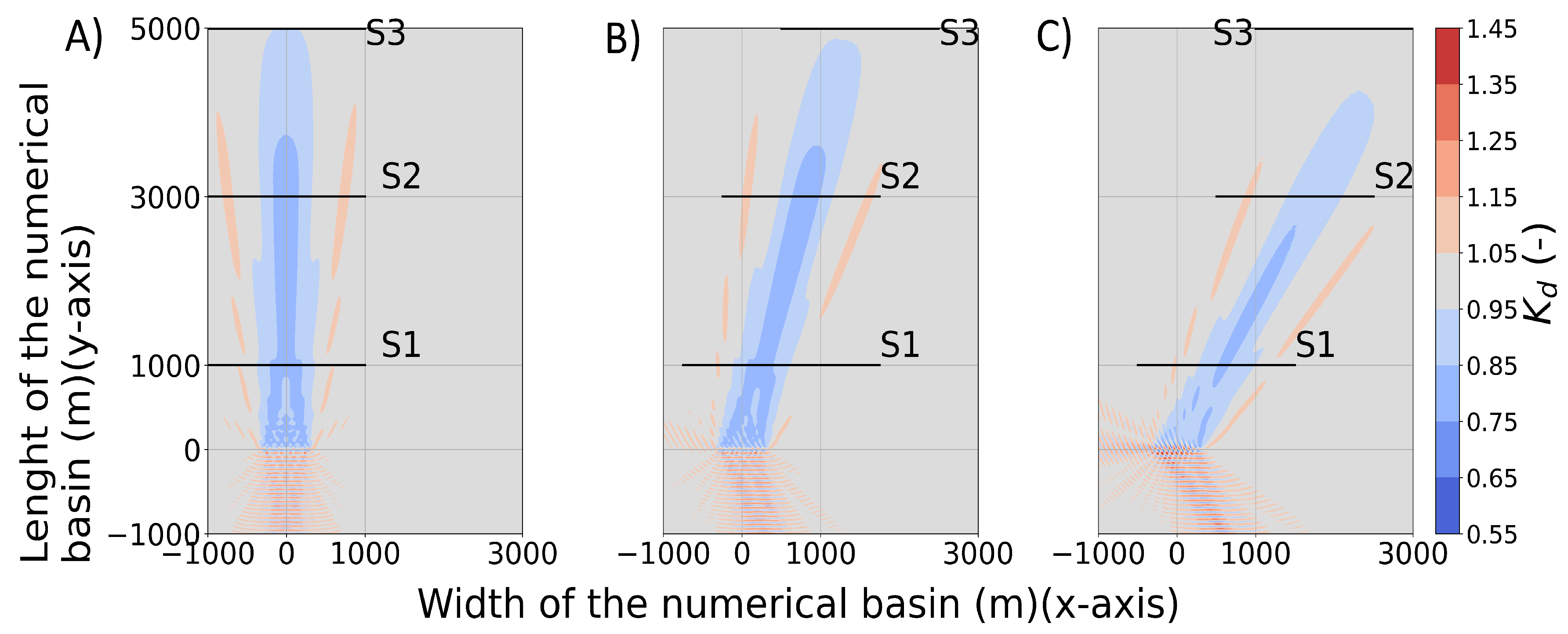
The “far-field” effects of two different WEC farms of 21 HPA WECs and OSWECs respectively are studied in this section using the MILDwave-NEMOH coupled model and the sponge layer technique in MILDwave. Figure 6A shows the for the MILDwave-NEMOH coupled model for a WEC farm of 21 HPA interacting with a regular wave with m, s and = 0°. It can be seen that the wave height is reduced in the direct lee of the WEC farm by up to 20% at a distance of 1000 m (location of S1). At 3000 m from the WEC farm (at S2), the wave field is still affected with a significant wave height reduction of 18%. Nevertheless, after 5000 m (at S3), this wave height reduction is limited to due to the effect of wave diffraction around the WECs and the damping of radiation. Results from the same wave, but with two different wave directions, = 15° and = 30°, are shown in Figure 6B,C, respectively. It can be observed that the wave height reduction in the lee of the HPA WEC farm is quantitatively similar for the three cases, with a variation of the “far field” effects’ alignment matching the incident wave direction.
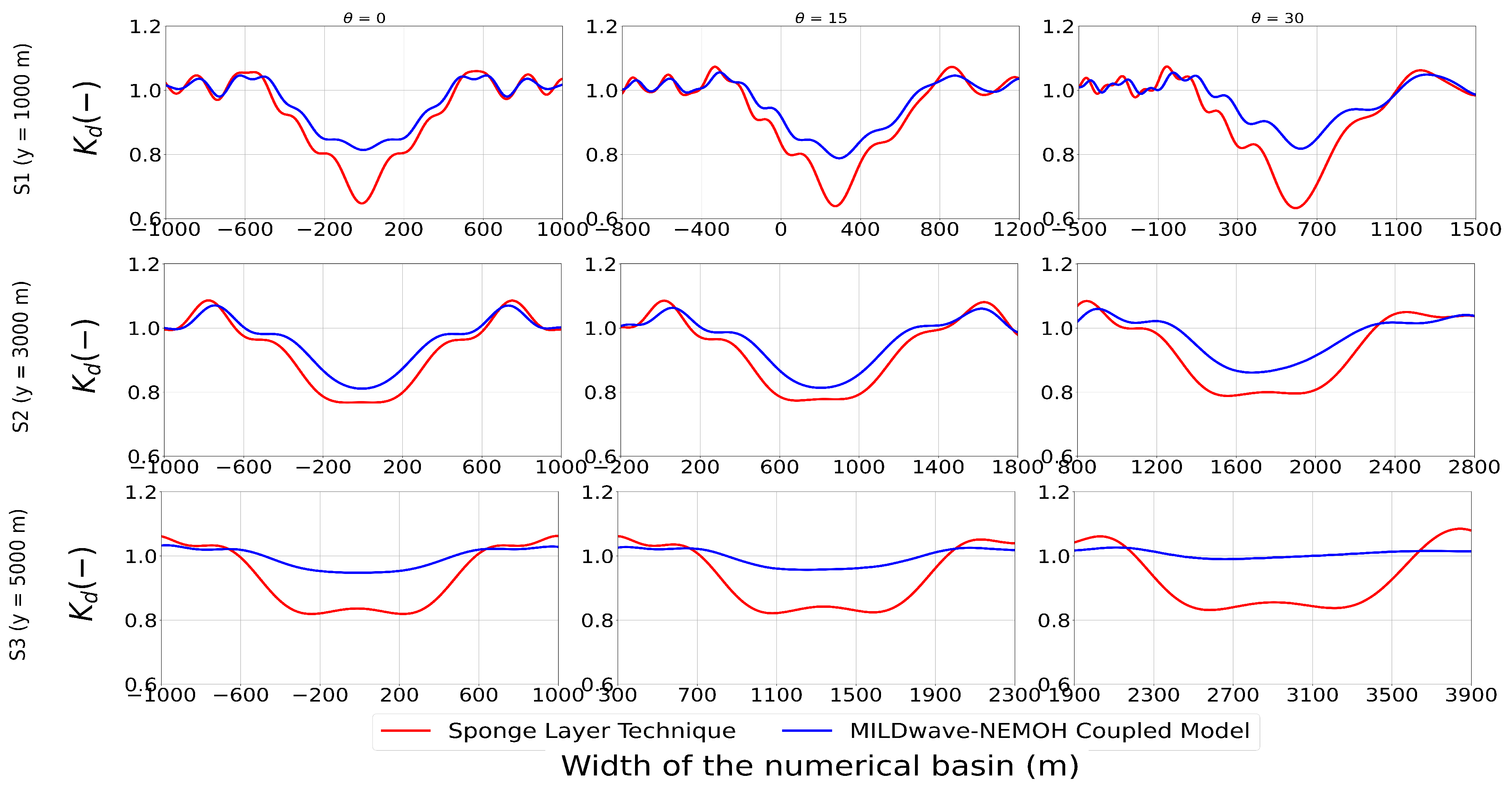
Figure 7 shows results at three transversal cross-sections (indicated in Figure 6) at y = 1000 m (S1), at y = 3000 m (S2) and at y = 5000 m (S3), for the MILDwave-NEMOH coupled model and the sponge layer technique, respectively, for a WEC farm of 21 HPA interacting with a regular wave with m and s. It can be noticed that both modelling approaches have the same behaviour in terms of wave height reduction in the direct lee of the WEC farm and with regard to the wave attenuation with the separating distance of the WECs in the WEC farm. Nevertheless, the order of the magnitude of this wave height reduction is higher when the sponge layer technique is applied. At a distance of 1000 m in the lee of the WEC farm, the wave height reduction reaches 30%. This wave height reduction goes down faster than in the MILDwave-NEMOH coupled model at a distance of 3000 m, reaching a 22% reduction of the wave height. However, at a distance of 5000 m, this reduction still remains at 17%.
The results of the eighteen test cases are summarized in Table 2. It can be observed that for all the test cases corresponding to the 21 HPA WEC farm, there is on average a difference in at a distance of y = 5000 m in the lee of the WEC farm; while for the 21 OSWEC farm, this average difference in is reduced to . This shows that the sponge layer technique is overestimating the “wake-effects” in the lee of the WEC farm. The sponge layer technique is based on absorbing energy from the incident waves over the entire water column, neglecting radiation effects. For the case of a single WEC, it is able to mimic the in the lee of the WEC as few absorbing cells are used to model a WEC. When increasing the number of WECs, radiation effects reduce exponentially with the distance to the WEC location and are almost not noticeable after 5000 m, as can be seen in the MILDwave-NEMOH coupled model. However, the effect of the absorbing cells in the MILDwave model is more persistent over distance when a high number of cells are used in a closely spaced manner to replicate a WEC farm.
3.2. PTO Modelling Techniques in the MILDwave-NEMOH Coupled Model
3.2.1. Power Production
As an intermediate step to study the “far-field” effects of the 21 HPA and 21 OSWEC farms, it is necessary to study the average power output of the two farms considered. The total power output is directly connected with the motions of the WEC’s floating bodies and therefore with the radiated and diffracted wave fields propagated in the lee of the WEC farm. The average power output for a single WEC, , of each type using a linear PTO, was obtained using Equation (5), while for the hydraulic PTO, Equations (8) and (9) were used. The results for the average power output using the three PTO systems and the test cases indicated in Section 2 for a single WEC, the 21 WEC farm and the q factor are included in Table 3 and Table 4 for the HPA and OSWEC, respectively. The q factor is defined as the ratio of the power of the N-WEC farm, , to the power produced by the sum of N WECs as if they were operating in isolation:
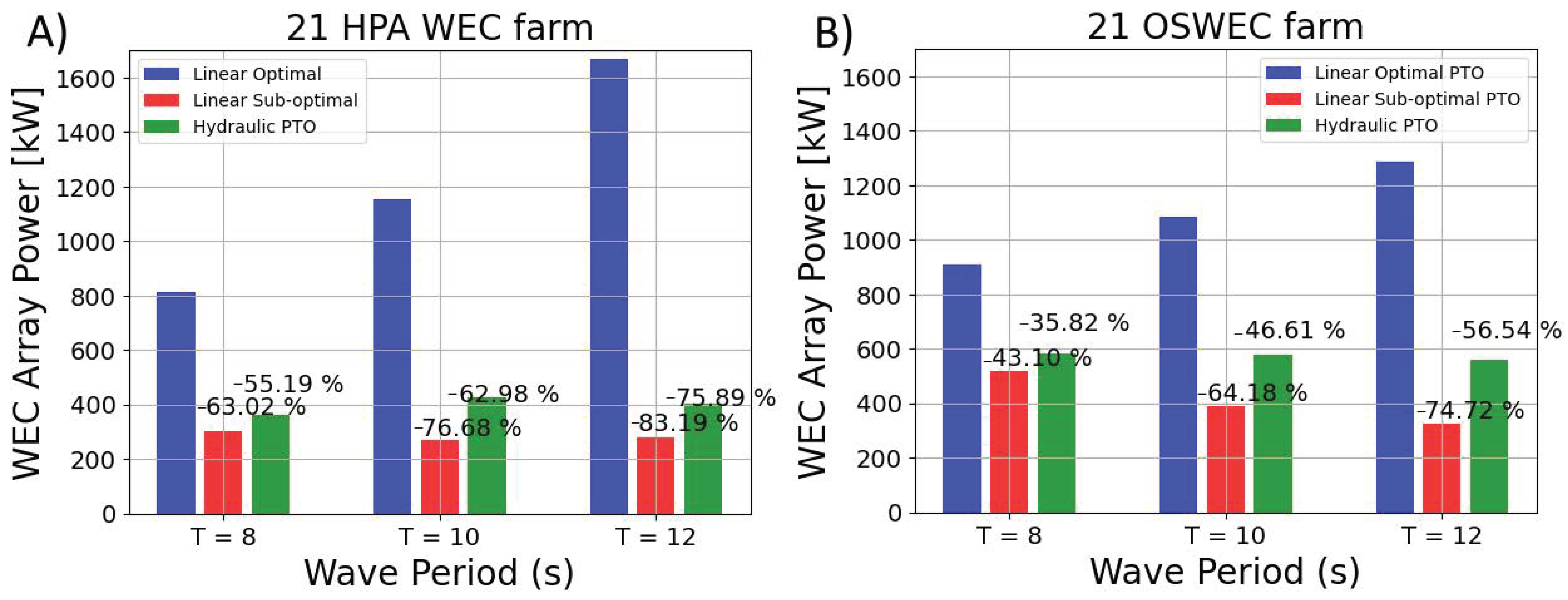
For a single WEC, it can be seen that there is a notable difference in the power output of the linear optimal PTO system compared to the sub-optimal and hydraulic PTOs, especially when the wave period is increased. In the optimal PTO system, the phase of the excitation force matches the velocity of the body, resulting in a much higher power output than the other two PTO systems. As can be seen in Figure 8, for an incident wave angle perpendicular to the WEC farm (), the linear optimal PTO shows on average more than a improvement in the power performance. Nonetheless, it has to be noted that for such a simplified linear optimal PTO system with no external elements damping the motion of the body, the methodology used may be making unrealistic assumptions about the motion of the body, resulting in an increased average power output, which can have a direct impact on the wave field simulations. Figure 8 also shows an average power output increase of for the hydraulic PTO with respect to the sub-optimal PTO. As indicated by [46], the hydraulic PTO system damps the motion of the WEC, matching the phase of the incoming waves, resulting in a higher power output than the sub-optimal linear WEC. Additionally, it can be observed that for most of the cases, the OSWEC is more efficient in absorbing the wave power than the HPA WEC, giving a higher power absorption for a single WEC.
For the WEC farm case, an increased power production is observed for the OSWEC farm except for the linear optimal PTO of the HPA WEC farms with wave periods s and s. The HPA and OSWEC farms produce less power with an increasing wave period. This is directly shown in the decreasing q values of the HPA WEC and OSWEC farms, which indicate that this specific configuration of the WEC farms is disadvantageous, even though the total power average for the OSWEC farm is increased with respect to the HPA WEC farm. Finally, it can be seen from the q factor that the incident wave angle, , has a direct impact on decreasing the performance of both WEC farms with reduced q values for all the PTO systems studied and consequently a reduced average power output. This reduction is more significant for the OSWECs, where the incident angle has a higher impact on reducing the motion of the body. Additionally, the OSWEC is placed in shallow water and occupies the entire water column, creating a shadowing effect due to wave diffraction and wave reflection in the WEC farm that are more significant than the shadowing effect created by the HPAs WEC farm.
3.2.2. “Far-Field” Effects
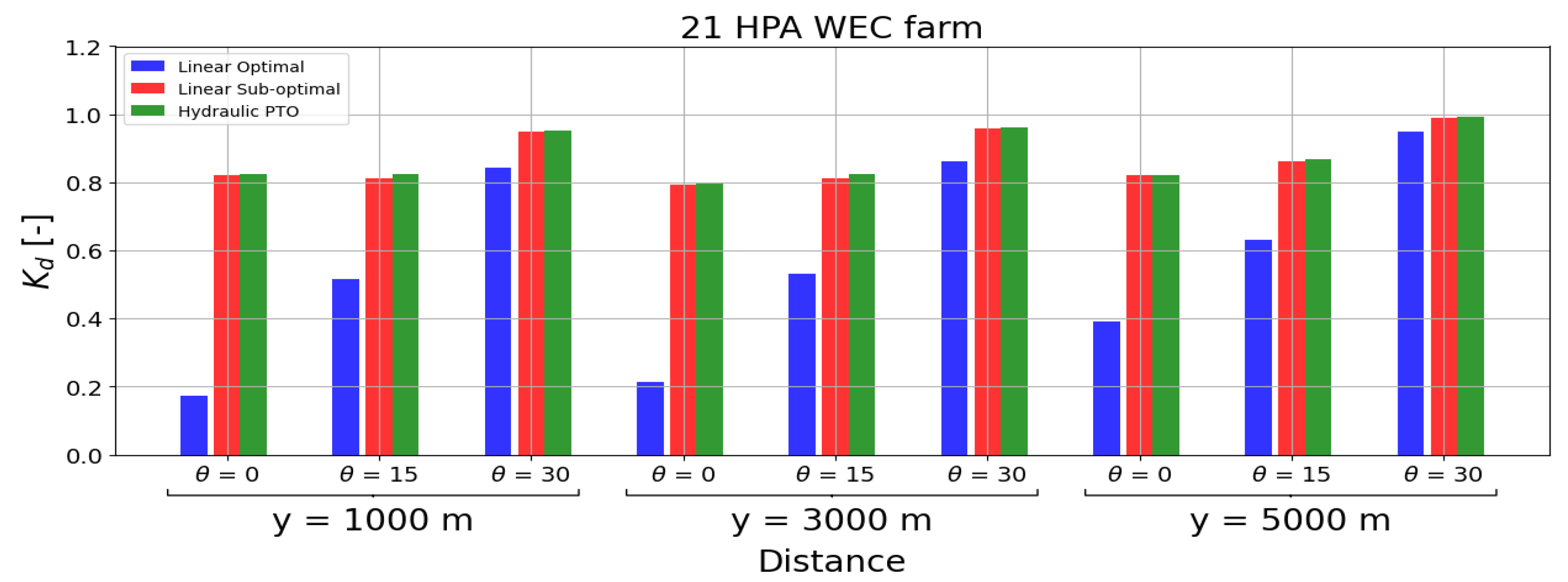
In this section, the “far-field” effects for a farm of 21 HPAs WECs and a farm of 21 OSWECs with different ways of simulating the PTO system are quantified using the disturbance coefficient, , and the average power production of the WEC farm discussed in Section 3.2.1. Using the MILDwave-NEMOH coupled model for the test cases indicated in Section 2, the total wave field around the two different WEC farms is obtained. The minimum values (indicating the maximum wave height reduction) at a distance of y = 1000 m (S1), y = 3000 m (S2) and y = 5000 m (S3) in the lee of the WEC farm is quantified and summarized in Table 5 and Table 6, for the HPA WEC farm and the OSWEC farm, respectively.
Looking at the two WEC farms studied, it can be determined that the “far-field” effects are much stronger for the 21 OSWEC farm case than for the 21 HPA WEC farm case. In comparing Table 5 and Table 6, it can be seen that the values are much lower for the OSWEC farm, especially at a distance of y = 1000 m (S1) in the lee of the WEC farm. The difference in the magnitude so close to the WEC farm is due to the difference in the behaviour of the two WEC types and their impact on the “near-field”. As previously mentioned in Section 3.2.1, the OSWEC is operating in shallow water and occupies the entire water column, presenting a bigger obstacle to the incoming waves, resulting in a higher diffraction than the HPAs. Additionally, the OSWEC generates a significant radiated field. The influence of both phenomena on the “near-field” was studied by [46], indicating that for the OSWEC, the areas of increased and reduced wave height close to the OSWECs can be up to larger than those of the HPA WECs, and at a distance of y = 1000 m (S1) from the WEC farms, this effect is still persistent. When moving further down wave in the lee of the WEC farm at distances of y = 3000 m (S2) and y = 5000 m (S3), a difference in the values also exists, but they are significantly reduced in most of the test cases. The values for both WEC types are over in magnitude, indicating less than a reduction in wave height. When the distance to the WEC farm starts to be significant, the wave radiation effects due to the WEC are significantly diminished. This factor in combination with the constructive effect of wave diffraction contributes to the observation that in the “far-field”, both types of WEC farms have a similar impact on the wave height reduction.
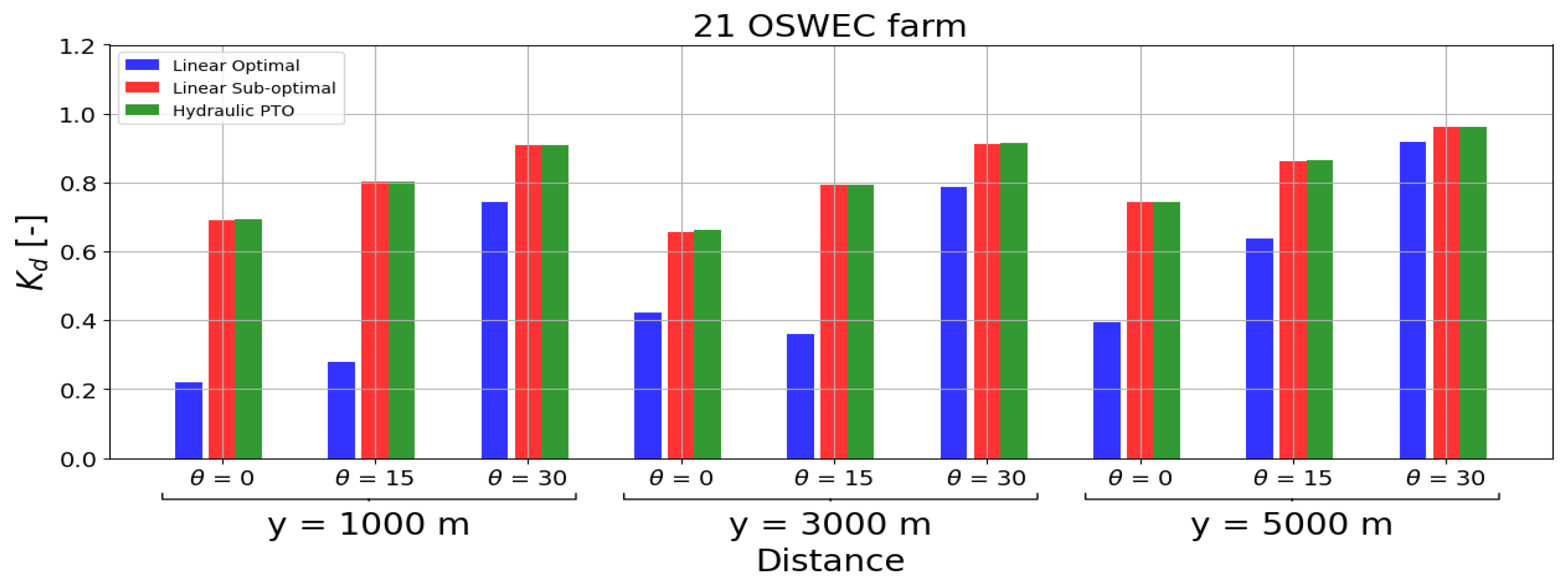
To closely examine the effect of the PTO system in the “far-field”, two bar charts are presented (Figure 9 and Figure 10) showing the values for the three modelled PTO systems, for m, s, at three different locations in the lee of the WEC farms (y = 1000 m, y = 3000 m and y = 5000 m). It can be observed that the optimal linear PTO gives consistently a much lower for both the OSWEC farm and HPA WEC farm than that given by the sub-optimal and hydraulic PTOs. The values for all PTO systems are increased when the incident wave angle, increases from 0° to 30°. However, when increasing the wave period, T, a different trend can be observed in Table 5 and Table 6. For the sub-optimal and hydraulic PTO system, the values increase by increasing the wave period, while for the optimal PTO system, there is a reduction. This anomaly in the results for the optimal PTO representation with s and s can be explained in conjunction with the power output obtained in Section 3.2.1. Due to the approach used to obtain the motions of the WECs for the optimal PTO system, the average power output obtained in Section 3.2.1 indicates an overestimation of the WEC motions for both the HPA WEC and the OSWEC, especially for the higher periods. Consequently, this has an impact on the wave field transferred to the MILDwave-NEMOH coupled model with values at y = 1000 m in the lee of the WEC farms lower than 0.1 in magnitude. Despite a low magnitude close to the WEC farm, the at a distance of y = 5000 m (S3) has an overall increase of 0.4 in magnitude for the optimal PTO system. This result indicates that in the “far-field”, the damping of the wave radiation effect is playing a major role.
3.2.3. Effect of the PTO System in the “Far-Field”
In this section, the interplay between the three PTO systems, the average power output and the “far-field” effects of the WEC farms is studied. Primarily, the linear optimal PTO system impact at a distance of y = 1000 m (S1) in the lee of the WEC farm is much higher than for the linear sub-optimal and hydraulic PTOs. This is aligned with a higher average power output, as seen in Figure 8, especially for the cases of s and s. Contrary to the optimal PTO system, the sub-optimal and hydraulic PTO systems have very similar values at y = 1000 m (S1) for all the test cases, with a very different behaviour in the power output. For both PTO systems, it can be observed that is increased with an increase of both the wave period and the incident wave angle. This matches a reduction of the average power output of the WEC farms, as seen in Table 3 and Table 4. Yet, the values for both the sub-optimal and hydraulic PTO are very similar. As shown in Figure 8, the hydraulic PTO system consistently gives on average a greater power output than the sub-optimal PTO system for both the HPA and OSWEC farms. At larger distances from the WEC farms (y = 3000 (S2) and y = 5000 m (S3)), the values are almost close to one, indicating that for these two PTO systems, the WEC farm performance due to a change in the PTO has no impact on the “far-field”. However, for the optimal PTO system, there is a meaningful impact on the “far-field” with a magnitude around 0.4. Nevertheless, this magnitude is increasing rapidly with the distance to the WEC farm, indicating that the larger the distance to the WEC farm, the lower the WEC farm impact on the wave field is.
It is clear that there is a contrasting behaviour between the three PTO systems in terms of wave energy production that is not evenly represented in the “far-field”. Such a different behaviour is due to the hydrodynamics of the two WECs under the different PTO systems. In the case of the optimal and sub-optimal PTO system, the PTO external damping is included in the equation of motion. The optimal PTO system drastically increases the body motion, changing the phase of the WEC and forcing it to resonate. With regard to the hydraulic PTO as indicated by [46], the primary driver in the increase of the PTO average power output is the increase in the PTO system force, which also has an impact on the WEC motion. It has to be stressed that in the present study, a linear hydrodynamic model is used for simulating the WEC farms under the action of regular waves. It has been shown in previous research from the authors that this assumption tends to overestimate the “far-field” effects, motions and power output of the WEC farm. The motions of the WECs under an irregular waves scenario will be reduced considerably, as well as the effectiveness of the PTO system. Therefore, the differences in the “far-field” effects for different PTO systems will be even smaller. This indicates that, for calculating the average power output of a WEC farm, it is important to correctly model the PTO system. Due to the small differences in WEC motions and the rapid decrease of the wave radiation effect with the distance to the WEC farm, a less complex PTO approach can be considered when calculating the “far-field” effects.
4. Conclusions
In this research, the difference in accuracy when calculating the “far-field” effects of different WEC farms under regular waves for a parameterized model and a numerically coupled model was studied. The MILDwave sponge layer technique and the MILDwave-NEMOH coupled model were compared in terms of wave height reduction in the lee of the WEC array. Based on this comparison, the effect of the PTO system in the “far-field” was demonstrated for three types of PTO systems, namely a linear optimal, a linear sub-optimal and a hydraulic PTO; calculating both the average power production of the farm and the in the “far-field”.
Firstly, when comparing the sponge layer technique and the MILDwave-NEMOH coupled model, it was shown that the sponge layer technique gives reduced values of for all test cases compared to those resulting from the coupled model. At a large distance to the WEC farm (y = 5000 m (S3)), the difference in remains for the HPA farm and is reduced to for the OSWEC farm. The sponge layer technique performs better when mimicking the behaviour of an OSWEC, as OSWECs occupy the whole water column; however, it considerably overestimates the wave height reduction in the lee of the WEC farm. Therefore, the use of a coupled model where the body hydrodynamics are simulated is preferred. Secondly, it was demonstrated that when using a coupled model, it is necessary to carefully model the motions of the WEC to not overestimate the “far-field” effects. It is observed that for an optimal linear PTO system, where unrealistic WEC motions are present, is highly reduced at a large distance to the WEC farm (y = 5000 m (S3)). However, for the sub-optimal and hydraulic PTO, where the motions of the WEC are still within the assumptions of small amplitude WEC motions of the linear numerical models used, at a distance of y = 5000 m (S3) is close to one and remains in the same order of magnitude for both PTO systems in all the test cases. Thirdly, it is shown that an increase in the average power output moving from a linear sub-optimal PTO to a hydraulic PTO does not have an impact on the “far-field”. Consequently, if optimizing the power output is not the main target of an WEC farm study, modelling the PTO effect by using a linear sub-optimal PTO system is sufficient to study WEC farm “far-field” effects.
It can be concluded that in order to avoid overestimating the “far-field” effects of WEC farms, it is more accurate to use a coupled model numerical approach. This is because the difference in the assessed impact on the surrounding wave field can be substantial, especially for a WEC farm with a large number of WECs. Nonetheless, when using coupled models, it is necessary to carefully model the hydrodynamics of the WEC. As demonstrated in this research, an incorrect modelling of the PTO system can, e.g., result in overestimating the WECs’ motion within the farm, which can introduce substantial inaccuracies into the wave field calculation.
Author Contributions
G.V.F. and N.Q. set up the numerical experiments. V.S. and P.T. provided the foundation of the coupling methodology. G.V.F. implemented the MILDwave-NEMOH coupled model. V.S. and P.T. proofread the text and helped in structuring the publication. All authors read and agreed to the published version of the manuscript.
Funding
Vasiliki Stratigaki is a post-doctoral researcher (fellowship 1267321N) of the FWO, Belgium. Nicolas Quartier is a Ph.D. fellow (fellowship 1SC5419N) of the FWO, Belgium.
Institutional Review Board Statement
Not applicable.
Informed Consent Statement
Not applicable.
Data Availability Statement
Not applicable.
Acknowledgments
Vasiliki Stratigaki is a post-doctoral researcher (fellowship 1267321N) of the FWO (Fonds Wetenschappelijk Onderzoek—Research Foundation Flanders), Belgium.
Conflicts of Interest
The authors declare no conflict of interest.
Abbreviations
The following abbreviations are used in this manuscript:
| TRL | technology readiness level |
| WEC | wave energy converter |
| SPH | smoothed particle hydrodynamics |
| BEM | boundary element method |
| CFD | computer fluid dynamics |
| DoF | degree of freedom |
| PTO | power take-off |
| RAO | response amplitude operator |
| HPA | heaving point absorber |
| OSWEC | oscillating wave surge wave energy converter |
References
- Weber, J.; Costello, R.; Ringwood, J. WEC Technology Performance Levels (TPLs)—Metric for Successful Development of Economic WEC Technology. In Proceedings of the 10th European Wave and Tidal Energy Conference, Aalborg, Denmark, 2–5 September 2013. [Google Scholar]
- Stratigaki, V. WECANet: The First Open Pan-European Network for Marine Renewable Energy with a Focus on Wave Energy-COST Action CA17105. Water 2019, 11, 1249. [Google Scholar] [CrossRef] [Green Version]
- Millar, D.L.; Smith, H.C.M.; Reeve, D.E. Modelling analysis of the sensitivity of shoreline change to a wave farm. Ocean. Eng. 2007, 34, 884–901. [Google Scholar] [CrossRef]
- Delft University of Technology. SWAN (Simulating WAves Nearshore); A Third Generation Wave Model Copyright©1993–2020. 2020. Available online: http://swanmodel.sourceforge.net/features/features.htm/ (accessed on 11 November 2020).
- Smith, H.C.; Pearce, C.; Millar, D.L. Further analysis of change in nearshore wave climate due to an offshore wave farm: An enhanced case study for the Wave Hub site. Renew. Energy 2012, 40, 51–64. [Google Scholar] [CrossRef]
- Rusu, E.; Onea, F. Study on the influence of the distance to shore for a wave energy farm operating in the central part of the Portuguese nearshore. Energy Convers. Manag. 2016, 114, 209–223. [Google Scholar] [CrossRef]
- Onea, F.; Rusu, E. The Expected Shoreline Effect of a Marine Energy Farm Operating Close to Sardinia Island. Water 2019, 11, 2303. [Google Scholar] [CrossRef] [Green Version]
- Raileanu, A.; Onea, F.; Rusu, E. An Overview of the Expected Shoreline Impact of the Marine Energy Farms Operating in Different Coastal Environments. J. Mar. Sci. Eng. 2020, 8, 228. [Google Scholar] [CrossRef] [Green Version]
- Iglesias, G.; Carballo, R.; Castro, A. Development of the WaveCat wave energy converter. In Proceedings of the 31st International Conference of Coastal Engineering, Hamburg, Germany, 31 August–5 September 2008. [Google Scholar]
- Carballo, R.; Iglesias, G. Wave farm impact based on realistic wave-WEC interaction. Energy 2013, 51, 216–229. [Google Scholar] [CrossRef]
- Fernandez, H.; Iglesias, G.; Carballo, R.; Castro, A.; Fraguela, J.; Taveira-Pinto, F.; Sanchez, M. The new wave energy converter WaveCat: Concept and laboratory tests. Mar. Struct. 2012, 29, 58–70. [Google Scholar] [CrossRef]
- Iglesias, G.; Carballo, R. Wave farm impact: The role of farm-to-coast distance. Renew. Energy 2014, 69, 375–385. [Google Scholar] [CrossRef]
- Abanades, J.; Greaves, D.; Iglesias, G. Coastal defence using wave farms: The role of farm-to-coast distance. Renew. Energy 2015, 75, 572–582. [Google Scholar] [CrossRef] [Green Version]
- XBeach Open Source Community. XBeach. 2019. Available online: https://oss.deltares.nl/web/xbeach/ (accessed on 6 June 2019).
- Chang, G.; Ruehl, K.; Jones, C.; Roberts, J.; Chartrand, C. Numerical modelling of the effects of wave energy converter characteristics on nearshore wave conditions. Renew. Energy 2016, 89, 636–648. [Google Scholar] [CrossRef] [Green Version]
- Beels, C.; Troch, P.; De Backer, G.; Vantorre, M.; De Rouck, J. Numerical implementation and sensitivity analysis of a wave energy converter in a time-dependent mild-slope equation model. Coast. Eng. 2010, 57, 471–492. [Google Scholar] [CrossRef]
- Tuba Özkan-Haller, H.; Haller, M.C.; Cameron McNatt, J.; Porter, A.; Lenee-Bluhm, P. Analyses of Wave Scattering and Absorption Produced by WEC Arrays: Physical/Numerical Experiments and Model Assessment. In Marine Renewable Energy: Resource Characterization and Physical Effects; Springer International Publishing: Cham, Switzerland, 2017; pp. 71–97. [Google Scholar] [CrossRef]
- Stokes, C.; Conley, D. Modelling Offshore Wave farms for Coastal Process Impact Assessment: Waves, Beach Morphology, and Water Users. Energies 2018, 11, 2517. [Google Scholar] [CrossRef] [Green Version]
- Davidson, J.; Costello, R. Efficient Nonlinear Hydrodynamic Models for Wave Energy Converter Design: A Scoping Study. J. Mar. Sci. Eng. 2020, 8, 35. [Google Scholar] [CrossRef] [Green Version]
- Giorgi, G.; Ringwood, J.V. Articulating Parametric Nonlinearities in Computationally Efficient Hydrodynamic Models. IFAC-PapersOnLine 2018, 51, 56–61. [Google Scholar] [CrossRef]
- Magana, M.E.; Brown, D.R.; Gaebelle, D.T.; Henriques, J.C.; Brekken, T.K. Sliding Mode Control of an Array of Three Oscillating Water Column Wave Energy Converters to Optimize Electrical Power. In Proceedings of the 13th European Wave and Tidal Energy Conference, Napoli, Italy, 1–6 September 2019. [Google Scholar]
- Gaebele, D.; Magaña, M.; Brekken, T.; Sawodny, O. State space model of an array of oscillating water column wave energy converters with inter-body hydrodynamic coupling. Ocean. Eng. 2020, 195, 106668. [Google Scholar] [CrossRef]
- Crespo, A.; Altomare, C.; Domínguez, J.; González-Cao, J.; Gómez-Gesteira, M. Towards simulating floating offshore oscillating water column converters with Smoothed Particle Hydrodynamics. Coast. Eng. 2017, 126, 11–26. [Google Scholar] [CrossRef]
- Verbrugghe, T.; Domínguez, J.M.; Crespo, A.J.; Altomare, C.; Stratigaki, V.; Troch, P.; Kortenhaus, A. Coupling methodology for smoothed particle hydrodynamics modelling of non-linear wave-structure interactions. Coast. Eng. 2018, 138, 184–198. [Google Scholar] [CrossRef]
- Domínguez, J.M.; Crespo, A.J.; Hall, M.; Altomare, C.; Wu, M.; Stratigaki, V.; Troch, P.; Cappietti, L.; Gómez-Gesteira, M. SPH simulation of floating structures with moorings. Coast. Eng. 2019, 153, 103560. [Google Scholar] [CrossRef]
- Ransley, E.; Yan, S.; Brown, S.; Musiedlak, P.H.; Windt, C.; Schmitt, P.; Davidson, J.; Ringwood, J.; Wang, J.; Wang, J. A blind comparative study of focused wave interactions with floating structures (CCP-WSI Blind Test Series 3). Int. J. Offshore Polar Eng. 2019, 29. [Google Scholar] [CrossRef] [Green Version]
- Windt, C.; Davidson, J.; Schmitt, P.; Ringwood, J. Contribution to the CCP-WSI Blind Test Series 3: Analysis of scaling effects of moored point-absorber wave energy converters in a CFD-based numerical wave tank. In Proceedings of the 29th International Ocean and Polar Engineering Conference, Honolulu, HI, USA, 16–21 June 2019. [Google Scholar]
- Liu, Z.; Wang, Y.; Hua, X. Numerical studies and proposal of design equations on cylindrical oscillating wave surge converters under regular waves using SPH. Energy Convers. Manag. 2020, 203, 112242. [Google Scholar] [CrossRef]
- Ransley, E.; Greaves, D.; Raby, A.; Simmonds, D.; Hann, M. Survivability of wave energy converters using CFD. Renew. Energy 2017, 109, 235–247. [Google Scholar] [CrossRef] [Green Version]
- Devolder, B.; Stratigaki, V.; Troch, P.; Rauwoens, P. CFD simulations of floating point absorber wave energy converter arrays subjected to regular waves. Energies 2018, 11, 641. [Google Scholar] [CrossRef] [Green Version]
- Abbasnia, A.; Soares, C.G. Fully nonlinear simulation of wave interaction with a cylindrical wave energy converter in a numerical wave tank. Ocean. Eng. 2018, 152, 210–222. [Google Scholar] [CrossRef]
- Kim, S.; Koo, W. Numerical simulation of a latching controlled heaving-buoy-type point absorber by using a 3D numerical wave tank. In Proceedings of the 13th European Wave and Tidal Energy Conference (EWTEC 2019), Napoli, Italiy, 1–6 September 2019. [Google Scholar]
- Giorgi, G.; Gomes, R.P.F.; Bracco, G.; Mattiazzo, G. The Effect of Mooring Line Parameters in Inducing Parametric Resonance on the Spar-Buoy Oscillating Water Column Wave Energy Converter. J. Mar. Sci. Eng. 2020, 8, 29. [Google Scholar] [CrossRef] [Green Version]
- Charrayre, F.; Peyrard, C.; Benoit, M.; Babarit, A. A Coupled Methodology for Wave-Body Interactions at the Scale of a Farm of Wave Energy Converters Including Irregular Bathymetry. In Proceedings of the ASME 2014 33rd International Conference on Ocean, Offshore and Arctic Engineering, San Francisco, CA, USA, 8–13 June 2014. [Google Scholar]
- Balitsky, P.; Verao Fernandez, G.; Stratigaki, V.; Troch, P. Coupling methodology for modelling the near-field and far-field effects of a Wave Energy Converter. In Proceedings of the ASME 36th International Conference on Ocean, Offshore and Arctic Engineering, Trondheim, Norway, 25–30 June 2017. [Google Scholar]
- Tomey-Bozo, N.; Babarit, J.M.A.; Troch, P.; Lewis, T.; Thomas, G. Wake Effect Assesment of a flap-type wave energy converter farm using a coupling methodology. In Proceedings of the ASME 36th International Conference on Ocean, Offshore and Arctic Engineering, Trondheim, Norway, 25–30 June 2017. [Google Scholar]
- Fernandez, G. A Numerical Study of the Far Field Effects of Wave Energy Converters in Short and Long-Crested Waves Utilizing a Coupled Model Suite. Ph.D. Thesis, Ghent University, Ghent, Belgium, 2019. [Google Scholar]
- Verbrugghe, T.; Stratigaki, V.; Troch, P.; Rabussier, R.; Kortenhaus, A. A comparison study of a generic coupling methodology for modelling wake effects of wave energy converter arrays. Energies 2017, 10, 1697. [Google Scholar] [CrossRef] [Green Version]
- Kemper, J.; Windt, C.; Graf, K.; Ringwood, J.V. Development towards a nested hydrodynamic model for the numerical analysis of ocean wave energy systems. In Proceedings of the 13th European Wave and Tidal Energy Conference, Naples, Italy, 1–6 September 2019. [Google Scholar]
- Rijnsdorp, D.P.; Hansen, J.E.; Lowe, R.J. Simulating the wave-induced response of a submerged wave-energy converter using a non-hydrostatic wave-flow model. Coast. Eng. 2018, 140, 189–204. [Google Scholar] [CrossRef]
- Rijnsdorp, D.P.; Hansen, J.E.; Lowe, R.J. Understanding coastal impacts by nearshore wave farms using a phase-resolving wave model. Renew. Energy 2020, 150, 637–648. [Google Scholar] [CrossRef]
- Tomey-Bozo, N.; Babarit, A.; Murphy, J.; Stratigaki, V.; Troch, P.; Lewis, T.; Thomas, G. Wake effect assessment of a flap type wave energy converter farm under realistic environmental conditions by using a numerical coupling methodology. Coast. Eng. 2018. [Google Scholar] [CrossRef] [Green Version]
- Fernandez, G.; Balitsky, P.; Stratigaki, V.; Troch, P. Coupling Methodology for Studying the Far Field Effects of Wave Energy Converter Arrays over a Varying Bathymetry. Energies 2018, 11, 2899. [Google Scholar] [CrossRef] [Green Version]
- Stratigaki, V.; Troch, P.; Forehand, D. A fundamental coupling methodology for modelling near-field and far-field wave effects of floating structures and wave energy devices. Renew. Energy 2019, in press. [Google Scholar] [CrossRef]
- Balitsky, P.; Verao Fernandez, G.; Stratigaki, V.; Troch, P. Assessment of the Power Output of a Two-Array Clustered WEC Farm Using a BEM Solver Coupling and a Wave-Propagation Model. Energies 2018, 11, 2907. [Google Scholar] [CrossRef] [Green Version]
- Balitsky, P.; Quartier, N.; Stratigaki, V.; Verao Fernandez, G.; Vasarmidis, P.; Troch, P. Analysing the near-field effects and the power production of near-shore WEC array using a new wave-to-wire model. Water 2019, 11. [Google Scholar] [CrossRef] [Green Version]
- Verao Fernandez, G.; Stratigaki, V.; Troch, P. Irregular Wave Validation of a Coupling Methodology for Numerical Modelling of Near and Far Field Effects of Wave Energy Converter Arrays. Energies 2019, 12, 538. [Google Scholar] [CrossRef] [Green Version]
- Bingham, H. A hybrid Boussinesq-panel method for predicting the motion of a moored ship. Coast. Eng. 2000, 40, 21–38. [Google Scholar] [CrossRef]
- Agamloh, E.B.; Wallace, A.K.; von Jouanne, A. Application of fluid-structure interaction simulation of an ocean wave energy extraction device. Renew. Energy 2008, 33, 748–757. [Google Scholar] [CrossRef]
- McCallum, P.D. Numerical Methods for Modelling the Viscous Effects on the Interactions between Multiple Wave Energy Converters. Ph.D. Thesis, The University of Edinburgh, Edinburgh, UK, 2017. [Google Scholar]
- Babarit, A.; Delhommeau, G. Theoretical and numerical aspects of the open source BEM solver {NEMOH}. In Proceedings of the 11th European Wave and Tidal Energy Conference, Nantes, France, 6–11 September 2015. [Google Scholar]
- Penalba, M.; Kelly, T.; Ringwood, J. Using NEMOH for Modelling Wave Energy Converters: A Comparative Study with WAMIT. In Proceedings of the 12th European Wave and Tidal Energy Conference, Cork, Ireland, 27 August–1 September 2017. [Google Scholar]
- Troch, P. MILDwave—A Numerical Model for Propagation and Transformation of Linear Water Waves; Technical Report; Internal Report; Department of Civil Engineering, Ghent University: Ghent, Belgium, 1998. [Google Scholar]
- Troch, P.; Stratigaki, V. Phase-Resolving Wave Propagation Array Models. In Numerical Modelling of Wave Energy Converters; Folley, M., Ed.; Elsevier: Amsterdam, The Netherlands, 2016; Chapter 10; pp. 191–216. [Google Scholar] [CrossRef]
- Radder, A.C.; Dingemans, M.W. Canonical equations for almost periodic, weakly nonlinear gravity waves. Wave Motion 1985, 7, 473–485. [Google Scholar] [CrossRef]
- Vasarmidis, P.; Stratigaki, V.; Troch, P. Accurate and Fast Generation of Irregular Short Crested Waves by Using Periodic Boundaries in a Mild-Slope Wave Model. Energies 2019, 12, 785. [Google Scholar] [CrossRef] [Green Version]
- Stratigaki, V. Experimental Study and Numerical Modelling of Intra-Array Interactions and Extra-Array Effects of Wave Energy Converter Arrays. Ph.D. Thesis, Ghent University, Ghent, Belgium, 2014. [Google Scholar]
- European Marine Energy Centre (EMEC) Ltd. Wave Developers Database. Available online: http://www.emec.org.uk/marine-energy/wave-developers/ (accessed on 13 November 2018).
- Alves, M. Frequency-Domain Models. In Numerical Modelling of Wave Energy Converters; Folley, M., Ed.; Elsevier: Amsterdam, The Netherlands, 2016; Chapter 2; pp. 11–30. [Google Scholar] [CrossRef]
- Cargo, C. Design and Control of Hydraulic Power Take-Offs for Wave Energy Converters. Ph.D. Thesis, University of Bath, Bath, UK, 2013. [Google Scholar]
Figure 1.
(A) Low-order mesh for the HPA WEC; and (B) low-order mesh for the OSWEC.

Figure 2.
Mesh convergence study for (A) the HPA WEC and (B) the OSWEC for different panel discretizations.
Figure 2.
Mesh convergence study for (A) the HPA WEC and (B) the OSWEC for different panel discretizations.

Figure 3.
Detail from the sponge layer technique employed in MILDwave to mimic the behaviour of the WEC. In Subplot (A), the HPA WEC is represented by an = 5 × = 5 cell grid configuration. In Subplot (B), the OSWEC is represented by an = 2 × = 5 grid cell configuration. Black cells indicate fully reflective cells, while the red cells are assigned a specific wave absorption coefficient.

Figure 4.
Kd disturbance coefficient results for the MILDwave-NEMOH coupled model and the MILDwave sponge layer technique along one longitudinal cross-section at the centre of the domain for a single HPA WEC interacting with regular waves of H = 2 m and T = 8 s. The coupling region is filled in grey colour and includes the WEC’s cross-section indicated by a black vertical area. Incident waves are generated from the left to the right.

Figure 5.
Kd disturbance coefficient results for the MILDwave-NEMOH coupled model and the MILDwave sponge layer technique along one longitudinal cross-section at the centre of the domain for a single OSWEC interacting with regular waves of H = 2 m and T = 8 s. The coupling region is filled in grey colour and includes the WEC’s cross-section indicated by a black vertical area. Incident waves are generated from the left to the right.

Figure 6.
disturbance coefficient results for a 21 HPA WEC farm interacting with regular waves of m, s and (A) = 0°, (B) 15° and (C) 30° in the MILDwave-NEMOH coupled model. S1, S2 and S3 indicate the locations of the cross-sections. Contour levels are set at an interval of 0.05 for the value. The water depth is 30 m. Waves are generated along the bottom boundary.

Figure 7.
disturbance coefficient results along three transversal cross-sections S1, S2 and S3 as indicated in Figure 6, for a 21 HPA farm interacting with regular waves of m and s and = 0°, 15° and 30°, respectively.
Figure 7.
disturbance coefficient results along three transversal cross-sections S1, S2 and S3 as indicated in Figure 6, for a 21 HPA farm interacting with regular waves of m and s and = 0°, 15° and 30°, respectively.

Figure 8.
Bar charts showing the average power output for (A) a 21 HPA WEC farm (left) and (B) a 21 OSWEC farm (right) with a linear optimal PTO (blue, first bar), a linear sub-optimal PTO (red, second) and a hydraulic PTO (green, third bar). The percentage difference between the linear optimal PTO and the linear sub-optimal and hydraulic PTOs, respectively, is shown at the top of the bars.

Figure 9.
Bar chart showing the minimum disturbance coefficient for a 21 HPA farm with a linear optimal PTO (blue, first bar), a linear sub-optimal PTO (red, second bar) and a hydraulic PTO (green, third bar), interacting with regular waves of m, w and = 0°, 15° and 30°, respectively. The minimum is obtained along the three transversal cross-sections S1 (y = 1000 m), S2 (y = 3000 m) and S3 (y = 5000 m), as indicated in Figure 6.

Figure 10.
Bar chart showing the minimum disturbance coefficient for a 21 OSWEC farm with a linear optimal PTO (blue, first bar), a linear sub-optimal PTO (red, second bar) and a hydraulic PTO (green, third bar), interacting with regular waves of m, s and = 0°, 15° and 30°, respectively. The minimum is obtained along the three transversal cross-sections S1 (y = 1000 m), S2 (y = 3000 m) and S3 (y = 5000 m), as indicated in Figure 6.


Table 1.
(%) at m for three different distances in the lee of the WEC (y = 100, 200 and 400 m).
| 8.0 | 10.0 | 12.0 | |
|---|---|---|---|
| 1 HPA WEC | |||
| x = 100 m | 1.96 | 1.02 | −0.10 |
| x = 200 m | 1.79 | 0.88 | −0.09 |
| x = 400 m | 1.52 | 0.77 | −0.05 |
| 1 OSWEC | |||
| x = 100 m | 2.58 | 1.08 | 1.30 |
| x = 200 m | 1.93 | 1.02 | 0.92 |
| x = 400 m | 1.33 | 0.92 | 0.62 |
Table 2.
(%) at m for three different transversal cross-sections S1, S2 and S3 as indicated in Figure 6 for a 21 HPA WEC farm and a 21 OSWEC farm interacting with regular waves of m.
Table 2.
(%) at m for three different transversal cross-sections S1, S2 and S3 as indicated in Figure 6 for a 21 HPA WEC farm and a 21 OSWEC farm interacting with regular waves of m.
| Wave Period T = 8 s | Wave Period T = 10 s | Wave Period T = 12 s | |||||||
| 21 HPA WEC farm | |||||||||
| S1 | 20.62 | 18.85 | 22.87 | 18.95 | 17.50 | 20.63 | 18.05 | 16.22 | 20.20 |
| S2 | 9.85 | 9.74 | 11.15 | 9.05 | 8.79 | 10.33 | 8.73 | 8.75 | 9.74 |
| S3 | 14.60 | 14.73 | 16.53 | 13.36 | 13.36 | 15.15 | 12.55 | 12.88 | 14.31 |
| 21 OSWEC farm | |||||||||
| S1 | 36.02 | 34.63 | 9.57 | 12.67 | 14.18 | 10.93 | 6.84 | 6.97 | 6.15 |
| S2 | 15.87 | 16.03 | 9.36 | 9.52 | 13.65 | 8.83 | 6.11 | 7.32 | 8.16 |
| S3 | 7.36 | 4.60 | 5.55 | 11.27 | 6.91 | 6.93 | 8.78 | 8.67 | 7.06 |
Table 3.
Average power output for a farm of 21 HPA WECs for a linear optimal, a linear sub-optimal and a hydraulic PTO system.
Table 3.
Average power output for a farm of 21 HPA WECs for a linear optimal, a linear sub-optimal and a hydraulic PTO system.
| Wave Direction (°) | Wave Height H (m) | Optimal PTO | Sub-Optimal PTO | Hydraulic PTO | |||||||
|---|---|---|---|---|---|---|---|---|---|---|---|
| Wave Period T (s) | Wave Period T (s) | Wave Period T (s) | |||||||||
| 8 | 10 | 12 | 8 | 10 | 12 | 8 | 10 | 12 | |||
| 0 | FARM | 2.0 | 812.60 | 1151.6 | 1669.74 | 300.46 | 268.49 | 280.66 | 364.0 | 426.30 | 402.40 |
| Single | 2.0 | 559.26 | 1068.35 | 1645.31 | 253.51 | 277.72 | 279.59 | 311.36 | 364.59 | 344.15 | |
| q | 2.0 | 1.45 | 1.07 | 1.01 | 1.18 | 0.96 | 1.0 | 1.16 | 0.96 | 1.00 | |
| 15 | FARM | 2.0 | 738.94 | 1126.8 | 1679.82 | 282.80 | 266.67 | 281.52 | 343.77 | 402.54 | 379.98 |
| Single | 2.0 | 559.26 | 1068.35 | 1645.31 | 254.35 | 277.72 | 279.59 | 311.36 | 364.59 | 344.15 | |
| q | 2.0 | 1.32 | 1.05 | 1.02 | 1.11 | 0.96 | 1.00 | 1.10 | 0.96 | 1.0 | |
| 30 | FARM | 2.0 | 430.17 | 1090.1 | 1732.09 | 200.30 | 265.38 | 284.31 | 248.03 | 290.43 | 274.15 |
| Single | 2.0 | 559.26 | 1068.3 | 1645.31 | 254.35 | 277.72 | 279.59 | 311.36 | 364.59 | 344.15 | |
| q | 2.0 | 0.76 | 1.02 | 1.05 | 0.78 | 0.95 | 1.01 | 0.79 | 0.95 | 1.01 | |
Table 4.
Average power output for a farm of 21 OSWECs for a linear optimal, a linear sub-optimal and a hydraulic PTO systems.
Table 4.
Average power output for a farm of 21 OSWECs for a linear optimal, a linear sub-optimal and a hydraulic PTO systems.
| Wave Direction (°) | Wave Height H (m) | Optimal PTO | Sub-Optimal PTO | Hydraulic PTO | |||||||
|---|---|---|---|---|---|---|---|---|---|---|---|
| Wave Period T (s) | Wave Period T (s) | Wave Period T (s) | |||||||||
| 8 | 10 | 12 | 8 | 10 | 12 | 8 | 10 | 12 | |||
| 0 | FARM | 2.0 | 910.96 | 1083.01 | 1287.63 | 518.28 | 387.87 | 325.41 | 584.65 | 578.21 | 559.60 |
| Single | 2.0 | 854.38 | 1222.89 | 1583.03 | 506.08 | 472.38 | 424.42 | 571.70 | 565.40 | 547.20 | |
| q | 2.0 | 1.06 | 1.26 | 1.50 | 1.020 | 0.82 | 0.76 | 1.02 | 1.03 | 1.02 | |
| 15 | FARM | 2.0 | 900.11 | 988.85 | 1264.41 | 460.84 | 354.40 | 311.50 | 459.56 | 354.40 | 311.68 |
| Single | 2.0 | 786.02 | 1131.49 | 1468.8 | 465.59 | 437.08 | 393.79 | 465.04 | 437.08 | 389.29 | |
| q | 2.0 | 1.14 | 1.25 | 1.6 | 0.98 | 0.81 | 0.79 | 0.98 | 0.81 | 0.8 | |
| 30 | FARM | 2.0 | 502.45 | 862.12 | 1181.14 | 342.97 | 283.37 | 275.02 | 343.10 | 288.57 | 272.74 |
| Single | 2.0 | 607.91 | 888.98 | 1162.84 | 360.09 | 343.40 | 311.76 | 359.66 | 344.7 | 308.20 | |
| q | 2.0 | 0.82 | 1.41 | 1.94 | 0.95 | 0.82 | 0.88 | 0.95 | 0.83 | 0.88 | |
Table 5.
disturbance coefficient for a farm of 21 HPA WECs for a linear optimal, a linear sub-optimal and a hydraulic PTO systems, at a distance of y = 1000 m (S1), y = 3000 m (S2) and y = 5000 m (S3) in the lee of the WEC farm, respectively.
Table 5.
disturbance coefficient for a farm of 21 HPA WECs for a linear optimal, a linear sub-optimal and a hydraulic PTO systems, at a distance of y = 1000 m (S1), y = 3000 m (S2) and y = 5000 m (S3) in the lee of the WEC farm, respectively.
| Wave Direction (°) | Distance from the WEC Farm | Wave Height H (m) | Optimal PTO | Sub-Optimal PTO | Hydraulic PTO | ||||||
|---|---|---|---|---|---|---|---|---|---|---|---|
| Wave Period T (s) | Wave Period T (s) | Wave Period T (s) | |||||||||
| 8 | 10 | 12 | 8 | 10 | 12 | 8 | 10 | 12 | |||
| 0 | y = 1000 m | 2.0 | 0.17 | 0.32 | 0.25 | 0.82 | 0.85 | 0.86 | 0.8 | 0.84 | 0.86 |
| y = 2000 m | 2.0 | 0.51 | 0.51 | 0.37 | 0.81 | 0.89 | 0.91 | 0.82 | 0.88 | 0.91 | |
| y = 5000 m | 2.0 | 0.84 | 0.5 | 0.47 | 0.94 | 0.92 | 0.93 | 0.95 | 0.91 | 0.93 | |
| 15 | y = 1000 m | 2.0 | 0.21 | 0.21 | 0.24 | 0.79 | 0.85 | 0.87 | 0.79 | 0.84 | 0.87 |
| y = 3000 m | 2.0 | 0.53 | 0.45 | 0.37 | 0.81 | 0.89 | 0.91 | 0.82 | 0.88 | 0.91 | |
| y = 5000 m | 2.0 | 0.86 | 0.53 | 0.47 | 0.95 | 0.92 | 0.93 | 0.96 | 0.91 | 0.93 | |
| 30 | y = 1000 m | 2.0 | 0.39 | 0.10 | 0.11 | 0.82 | 0.85 | 0.86 | 0.82 | 0.84 | 0.87 |
| y = 3000 m | 2.0 | 0.63 | 0.42 | 0.34 | 0.86 | 0.90 | 0.91 | 0.86 | 0.89 | 0.92 | |
| y = 5000 m | 2.0 | 0.94 | 0.53 | 0.45 | 0.99 | 0.92 | 0.93 | 0.99 | 0.92 | 0.94 | |
Table 6.
disturbance coefficient for a farm of 21 OSWECs for a linear optimal, a linear sub-optimal and a hydraulic PTO systems, at a distance of y = 1000 m (S1), y = 3000 m (S2) and y = 5000 m (S3) in the lee of the WEC farm, respectively.
Table 6.
disturbance coefficient for a farm of 21 OSWECs for a linear optimal, a linear sub-optimal and a hydraulic PTO systems, at a distance of y = 1000 m (S1), y = 3000 m (S2) and y = 5000 m (S3) in the lee of the WEC farm, respectively.
| Wave Direction (°) | Distance from the WEC Farm | Wave Height H (m) | Optimal PTO | Sub-Optimal PTO | Hydraulic PTO | ||||||
|---|---|---|---|---|---|---|---|---|---|---|---|
| Wave Period T (s) | Wave Period T (s) | Wave Period T (s) | |||||||||
| 8 | 10 | 12 | 8 | 10 | 12 | 8 | 10 | 12 | |||
| 0 | y = 1000 m | 2.0 | 0.22 | 0.20 | 0.24 | 0.68 | 0.78 | 0.85 | 0.69 | 0.78 | 0.85 |
| y = 2000 m | 2.0 | 0.28 | 0.35 | 0.25 | 0.80 | 0.89 | 0.91 | 0.80 | 0.89 | 0.91 | |
| y = 5000 m | 2.0 | 0.74 | 0.44 | 0.37 | 0.90 | 0.88 | 0.91 | 0.90 | 0.89 | 0.91 | |
| 15 | y = 1000 m | 2.0 | 0.42 | 0.48 | 0.11 | 0.65 | 0.86 | 0.86 | 0.66 | 0.81 | 0.86 |
| y = 3000 m | 2.0 | 0.36 | 0.57 | 0.25 | 0.79 | 0.87 | 0.91 | 0.79 | 0.90 | 0.91 | |
| y = 5000 m | 2.0 | 0.78 | 0.84 | 0.37 | 0.91 | 0.96 | 0.91 | 0.91 | 0.90 | 0.91 | |
| 30 | y = 1000 m | 2.0 | 0.39 | 0.16 | 0.05 | 0.74 | 0.79 | 0.90 | 0.74 | 0.79 | 0.89 |
| y = 3000 m | 2.0 | 0.63 | 0.35 | 0.30 | 0.86 | 0.87 | 0.91 | 0.86 | 0.88 | 0.91 | |
| y = 5000 m | 2.0 | 0.91 | 0.63 | 0.45 | 0.96 | 0.91 | 0.91 | 0.96 | 0.91 | 0.92 | |
Publisher’s Note: MDPI stays neutral with regard to jurisdictional claims in published maps and institutional affiliations. |
© 2021 by the authors. Licensee MDPI, Basel, Switzerland. This article is an open access article distributed under the terms and conditions of the Creative Commons Attribution (CC BY) license (http://creativecommons.org/licenses/by/4.0/).
Share and Cite
MDPI and ACS Style
Verao Fernandez, G.; Stratigaki, V.; Quartier, N.; Troch, P. Influence of Power Take-Off Modelling on the Far-Field Effects of Wave Energy Converter Farms. Water 2021, 13, 429. https://doi.org/10.3390/w13040429
AMA Style
Verao Fernandez G, Stratigaki V, Quartier N, Troch P. Influence of Power Take-Off Modelling on the Far-Field Effects of Wave Energy Converter Farms. Water. 2021; 13(4):429. https://doi.org/10.3390/w13040429
Chicago/Turabian StyleVerao Fernandez, Gael, Vasiliki Stratigaki, Nicolas Quartier, and Peter Troch. 2021. "Influence of Power Take-Off Modelling on the Far-Field Effects of Wave Energy Converter Farms" Water 13, no. 4: 429. https://doi.org/10.3390/w13040429
Note that from the first issue of 2016, this journal uses article numbers instead of page numbers. See further details here.