Using Satellite Remote Sensing to Study the Effect of Sand Excavation on the Suspended Sediment in the Hong Kong-Zhuhai-Macau Bridge Region

Abstract

The Hong Kong-Zhuhai-Macau Bridge crosses the Pearl River Estuary and is the largest bridge and tunnel project in the world. During the construction period of this project, the excessive suspended sediment was found in the construction region. The suspended sediment generated by sand excavation in the upstream was assumed to have a significant impact on the suspended sediment in the tunnel region. In this study, we assessed the impact of upstream sand excavation on the suspended sediment in the Hong Kong-Zhuhai-Macau Bridge construction area using Landsat OLI, ETM+, and TM data. Regional suspended sediment algorithms were developed for Landsat using a symbolic regression method based on data from in situ measurements in the study area from 2003 to 2014. A band shift was conducted on the remote sensing reflectance data from Landsat ETM+ and OLI to produce a time series of the suspended sediment concentrations that was internally consistent with that of the Landsat TM data. The suspended sediment distribution was extracted and used to compare under two different conditions, with and without sand excavation. The correlations of the time series of the suspended sediment concentrations in different regions in the surrounding waters, including the correlations between the construction regions and the sand excavation regions, were calculated. Our results indicated that the sand excavation north of the Pearl River Estuary had a limited impact on the surface suspended sediment concentrations in the Hong Kong-Zhuhai-Macau Bridge tunnel area.

1. Introduction

1.1. Sand Excavation in the Pearl River Estuary

The Pearl River is the second largest river in China after the Yangtze River in terms of volume [1]. The Pearl River is more than 2000 kilometers long, and it passes through several large cities before entering the South China Sea (Figure 1). Lingding Yang is one of the main estuaries of the Pearl River and is approximately 60 km wide, with Hong Kong to the east and Macau to the west. The sediment in Lingding Yang is affected by a number of factors, including the topography, tides, runoff, and human activities [2]. For example, the topography of the three troughs in Lingding Yang has formed the dynamic water environment and produced the increasing trend of suspended sediment concentration from the southeast to the northwest [3]. Lingding Yang has an irregular half-day tide, with two high tides and low tides during the day. The average tidal range is from 0.86~1.63 m, which is categorized as a weak tide estuary, and the M₂ sub-tide dominates [4]. The amount of sediment transported by Lingding Yang has a significant seasonal variability due to runoff, with approximately 95% of transport occurring from April to September [5].

Sand excavation in the Pearl River Estuary was permitted in locations specified by the government of China since 2013 [6]. The Hong Kong-Zhuhai-Macau Bridge is a construction project that consists of bridges and tunnels crossing the Lingding Yang channel that connects Hong Kong, Macau, and Zhuhai, which are three major cities in the Pearl River Delta in China (Figure 1). The undersea tunnel has a length of 6.7 km and connects two artificial islands. The permitted sand excavation region, however, is located in the northern tunnel construction area (Figure 1). Sand excavation may lead to a series of impacts on the environment of the estuary, including sediment, water quality, and biological environment impacts [7]. In 2015, during the Hong Kong-Zhuhai-Macau Bridge constructing period, the immersed pipe of the undersea tunnel was forced to pause because of the abnormal siltation. Estimations of the suspended sediment concentrations in the construction area resulting from sand excavation activities were very important because sediment siltation has serious impacts on tunnel construction [8]. It was necessary to assess whether the sediment siltation was caused by upstream sand excavation activities. However, it was not easy to assess the area and the strength that was influenced by sand excavation, due to the temporal and spatial variability of the background suspended sediment concentrations.

1.2. Remote Sensing of Water Quality in Estuaries

Remote sensing has been indicated to be useful in detecting the color of water, including algal blooms, colored dissolved organic matter (CDOM), and suspended sediments [9,10,11,12,13]. Remote sensing can also be used to monitor water quality and indicate the presence of pollution [14,15,16,17]. However, ocean color sensors such as Moderate-resolution Imaging Spectroradiometer (MODIS) and Sea-Viewing Wide Field-of-View Sensor (SeaWiFS) experience difficulties when detecting small-scale spatial variability in the water color of rivers and estuaries because of the spatial resolution. The spatial resolution of ocean color sensors is designed with a ground resolution of approximately 1 km at nadir. The reflectance information from the water in these areas easily mixes with the information from land [18]. Because reflectance from land is generally higher than that from water, the signals from water are often covered by the signals from land and are difficult to detect. Landsat provides the longest continuously acquired collection of space-based moderate resolution remote sensing data in the world. Eight successful Landsat satellites have been launched, and 40 years of Earth observation data have been collected, which has significantly contributed to scientific research on earth observations, including suspended sediment observations [19,20]. Two shortwave infrared bands and one infrared band enable accurate atmospheric corrections for water [21,22,23]. Compared with ocean color sensors such as MODIS and SeaWiFS, Landsat has the advantages of being able to detect small-scale variability in the color of water in river estuaries due to its high spatial resolution.

The aim of this study was to evaluate the influence of the sand excavation on the tunnel region, so as to assess if it was necessary to stop sand excavation for the construction of the undersea tunnel. We would also identify the source of the abnormal siltation in the foundation trench of the immersed tube tunnel in 2015. The study firstly developed regional suspended sediment concentration algorithms for Landsat. The algorithms were developed based on the data from the earlier cruises from 2003 to 2014 in this study area. A band shift was performed on the remote sensing reflectance data from Landsat ETM+ and OLI sensors to produce a time series of suspended sediment concentrations that was internally consistent with that of the Landsat TM data. The difference of suspended sediment concentration before and after sand excavation activities was used to estimate the variation resulting from sand excavation. Correlation analysis in different subregions was also used to evaluate the impact of sand excavation on the suspended sediment in the tunnel area.

2. Materials and Methods

2.1. In Situ Measurements

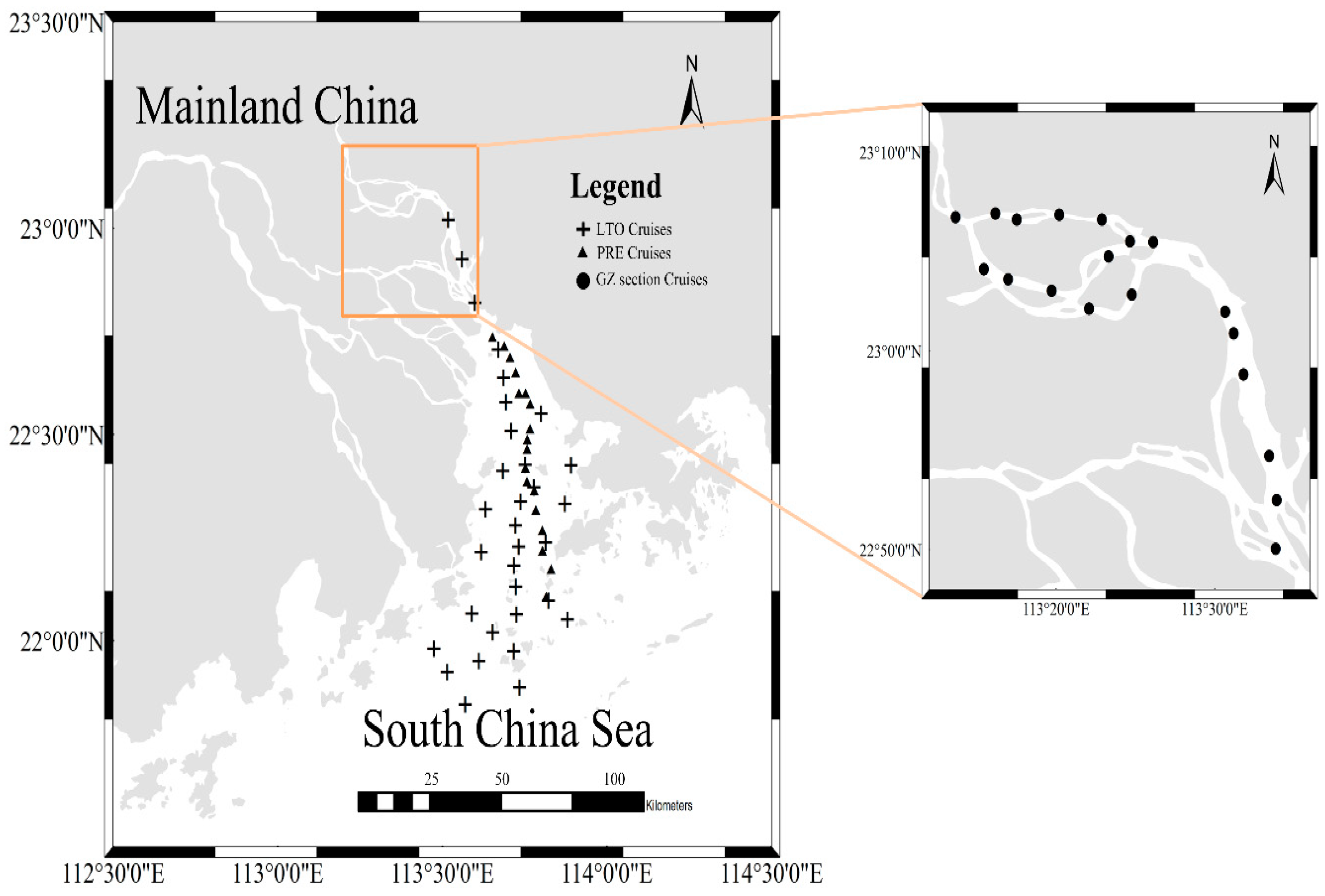
We used an in situ measurement dataset that was collected along three cruise routes. The Pearl River Estuary cruises included 8 cruises from 2003 to 2014, with 16 stations measured during each cruise. The dates of the cruises are 15 January 2003, 1 April 2004, 23 May 2006, 6 December 2006, 15 October 2010, 10 March 2011, 10 December 2012, and 10 September 2014, respectively. These cruises covered the stations in the Pearl River Estuary. The Guangzhou Section cruises included 5 cruises from 2011 to 2014. The dates of the cruises are 7 November 2011, 7 September 2012, 12 December 2012, 17 January 2013, and 25 November 2014, respectively. Measurements were collected during both the wet season and the dry season during the cruises. Finally, the State Key Laboratory of Tropical Oceanography (LTO) cruise was carried out from 4 October to 11 October 2013, and covered more widely distributed stations in the Pearl River Estuary (Figure 2). The measurements covered 258 stations, with synchronous measurements of the suspended sediment concentration and the above water optical data.

The remote sensing reflectance (R_rs) was measured according to the methods of the SeaWiFS project protocol and its further revisions [24,25]. The geometric setup of the radiometric instrument was described by Hooker et al. [26].

The total suspended matter (TSM) concentration was measured by the weighting method. Water samples were filtered onto 47 mm 0.2 μm membrane filters, rinsed with distilled water, and kept frozen until later processing in the laboratory. After thawing, the filters were dried at 60 °C for 24 h and then weighed using a METTLER TOLEDO balance with a precision of 1 μg. The difference between the weights of the filters before and after drying divided by the filtered volume yielded the TSM concentration.

2.2. Satellite Data

The satellite data used in this research included Landsat TM, ETM+, and OLI data. The time spans of the Landsat TM, ETM+, and OLI data were from July 1998 to September 2011, October 1999 to February 2015, and October 2013 to February 2015, respectively. The processed data in these regions included a total of 194 scenes.

The Landsat TM, ETM+, and OLI sensors have three very similar bands in the visible portion of the spectrum, which are located at red, green, and blue, and two similar bands at shortwave infrared (SWIR) wavelengths. The sensors also have one consistent near-infrared (NIR) band. However, the locations of the NIR bands are very different between the TM, ETM+, and OLI sensors (

Table 1. The spectra of the three Landsat TM, ETM+, and OLI sensors (band setting is from http://landsat.usgs.gov/instructions.php, (accessed on 30 September 2020)).

Landsat-8 OLI	Wavelength (μm)	Landsat-7 ETM+	Wavelength (μm)	Landsat-5 TM	Wavelength (μm)
Band 1	0.435–0.450	Band 1 (blue)	0.442–0.513	Band 1 (blue)	0.453–0.517
Band 2 (blue)	0.453–0.512	Band 2 (green)	0.520–0.600	Band 2 (green)	0.529–0.609
Band 3 (green)	0.533–0.590	Band 3 (red)	0.631–0.692	Band 3 (red)	0.627–0.693
Band 4 (red)	0.636–0.673	Band 4	0.772–0.898	Band 4	0.777–0.904
Band 5	0.851–0.878	Band 5	1.55–1.75	Band 5	1.57–1.78
Band 6	1.57–1.65	Band 7	2.07–2.34	Band 7	2.10–2.35
Band 7	2.11–2.29	Band 8	0.516–0.894
Band 8	0.504–0.675
Band 9	1.36–1.38

).

To obtain a spatially continuous distribution of the suspended sediment concentration, a kriging interpolation method was used to remove the stripes from the suspended sediment data in the Landsat ETM+ images.

2.3. Atmospheric Correction of Landsat Data

We used the atmospheric correction method developed in earlier research, which was named the SWIRE (shortwave infrared extrapolation) method [23]. This method was developed based on shortwave infrared (SWIR) to remove aerosol scattering from MODIS data. Compared with other atmospheric correction methods, the SWIRE method used the SWIR bands to remove the reflectance of suspended sediments from the NIR bands. The data provided by the SWIRE method in highly turbid waters were more valid than the data provided by the standard NIR atmospheric correction algorithms. The Rayleigh scattering of the images was firstly removed using the second simulation of a satellite signal in the solar spectrum model [23,27]. Then, the SWIRE method was used to remove the aerosol scattering.

2.4. Symbolic Regression for Algorithm Development

Remote sensing has been widely used to estimate suspended sediment concentrations [16,19,20,28,29]. However, it was unknown if these algorithms had been applied to the Pearl River Estuary. Some algorithms had been developed in the Pearl River Estuary to derive the TSM concentration, but they were not applicable for Landsat data [30,31]. The spectral response function of Landsat was significantly different from these sensors, so it was necessary to re-establish the suspended sediment concentrations algorithm for Landsat in this region. In this study, we developed an explicit suspended sediment concentrations algorithm using symbolic regression.

Symbolic regression is a type of regression method used to search the space of mathematical expressions while minimizing various error metrics based on genetic programming. Symbolic regression is similar to parametric regression, except that the latter requires a given concrete function form, while the former can simultaneously determine the forms of the mathematical expressions and their coefficients using algebraic operators. Generally, symbolic regression obtains the mathematical forms and constants of the coefficients. Therefore, unlike parameter regression, symbolic regression avoids imposing a function from the experiments, and it can be helpful in discovering the underlying mathematical relationships between the target variables and the input variables from a finite number of samples. Of course, the method has the disadvantage of having to search large spaces to identify the functions. In fact, the number of models is generally infinite, which means that symbolic regression will take more time to find a suitable function form and parameterization. Symbolic regression can obtain explicit functions, which may be more efficient for the retrieval of dependent variables than artificial intelligence algorithms, such as support vector machines (SVMs). There is generally no difference in efficiency between the algorithms developed by symbolic regression, and symbolic regression has been used in different studies, including remote sensing and ocean color detection researches [32,33,34,35].

The TSM algorithms were developed using Eureqa software version 1.01.0 in this study. Eureqa is a mathematical software tool originally developed by Michael Schmidt and Hod Lipson in 2009 [36]. The input variables were the in situ remote sensing reflectance values of the three visible bands, and the output variable was the log10-transformed TSM concentrations. The algorithm optimization was stopped when the validation error was no longer improved (new functions would be found) compared to the error from the previous search.

2.5. Band Shift between Landsat TM, ETM+, and OLI

The band settings and their relative spectral responses (RSRs) for the three Landsat sensors were slightly different. The algorithms were developed based on the TM channel setting. We used a simple relationship to shift the spectral parameters for the target blue, green, and red bands for both ETM+ and OLI. The relationship was developed based on 258 groups of optical measurements from the Pearl River dataset, which is sufficient to derive several simple relationships that can be used to shift spectral parameters to the target wavelengths. In this respect, we used an exponential function $y=a{x}^b$ to shift the ETM+ and OLI bands to TM bands. Where y was the Rrs (unit: sr⁻¹) of target bands and x was the Rrs of TM bands. We established 6 equations, and the results are shown in

Table 2. The regression results between the bands of Landsat TM with ETM+ and OLI. The a, b are the fitting coefficients, and R² is the square of the correlation coefficient.

Bands	ETM+			OLI
	a	b	R2	a	b	R2
Blue	1.051	1.006	0.9993	1.009	0.9972	0.9998
Green	1.042	1.012	0.9973	1.037	1.019	0.9957
Red	0.9929	0.9961	0.9999	0.999	0.9956	0.9997

.

3. Results

3.1. Algorithms for Retrieval of Suspended Sediment Concentrations

The in situ suspended sediment concentrations (the TSM concentrations) ranged from 0.52 g m⁻³ to 140 g m⁻³ in the Pearl River, and 4.57 g m⁻³ to 54.73 g m⁻³ in Guangzhou Section. The average values of suspended sediment concentration were 22.68 g m⁻³, 29.52 g m⁻³, 25.02 g m⁻³, and 21.81 g m⁻³ in spring, summer, autumn, and winter. The highest and lowest levels of suspended sediment were observed in the northwest side and in the southeast side, respectively.

The in situ remote sensing reflectance (Rrs) and TSM data were used to develop the TSM retrieval algorithm using the method of Symbolic regression. After training, we obtained the following equations for the retrieval of the TSM concentration,

$$Lo{g}_{10}\left(tsm\right)=0.883+16.24\times R_{rs}\left(red\right)$$

(1)

$$Lo{g}_{10}\left(tsm\right)=1.291+63.85\times R_{rs}\left(red\right)-50.46\times R_{rs}\left(green\right)$$

(2)

$$Lo{g}_{10}\left(tsm\right)=1.918+52.28\times R_{rs}\left(red\right)-0.006455/R_{rs}\left(red\right)-51.35\times R_{rs}\left(green\right)$$

(3)

$$Lo{g}_{10}\left(tsm\right)=\left(0.0009155+2.443\times R_{rs}\left(red\right)\right)/R_{rs}\left(green\right)-0.6735$$

(4)

$$Lo{g}_{10}\left(tsm\right)=2.31+28.41\times R_{rs}\left(red\right)-0.7448\times R_{rs}\left(green\right)/R_{rs}\left(red\right)-23.59\times R_{rs}\left(green\right)$$

(5)

$$Lo{g}_{10}\left(tsm\right)=2.147+35.83\times R_{rs}\left(blue\right)+34.8\times R_{rs}\left(red\right)-0.9546\times R_{rs}\left(blue\right)/R_{rs}\left(red\right)-51.68\times R_{rs}\left(green\right)$$

(6)

$$Lo{g}_{10}\left(tsm\right)=1.454+57.03\times R_{rs}\left(blue\right)+20.19\times R_{rs}\left(red\right)-0.7845\times R_{rs}\left(green\right)/R_{rs}\left(red\right)+\left(0.4927\times R_{rs}\left(red\right)-0.0006733\right)/R_{rs}\left(blue\right)-54.75\times R_{rs}\left(green\right)$$

(7)

where $Lo{g}_{10}\left(tsm\right)$ was the log10-transformed TSM (unit: g m⁻³), and $R_{rs}\left(blue\right)$, $R_{rs}\left(green\right),$ and $R_{rs}\left(red\right)$ were the remote sensing reflectance values (unit: sr⁻¹) of the blue, green, and red bands, respectively.

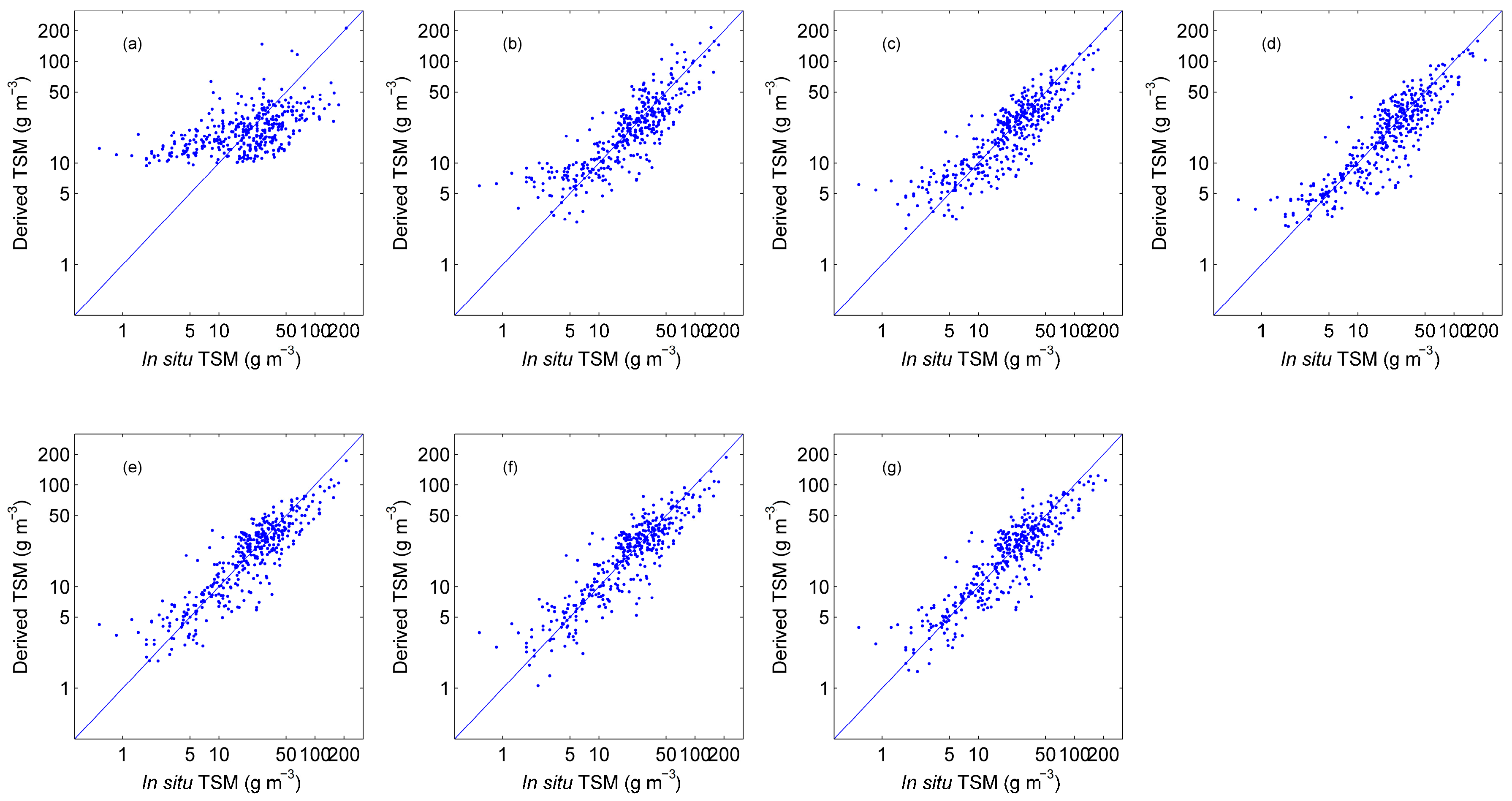
Although the forms of these equations differed, some of them showed very similar results in terms of precision, as indicated in

Table 3. The precisions of the different algorithms used to estimate the TSM concentrations in the Pearl River Estuary. MRE represents mean relative error, MARE represents mean absolute relative error, RMSE represents the root mean squared error (g m⁻³), r represents correlation coefficient, LMAE represents mean absolute error (g m⁻³) in log-10 space, and LRMSE and Lr represent RMSE and r in log-10 space, respectively.

Equation	MRE	MARE	RMSE	r	LMAE	LRMSE	Lr
(1)	63.67	104.7	24.78	0.5078	0.2954	0.3665	0.5507
(2)	22.45	50.22	30.82	0.7266	0.1751	0.2334	0.8438
(3)	15.13	44.27	13.30	0.8860	0.1665	0.2174	0.8660
(4)	7.476	37.78	14.21	0.8664	0.1560	0.2084	0.8791
(5)	8.850	37.54	14.41	0.8749	0.1521	0.2005	0.8872
(6)	10.12	36.88	13.91	0.8741	0.1483	0.1971	0.8917
(7)	8.895	36.20	14.60	0.8618	0.1463	0.1968	0.8920

. It was clear that the improvements from Equations (4) to Equation (7) were limited, which hinted that the form of the retrieved suspended sediment concentration from remote sensing data was not unique. We used Equations (4) to Equation (7) to retrieve the suspended sediment concentration of the Pearl River. We chose one Landsat 8 OLI scene acquired on 16 September 2014 as an example. The results showed very similar suspended sediment distributions in the study area (Figure 3). All of the algorithms demonstrated the suspended sediment pattern in the Pearl River Estuary, which was higher in the northwest and lower in the southeast. However, Equations (7) and Equation (6) showed a significant suspended sediment concentration front from the northwest to the southeast. These two algorithms can obtain better results at lower suspended sediment levels, which can also be seen in the scatter plot in Figure 4. We ultimately selected Equation (7), which performed the best, to retrieve the suspended sediment concentrations in the Pearl River Estuary in terms of the log-10 space.

3.2. Variation in the Suspended Sediment Concentrations after Sand Excavation

To assess the variation in the suspended sediment concentrations due to sand excavation in this area, we divided the images into two categories. One category was with weak or no sand excavation activity, and the other was with strong excavation activity. According to the strategy of the government, before 2013, sand excavation activities to the north of Neilingding Island were rare because sand excavation had not been approved in this region. Since 2013, some companies have been authorized by the local government to excavate sand. As a result, the sand excavation activity increased after 2013. During traditional Chinese holidays, such as the spring festival, the excavation activity was also weak. We defined the times before 2013 and the Chinese spring festival dates as weak/no sand excavation time. The other times were defined as strong sand excavation time.

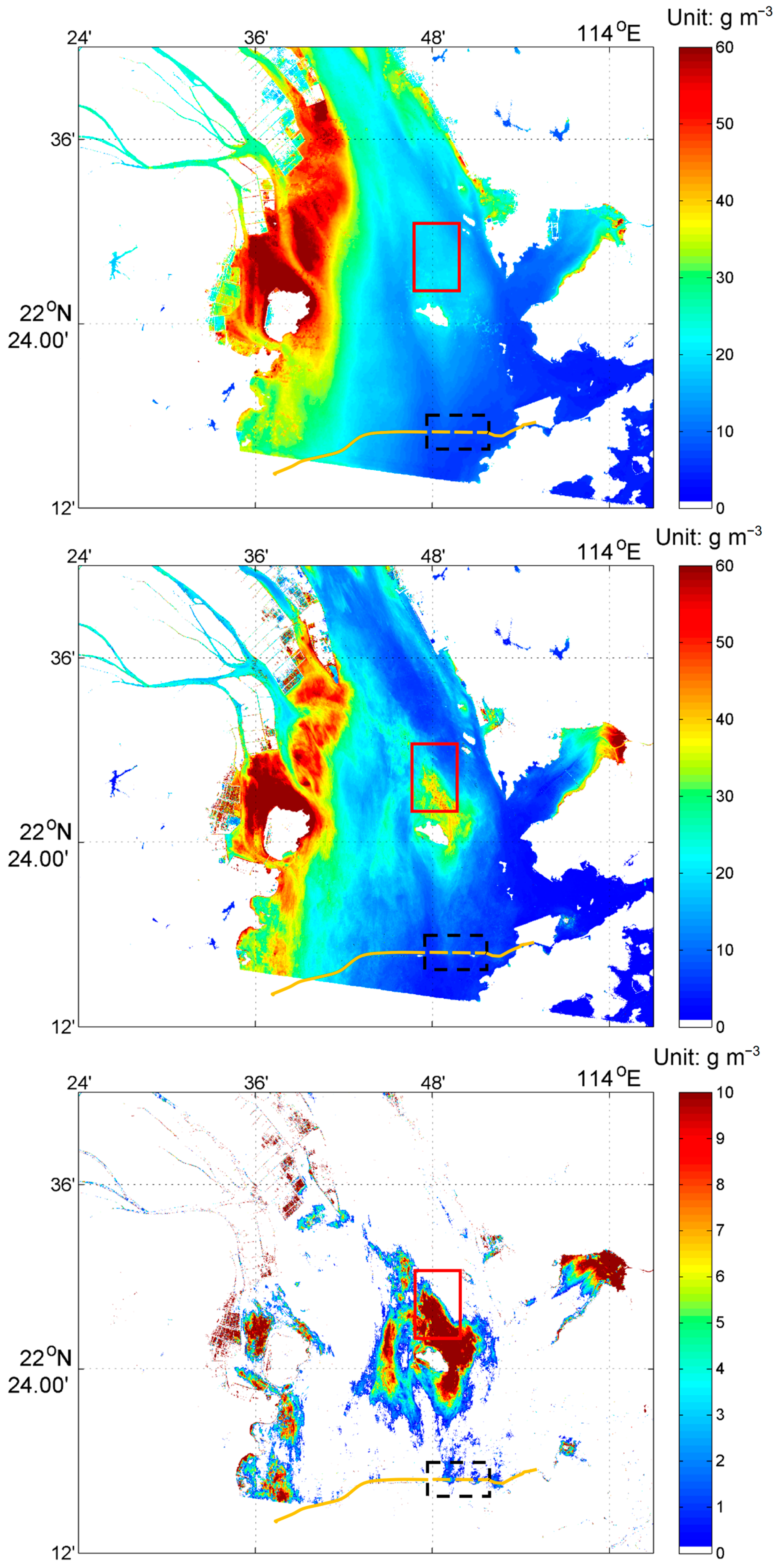
We calculated the average suspended sediment concentrations during the weak/no sand excavation periods, which was regarded as the basic TSM concentrations in these regions. We used the difference between the TSM concentrations during the strong sand excavation period and the averaged TSM concentrations to assess the variation in suspended sediment after strong sand excavation.

It was clear that the increase in suspended sediment around Neilingding Island was significant because of sand excavation. However, the increase in suspended sediment was not spatially contiguous to the area near the Hong Kong-Zhuhai-Macau Bridge tunnel (Figure 5). It was obvious that the TSM concentrations did not show a continuous increase from the region of sand excavation to the tunnel construction region. There was a small increase in suspended sediment in the tunnel region, which seemed to be induced by local construction and not sand excavation in the northern region.

3.3. Correlation Analysis in Different Regions During the Strong/Weak Sand Excavation Periods

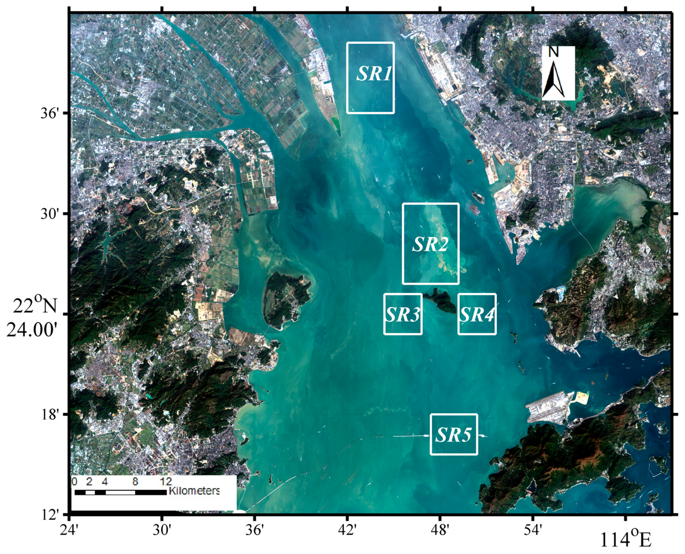
We analyzed the relationship of the time series of the TSM concentrations between different regions before and after sand excavation. We extracted the TSM concentrations in five subregions from the study area (Figure 6). Subregion 1 was located in the north of the estuary, which represented the suspended sediment concentration transported from northern areas; subregion 2 was located in the sand mining area, which represented the high TSM concentrations induced by sand excavation; subregion 3 and subregion 4 were located on the west and east sides of Neilingding Island, respectively, and represented the southern region near the sand excavation area, where the TSM concentrations were affected by sand excavation activities; subregion 5 was the Hong Kong-Zhuhai-Macau Bridge construction zone, where we analyzed whether or not the TSM concentrations were influenced by the sand excavation activities.

A correlation analysis was employed to detect the relationship between the time series of the averaged TSM concentration in the different subregions. As shown in

Table 4. The correlation coefficient of the TSM concentrations in different subregions (all images). SR1 represents subregion 1, SR2 represents subregion 2, etc. All the correlation coefficients passed the significance test (N = 194, p < 0.01).

R2	SR2	SR3	SR4	SR5
SR1	0.604	0.449	0.575	0.367
SR2	-	0.764	0.712	0.525
SR3	-	-	0.567	0.658
SR4	-	-	-	0.543

, throughout the study period, if two subregions were closer, the R² value was high. As an example, SR2 showed high correlation coefficients of 0.764 and 0.712 with SR3 and SR4, respectively. SR1 showed the lowest correlation coefficient with SR5, which was only 0.367.

To evaluate the variability of the correlation coefficients after sand excavation, the data were divided into two periods according to the occurrence of sand excavation (

Table 5. The correlation coefficient (R²) of the TSM concentrations between SR2 and other subregions during the strong excavation period and the weak/no excavation period. All the correlation coefficients passed the significance test (p < 0.01).

TSM of Subregions	TSM of SR2
	Strong Excavation Period	Weak/No Excavation Period
SR1	0.433	0.631
SR3	0.768	0.753
SR4	0.714	0.706
SR5	0.487	0.509

). The correlation coefficient between SR1 and SR2 decreased during the strong excavation period, which meant that the background suspended sediment concentrations had a smaller impact on SR2 during the strong excavation period because the variability of the suspended sediment concentrations in SR2 was mostly influenced by the excavation activities in the region. The correlation coefficient between SR2 and SR3 did not show significant changes during the two periods, which meant that the impact of the suspended sediment concentrations of SR2 on SR3 did not change substantially after sand excavation. Sand excavation did not change the co-variation between SR2 and SR3, indicating that the impact of the sand excavation in SR2 on SR3 may be similar to the impact from the background suspended sediment concentrations (the suspended sediment concentrations of SR2 without sand excavation). Both SR4 and SR3 exhibited similar correlation with SR2. The correlation coefficient between SR2 and SR5 decreased during the strong excavation period, which indicated that the suspended sediment concentration related to sand excavation had less impact on SR5 than the background suspended sediment concentration. Thus the main factor in the suspended sediment variability in SR5 was not sand excavation activities.

4. Discussion

Satellite remote sensing is a useful method for analyzing the variability in suspended sediment concentrations in the open ocean. In coastal waters, satellite remote sensing experiences some difficulties because of atmospheric correction, algorithm development and the limited spatial resolution of some sensors. However, in coastal regions, the signal reflected from the water is generally stronger than that reflected from open waters. As a result, satellite sensors designed for land surveys, such as Landsat, may have difficulty detecting color in open waters, but they can successfully detect water quality in river and coastal regions [37,38].

Suspended sediment is a very important parameter for water quality detection, port engineering construction, the fishing industry and aquaculture farms. The detection of suspended sediment concentrations in coastal regions is still challenging. At present, there is no widely accepted remote sensing product that can be used for suspended sediment estimations in all coastal regions. Most remote sensing retrievals of TSM concentrations have been based on empirical relationships between in situ remote sensing reflectance values and TSM concentrations [39,40]. The relationship between remote sensing reflectance values and TSM concentrations is generally uncertain. Regular data fitting methods only calculate coefficients based on some simple expressions, such as a linear or exponential equation [41]. Symbolic regression methods can simultaneously determine the forms of the mathematical expressions and their coefficients using algebraic operators. This study acquired seven algorithms for the retrieval of suspended sediment information. These algorithms showed a significant diversity in terms of their forms. Some of these algorithms showed a slightly different precision, which demonstrated that the explicit algorithms to estimate suspended sediment concentrations were not unique. The algorithms might have significant physical meanings, such as in Equation (4), which was very similar to the remote sensing reflectance ratio between red and green bands. Similar band ratio algorithms had been reported in previous studies [42]. The TSM concentrations had a robust relationship with the remote sensing reflectance values in the visible portion of the spectrum, and some studies had indicated that combining red reflectance values with reflectance values in one or more other visible bands could increase the robustness [43], which was consistent with our results. In addition, a large amount of in situ data was used to develop the TSM algorithm in this study, yielding a more robust relationship between the remote sensing reflectance values and the TSM concentrations.

Although some remote sensing studies of suspended sediment concentrations had been reported in the literature [13,15,28,30], limited research had been conducted on the connection between regional correlations of satellite-derived TSM concentrations and the construction of infrastructure and buildings. Due to complicated and dynamic estuarine processes, the large number of high-resolution satellite images was beneficial to identify the intrinsic connection. In this study, 194 Landsat satellite images were used to analyze the impact of sand excavation on the suspended sediment concentrations in the Hong Kong-Zhuhai-Macau Bridge region, which provided a more reliable conclusion. In addition, Landsat images exhibited a much higher spatial resolution than ocean color satellite images, which provided a fine-scale (~10 meters spatial resolution) distribution and decreased the impact of adjacent non-water body reflectance on water body pixels. The study did not consider bottom reflectance. The remotely sensed TSM concentrations were derived from the information of the first attenuation depth, which is the depth at which light is attenuated by approximately 10% of the surface light irradiance. The settlement speed of suspended sediment differed for different particle sizes. The settlement velocity of suspended sediment may have some impact on the correlation analysis between different subregions. However, in this study, the distance between different subregions was relatively small, especially for the sand excavation-affected subregion and the infrastructure construction subregion. Thus, it could be assumed that the background settlement velocity of the suspended sediment was similar.

5. Conclusions

Sand is one of the most important aggregate materials for the construction of infrastructure and buildings. With the development of the economy, sand mining activities in rivers have become universal, especially in some East and Southeast Asian countries, where sand excavation has been reported to impact the river environments [44,45,46]. However, adequate information on the effects of sand excavation on the environment is still lacking, which poses challenges to regulation and management [47]. Based on years of field observations in the Pearl River Estuary, this study developed models to assess the suspended sediment concentrations in the Pearl River Estuary using Landsat satellites. The models were established using symbolic regression based on genetic programming. After using the SWIRE algorithm for atmospheric correction, Landsat satellite data were processed, and 194 time series of suspended sediment concentrations in the Pearl River Estuary were produced. Then, the variation in the suspended sediment concentrations at the surface near the Hong Kong-Zhuhai-Macau Bridge tunnel construction region before and after sand excavation activities was illustrated. The results showed that there was no significant variability in the TSM concentrations in the tunnel construction region because of the sand excavation in the northern area.

References

- Harrison, P.J.; Yin, K.D.; Lee, J.H.W.; Gan, J.P.; Liu, H.B. Physical–biological coupling in the pearl river estuary. Cont. Shelf Res. 2008, 28, 1405–1415. [Google Scholar] [CrossRef]
- Wu, C.; Ji, C.; Shi, B.; Wang, Y.; Gao, J.; Yang, Y.; Mu, J. The impact of climate change and human activities on streamflow and sediment load in the Pearl River basin. Int. J. Sediment Res. 2019, 34, 307–321. [Google Scholar] [CrossRef]
- Hu, J.T.; Li, S.Y.; Geng, B.X. Modeling the mass flux budgets of water and suspended sediments for the river network and estuary in the Pearl River Delta, China. J. Mar. Syst. 2011, 88, 252–266. [Google Scholar] [CrossRef]
- Mao, Q.; Shi, P.; Yin, K.; Gan, J.; Qi, Y. Tides and tidal currents in the Pearl River Estuary. Cont. Shelf Res. 2004, 24, 1797–1808. [Google Scholar] [CrossRef]
- Dong, L.; Su, J.; Li, Y.; Xia, X.; Guan, W. Physical processes and sediment dynamics in the Pearl River. In The Environment in Asia Pacific Harbours; Wolanski, E., Ed.; Springer: Dordrecht, The Netherlands, 2006; pp. 127–137. [Google Scholar]
- Luo, X.L.; Zeng, E.Y.; Ji, R.Y.; Wang, C.P. Effects of in-channel sand excavation on the hydrology of the Pearl River Delta, China. J. Hydrol. 2007, 343, 230–239. [Google Scholar] [CrossRef]
- Padmalal, D.; Maya, K. Impacts of River Sand Mining. In Sand Mining: Environmental Impacts and Selected Case Studies; Springer: Dordrecht, The Netherlands, 2014; pp. 31–56. [Google Scholar]
- Wei, G.; Qiu, H.J.; Wang, D.D. Study of sedimentation speed and compression characteristics of back-silting soil from undersea immersed tube tunnels. Appl. Mech. Mater. 2014, 501–504, 132–136. [Google Scholar] [CrossRef]
- Blondeau-Patissier, D.; Gower, J.F.R.; Dekker, A.G.; Phinn, S.R.; Brando, V.E. A review of ocean color remote sensing methods and statistical techniques for the detection, mapping and analysis of phytoplankton blooms in coastal and open oceans. Prog. Oceanogr. 2014, 123, 123–144. [Google Scholar] [CrossRef] [Green Version]
- Carder, K.L.; Steward, R.G.; Paul, J.H.; Vargo, G.A. Relationships between chlorophyll and ocean color constituents as they affect remote-sensing reflectance models. Limnol. Oceanogr. 1986, 31, 403–412. [Google Scholar] [CrossRef]
- Chen, C.Q.; Shi, P.; Zhan, H.G. A local algorithm for estimation of yellow substance (gelbstoff) in coastal waters from SeaWiFS data: Pearl River Estuary, China. Int. J. Remote Sens. 2003, 24, 1171–1176. [Google Scholar] [CrossRef]
- Liu, F.F.; Tang, S.L. Evaluation of Red-Peak Algorithms for Chlorophyll Measurement in the Pearl River Estuary. IEEE Trans. Geosci. Remote Sens. 2019. [Google Scholar] [CrossRef]
- Tang, S.L.; Larouche, P.; Niemi, A.; Michel, C. Regional algorithms for remote-sensing estimates of total suspended matter in the Beaufort Sea. Int. J. Remote Sens. 2013, 34, 6562–6576. [Google Scholar] [CrossRef]
- Chen, C.Q.; Tang, S.L.; Pan, Z.L.; Zhan, H.G.; Larson, M.; Jonsson, L. Remotely sensed assessment of water quality levels in the Pearl River Estuary, China. Mar. Pollut. Bull. 2007, 54, 1267–1272. [Google Scholar] [CrossRef] [PubMed]
- Hu, C.M.; Chen, Z.Q.; Clayton, T.D.; Swarzenski, P.; Brock, J.C.; Muller-Karger, F.E. Assessment of estuarine water-quality indicators using MODIS medium-resolution bands: Initial results from Tampa Bay, FL. Remote Sens. Environ. 2004, 93, 423–441. [Google Scholar] [CrossRef]
- Brando, V.E.; Dekker, A.G. Satellite hyperspectral remote sensing for estimating estuarine and coastal water quality. IEEE Trans. Geosci. Remote Sens. 2003, 41, 1378–1387. [Google Scholar] [CrossRef]
- Maritorena, S.; Siegel, D.A.; Peterson, A.R. Optimization of a semianalytical ocean color model for global-scale applications. Appl. Opt. 2002, 41, 2705–2714. [Google Scholar] [CrossRef] [PubMed]
- Gilvear, D.; Tyler, A.; Davids, C. Detection of estuarine and tidal river hydromorphology using hyper-spectral and LiDAR data: Forth estuary, Scotland. Estuar. Coast. Shelf Sci. 2004, 61, 379–392. [Google Scholar] [CrossRef]
- Dorji, P.; Fearns, P. A quantitative comparison of total suspended sediment algorithms: A case study of the last decade for MODIS and landsat-based sensors. Remote Sens. 2016, 8, 810. [Google Scholar] [CrossRef] [Green Version]
- Peterson, K.T.; Sagan, V.; Sidike, P.; Cox, A.L.; Martinez, M. Suspended sediment concentration estimation from landsat imagery along the lower Missouri and Middle Mississippi Rivers using an extreme learning machine. Remote Sens. 2018, 10, 1503. [Google Scholar] [CrossRef] [Green Version]
- Wang, M.H. Remote sensing of the ocean contributions from ultraviolet to near-infrared using the shortwave infrared bands: Simulations. Appl. Opt. 2007, 46, 1535–1547. [Google Scholar] [CrossRef]
- Wang, M.H.; Shi, W. The NIR-SWIR combined atmospheric correction approach for MODIS ocean color data processing. Opt. Express 2007, 15, 15722–15733. [Google Scholar] [CrossRef] [PubMed] [Green Version]
- Ye, H.B.; Chen, C.Q.; Yang, C.Y. Atmospheric correction of landsat-8/OLI Imagery in turbid estuarine waters: A case study for the Pearl River Estuary. IEEE J. Sel. Top. Appl. Earth Obs. Remote Sens. 2017, 10, 252–261. [Google Scholar] [CrossRef]
- Mueller, L.J. Ocean optics protocols for satellite ocean color sensor validation. In Biogeochemical and Bio-Optical Measurements and Data Analysis Protocols, 5th ed.; NASA: Greenbelt, MD, USA, 2003; Volume V, pp. 1–30. [Google Scholar]
- Mueller, J.L. Ocean optics protocols for SeaWiFS validation. In NASA Tech. Memo 104566, 1st ed.; NASA Goddard Space Flight Center: Greenbelt, MD, USA, 1992; pp. 1–69. [Google Scholar]
- Hooker, S.B. The seaBOARR-98 field campaign. In NASA Technical Memorandum 1999-206892; NASA Goddard Space Flight Center: Greenbelt, MD, USA, 2000; pp. 1–40. [Google Scholar]
- Vermote, E.F.; Tanre, D.; Deuze, J.L.; Herman, M.; Morcette, J. Second simulation of the satellite signal in the solar spectrum, 6S: An overview. IEEE Trans. Geosci. Remote Sens. 1997, 35, 675–686. [Google Scholar] [CrossRef] [Green Version]
- Li, R.; Kaufman, Y.J.; Gao, B.; Davis, C.O. Remote sensing of suspended sediments and shallow coastal waters. IEEE Trans. Geosci. Remote Sens. 2003, 41, 559–566. [Google Scholar]
- Tian, L.Q.; Wai, O.W.H.; Chen, X.L.; Liu, Y.H.; Feng, L.; Li, J.; Huang, J. Assessment of total suspended sediment distribution under varying tidal conditions in deep bay: Initial results from HJ-1A/1B satellite CCD images. Remote Sens. 2014, 6, 9911–9929. [Google Scholar] [CrossRef] [Green Version]
- Xing, Q.; Lou, M.; Chen, C.; Shi, P. Using in situ and satellite hyperspectral data to estimate the surface suspended sediments concentrations in the Pearl River estuary. IEEE J. Sel. Top. Appl. Earth Obs. Remote Sens. 2013, 6, 731–738. [Google Scholar] [CrossRef]
- Xi, H.; Zhang, Y. Total suspended matter observation in the Pearl River estuary from in situ and MERIS data. Environ. Monit. Assess. 2011, 177, 563–574. [Google Scholar] [CrossRef]
- Chami, M.; Robilliard, D. Inversion of oceanic constituents in case I and II waters with genetic programming algorithms. Appl. Opt. 2002, 41, 6260–6275. [Google Scholar] [CrossRef]
- Chang, C.-H. Development of ocean color algorithms for estimating chlorophyll-a concentrations and inherent optical properties using gene expression programming (GEP). Opt. Express 2015, 23, 5417–5437. [Google Scholar] [CrossRef]
- Fonlupt, C. Solving the ocean color problem using a genetic programming approach. Appl. Soft Comput. 2001, 1, 63–72. [Google Scholar] [CrossRef]
- Tang, S.; Michel, C.; Larouche, P. Development of an explicit algorithm for remote sensing estimation of chlorophyll a using symbolic regression. Opt. Lett. 2012, 37, 3165–3167. [Google Scholar] [CrossRef]
- Schmidt, M.; Lipson, H. Distilling free-form natural laws from experimental data. Science 2009, 324, 81–85. [Google Scholar] [CrossRef] [PubMed]
- Manzo, C.; Braga, F.; Zaggia, L.; Brando, V.E.; Giardino, C.; Bresciani, M.; Bassani, C. Spatio-temporal analysis of prodelta dynamics by means of new satellite generation: The case of Po river by Landsat-8 data. Int. J. Appl. Earth Obs. Geoinf. 2018, 66, 210–225. [Google Scholar] [CrossRef]
- Zhang, M.W.; Dong, Q.; Cui, T.W.; Xue, C.J.; Zhang, S.L. Suspended sediment monitoring and assessment for Yellow River estuary from Landsat TM and ETM+ imagery. Remote Sens. Environ. 2014, 146, 136–147. [Google Scholar] [CrossRef]
- Wang, J.J.; Lu, X.X.; Liew, S.C.; Zhou, Y. Remote sensing of suspended sediment concentrations of large rivers using multi-temporal MODIS images: An example in the Middle and Lower Yangtze River, China. Int. J. Remote Sens. 2010, 31, 1103–1111. [Google Scholar] [CrossRef]
- Song, K.; Dongmei, L.; Liu, D.; Wang, Z.; Li, L.; Zhang, B.; Wang, Y. In Retrival of total suspended matter (TSM) using remotely sensed images in Shitoukoumen Reservior, Northeast China. In Proceedings of the 2010 IEEE International Geoscience and Remote Sensing Symposium, Honolulu, HI, USA, 25–30 July 2010; pp. 405–408. [Google Scholar]
- Wang, F.; Zhou, B.; Liu, X.; Zhou, G.; Zhao, K. Remote-sensing inversion model of surface water suspended sediment concentration based on in situ measured spectrum in Hangzhou Bay, China. Environ. Earth Sci. 2012, 67, 1669–1677. [Google Scholar] [CrossRef]
- Doxaran, D.; Froidefond, J.-M.; Lavender, S.; Castaing, P. Spectral signature of highly turbid waters: Application with SPOT data to quantify suspended particulate matter concentrations. Remote Sens. Environ. 2002, 81, 149–161. [Google Scholar] [CrossRef]
- Binding, C.E.; Bowers, D.G.; Mitchelson-Jacob, E.G. Estimating suspended sediment concentrations from ocean colour measurements in moderately turbid waters; the impact of variable particle scattering properties. Remote Sens. Environ. 2005, 94, 373–383. [Google Scholar] [CrossRef]
- Brunier, G.; Anthony, E.J.; Goichot, M.; Provansal, M.; Dussouillez, P. Recent morphological changes in the Mekong and Bassac river channels, Mekong delta: The marked impact of river-bed mining and implications for delta destabilisation. Geomorphology 2014, 224, 177–191. [Google Scholar] [CrossRef]
- Hackney, C.R.; Darby, S.E.; Parsons, D.R.; Leyland, J.; Best, J.L.; Aalto, R.; Nicholas, A.P.; Houseago, R.C. River bank instability from unsustainable sand mining in the lower Mekong River. Nat. Sustain. 2020, 3, 217–225. [Google Scholar] [CrossRef]
- Park, E.; Ho, H.L.; Tran, D.D.; Yang, X.K.; Alcantara, E.; Merino, E.; Son, V.H. Dramatic decrease of flood frequency in the Mekong Delta due to river-bed mining and dyke construction. Sci. Total Environ. 2020, 723, 138066. [Google Scholar] [CrossRef] [PubMed]
- Padmalal, D.; Maya, K. Introduction. In Sand Mining: Environmental Impacts and Selected Case Studies; Springer: Dordrecht, The Netherlands, 2014; pp. 1–7. [Google Scholar]
Figure 1.
A map of the study area. The color is the water area extracted from the true color image of the Landsat-8 data acquired on 3 January 2015. The gray line is the isobath from the GEBCO bathymetric data. The red rectangle is the permitted sand excavation region, and the black rectangle is the tunnel construction area. The solid orange line is the bridge, and the dotted orange line is the undersea tunnel.
Figure 2.
The sample stations of the three cruise routes used in this study; the plus sign represents the LTO cruise stations, the triangles represent the stations of the Pearl River Estuary cruises, and the solid circles represent the stations of Guangzhou Section cruises.
Figure 3.
The suspended sediment distribution derived using different algorithms (Equations (7) to Equation (4)). The scene was captured on 16 November 2014.
Figure 4.
The scatter plots of the derived suspended sediment concentrations and the measured suspended sediment concentrations. The derived total suspended matter (TSM) concentrations in (a–f) and (g) were obtained from Equations (1) to (7), respectively.
Figure 5.
Mean suspended sediment concentrations during the weak/no excavation period (top); mean suspended sediment concentrations during the strong excavation period (middle); the difference between the mean suspended sediment concentrations during the strong excavation period and the weak/no excavation period. The red rectangle is the permitted sand excavation region, and the black rectangle is the tunnel construction area. The solid orange line is the bridge, and the dotted orange line is the undersea tunnel.
Figure 6.
True color image of the Landsat-8 data acquired on 3 January 2015. The five extracted Scheme 1. represents subregion 1, SR2 represents subregion 2, etc. SR2 is the sand excavation area.