
Towards a Solid Particle Hydrodynamic (SPH)-Based Solids Transport Model Applied to Ultra-Low Water Usage Sanitation in Developing Countries


Institute for Sustainable Building Design, Riccarton Campus, Heriot-Watt University, Edinburgh EH14 4AS, UK
*
Author to whom correspondence should be addressed.
Water 2021, 13(4), 441; https://doi.org/10.3390/w13040441
Submission received: 5 January 2021
/
Revised: 2 February 2021
/
Accepted: 4 February 2021
/
Published: 8 February 2021
(This article belongs to the Section Urban Water Management)
Abstract
:Distribution of toilet facilities and low-cost small-bore simplified sewerage systems (SS) in peri-urban areas provide opportunities to improve public health, provide safely managed sanitation, and protect the environment in low-to-middle income countries. Smoothed particle hydrodynamics (SPH) offers opportunities for optimisation of ultra-low water usage systems, but not without computational challenges. Results from SPH modelling of low cost, low water usage sanitary appliances were compared to a validated 1D finite difference model (DRAINET) for evaluation and calibration. An evaluation of system performance linked solid transport capabilities to physical geometries. The SPH model was developed for a pour-flush toilet pan connected to a 100 mm diameter pipe. The scheme utilized a free surface turbulent model to evaluate solid (faecal) transport efficacy. Performance was greatly influenced by the artificial viscosity factor, ViscoBoundFactor, within SPH, relating to the interaction of fluid and fluid particles and fluid and boundary particles. Results indicate that an increase in this factor leads to a reduction in fluid velocity with an attendant reduction in solid transportation distance, leading to inaccuracies. Other issues such as the use of density and mass in the definition of solid characteristics made it less predictable than the established 1D model for predicting solid transport. Overall, SPH was found to be useful for characterising the geometry of the pour flush pan but not for whole system assessment. A hybrid method is thus recommended whereby the design and performance characteristics for the input stage can be modelling in SPH but the whole system pipe network evaluation is better suited to the 1D DRAINET model.
1. Introduction
There are significant benefits from being able to model geometrically accurate appliances and fittings in the water domain. This is no less true for optimizing designs in sanitation provision in developing countries. Ultra-low water usage systems present opportunities to up-scale sanitation provision, however, this is a challenging effort [1]. Modelling whole system performance provides an opportunity to investigate performance of a section of the system, including the pour flush toilet input and the connection pipe to a larger network. This part of the system is where blockages and failures are more likely to occur if the design is not correct. Smoothed particle hydrodynamics (SPH) provides an opportunity to look at the design of this part of the system in order to optimize it. The SPH model presents many challenges in this particular setting, and this paper highlights how a generic 3D model can be adapted and calibrated to more accurately represent the input system to a simplified sewerage system [2].
Previous studies have utilised DRAINET [3], a one dimensional, method of characteristics modelling, utilising a finite difference scheme to establish system performance in a free surface flow context to design a simplified sewerage system for Marikuppam, a small village in India, from which this study is influenced [1]. As DRAINET does not have the capability to deal with complex geometries in a constructive way, smoothed particle hydrodynamic (SPH) provides the opportunity to assess the performance of the system and its geometry.
This paper focused on the calibration of the SPH model by evaluating the effect of certain inputs to SPH on the model performance on the system as shown in Figure 1. No evaluation was completed for DRAINET, since this is a well-developed simulation program whose validation has been dealt with elsewhere [3,4,5,6,7]. The results were compared to output data from the DRAINET model and measured data to determine the effect these inputs have on the system performance, and to allow for conclusions to be drawn. Obtaining this information will allow for further work to take place, including optimisation of the system and ensuring it is suitable for installation with minimal risk of blockage.
DualSPHysics was used as the smooth particle hydrodynamic (SPH) model in the study. DualSPHysics is an open source smoothed particle hydrodynamics (SPH) model, originating from SPHysics code, developed by researchers at the University of Manchester, John Hopkins University, University of Vigo, and University of Rome [8].
SPH originated within astrophysics to provide reasonable accuracy whilst being simple to work with [9,10], where the equations of fluid dynamics replace the fluid with particles, interpolation points, which can then be used to determine properties of the fluid. The particle representation conserves energy, momentum (linear and angular), mass, and entropy (if no artificial viscosity operates), whilst unlike alternative Eulerian mesh-based techniques like Computational Fluid Dynamics (CFD), SPH algorithms are Galilean invariant [11].
SPH is a meshless model that approximates the continuum dynamics of fluid through derivation of the hydrodynamical equations of motion [12]. The modelling of fluid simulations using SPH is based upon the Navier–Stokes equations, defined at each particle location depending on the characteristics of surrounding particles. The properties of fluids or solids are calculated in relation to the particles within the simulations. Particle characteristics are redefined at each new time step, which results in particle movement and new properties. A brief discussion of the modelling techniques employed are given below.
2. Materials and Methods
The overarching methodology employed in this research was to compare and calibrate, where necessary, two different modelling techniques in order to more closely investigate ultra-low water usage devices. The models are an SPH 3D DualSPhysics model and an in-house 1D finite difference model utilizing the method of characteristics for the solution of the St. Venant equations (DRAINET). A brief description of both techniques follows, with particular reference to the artificial viscosity parameter ViscoBoundFactor, since this proved to be problematic during implementation.
2.1. Laboratory Setup
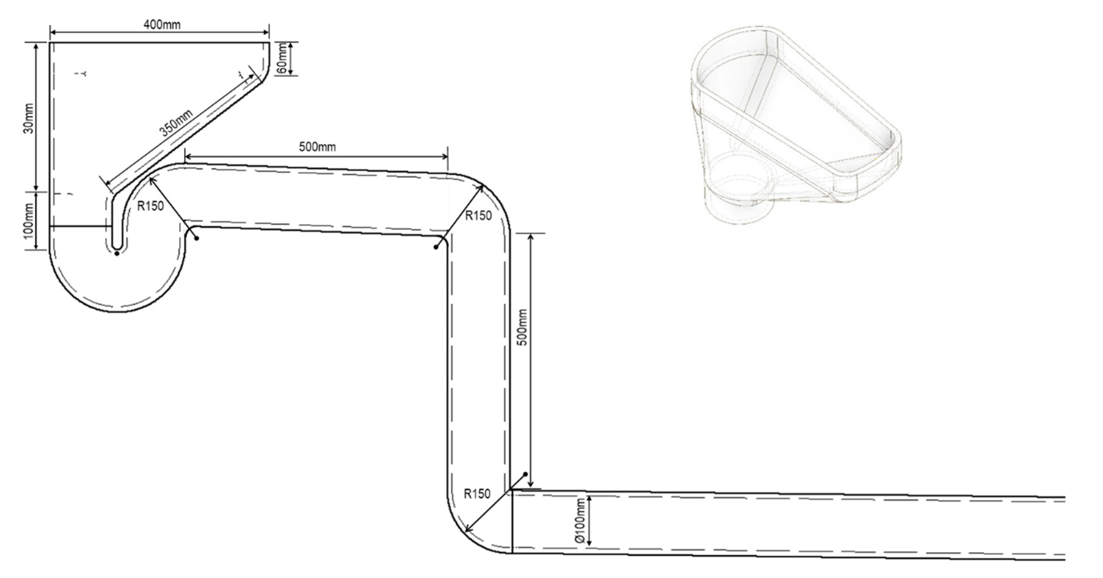
The system under consideration is shown in Figure 1 and represents the part of the system close to people’s dwellings.
The laboratory setup entailed a 100 mm diameter pipe at a 1:100 gradient and was 4 m in length. The setup, with further dimensions, is included in Figure 1. The laboratory experiment was carried out to determine the solid transportation distance for two specific gravity of solids using only 1.3 L of water, which could then be compared with DRAINET and SPH. The quantity of water, 1.3 L, was established from the size of a typical pouring jug used in developing countries in pour flush toilets. One of these standard jugs was utilised in the laboratory setup when water was poured into the system to replicate the pouring of water into a simplified sewerage system.
The solid (80 mm length, 36 mm diameter) was positioned around 1 m into the 10 m long section of pipe. The starting location was recorded, and water was poured into the system and the distance that the solid was transported was noted. This process was repeated until the threshold (4 m from system entry) was reached or when the solid was deposited permanently. This procedure was carried out for solids of two different specific gravity values to determine the maximum transportation of each.
2.2. DualPhysics SPH
SPH is a meshless model that approximates the continuum dynamics of fluid through derivation of the hydrodynamical equations of motion [8,12]. The modelling of fluid simulations using SPH is based upon the Navier–Stokes equations, defined at each particle location depending on the characteristics of surrounding particles. The properties of fluids or solids are calculated in relation to the particles within the simulations. Particle characteristics are redefined at each new time step which results in particle movement and new properties.
2.2.1. Momentum Equation
The momentum equation is a governing equation within SPH, written as:
The dissipative terms, Γ, include viscosity where this can be artificial viscosity or laminar and sub-particle ccale (SPS) viscosity. Viscosity can be influenced by several parameters within DualSPHysics.
Artificial viscosity is most commonly used in SPH simulations [13] due to its simplicity. Including artificial viscosity in the momentum conservation equation, it can be written:
Π is artificial viscosity and ∇aWab is the kernel function with respect to particles a and b.
An execution parameter of DualSPHysics, ViscoTreatment, describes the viscosity based on whether the movement is Artificial (1) or Laminar+SPS (2). This parameter has a default of 1, artificial viscosity.
Cab = 0.5(Ca + Cb) is the mean speed of sound, and α is a coefficient used to introduce energy lost through friction to the case [8]. Alteration of this coefficient, α, adjusts the artificial viscosity, allowing for a more real representation of fluid flow.
The parameter α is used for artificial viscosity, which depends on the smoothing length (h) and the initial distance between particles. ViscoBoundFactor, is a DualSPHysics parameter introduced as a way of defining different values of α. The user guide for DualSPHysics code [8] specifies ViscoBoundFactor as the product of the viscosity and boundary, defaulted as 1, written as:
αFB refers to the interaction between fluid and boundary particles and αFF the interaction between fluid particles [8]. When the ViscoBoundFactor is taken as 1, this suggests the interactions of fluid–fluid and fluid–boundary particles are equal. In a physical environment this is likely to not be the case, with roughness of the material influencing the friction present, and hence adjustment of the ViscoBoundFactor is required to best simulate reality.
As the ViscoBoundFactor is commonly taken as 1, this implies that the interaction of fluid–fluid particles and fluid–boundary particles are equal. As stated by Barreiro [14], this is usually the case in a laboratory set up. In their experiment carried to analyse water flow and runoff as a result of extreme rainfall, Plexiglas was used in the laboratory, which has very little influence on the propagation of water [8]. However, outside of the laboratory, the physical environment is likely to have an impact on the fluid movement due to the roughness of the material, causing the friction to increase. To ensure the correct terrain was simulated on SPH, the ViscoBoundFactor (VBF) was adjusted to obtain a valid flow. From previous research, a possible value for αFF was obtained for the given scenario, and therefore a value for αFB was required to input the ViscoBoundFactor into SPH. For this, the Manning equation was used:
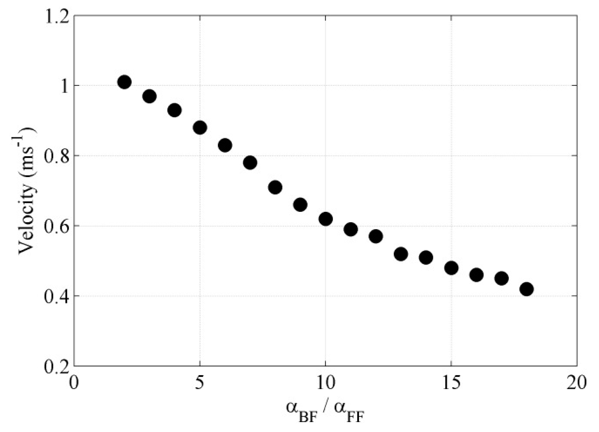
This allows the velocity, v, to be calculated based on the Manning coefficient, n, the hydraulic radius, R, and the channel slope, S. This allowed the predicted velocity for the situation to be determined, where different VBFs were simulated to establish which VBF achieved the correct velocity. This allowed αFB to be established, providing a relationship between flow velocity and VBF, Figure 2.
Figure 2 shows that the VBF has a significant effect on the velocity of the flow with an over 60% reduction in velocity, varying the factor from 1 to 18. The ViscoBoundFactor provides a computed version of roughness [14], which is similarly stated as a factor enabling a “numerical” simulation of roughness [15]. This makes the VBF an important parameter in the simulation of artificial viscosity, and the calibration of the model. With regard to the simplified sewerage model, an attempt was made to calibrate the ViscoBound Factor with data from solid transport from the laboratory investigation and from 1D modelling, however, this was not entirely satisfactory (see below).
2.2.2. Continuity Equation
The Naviar–Stokes continuity equation (or conservation of mass) is defined as:
where ρ is density, t is time, m is mass, v is velocity, and ∇aWab is the kernel function.
In SPH simulations, the mass of particles remains constant over time, however, their density varies [8]. To reduce the fluctuation in density, delta-SPH is introduced as a diffusive term to the continuity equation [10]:
where delta-SPH, δΦ, must be assigned a relevant value. In most situations, the use of a delta-SPH (δΦ) coefficient of 0.1 is deemed appropriate.
2.2.3. Delta-SPH
High frequency, low amplitude oscillations are observed in the density field as a result of the rigid density field from the state equation, and the expected variation of Lagrangian particles. The equation of state determines the fluid pressure depending on particle density based on the fluid in SPH being weakly compressible. To lower the speed of sound, artificially, the compressibility of the fluid can be altered. However, this results in a restriction of the speed of sound to being at least ten times the maximum velocity of the fluid, and the density varies by less than 1%.
Including delta-SPH into the continuity equation, as a diffusive term, results in Equation (7).
2.2.4. Particle Motion
As SPH is a particle-based method of simulation, the particles movement has been defined to keep the velocity of a moving particle close to the average of all moving particles in the vicinity. This results in a more orderly flow of particles, reducing outliers within the flow. The particles are computed according to:
where ε ranges from 0 to 1, defined as a problem specific parameter, m is mass, v is velocity, ρab = 0.5(ρa + ρb), and W is the kernel function.
2.2.5. Processing
The dissipative terms mentioned in the DualSPHysics formulation rely on user input to provide results for the specific situation. These are input during the pre-processing stage of the DualSPHysics simulations, with the end result providing a visualization of the simulations, allowing for results to be obtained for analysis. The three main steps carried out for an SPH simulation to run include [5]:
- Generation of neighbour list: splitting up of the domain into cells the size of the kernel domain, generating the particles within the cells to which they belong, and arranging the physical variables of the particles as they change.
- Computation of forces between particles: creating neighbours between particles from the same cells or adjacent cells and determining the interaction between particles and their neighbour particles.
- System update: updating the physical quantities of particles at the next time step, saving data (velocity and density) of the particle at specified times.
2.3. DRAINET
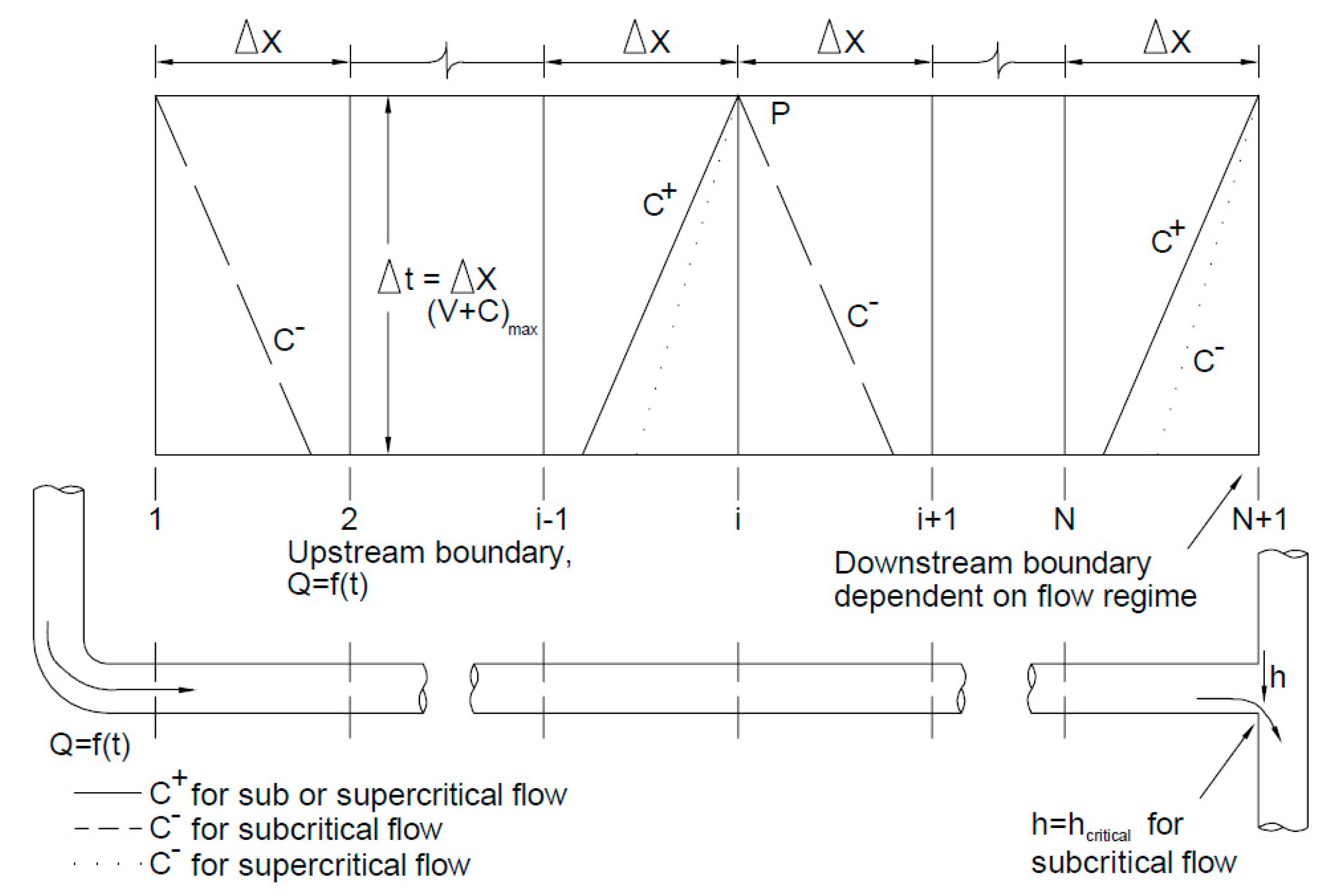
The method of characteristics technique incorporated into DRAINET is appropriate for the simulation of free surface flows in partially-filled drainage pipes [3]. Based on the solution of the St. Venant equations for continuity and momentum, first proposed by Lister [16], this modelling technique represents the fundamental equations as two first order finite difference equations, known respectively as C+ and C− characteristic slopes in the method of a characteristics grid, linking known conditions at time t to conditions at P at one time step in the future.
With reference to Figure 3 it can be shown that,
provided that the calculation time step conforms to the Courant criterion, defined as
where, the wave propagation speed c is defined as c = (gA/T)0.5, S and So are the friction and pipe slopes, respectively, and A and T are the flow cross sectional area and the surface width, respectively. The form of Equation (9) requires a small base flow in the pipe in order that the calculations can commence.
From Figure 3 it can also be seen that only one characteristic is available at system entry or exit. Thus, it is necessary to define boundary equations that may be solved with the appropriate C+ and C− characteristic at these nodes. Previous research in this area has yielded boundary equations for many conditions [3,4,5,6,17,18] including the following:
- Toilet discharge
- Pipe junctions
- Displaced upstream hydraulic jumps
- Flow at the base of a vertical stack
- Solid transport
Figure 3 shows the grid used to represent the progress of a calculation in the method of the characteristics scheme of the type most relevant to the partially filled pipe: unsteady flow regimes experienced in building drainage systems. This is a specified grid system in that the nodal distances along the x axis are pre-defined, while the time step may vary depending on the flow conditions and subject to the current criterion outlined above.
The transport of a solid in a near horizontal drainage pipe under steady flow conditions is characterised by a number of significant changes in the flow depth profile, as shown in Figure 3. The water height behind the solid reduces gradually to a point where the water depth is normal for the particular flow regime due to the inflow and the water immediately in front of the solid is below normal water depth and increases downstream. This bow wave is due to the effects of water tumbling over the solid at a higher-than-normal velocity.
3. Results and Discussion
3.1. Model Comparisons
The characteristics of the solid were selected based on previous work carried out by Swaffield, Gormley, and Campbell [3,4,5] and Gormley et al. [6] where studies were conducted to assess the transport of a range of different solids from 0.85–1.2 specific gravity, with diameters between 25 and 38 mm. The details of the solid characteristics used in the study are presented in Table 1.
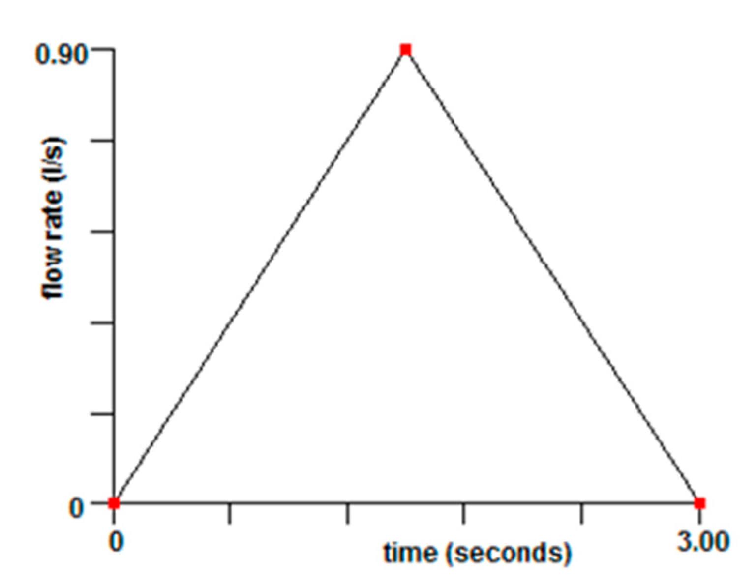
These solids were selected as representative of a range of waste material entering the pipe network and represent a worst-case scenario since in practice faecal stools can disintegrate with time and agitation. These solids were modelled in DRAINET using a representative flush of 1.4 litres as shown below in Figure 4. The Q/T data represents the surge wave from a pour flush device. When applied to the DRAINET 1D method of characteristics, a finite difference model can be used to assess solid transport within the pipe network. DRIAINET effectively solves the St. Venant equations, which handles wave attenuation and applies a relative velocity to solids.
The same scenario was modelled using SPH Dualphysics. The geometry, showing the arrangement of the water inlet is indicated in Figure 5.
In the SPH model, solids are defined as a collection of particles that are given physical properties such as density, mass, and physical dimensions of length and diameter. The intricacies and issues surrounding the definition of these properties will be discussed in the Results/Discussion Section, however, it will be noted here that nuances with fluctuating density throughout the calculation process mean that a fixed definition of a moving object in SPH is very challenging.
SPH Geometry
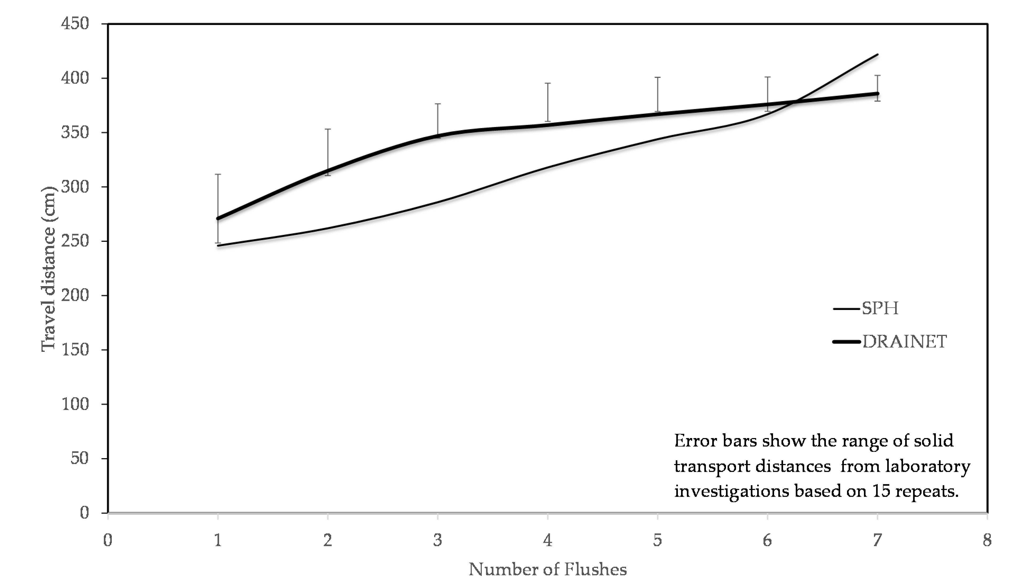
The results of both models are compared in Figure 6 for a solid of specific gravity (SG) 0.85 and in Figure 7 for a solid of SG of 1.1. For these test runs, SPH was set to its default settings.
It can clearly be seen that there is a good correlation between the laboratory results and the results from DRAINET, thus confirming the accuracy of the 1D DRAINET model. The default setting in SPH underestimates solid travel distances, although it overshoots the travel distance in the case of the heavier solid (SG = 1.1).
3.2. Model Calibration
To attempt to align the results more closely with the laboratory investigation results and the DRAINET results, a calibration exercise was carried out to assess the impact of some of the parameters in the SPH model. Modifications were made to the ViscoBoundFactor, solid mass, and density. The effect of modifying these parameters were determined in terms of the solid transportation and flow velocity.
3.2.1. ViscoBoundFactor
ViscoBoundFactor (VBF) influences the artificial viscosity simulated in the model. This can account for friction and pipe roughness that is otherwise not specified, where this parameter influences the interaction between fluid and boundary particles. Gormley and Campbell identified the interaction between the fluid and solid friction as a governing solid transportation principle [4,5] and Princeton determined friction as dependent on fluid viscosity.
A previous study carried out by Barreiro et al. determined the effect of this factor on the velocity of flow by carrying out the experiment for VBFs from 1 to 8, and this was similarly tested in this study. The effect of the VBF on flow velocity was assessed for a similar range of VBF (1–20) by determining the average velocity of the flow in the initial section of pipe for each VBF. Taking the velocity from this initial section ensures no influence on the flow from the vertical drop.
These results were compared with the flow velocity measured in DRAINET to obtain the VBF with the most appropriate flow. Further to this, the solid transportation of each of the VBFs was established. This followed the same procedure for testing the model where the solid transportation was determined for each of test flushes.
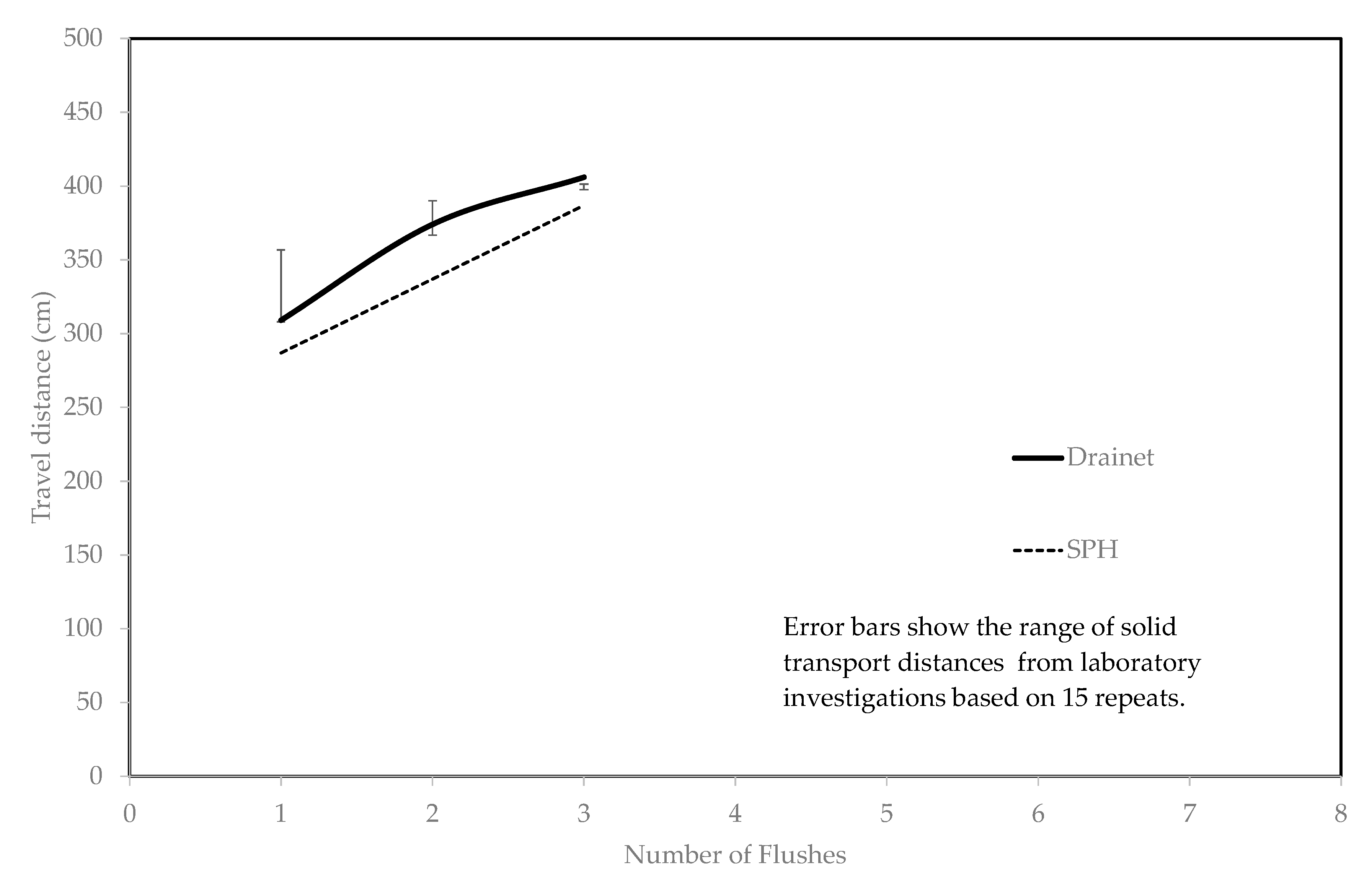
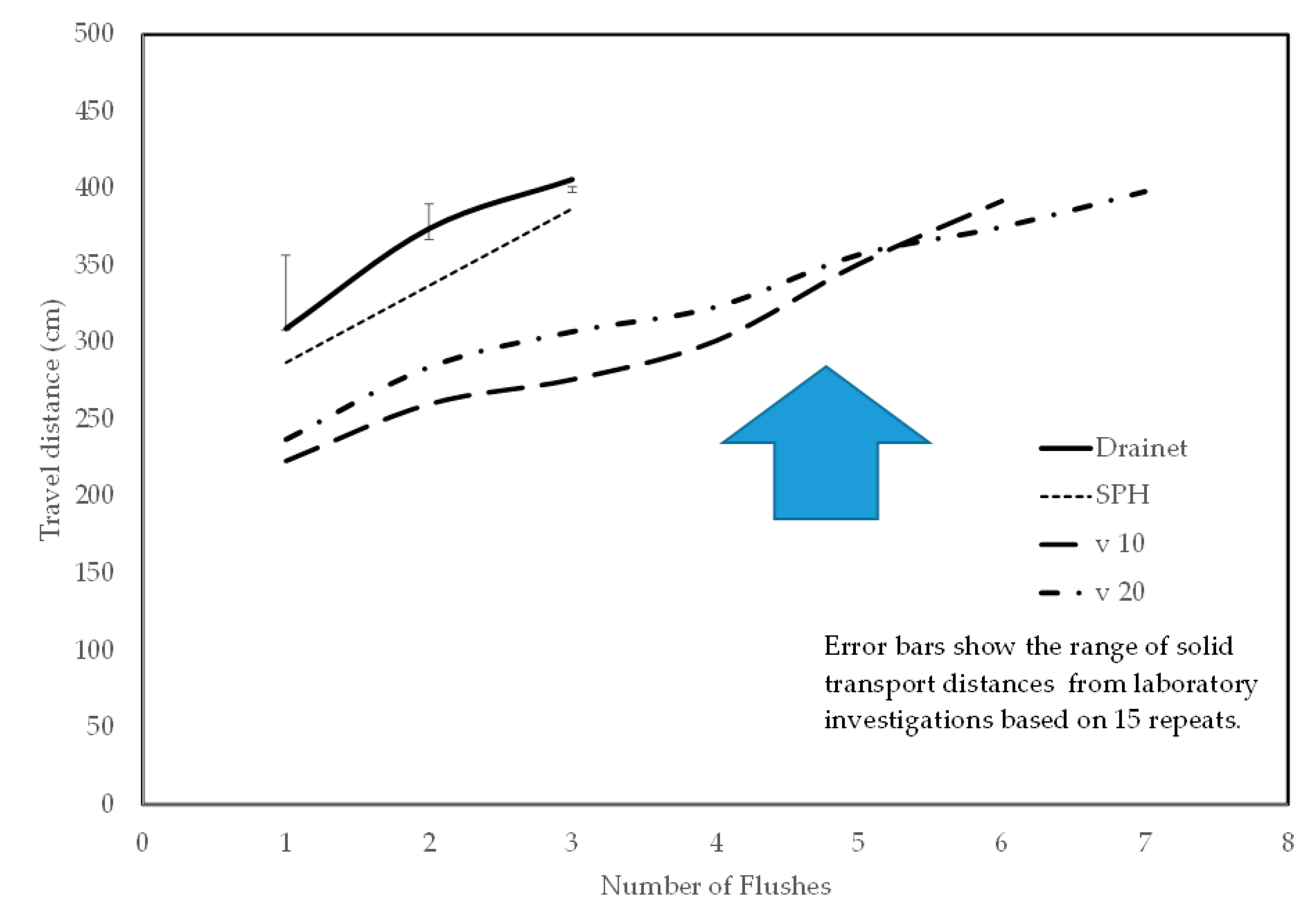
Solid transport was assessed for each of the thre different ViscoBoundFactors (VBFs) (1, 10, and 20) and the ratio of average distance travelled per flush to the average distance travelled in DRAINET was plotted in Figure 8. It can be seen that only the VBF of 1 comes close to the actual physical data obtained from the lab, while DRAINET accurately falls within the range of the laboratory results obtained. For the vcase where the specific gravity is greater than 1 (Figure 9) again, a ViscoBoundFactor of 1 is closest, however, still not as accurate as the DRAINET results.
The discrepancies between the SPH and the DRAINET/laboratory results are not insignificant for both of the cases. While there is a distinct difference between results when different ViscoBoundFactors are used, the closest correlation relates to a ViscoBoundFactor of 1, and attempts to modify the artificial viscosity generally made the correlation worse.
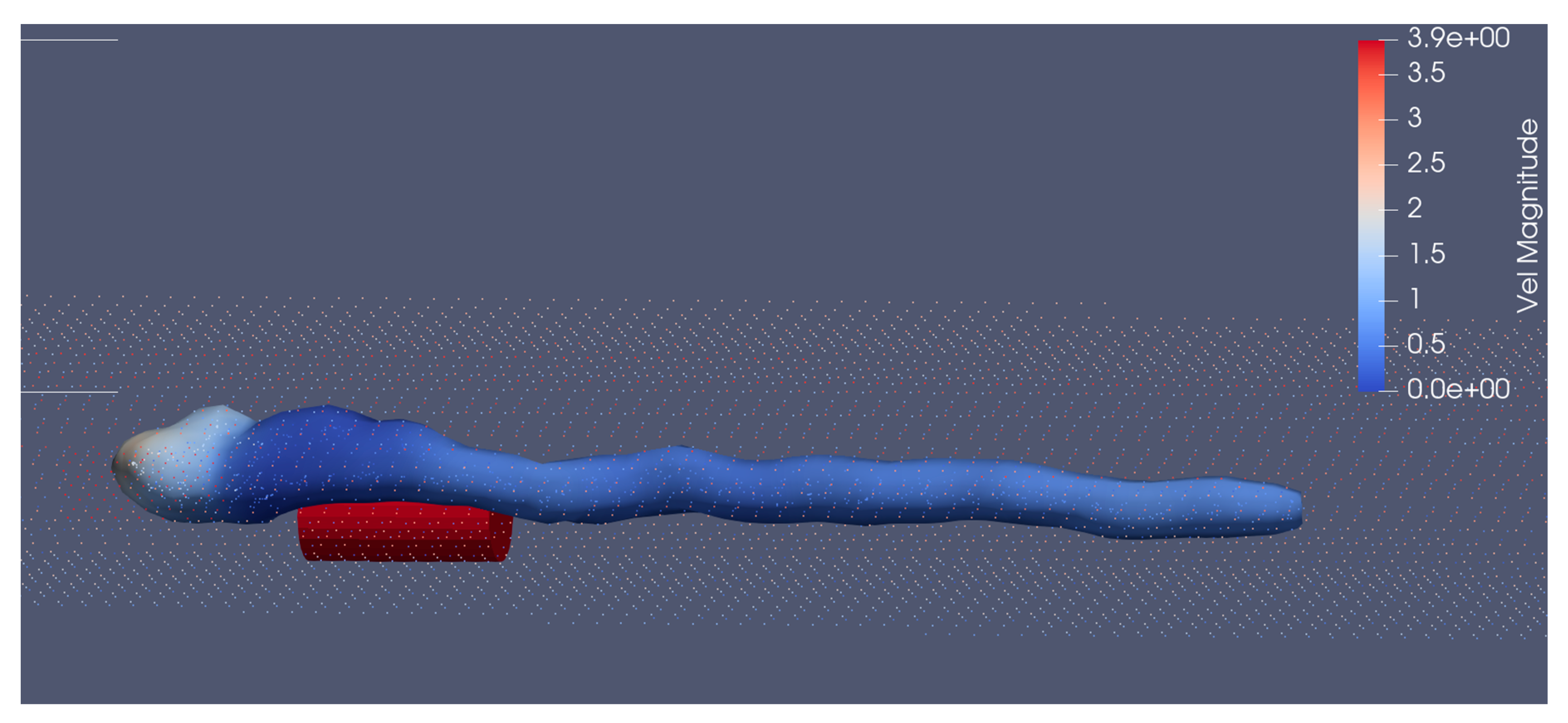
A closer look at the simulation output in Figure 10 show that there is a tendency for the water to tumble over the solid in SPH. It is worth noting that this phenomenon is observed in the laboratory, however, it seems to be exaggerated in SPH. More work is required to investigate the reason for this.
3.2.2. Density and Mass
Within SPH, the mass of particles remains constant throughout a simulation, however, in reality the density fluctuates. Depending on whether the mass or density of the solid is input to the Case_Def.xml file, this could impact the movement of the solid due to this fluctuation in density. Therefore, the difference in solid transportation was assessed between the two for each specific gravity of solids, where the density and mass values are given in Table 1. The challenge comes in defining a solid object in a system where density can fluctuate. Density, specific gravity, and mass are important paraments in relation to solid transport in this context and therefore it was considered necessary to evaluate the definition of the solid by both mass and density.
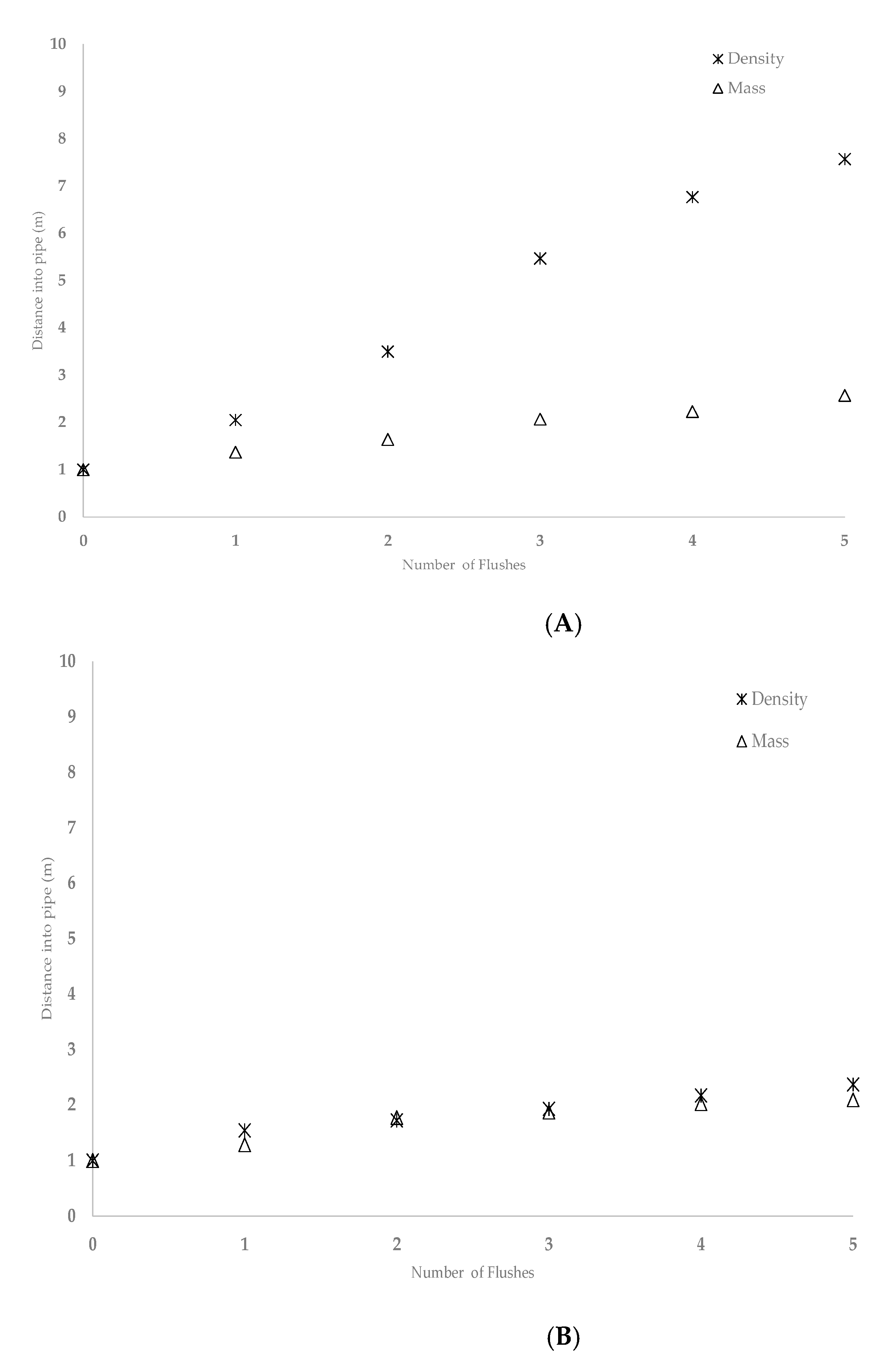
To determine the intensity of the fluctuation in density on the solid transportation, the results having input density and mass to the simulation were recorded. The results from SPH are presented for two different solids over a number of flushes to assess divergence, as shown in Figure 11A,B. The data presented in Figure 11 relate to a ViscoBoundFactor (VBF) of 20.
Where the delta-SPH factor is incorporated into the continuity equation, Equation (6), as a means of reducing the fluctuation of density occurring in Lagrangian particle-based simulations, the results presented in Figure 10 show the effect that inputting the solid density as opposed to solid mass has, particularly on the lighter solid as shown in Figure 11A. For both SGs the transportation distance is greater when the density has been input, where this is likely due to the density fluctuation.
Referring to a solid of 0.85 specific gravity as shown in Figure 11A, after five flushes, the solid movement is significantly greater. As the solid is already less dense than water it will float in the water (whilst considering the limited effect of buoyancy due to the low water usage). As the density fluctuates, this will remain below the water density, and therefore will still be influenced by the buoyancy. In addition to buoyancy, the solid is impacted by external forces, including viscous drag. As the solid is lighter, it is further affected by the force from the fluid, where this instantly increases its distance in comparison to a heavier solid, whilst the impact of density on buoyancy and viscous drag will further increase the solid transportation compared with inputting the solid mass. Furthermore, as lighter solids have a more random nature, this is an additional reason for the difference in results between density and mass.
The difference between mass and density results for a solid with a specific gravity of 1.1 is less noticeable, where this is likely influenced by the solid having a greater density than water and is therefore less impacted by buoyancy. This reduced impact from buoyancy reduces the variation in results between mass and density, whilst the density inclusion in the viscous drag equation accounts for a portion of the fluctuation. The more consistent nature of heavier solids, in comparison to that of the lighter solids, lead to the less scattered results in Figure 11B for SG = 1.1.
4. Conclusions
The benefits of a 3D model to establish efficiency of flushing mechanisms presents a method for the evaluation of physical design geometry in terms of a measurable performance indicator. In this case, the device under investigation was an ultra-low water usage pour flush squat plate toilet as used in developing countries. The system within which this is designed to function is a low-cost simplified sewerage system. Due to the low water usage of the system, the efficiency of the toilet at removing waste is imperative.
The system chosen to model the operation of the device was the DualPhysics solid particle hydrodynamics (SPH), an open source code capable of modelling particles in a flow regime. The parameter used to determine the overall performance was solid transport distance. The results of the SPH study were compared to a fully validated finite difference model (DRAINET) and laboratory investigations to replicate the low water usage devices in question. A standard cylindrical solid was used to establish performance.
While SPH offers a simple platform from which to setup an investigation, replicating the movement of a cylindrical solid in a turbulent flush proved particularly difficult. Issues with defining viscosity and defining density/mass of the solid were particularly challenging within the code. Additionally, the computational cost of SPH is very high with little overall benefit in a larger complex system. It is often the case that modelling moving solid objects in free surface turbulent flows causes problems with stability, accuracy, and error in computation, however, the combination of these elements within this application was particularly problematic as evidenced by the divergence of the solid transport results between the laboratory investigation, DRAINET 1D, and SPH modelling. Further work to refine interpolation methodologies, improve accuracy, and limit error is required for this application.
Overall, SPH was found to be useful for characterising the geometry of the pour flush pan but not for whole system assessment. A hybrid method is thus recommended whereby the design and performance characteristics for the input stage can be modelled in SPH but the whole system pipe network evaluation is better suited to the 1D DRAINET model.
Author Contributions
Conceptualization, M.G.; methodology, M.G. and S.M.; software, M.G. and S.M.; validation, M.G.; formal analysis, M.G. and S.M.; resources, M.G.; data curation, M.G. and S.M.; writing—original draft preparation, S.M. and M.G.; writing—review and editing, M.G. and S.M.; supervision, M.G.; project administration, M.G. All authors have read and agreed to the published version of the manuscript.
Funding
This research received no external funding.
Institutional Review Board Statement
Not applicable.
Informed Consent Statement
Not applicable.
Data Availability Statement
Data is contained within the article.
Acknowledgments
We acknowledge the support of The Institute for Sustainable Building design, Architectural Engineering discipline, for assistance with this research.
Conflicts of Interest
The authors have no conflict of interest to declare.
References
- Gormley, M.; Williams, L.A.; Ongole, B. Up-scaling sanitation provision using mixed design methodologies and failure risk assessment: A case study of Marikuppam, India. J. Water Sanit. Hyg. Dev. 2018, 8. [Google Scholar] [CrossRef] [Green Version]
- Jean, N.J.; Gormley, M. Modelling water trap seal boundary conditions in building drainage systems: Computational fluid dynamics analysis of unsteady friction to improve accuracy. Build. Serv. Eng. Res. Technol. 2017, 38, 580–601. [Google Scholar] [CrossRef]
- Swaffield, J.; Gormley, M.; Wright, G.; McDougall, I. Transient Free Surface Flows in Building Drainage Systems; Routledge: Abingdon, UK, 2015. [Google Scholar] [CrossRef]
- Gormley, M.; Campbell, D.P. The transport of discrete solids in above ground near horizontal drainage pipes: A wave speed dependent model. Build. Environ. 2006, 41. [Google Scholar] [CrossRef]
- Campbell, D.P.; Gormley, M. Modelling water reduction effects: Method and implications for horizontal drainage. Build. Res. Inf. 2006, 34, 131–144. [Google Scholar] [CrossRef]
- Gormley, M.; Mara, D.D.; Jean, N.; McDougall, I. Pro-poor sewerage: Solids modelling for design optimisation. Proc. Inst. Civ. Eng. Munic. Eng. 2013, 166. [Google Scholar] [CrossRef]
- Gormley, M.; Kelly, D.A. Pressure transient suppression in drainage systems of tall buildings. Build. Res. Inf. 2018. [Google Scholar] [CrossRef]
- Crespo, A.J.C.; Dominguez, J.M.; Gesteira, M.G.; Barreiro, A.; Rogers, B.D.; Longshaw, S.; Canelas, R.; Vacondio, R. User Guide for DualSPHysics Code v3.0; University of Vigo: Vigo, Spain; The University of Manchester: Manchester, UK; Johns Hopkins University: Baltimore, MA, USA, 2013; pp. 1–59. [Google Scholar]
- Monaghan, J.J. Smoothed Particle Hydrodynamics. Annu. Rev. Astron. Astrophys. 1992, 30, 543–574. [Google Scholar] [CrossRef]
- Monaghan, J.J. Smoothed particle hydrodynamics. Rep. Prog. Phys. 2005, 68, 1703–1759. [Google Scholar] [CrossRef]
- Sivanesapillai, R.; Falkner, N.; Hartmaier, A.; Steeb, H. A CSF-SPH method for simulating drainage and imbibition at pore-scale resolution while tracking interfacial areas. Adv. Water Resour. 2016, 95, 212–234. [Google Scholar] [CrossRef]
- Springel, V.; Dullemond, C. Smoothed Particle Hydrodynamics; Heidelberg University: Heidelberg, Germany, 2014. [Google Scholar]
- Verbrugghe, T.; Stratigaki, V.; Altomare, C.; Domínguez, J.; Troch, P.; Kortenhaus, A. Implementation of Open Boundaries within a Two-Way Coupled SPH Model to Simulate Nonlinear Wave–Structure Interactions. Energies 2019, 12, 697. [Google Scholar] [CrossRef] [Green Version]
- Gormley, M. Air pressure transient generation as a result of falling solids in building drainage stacks: Definition, mechanisms and modelling. Build. Serv. Eng. Res. Technol. 2007, 28. [Google Scholar] [CrossRef]
- Barreiro, A.; Domínguez, J.M.; CCrespo, A.J.; González-Jorge, H.; Roca, D.; Gómez-Gesteira, M. Integration of UAV photogrammetry and SPH modelling of fluids to study runoff on real terrains. PLoS ONE 2014, 9, e111031. [Google Scholar] [CrossRef] [Green Version]
- Crespo, A.J.C.; Domínguez, J.M.; Rogers, B.D.; Gómez-Gesteira, M.; Longshaw, S.; Canelas, R.; Vacondio, R.; Barreiro, A.; García- Feal, O. DualSPHysics: Open-source parallel CFD solver based on Smoothed Particle Hydrodynamics (SPH). Comput. Phys. Commun. 2015, 187, 204–216. [Google Scholar] [CrossRef]
- Lister, M. The Numerical Solution of Hyperbolic Partial Differential Equations by the Method of Characteristics. Math. Methods Digit. Comput. 1960, 1, 165–179. [Google Scholar]
- Swaffield, J. Transient Airflow in Building Drainage Systems; Routledge: London, UK, 2010. [Google Scholar]
Figure 1.
Dimensioned elevation, and isometric, of the system under consideration in this study.

Figure 2.
Flow velocity and ViscoBoundFactor (VBF) [8].
Figure 2.
Flow velocity and ViscoBoundFactor (VBF) [8].

Figure 3.
Application of the method of a characteristics-specified time interval grid for a partially filled pipe flow with known entry and exit boundary equations.
Figure 3.
Application of the method of a characteristics-specified time interval grid for a partially filled pipe flow with known entry and exit boundary equations.

Figure 4.
Flowrate against time graph for pour flush.

Figure 5.
Smoothed particle hydrodynamics (SPH) geometry and the arrangement of the water inlet and solid positioning.
Figure 5.
Smoothed particle hydrodynamics (SPH) geometry and the arrangement of the water inlet and solid positioning.

Figure 6.
Comparison between laboratory results, DRAINET results, and SPH results for a simulated solid of 80 mm length with a diameter of 36 mm, a specific gravity (SG) of 1.1, a mass of 85 g, and a density of 1100 kgm−3.
Figure 6.
Comparison between laboratory results, DRAINET results, and SPH results for a simulated solid of 80 mm length with a diameter of 36 mm, a specific gravity (SG) of 1.1, a mass of 85 g, and a density of 1100 kgm−3.

Figure 7.
Comparison between laboratory results, DRAINET results, and SPH results for a simulated solid of 80 mm length with a diameter of 36 mm, a specific gravity (SG) of 0.85, a mass of 69 g, and a density of 850 kgm−3.
Figure 7.
Comparison between laboratory results, DRAINET results, and SPH results for a simulated solid of 80 mm length with a diameter of 36 mm, a specific gravity (SG) of 0.85, a mass of 69 g, and a density of 850 kgm−3.

Figure 8.
Effect on solid transport of changing the ViscoBoundFactor. Results for three values—1 (SPH), 10 (VBF10), and 20 (VBF20) shown in comparison to DRAINET and results from laboratory investigations for the case where the specific gravity was 0.85.
Figure 8.
Effect on solid transport of changing the ViscoBoundFactor. Results for three values—1 (SPH), 10 (VBF10), and 20 (VBF20) shown in comparison to DRAINET and results from laboratory investigations for the case where the specific gravity was 0.85.

Figure 9.
Effect on solid transport of changing the ViscoBoundFactor. Results shown in comparison to DRAINET and results from laboratory investigations for the case where the specific gravity was 1.1.
Figure 9.
Effect on solid transport of changing the ViscoBoundFactor. Results shown in comparison to DRAINET and results from laboratory investigations for the case where the specific gravity was 1.1.

Figure 10.
Image of the flow velocity profile over the solid in SPH.

Figure 11.
The effect of density on solid transportation. SG = 0.85 (A) and SG = 1.1 (B).


Table 1.
Solid characteristics.
| Length | 80 mm | 80 mm |
|---|---|---|
| Diameter | 36 mm | 36 |
| Specific Gravity | 0.85 | 1.1 |
| Mass | 69 g | 85 g |
| Density | 850 (kg/m3) | 1100 (kg/m3) |
| Material | PVC | PVC |
Publisher’s Note: MDPI stays neutral with regard to jurisdictional claims in published maps and institutional affiliations. |
© 2021 by the authors. Licensee MDPI, Basel, Switzerland. This article is an open access article distributed under the terms and conditions of the Creative Commons Attribution (CC BY) license (http://creativecommons.org/licenses/by/4.0/).
Share and Cite
MDPI and ACS Style
Gormley, M.; MacLeod, S. Towards a Solid Particle Hydrodynamic (SPH)-Based Solids Transport Model Applied to Ultra-Low Water Usage Sanitation in Developing Countries. Water 2021, 13, 441. https://doi.org/10.3390/w13040441
AMA Style
Gormley M, MacLeod S. Towards a Solid Particle Hydrodynamic (SPH)-Based Solids Transport Model Applied to Ultra-Low Water Usage Sanitation in Developing Countries. Water. 2021; 13(4):441. https://doi.org/10.3390/w13040441
Chicago/Turabian StyleGormley, Michael, and Sophie MacLeod. 2021. "Towards a Solid Particle Hydrodynamic (SPH)-Based Solids Transport Model Applied to Ultra-Low Water Usage Sanitation in Developing Countries" Water 13, no. 4: 441. https://doi.org/10.3390/w13040441
Note that from the first issue of 2016, this journal uses article numbers instead of page numbers. See further details here.