
Gross Solids Content Prediction in Urban WWTPs Using SVM
by
 , ,
, ,
Vanesa Mateo Pérez
 ,
,
José Manuel Mesa Fernández
*,
Francisco Ortega Fernández
and
Joaquín Villanueva Balsera
Project Engineering Area, University of Oviedo, Independencia, n° 13, 33012 Oviedo, Spain
*
Author to whom correspondence should be addressed.
Water 2021, 13(4), 442; https://doi.org/10.3390/w13040442
Submission received: 20 December 2020
/
Revised: 26 January 2021
/
Accepted: 5 February 2021
/
Published: 8 February 2021
(This article belongs to the Section Wastewater Treatment and Reuse)
Abstract
:The preliminary treatment of wastewater at wastewater treatment plants (WWTPs) is of great importance for the performance and durability of these plants. One fraction that is removed at this initial stage is commonly called gross solids and can cause various operational, downstream performance, or maintenance problems. To avoid this, data from more than two operation years of the Villapérez Wastewater Treatment Plant, located in the northeast of the city of Oviedo (Asturias, Spain), were collected and used to develop a model that predicts the gross solids content that reaches the plant. The support vector machine (SVM) method was used for modelling. The achieved model precision ( = 0.7 and MSE = 0.43) allows early detection of trend changes in the arrival of gross solids and will improve plant operations by avoiding blockages and overflows. The results obtained indicate that it is possible to predict trend changes in gross solids content as a function of the selected input variables. This will prevent the plant from suffering possible operational problems or discharges of untreated wastewater as actions could be taken, such as starting up more pretreatment lines or emptying the containers.
1. Introduction
Municipal wastewater is derived from domestic, commercial, and industrial waste streams, along with storm water runoff. In addition to fecal matter, sewage contains a variety of suspended and floating debris, including sand and other entrained inert solids, paper, plastics, rags, and other debris. The presence of gross solids in the collectors can help to create several problems [1,2]. In the sections of the sewer network in which the water circulates by gravity, the solids combine with the fats and generate blockages. When water is circulated by pumping, the presence of gross solids can cause pump jams and pump well overflows with resulting contamination problems.
As wastewater enters a treatment facility, it typically flows through a step called preliminary treatment. This stage, which removes gross solids and coarse suspended and floating matter, has not received much research attention, and it is highly dependent on the initial design characteristics of the plant [3,4,5]. However, its impact on the management, operation, and maintenance of one of these wastewater treatment plants (WWTPs), as well as its influence on the performance of the subsequent treatment stages, is very important. In this pretreatment stage, various operations are carried out, such as roughing, sand removal, and degreasing. Generally, a screen removes large floating objects, such as rags, cans, bottles, and sticks, that may clog pumps, small pipes, and downstream processes. If gross solids are not removed, they become entrained in pipes and other moving parts of the treatment plant and can cause substantial damage and inefficiency in the process [6,7]. Screens are generally placed in a chamber or channel and inclined towards the flow of the wastewater. The inclined screen allows debris to be caught on the upstream surface of the screen, but it also allows access for manual or mechanical cleaning.
The operational management of this initial stage usually faces various problems, such as the following:
- Gross solids on days without rain are deposited in the bottom of the collectors, and when there is heavy rain, they are suddenly drawn into the treatment plant [8]. Numerous researchers have studied the consequences of these solids in sewage systems [9,10,11,12,13,14]. The arrival of all these gross solids at the WWTP can cause blockages in the equipment and, consequently, lead to discharge of untreated wastewater into rivers. Knowing of the arrival of solids as soon as possible would allow for anticipating and putting more pretreatment lines into service, avoiding those blockages.
- Another operational problem to be faced is the need to have enough containers for the gross solids and to avoid having to pile them on the ground in a precarious way. By predicting the arrival of gross solids earlier, it is possible to ensure the availability of empty containers.
The improvement of operations in treatment plants and its impact on their performance, the reduction of energy consumption, and the reduction of maintenance costs is receiving more and more attention from researchers [15,16,17,18]. The increasingly strict legal and environmental requirements force us to seek an improvement in the operation of these facilities [19,20]. An important way of optimizing this operation is the development of mathematical process models. Many authors have developed mathematical models of the different treatment stages of wastewater treatment plants [21,22]. Although the preliminary treatment stage has been less studied, in part due to its great dependence on the initial plant design, its impact on the performance of later stages is unquestionable.
Moreover, the treatment processes of sewage treatment plants are monitored continuously, but often the data collected are not sufficiently exploited [23]. Therefore, the use of the available data to improve management from the first treatment processes in the WWTP will result in an improvement in the performance of the later stages, a decrease in energy consumption, fewer installation maintenance problems, and, finally, in a better quality of the outlet water.
Therefore, the main objective of this work is to predict the gross solids content in wastewater to improve the operation of treatment plants. Having this new model will help the operators of the WWTPs make the most appropriate decisions, reducing the possibility of the problems described above. No reference to similar works (developing a prediction model for this operational parameter) was found in the literature review carried out by the authors, which indicates the novelty of this study.
This paper is divided into three main sections. Section 2 describes the characteristics of the WWTP under study, the acquisition and processing of data, and the mathematical techniques used in the development of the model. Next, in Section 3, the results obtained are presented and discussed, both in the model training process and in its validation. Finally, the main contributions of the study are highlighted in Section 4.
2. Materials and Methods
2.1. Case Study
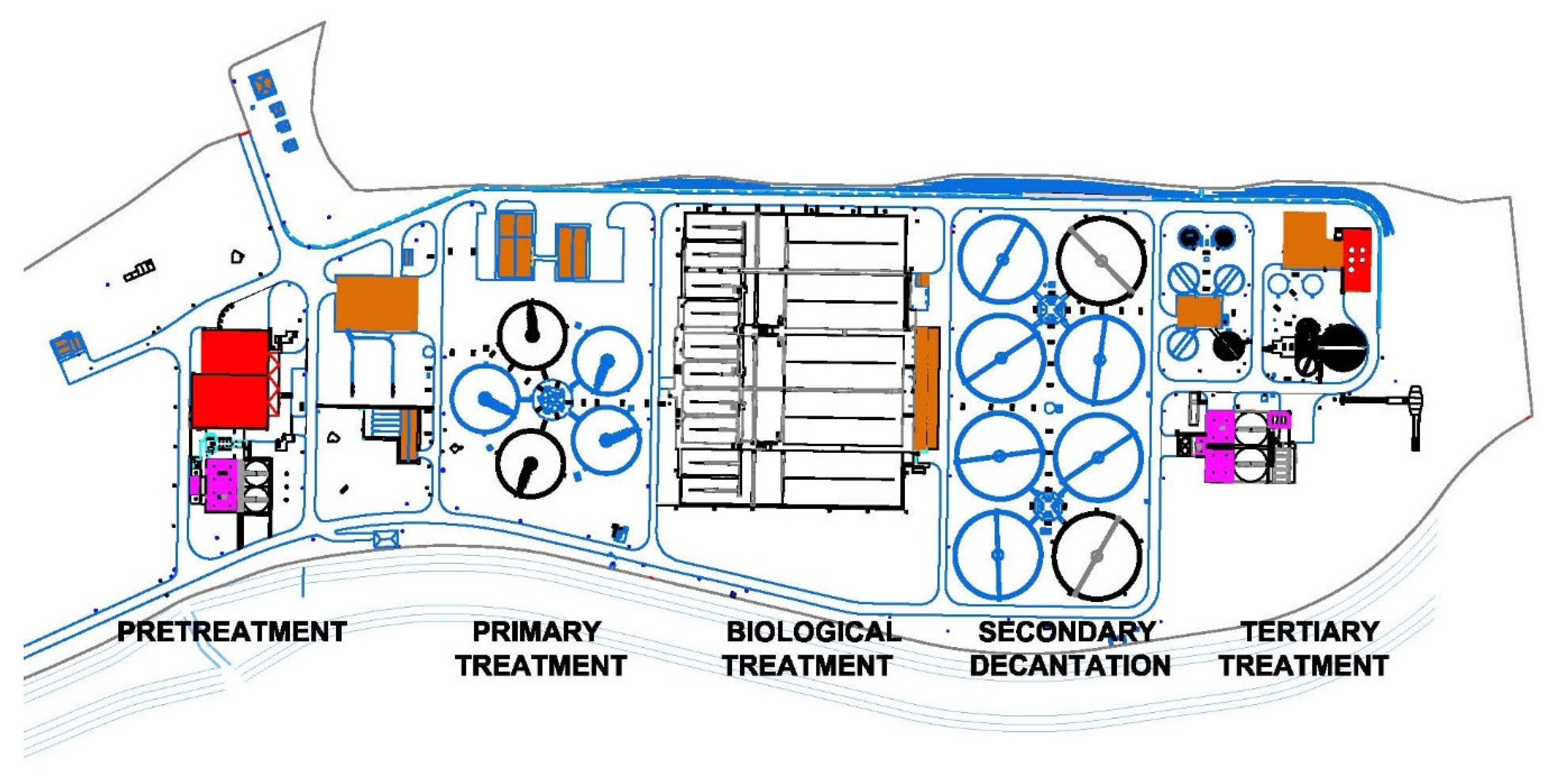
The Villapérez Wastewater Treatment Plant is located in the northeast of the city of Oviedo (Asturias, Spain) and occupies an area of nearly 21 hectares (Figure 1). It provides service to an approximate population of 723,000 equivalent inhabitants. The wastewater to Villapérez arrives through a unitary network of collectors that has an approximate length of 75 km. This network includes 44 spillways. Collector diameters range from 600 to 2000 mm with sections in gravity and in impulsion.
As can be seen in Figure 2, the wastewater treatment in Villapérez WWTP begins with a pretreatment stage in which the larger solids, sands, and fats are removed. Subsequently, the water is taken to primary settling by gravity. The water then goes to biological treatment where organic matter, nitrogen, and phosphorus are removed. This treatment involves the passage of water through several anoxic chambers, anaerobic and aerobic. The next stage is secondary settling, which is carried out via gravity. Finally, the tertiary treatment stage consists of a physical–chemical treatment, lamellar settling, and filtration.
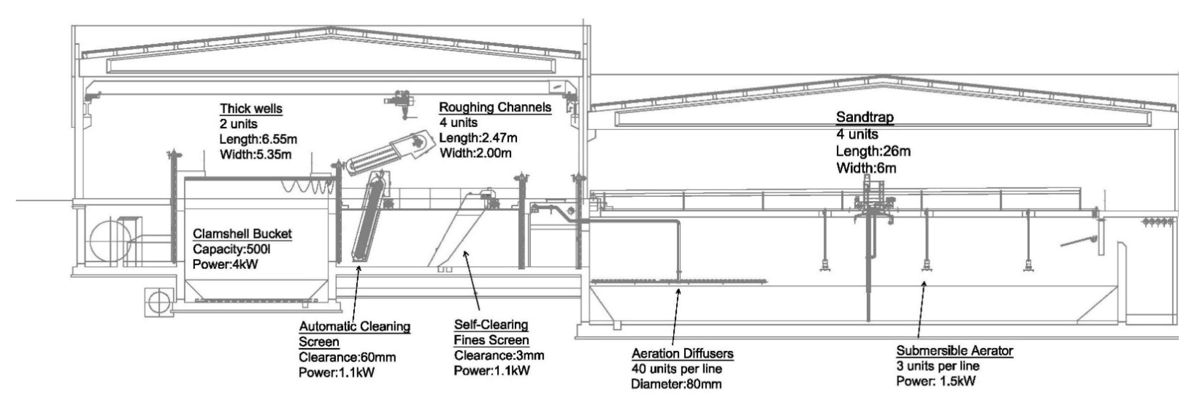
The pretreatment section has the capacity to treat an inflow of 8.5 m3/s (734,400 m3/day) and starts with two thick wells, equipped with a 500-L clamshell bucket (Figure 2). The plant then has four roughing channels, each of which includes an automatic cleaning screen with a 60 mm clearance and a self-cleaning fines screen with a 3 mm clearance and an inclination of 50°.
In order to size the installation, Table 1 shows the main design parameters of the installation, including the legally established [24] values for the discharge of treated water.
The Villapérez treatment plant receives around 19 tons of roughing solids monthly. As already indicated, although these roughing solids are produced continuously, they are stored at the bottom of the collectors and suddenly arrive at the treatment plant when heavy rains occur. In episodes of intense rains, the arrival of up to 4 tons of solids in one hour has been recorded.
2.2. Data
All data used in this work were collected in the period from 1 March 2017 to 24 June 2019 and come from different sources, as follows:
- Data related to wastewater were obtained through the SCADA software (Supervisory Control and Data Acquisition) of the WWTP. This system registers 226 parameters every 9 minutes from measuring equipment and sensors distributed all over the treatment plant. From this set of data, the data set associated to the measurement of input parameters in the raw water during the pretreatment stage was used. The parameters measured in the raw water are the input flow rate, pH, raw water temperature, conductivity, and ammonia. Data associated with these variables were identified by date and time of the data measurement.
- Gross solids data were collected from the container removal delivery notes (provided by the waste management entity), which contain the actual information of the waste total weight inside each container. The number of containers in the study period was 165. Their filling times were used as time intervals to group the data from the SCADA system.
- Climate data were obtained from the Spanish State Agency for Meteorology website (Agencia Estatal de Meteorología, Aemet) and pluviometry data (instantaneous and accumulated rainfall) were obtained from the plant’s own weather station. All of them were also grouped according to the intervals in which the containers were filled. From these data, a new variable calculated from the instantaneous precipitation was also created, corresponding to the number of previous days without rain.
The obtained data set (165 cases) was divided into two groups. Eighty percent of the data were used for training the support vector machine (SVM) model, and the remaining 20% were kept for validating the model.
Statistical data for the variables initially considered in the study are presented in Table 3. As indicated above, the reference is the time interval (Time) from when an empty container was placed to when it was removed. When each container was removed, it was weighed, and the data were recorded on the corresponding delivery note. The data corresponding to each one of these periods were summarized by calculating for each variable its minimum, mean, and maximum values, as shown in Table 3.
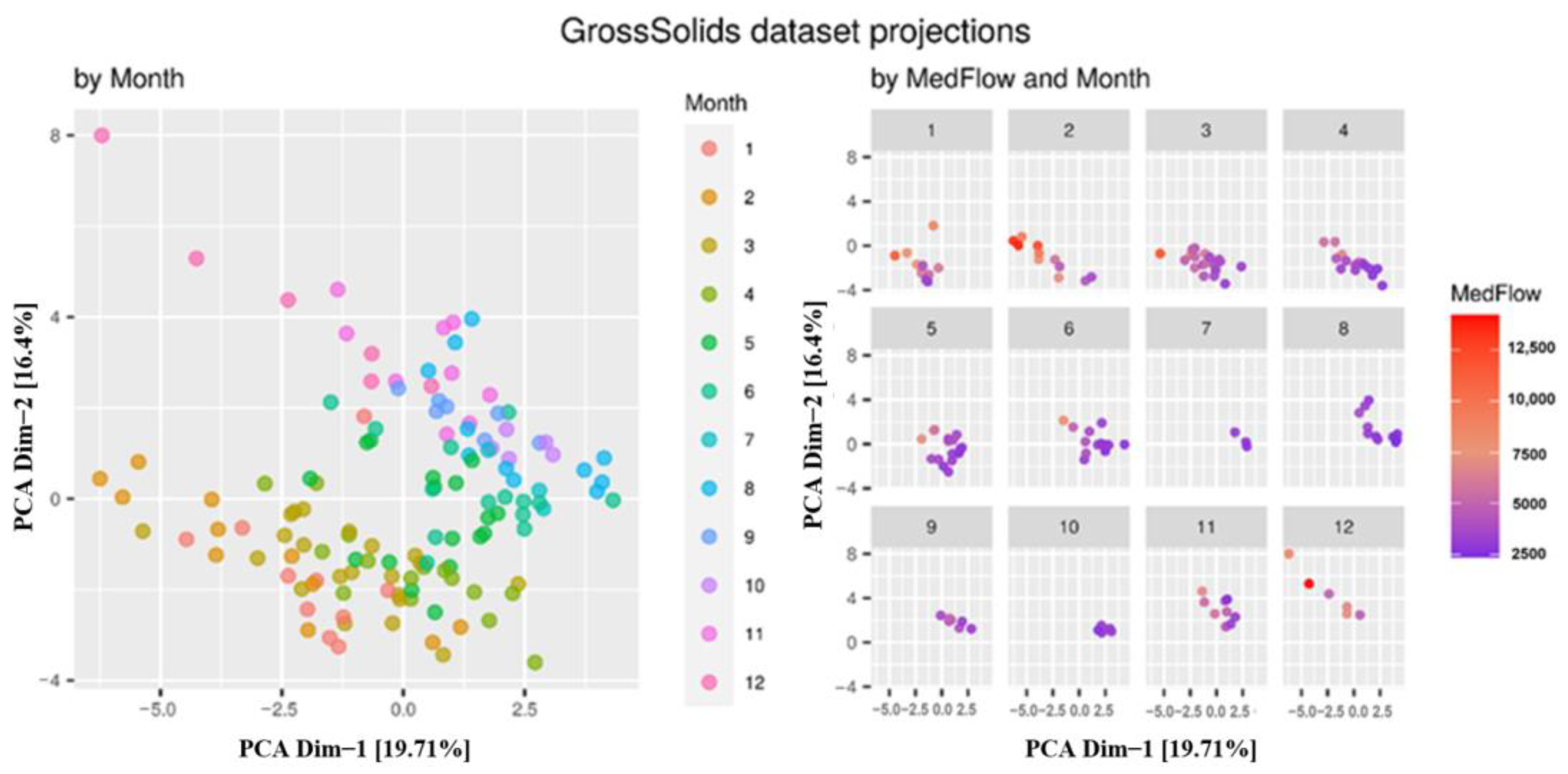
Different statistical analyses were performed to explore the initial data set in order to identify the existence of outliers, as well as to confirm the quality of the data. Among them, we can highlight the principal component analysis (PCA) projection shown in Figure 4. The data were projected in the two main dimensions, which are those that best represent the initial data set in terms of minimum squares. In this figure, on the left, each case of the study is represented with a different color depending on the month of the year in which the sample was taken. In addition, the graph on the right shows the same PCA projection but with the cases separated by month and the average flow (MedFlow) represented with a color scale. These monthly projections clearly reflect that the months with usually higher rainfall present higher inflow into the WWTP, which is a sign of the quality of the training patterns. On the other hand, it is possible to observe in Figure 4 that the cases that are isolated in the complete PCA projection (on the left in the figure), which could initially be considered outliers, correspond to a continuous trend in the cases of Month 12 (December).
2.3. Methods
Different data-based techniques have been used to model different WWTP parameters, such as artificial neural networks (ANNs), fuzzy inference systems (FISs), adaptive neural fuzzy inference systems (ANFISs), and random forest (RF) [15]. In this paper, the method used was support vector machine (SVM), which has been successfully used in many different fields.
SVM refers to a set of supervised learning algorithms developed by Vladimir Vapnik and his team at AT&T laboratories [25]. Although initially developed as a method for binary classification, its application has been extended to multiple classification and regression problems. SVM has been successfully used in many different fields, such as computer vision, character recognition, text and hypertext categorization, classification, natural language processing, and time series analysis [26,27,28]. This is because this method has shown good generalization ability, avoiding the problems of training overfitting that occur in other similar methods [29]. Recently, it has also been used in the field of wastewater treatment to predict different parameters of the treatment process [30,31,32,33,34,35,36,37].
The core of this method is a kernel-based algorithm. Its predictions for new inputs depend on the kernel function evaluation for a subcategory of occurrences during a training stage. The objective of this method is to find a function to minimize the final error in Equation (1):
where y(x) is the predicted value, w is the vector of parameters that define the model, b is the value of the bias, and ϕ(x) fixes the feature space transformation. In this method, the error function that appears in the simple linear regression (Equation (2)) is replaced by an -insensitive error function (Equation (3)). The latter assigns a zero to values when exceeds the difference between the target (tn) and the predicted value (yn). If the difference is not less than , the error function maintains its value.
To minimize Equation (4), a cost (C) is also assigned to the difference between the target and predicted values, where y(x) is the value that Equation (2) predicts, t is the searched target function, ϵ is the margin where the function does not penalize, and C is the penalty. The process is optimized, but the initial function (Equation (2)) increases in complexity (Equation (5)), where α is one solution for the optimization problem that Lagrangian Theory makes possible.
The data are transformed by the function to a higher-dimensional feature space. This increases the accuracy of the nonlinear problem. Thus, the final function resembles Equation (6).
Likewise, as in many other data-based modeling techniques, the quantity and quality of data greatly affect the results obtained. In this case, it is necessary to take into account that the quality of the data collected in these facilities usually presents various reliability problems due to the difficult environmental working conditions of the sensors, which implies a high variation and even errors in the measurements obtained [38]. Therefore, considerable effort was put into collecting data over more than two years from various sources. In this way, the data include information of a seasonal nature, changes in domestic or industrial activity, long periods of intense rains or dry weather, etc. Thus, they are representative of the normal operating conditions at the installation. Subsequently, these data were carefully processed to avoid missing, wrong, or incomplete data to obtain 165 verified patterns to train the model (80%) and to validate the results (20%).
The kernel choice and the particular selection of adjustable kernel parameters have an important influence on the performance of the model [39]. This work was developed by trying various commonly used types of kernel functions, such as linear, polynomial, sigmoid, and radial basis functions [40]. The best kernel for classification in general is the Gaussian radial basis function (RBF) because it produces the highest overall accuracy and highest overall kappa [41].
A grid search methodology with 10-fold cross-validation on the training set was applied to establish the best type of kernel function and to retrieve the optimal values for the model parameters. This k-fold cross-validation procedure is an extensively used approach for assessing the values of model architecture parameters [42,43]. After this process, the RBF was the kernel with the best results (Equation (7)):
where σ is a free parameter and ||x1 − x2|| is the Euclidean distance between points x1 and x2.
R statistical software was selected to program the proposed methodology [44].
3. Results and Discussion
As a result of the training process, an SVM model was obtained that predicts the gross solids in tons based on the variables listed in Table 3.
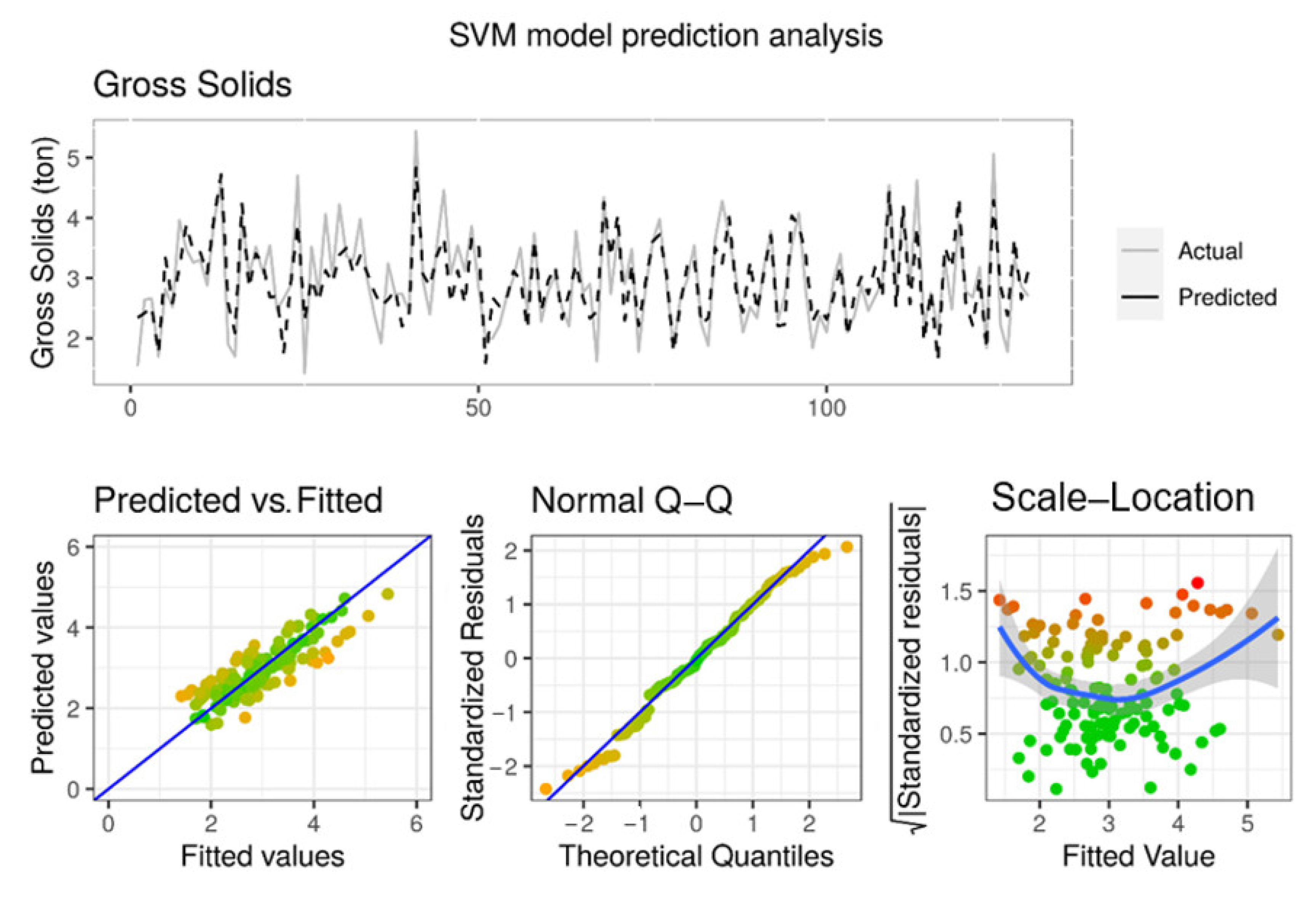
Figure 5 presents different analyses carried out to validate the results of the training process of the SVM model obtained. At the top of the figure, the temporal evolution of the actual values is compared with that predicted from the training data set. It is possible to observe that the model can detect when changes occur in the content of gross solids arriving at the treatment plant.
At the bottom of Figure 5, several graphs are included to represent the error made by the SVM model. The “Prediction vs. Fitted” graph contrasts the actual measured values against the values predicted by the SVM model. It can be seen that all the estimated cases are around the blue line that represents the theoretical behavior of perfect prediction. In the “Normal Q–Q” graph it can be seen that the standardized errors generated by the SVM model in its estimation have a behavior almost identical to the expected theoretical behavior. A greater deviation can be seen at the ends of the line, which is confirmed in the “Scale–Location” graph that shows the estimation error made in each case. In this last graph, it can be seen that those gross solids values lower than 2 tons or higher than 4 tons show an increase in the standardized residuals.
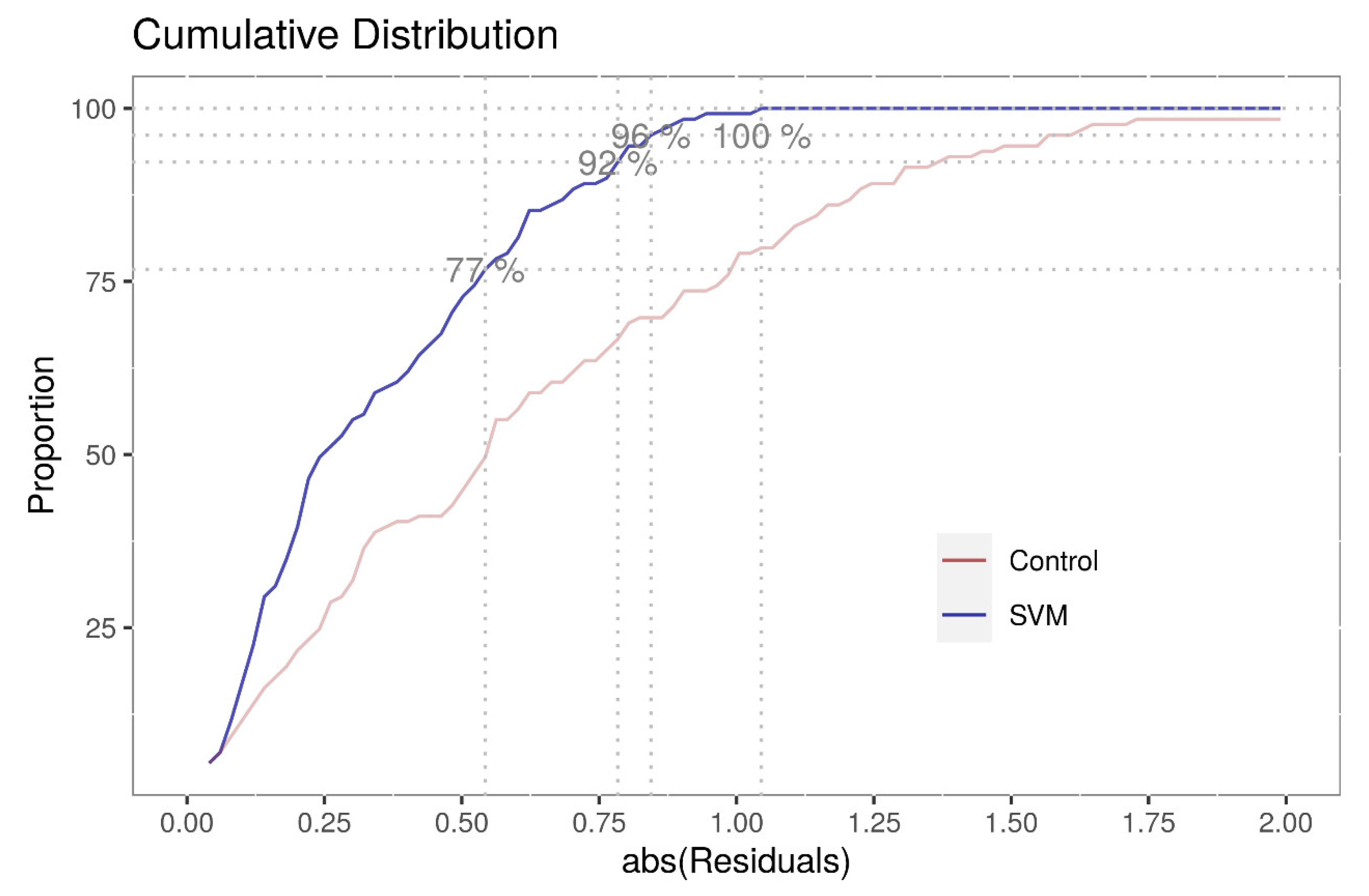
In Figure 6, the curve of the cumulative percentage of successes by the SVM model is represented in blue with increasing tolerance of the estimation error (residuals). The control curve (in red in Figure 6) represents the cumulative success rate achieved by the sewage plant operators, estimated from the mean value of the historical data. A significant improvement can be observed in the results of the SVM model compared to the estimation of the plant control.
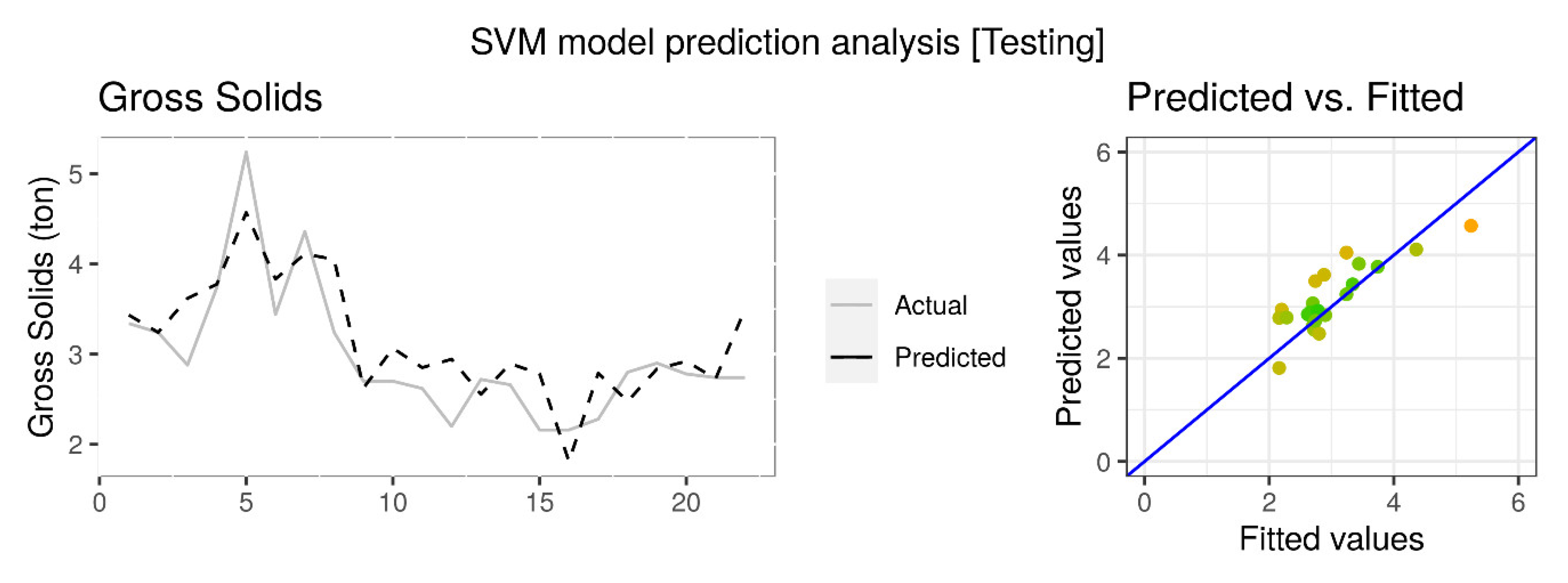
Figure 7 shows the estimated and actual gross solids values over time, corresponding to the validation data set. It is possible to observe that the model can detect when changes occur in the content of gross solids arriving at the treatment plant.
The coefficient of determination is a statistical indicator that compares the accuracy of the model to the accuracy of a trivial benchmark model wherein the prediction is just the mean of all the samples [45]. The performance of the SVM model was measured using the adjusted coefficient of determination () an adjustment for the coefficient of determination that takes into account the number of variables in a data set [46]. It also penalizes you for points that do not fit the model.
Here, n is the number of points in the data sample, k is the number of variables in the model, and R2 is the coefficient of determination.
In this case, although the accuracy of the SVM model obtained was not very high, = 0.7093 for training data and = 0.6869 for validation data, it is enough for predicting trend changes in gross solids recovery during the pretreatment phases. The final model presented mean squared error (MSE) values of 0.426 in training and 0.435 in validation testing. With these results, the resulting final model will provide relevant information to the operators of the WWTP, anticipating problems such as blockages in the equipment or untreated wastewater discharges into the river.
Table 4 includes the most relevant variables for the SVM model when predicting the arrival of gross solids at the WWTP. The two first ones, the week and day of the year, are related to the seasonal component of this variable. An increase in the amount of rain supposes a greater drag on the solids deposited in the collectors, while the pH is an indicator of the amount of flow that reaches the treatment plant from industrial activities. The pH of water from domestic activities is relatively constant, while that from industrial activities alters it, sometimes raising it and sometimes lowering it. One of the consequences is the so-called “weekend effect”. Since the Villapérez WWTP receives a significant portion of wastewater from industrial facilities, the activity of which decreases on weekends and holidays, the resulting reduction in flow modifies the pH; therefore, it is relevant to the SVM model.
The three parameters MinMedRH, MedRH, and TempExtMed characterize the weather, i.e., if a certain day is clear or rainy. Another significant parameter is the number of previous days without rain. Gross solids should accumulate at the bottom of the collectors on days without rain; therefore, this should be a very relevant variable. However, its influence on the estimation of the model is less than expected, perhaps because the time periods are relatively long (PDwR mean = 123.4 h), and a downpour may occur within that period that is not detected.
4. Conclusions
Gross solids (wipes, sanitary waste, swabs, etc.) dragged by rain into sanitation systems generate numerous problems both in the collectors and in the treatment plants, causing severe blockages as described in multiple references. Reducing those blockages in pretreatment equipment and avoiding the discharge of untreated water due to possible overflows was the main objective of this work. It should be noted that in studies prior to this work, no other scientific reference predicting a similar parameter was found to compare the results to, which reflects the novelty of this work.
An SVM model was developed for predicting the content of gross solids present in roughing wastewater. The SVM method has demonstrated good features in numerous previous works, and in this case, the precision achieved in the validation phase was = 0.6869, slightly lower than that achieved in training ( = 0.7093); this is considered enough to detect change trends in the arrival of roughing solids at the treatment plant. Having this information in advance will make it possible to open pretreatment lines when necessary to receive the arrival of a greater quantity of gross solids and to have enough containers for their storage. This good performance of the model was also endorsed in the comparison of the precision of the model with that of the current estimates based on historical average values. The model was observed to represent a considerable operational improvement.
The final model presented MSE values of 0.426 in training and 0.435 in validation testing. The largest errors in the model occurred at the extremes, that is, for below 2 tons and above 4 tons of gross solids; these are unusual values, since containers of less than 2 tons mean that they have left the installation without being completely full, and for those above 4 tons, the container runs the risk of overflowing. Therefore, they do not represent a major drawback, and the biggest errors of the model are due to the low presence of such patterns in the training data set.
Finally, it should be noted that, following a similar line of work, it would be convenient to estimate other operating parameters of the pretreatment stage; this would facilitate its operation, which would have an impact on the performance of the entire WWTP and, therefore, on the quality of the outgoing treated water.
Author Contributions
Conceptualization, V.M.P. and F.O.F.; methodology, J.M.M.F.; data curation, V.M.P.; writing—original draft preparation, J.M.M.F. and V.M.P.; writing—review and editing, F.O.F. and J.V.B. All authors have read and agreed to the published version of the manuscript.
Funding
This work was funded by the Science, Technology and Innovation Plan of the Principality of Asturias (Spain) Ref: FC-GRUPIN-IDI/2018/000225, which is partly funded by the European Regional Development Fund (ERDF).
Institutional Review Board Statement
Not applicable.
Informed Consent Statement
Not applicable.
Data Availability Statement
Not applicable.
Acknowledgments
The authors would like to thank Aguas de las Cuencas de España (ACUAES) and the joint venture formed by Dragados S.A. and Drace Infraestructuras S.A. for their collaboration in this work.
Conflicts of Interest
The authors declare no conflict of interest.
References
- Collin, T.D.; Cunningham, R.; Asghar, M.Q.; Villa, R.; MacAdam, J.; Jefferson, B. Assessing the Potential of Enhanced Primary Clarification to Manage Fats, Oils and Grease (FOG) at Wastewater Treatment Works. Sci. Total Environ. 2020, 728, 138415. [Google Scholar] [CrossRef]
- Roychand, R.; Li, J.; De Silva, S.; Saberian, M.; Law, D.; Pramanik, B.K. Development of Zero Cement Composite for the Protection of Concrete Sewage Pipes from Corrosion and Fatbergs. Resour. Conserv. Recycl. 2021, 164, 105166. [Google Scholar] [CrossRef]
- Prado, G.S.D.; Campos, J.R. O emprego da análise de imagem na determinação da distribuição de tamanho de partículas da areia presente no esgoto sanitário. Eng. Sanit. Ambient. 2009, 14, 401–409. [Google Scholar] [CrossRef] [Green Version]
- He, L.; Tan, T.; Gao, Z.; Fan, L. The Shock Effect of Inorganic Suspended Solids in Surface Runoff on Wastewater Treatment Plant Performance. Int. J. Environ. Res. Public Health 2019, 16, 453. [Google Scholar] [CrossRef] [Green Version]
- Sidwick, J.M. The Preliminary Treatment of Wastewater. J. Chem. Technol. Biotechnol. 1991, 52, 291–300. [Google Scholar] [CrossRef]
- Metcalf & Eddy, Inc.; Tchobanoglous, G.; Burton, F.; Stensel, H.D. Wastewater Engineering: Treatment and Reuse; McGraw-Hill Education: New York, NY, USA, 2002; ISBN 978-0-07-041878-3. [Google Scholar]
- Office of Wastewater Management; United States Environmental Protection Agency (EPA). Primer for Municipal Wastewater Treatment Systems; Office of Wastewater Management: Washington, DC, USA, 2004.
- Ashley, R.M.; Bertrand-Krajewski, J.-L.; Hvitved-Jacobsen, T.; Verbanck, M. Solids in Sewers; IWA Publishing: London, UK, 2004; ISBN 978-1-900222-91-4. [Google Scholar]
- Brown, D.M.; Butler, D.; Orman, N.R.; Davies, J.W. Gross Solids Transport in Small Diameter Sewers. Water Sci. Technol. 1996, 33, 25–30. [Google Scholar] [CrossRef]
- Eren, B.; Karadagli, F. Physical Disintegration of Toilet Papers in Wastewater Systems: Experimental Analysis and Mathematical Modeling. Environ. Sci. Technol. 2012, 46, 2870–2876. [Google Scholar] [CrossRef] [PubMed]
- Butler, D.; Littlewood, K.; Orman, N. A Model for the Movement of Large Solids in Small Sewers. Water Sci. Technol. 2005, 52, 69–76. [Google Scholar] [CrossRef]
- Digman, C.J.; Littlewood, K.; Butler, D.; Spence, K.; Balmforth, D.J.; Davies, J.; Schütze, M. A Model to Predict the Temporal Distribution of Gross Solids Loading in Combined Sewerage Systems. Glob. Solut. Urban Drain. 2012, 1–13. [Google Scholar] [CrossRef]
- Walski, T.; Edwards, B.; Heifer, E.; Whitman, B.E. Transport of Large Solids in Sewer Pipes. Water Environ. Res. 2009, 81, 709–714. [Google Scholar] [CrossRef] [PubMed]
- Walski, T.; Falco, J.; McAloon, M.; Whitman, B. Transport of Large Solids in Unsteady Flow in Sewers. Urban Water J. 2011, 8, 179–187. [Google Scholar] [CrossRef]
- Hamed, M.M.; Khalafallah, M.G.; Hassanien, E.A. Prediction of Wastewater Treatment Plant Performance Using Artificial Neural Networks. Environ. Model. Softw. 2004, 19, 919–928. [Google Scholar] [CrossRef]
- Hernández-Chover, V.; Castellet-Viciano, L.; Hernández-Sancho, F. Preventive Maintenance versus Cost of Repairs in Asset Management: An Efficiency Analysis in Wastewater Treatment Plants. Process Saf. Environ. Prot. 2020, 141, 215–221. [Google Scholar] [CrossRef]
- Hernández-Chover, V.; Bellver-Domingo, Á.; Hernández-Sancho, F. The Influence of Oversizing on Maintenance Cost in Wastewater Treatment Plants. Process Saf. Environ. Prot. 2021, 147, 734–741. [Google Scholar] [CrossRef]
- Heo, S.; Nam, K.; Tariq, S.; Lim, J.Y.; Park, J.; Yoo, C. A Hybrid Machine Learning–Based Multi-Objective Supervisory Control Strategy of a Full-Scale Wastewater Treatment for Cost-Effective and Sustainable Operation under Varying Influent Conditions. J. Clean. Prod. 2021, 291, 125853. [Google Scholar] [CrossRef]
- Ortiz-Martínez, V.M.; Martínez-Frutos, J.; Hontoria, E.; Hernández-Fernández, F.J.; Egea, J.A. Multiplicity of Solutions in Model-Based Multiobjective Optimization of Wastewater Treatment Plants. Optim. Eng. 2020, 1–16. [Google Scholar] [CrossRef]
- Pang, J.; Yang, S.; He, L.; Chen, Y.; Ren, N. Intelligent Control/Operational Strategies in WWTPs through an Integrated Q-Learning Algorithm with ASM2d-Guided Reward. Water 2019, 11, 927. [Google Scholar] [CrossRef] [Green Version]
- Benedetti, L.; Langeveld, J.; Comeau, A.; Corominas, L.; Daigger, G.; Martin, C.; Mikkelsen, P.S.; Vezzaro, L.; Weijers, S.; Vanrolleghem, P.A. Modelling and Monitoring of Integrated Urban Wastewater Systems: Review on Status and Perspectives. Water Sci. Technol. 2013, 68, 1203–1215. [Google Scholar] [CrossRef]
- Hreiz, R.; Latifi, M.A.; Roche, N. Optimal Design and Operation of Activated Sludge Processes: State-of-the-Art. Chem. Eng. J. 2015, 281, 900–920. [Google Scholar] [CrossRef] [Green Version]
- Newhart, K.B.; Holloway, R.W.; Hering, A.S.; Cath, T.Y. Data-Driven Performance Analyses of Wastewater Treatment Plants: A Review. Water Res. 2019, 157, 498–513. [Google Scholar] [CrossRef]
- The Council of The European Communities. Council Directive 91/271/EEC of 21 May 1991 Concerning Urban Waste-Water Treatment; The Council of the European Communities: Brussels, Belgium, 2014. [Google Scholar]
- Vapnik, V. The Support Vector Method of Function Estimation. In Nonlinear Modeling: Advanced Black-Box Techniques; Suykens, J.A.K., Vandewalle, J., Eds.; Springer: Boston, MA, USA, 1998; pp. 55–85. ISBN 978-1-4615-5703-6. [Google Scholar]
- Bishop, C. Pattern Recognition and Machine Learning; Information Science and Statistics; Springer: New York, NY, USA, 2006; ISBN 978-0-387-31073-2. [Google Scholar]
- Clarke, S.M.; Griebsch, J.H.; Simpson, T.W. Analysis of Support Vector Regression for Approximation of Complex Engineering Analyses. J. Mech. Des. 2004, 127, 1077–1087. [Google Scholar] [CrossRef]
- Chauhan, V.K.; Dahiya, K.; Sharma, A. Problem Formulations and Solvers in Linear SVM: A Review. Artif. Intell. Rev. 2019, 52, 803–855. [Google Scholar] [CrossRef]
- Liu, Z.; Xu, H. Kernel Parameter Selection for Support Vector Machine Classification. J. Algorithms Comput. Technol. 2014, 8, 163–177. [Google Scholar] [CrossRef]
- Cheng, T.; Dairi, A.; Harrou, F.; Sun, Y.; Leiknes, T. Monitoring Influent Conditions of Wastewater Treatment Plants by Nonlinear Data-Based Techniques. IEEE Access 2019, 7, 108827–108837. [Google Scholar] [CrossRef]
- Yang, Y.H.; Guergachi, A.; Khan, G. Support Vector Machines for Environmental Informatics: Application to Modelling the Nitrogen Removal Processes in Wastewater Treatment Systems. J. Environ. Inform. 2015, 7, 14–23. [Google Scholar] [CrossRef] [Green Version]
- Mahmoodi, N.M.; Abdi, J.; Taghizadeh, M.; Taghizadeh, A.; Hayati, B.; Shekarchi, A.A.; Vossoughi, M. Activated Carbon/Metal-Organic Framework Nanocomposite: Preparation and Photocatalytic Dye Degradation Mathematical Modeling from Wastewater by Least Squares Support Vector Machine. J. Environ. Manag. 2019, 233, 660–672. [Google Scholar] [CrossRef]
- Abobakr Yahya, A.S.; Ahmed, A.N.; Binti Othman, F.; Ibrahim, R.K.; Afan, H.A.; El-Shafie, A.; Fai, C.M.; Hossain, M.S.; Ehteram, M.; Elshafie, A. Water Quality Prediction Model Based Support Vector Machine Model for Ungauged River Catchment under Dual Scenarios. Water 2019, 11, 1231. [Google Scholar] [CrossRef] [Green Version]
- Najafzadeh, M.; Zeinolabedini, M. Prognostication of Waste Water Treatment Plant Performance Using Efficient Soft Computing Models: An Environmental Evaluation. Measurement 2019, 138, 690–701. [Google Scholar] [CrossRef]
- Negara, M.P.; Cornelissen, E.; Geurkink, A.K.; Euverink, G.J.W.; Jayawardhana, B. Next Generation Sequencing Analysis of Wastewater Treatment Plant Process via Support Vector Regression. IFAC-PapersOnLine 2019, 52, 37–42. [Google Scholar] [CrossRef]
- Cheng, H.; Liu, Y.; Huang, D.; Liu, B. Optimized Forecast Components-SVM-Based Fault Diagnosis With Applications for Wastewater Treatment. IEEE Access 2019, 7, 128534–128543. [Google Scholar] [CrossRef]
- Harrou, F.; Dairi, A.; Sun, Y.; Senouci, M. Statistical Monitoring of a Wastewater Treatment Plant: A Case Study. J. Environ. Manag. 2018, 223, 807–814. [Google Scholar] [CrossRef] [PubMed]
- Jover-Smet, M.; Martín-Pascual, J.; Trapote, A. Model of Suspended Solids Removal in the Primary Sedimentation Tanks for the Treatment of Urban Wastewater. Water 2017, 9, 448. [Google Scholar] [CrossRef]
- Hsu, C.; Chang, C.; Lin, C. A Practical Guide to Support Vector Classification. 2010. Available online: www.csie.ntu.edu.tw/∼cjlin/papers/guide/guide.pdf (accessed on 5 February 2021).
- Campbell, C.; Ying, Y. Learning with Support Vector Machines. Synth. Lect. Artif. Intell. Mach. Learn. 2011, 5, 1–95. [Google Scholar] [CrossRef]
- Kranjčić, N.; Medak, D.; Župan, R.; Rezo, M. Support Vector Machine Accuracy Assessment for Extracting Green Urban Areas in Towns. Remote Sens. 2019, 11, 655. [Google Scholar] [CrossRef] [Green Version]
- Duan, K.; Keerthi, S.S.; Poo, A.N. Evaluation of Simple Performance Measures for Tuning SVM Hyperparameters. Neurocomputing 2003, 51, 41–59. [Google Scholar] [CrossRef]
- Budiman, F. SVM-RBF Parameters Testing Optimization Using Cross Validation and Grid Search to Improve Multiclass Classification. Sci. Vis. 2019, 11, 11. [Google Scholar] [CrossRef]
- R Core Team. R: A Language and Environment for Statistical Computing; R Foundation for Statistical Computing: Vienna, Austria, 2017. [Google Scholar]
- El-Din, A.G.; Smith, D.W. A Neural Network Model to Predict the Wastewater Inflow Incorporating Rainfall Events. Water Res. 2002, 36, 1115–1126. [Google Scholar] [CrossRef]
- Saunders, L.J.; Russell, R.A.; Crabb, D.P. The Coefficient of Determination: What Determines a Useful R2 Statistic? Investig. Ophthalmol. Vis. Sci. 2012, 53, 6830–6832. [Google Scholar] [CrossRef] [Green Version]
Figure 1.
Plan view of the Villapérez wastewater treatment plant (WWTP) (Asturias, Spain).

Figure 2.
Sectional view of the pretreatment equipment at the Villapérez WWTP (Asturias, Spain).

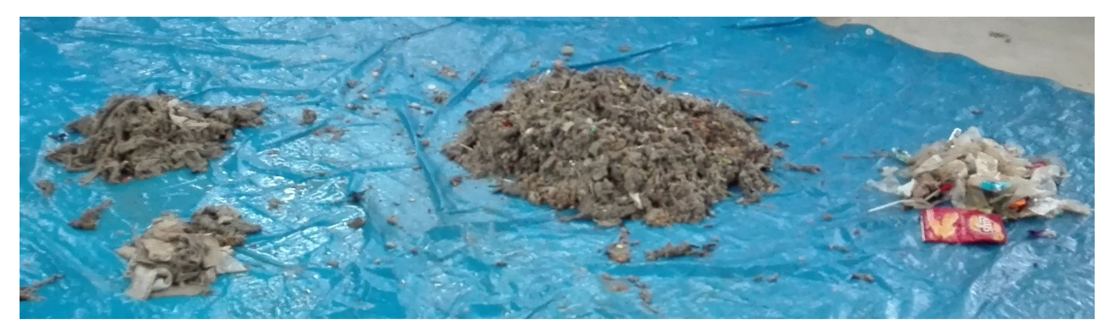
Figure 3.
Gross solids sample removed in pretreatment at Villapérez WWTP.

Figure 4.
Principal component analysis (PCA) projection of the initial data set.

Figure 5.
Analysis of results in the training phase.

Figure 6.
Cumulative distribution of the percentage of success of the model versus allowed error.

Figure 7.
Analysis of results in the testing phase.


Table 1.
Design parameters of the Villapérez wastewater treatment plant (Asturias, Spain).
| Parameter | Input | Output |
|---|---|---|
| Maximum inflow (rainy weather) | 8.50 m3/s | |
| Maximum inflow (dry weather) | 2.89 m3/s | |
| Five-day biological oxygen demand (BOD5) | 418.00 mg/L | 5 mg/L |
| Chemical oxygen demand (COD) | 652.00 mg/L | 30 mg/L |
| Total suspended solids (TSS) | 329.00 mg/L | 10 mg/L |
| Total Kjeldahl nitrogen (N-NTK) | 47.40 mg/L | 4 mg/L |
| Total phosphorus (Pt) | 6.50 mg/L | 0.5 mg/L |
Table 2.
Composition of gross solids samples from pretreatment at Villapérez WWTP.
| Sample | Total Wet Weight | Wipes | Plastics | Hygiene Products | Organic Material | ||||
|---|---|---|---|---|---|---|---|---|---|
| kg | kg | % | kg | % | kg | % | kg | % | |
| 1 | 42.21 | 13.82 | 30.57 | 0.54 | 1.19 | 1.32 | 2.92 | 29.53 | 65.32 |
| 2 | 43.61 | 12.07 | 27.68 | 0.49 | 1.12 | 1.62 | 3.71 | 29.43 | 67.48 |
| 3 | 9.25 | 2.28 | 24.56 | 0.01 | 0.11 | 0.60 | 6.49 | 6.36 | 68.76 |
Table 3.
Statistical description of the variables.
| Variable | Description | Unit | Mean | Standard Deviation | Min | Max |
|---|---|---|---|---|---|---|
| GrossSolids | Gross solids | ton | 2.96 | 0.79 | 1.42 | 5.44 |
| Interval | Time interval | h | 123.40 | 468.56 | 1.28 | 6023.36 |
| PDwR | Previous days without rain | day | 1.15 | 2.69 | 0.00 | 20.41 |
| MxDwR | Maximum previous days without rain in the time interval | day | 2.86 | 3.48 | 0.01 | 20.68 |
| Vol | Water volume | m3 | 398,312.01 | 407,147.11 | 4254.39 | 2,600,377.05 |
| PrecipTotal | Total precipitation | m3 | 7.57 | 12.37 | 0.00 | 86.50 |
| MaxpH | Maximum pH | 7.99 | 0.66 | 6.44 | 11.65 | |
| MedConductivity | Medium conductivity | µS/cm | 926.74 | 240.99 | 256.57 | 1578.82 |
| MedFlow | Medium flow | m3/h | 4853.96 | 2404.04 | 2382.21 | 14,195.72 |
| Month | Month | 5.51 | 3.19 | 1.00 | 12.00 | |
| Week | Week | 22.21 | 14.04 | 1.00 | 52.00 | |
| TempExtMed | Medium ambient temperature | °C | 11.80 | 4.53 | 3.10 | 24.60 |
| TempExtMax | Maximum ambient temperature | °C | 16.05 | 5.42 | 4.20 | 31.50 |
| TempExtMin | Minimum ambient temperature | °C | 8.49 | 4.39 | 0.70 | 19.20 |
| DayYear | Day of the year | 151.98 | 98.53 | 2.00 | 363.00 | |
| DayWeek | Day of the week | 3.18 | 1.71 | 1.00 | 6.00 | |
| MedRH | Medium relative humidity | % | 78.91 | 9.07 | 46.17 | 96.81 |
| MaxSolarRadiation | Maximum solar radiation | W/m2 | 44.89 | 79.48 | 0.77 | 532.98 |
| AtmosphericPressureMax | Maximum atmospheric pressure | millibars | 1004.52 | 7.85 | 972.41 | 1021.96 |
| MaxMedRH | Maximum relative humidity | % | 94.86 | 9.03 | 49.99 | 99.92 |
| MinMedRH | Minimum relative humidity | % | 46.84 | 18.41 | 0.00 | 92.14 |
Table 4.
Importance of variables in the model.
| Overall | % |
|---|---|
| Week | 100 |
| DayYear | 98.87 |
| PrecipTotal | 93.84 |
| MaxpH | 79.2 |
| MinMedRH | 76.58 |
| MedRH | 63.56 |
| TempExtMed | 60.08 |
| PDwR | 59.79 |
| MedFlow | 54.75 |
Publisher’s Note: MDPI stays neutral with regard to jurisdictional claims in published maps and institutional affiliations. |
© 2021 by the authors. Licensee MDPI, Basel, Switzerland. This article is an open access article distributed under the terms and conditions of the Creative Commons Attribution (CC BY) license (http://creativecommons.org/licenses/by/4.0/).
Share and Cite
MDPI and ACS Style
Mateo Pérez, V.; Mesa Fernández, J.M.; Ortega Fernández, F.; Villanueva Balsera, J. Gross Solids Content Prediction in Urban WWTPs Using SVM. Water 2021, 13, 442. https://doi.org/10.3390/w13040442
AMA Style
Mateo Pérez V, Mesa Fernández JM, Ortega Fernández F, Villanueva Balsera J. Gross Solids Content Prediction in Urban WWTPs Using SVM. Water. 2021; 13(4):442. https://doi.org/10.3390/w13040442
Chicago/Turabian StyleMateo Pérez, Vanesa, José Manuel Mesa Fernández, Francisco Ortega Fernández, and Joaquín Villanueva Balsera. 2021. "Gross Solids Content Prediction in Urban WWTPs Using SVM" Water 13, no. 4: 442. https://doi.org/10.3390/w13040442
Note that from the first issue of 2016, this journal uses article numbers instead of page numbers. See further details here.