
Study on Hydrologic Effects of Land Use Change Using a Distributed Hydrologic Model in the Dynamic Land Use Mode

Abstract
:1. Introduction
2. Materials
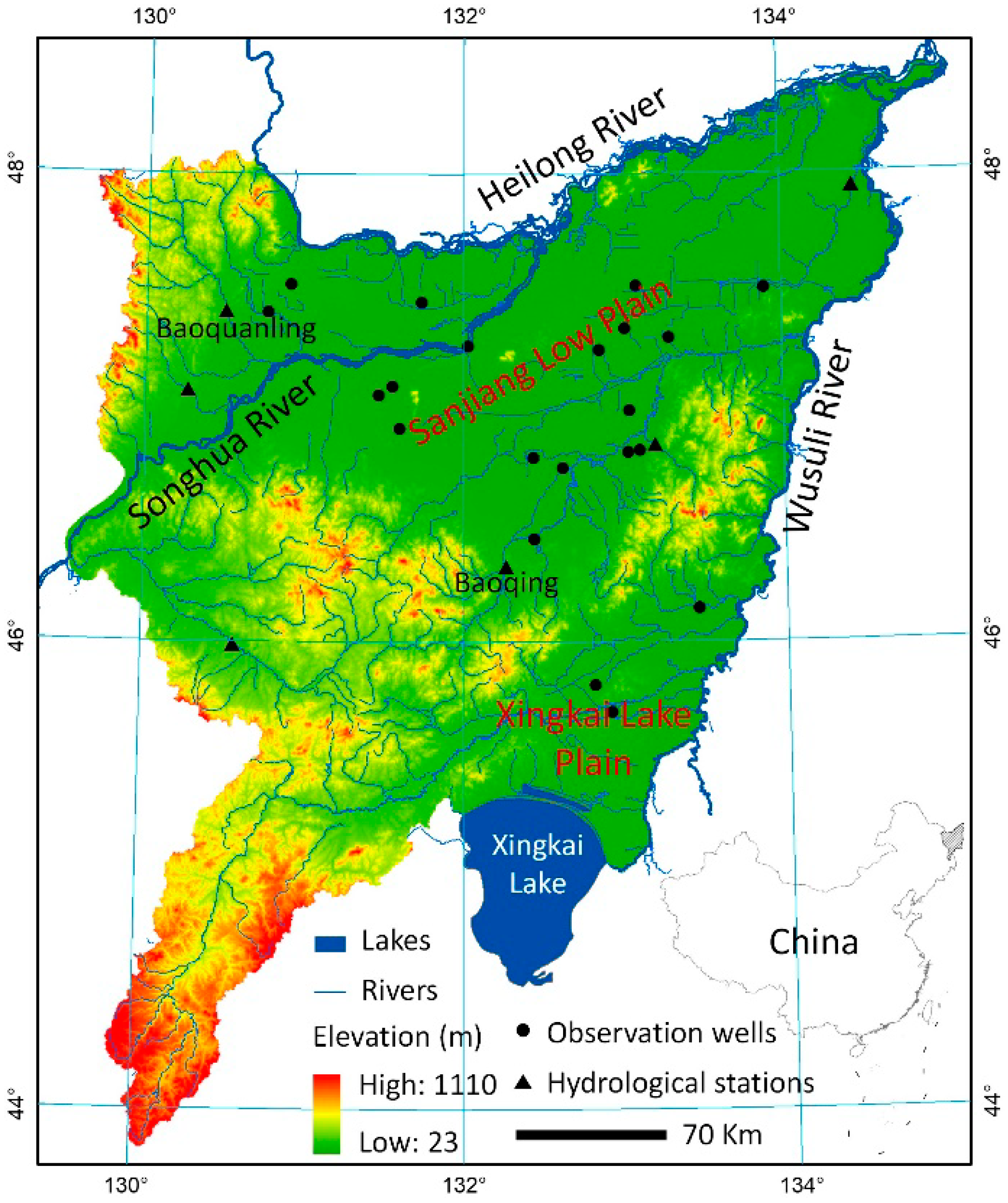
2.1. Study Area
2.2. Data
2.2.1. Basic Spatial Data
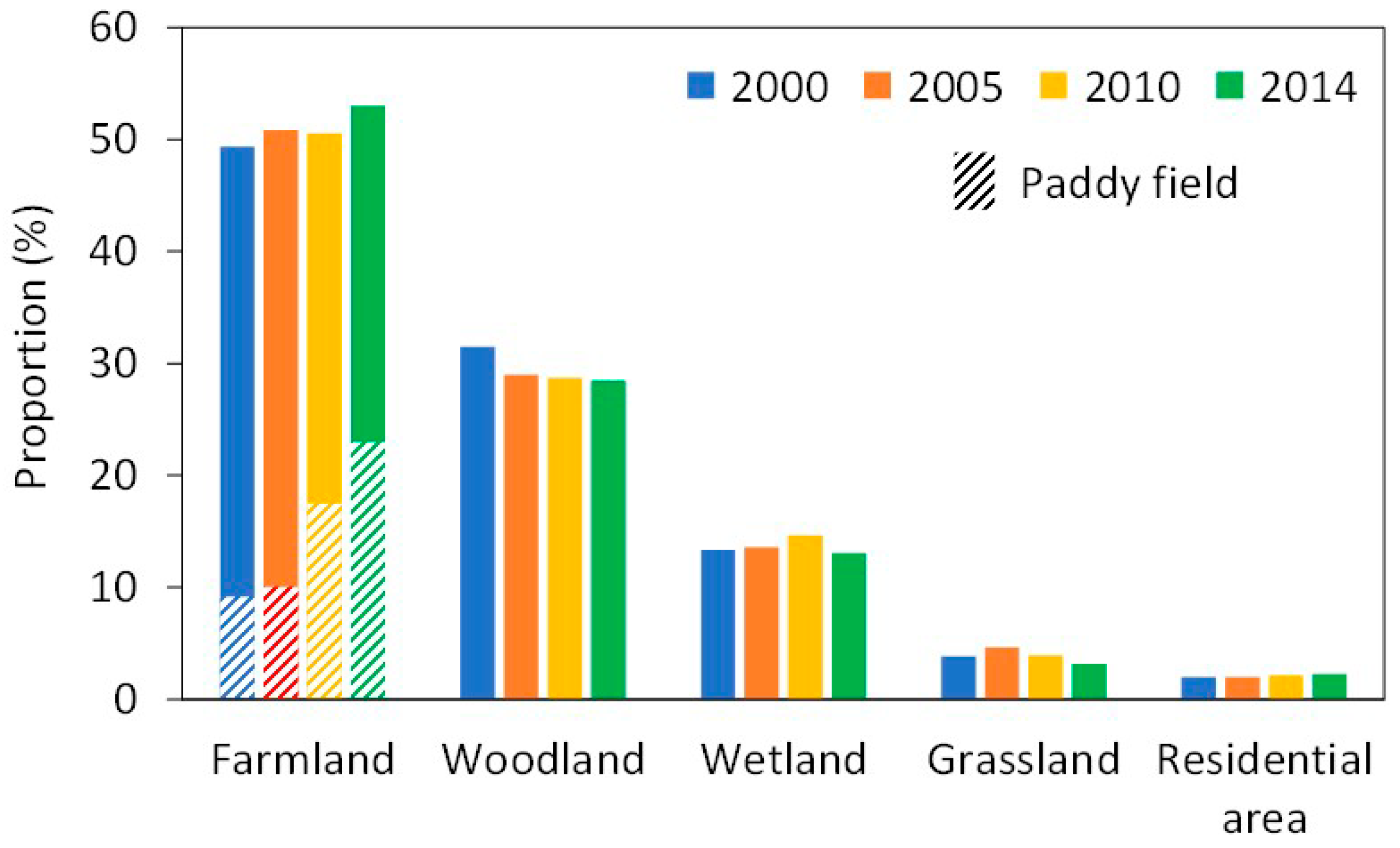
2.2.2. Land Use Data
3. Methods
3.1. Structure and Framework of MODCYCLE
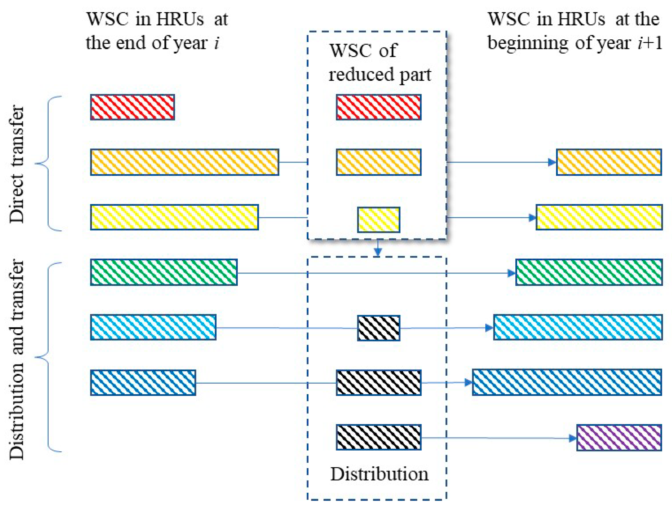
3.2. Dynamic Land Use Mode
3.3. Model Performance Evaluation
3.4. Analysis of Land Use Change and Its Hydrological Effect
4. Results
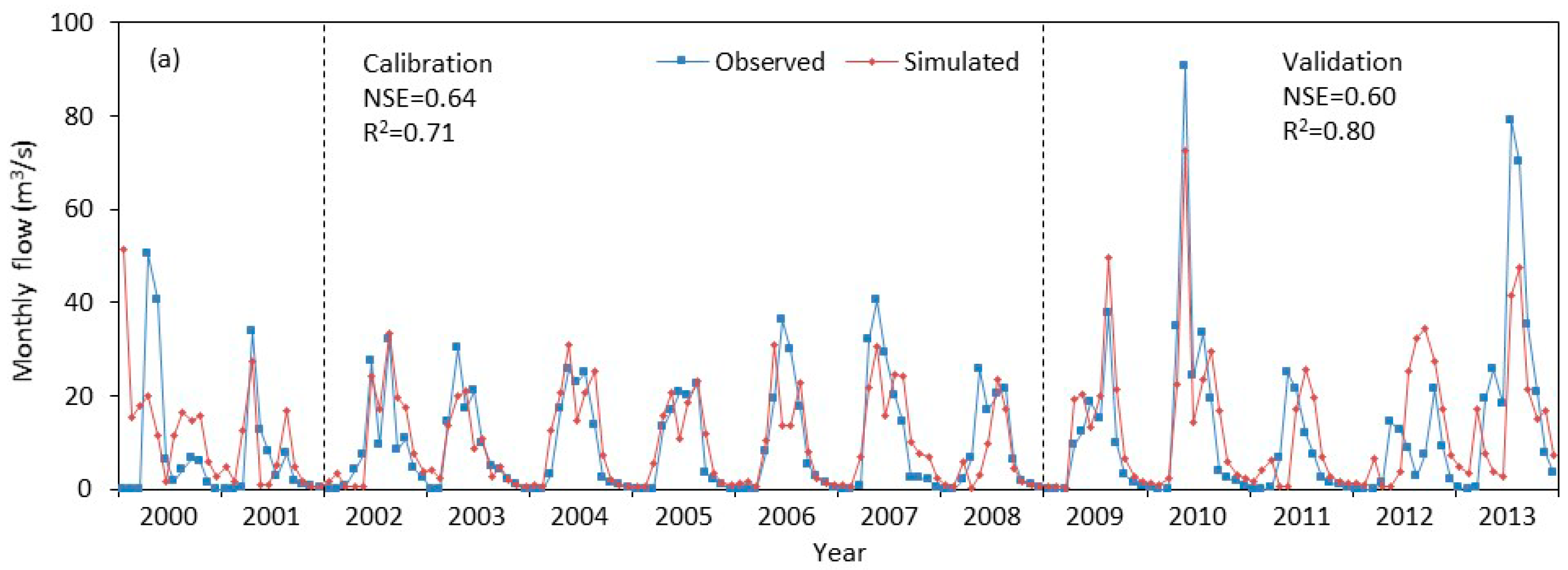
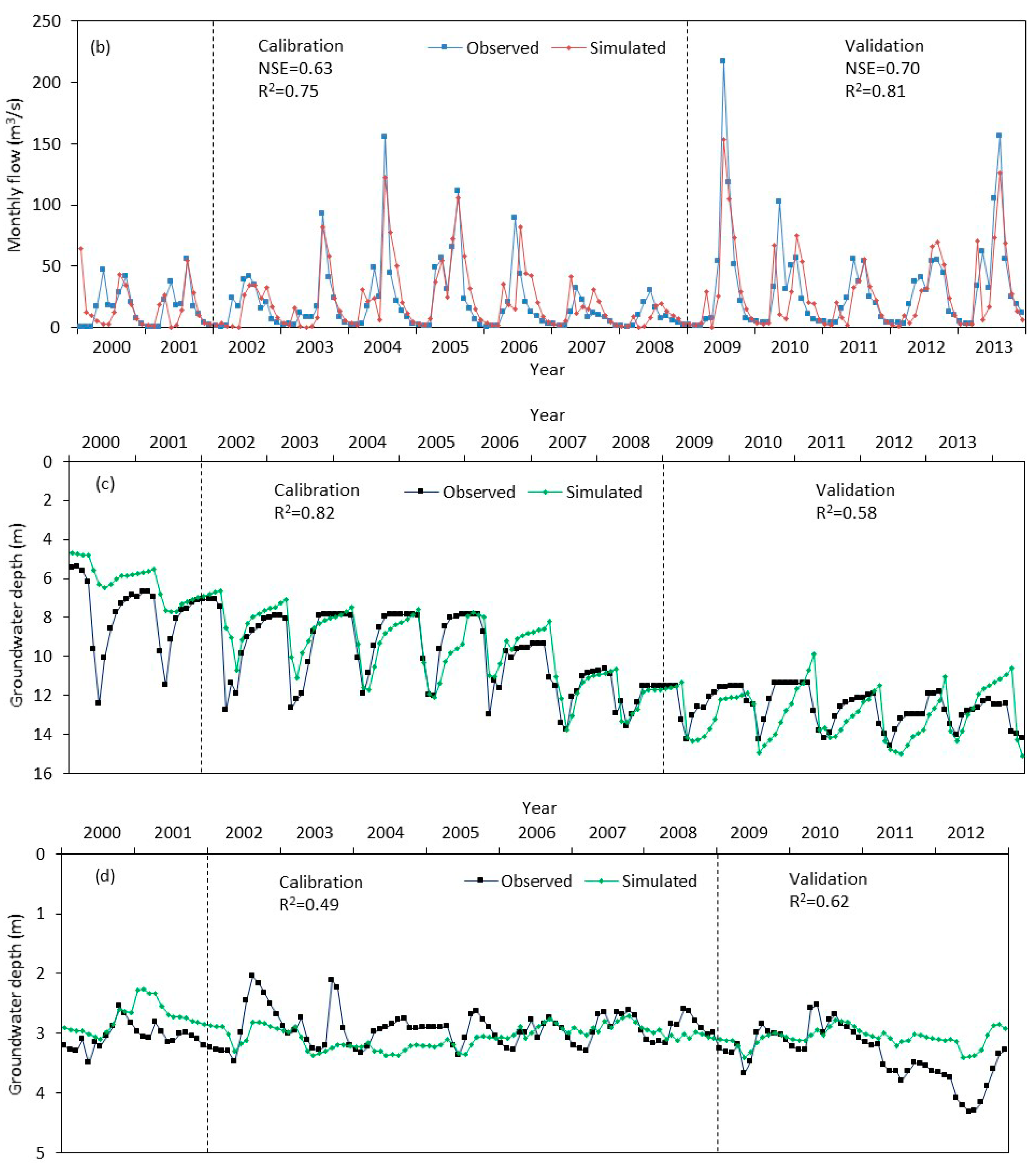
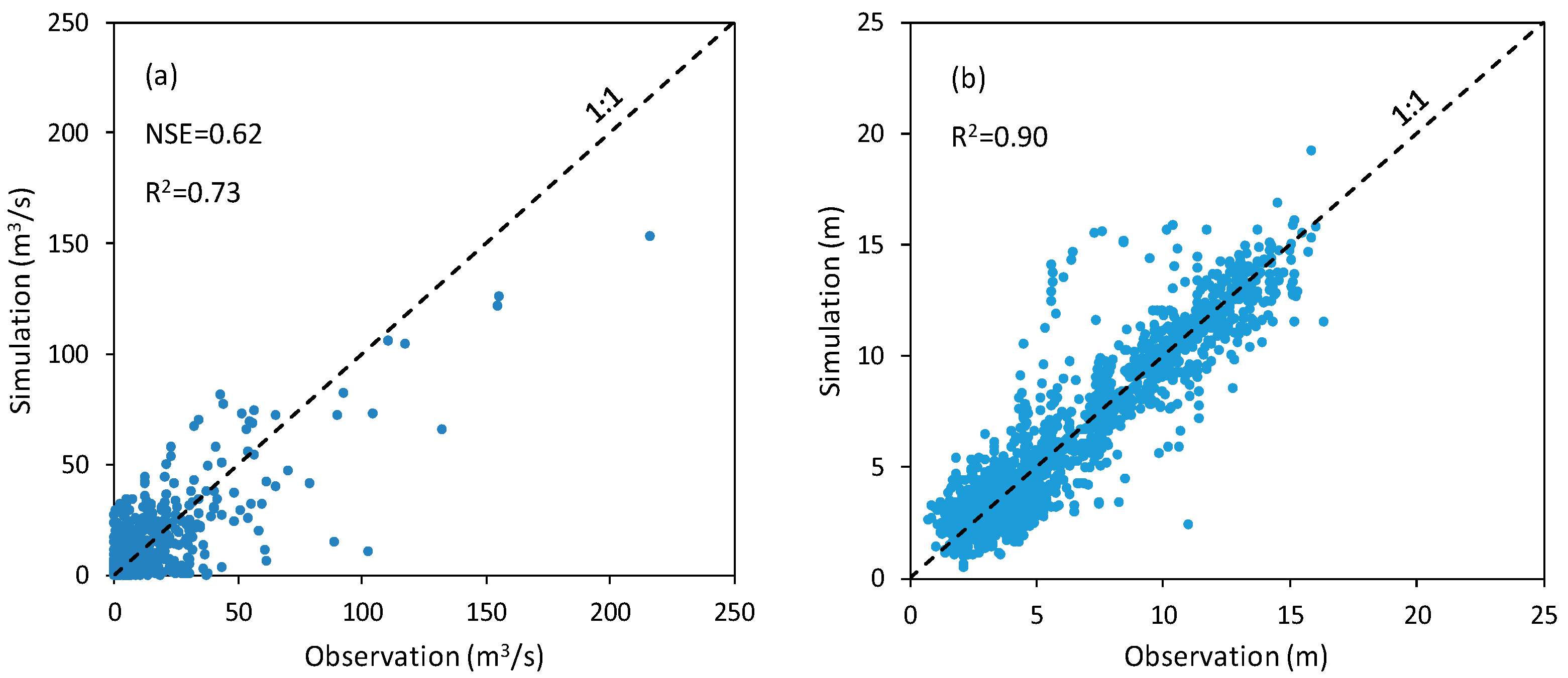
4.1. Model Calibration and Validation
4.2. Hydrologic Effects of Land Use Change
4.2.1. Comparison of the Two Land Use Change Patterns
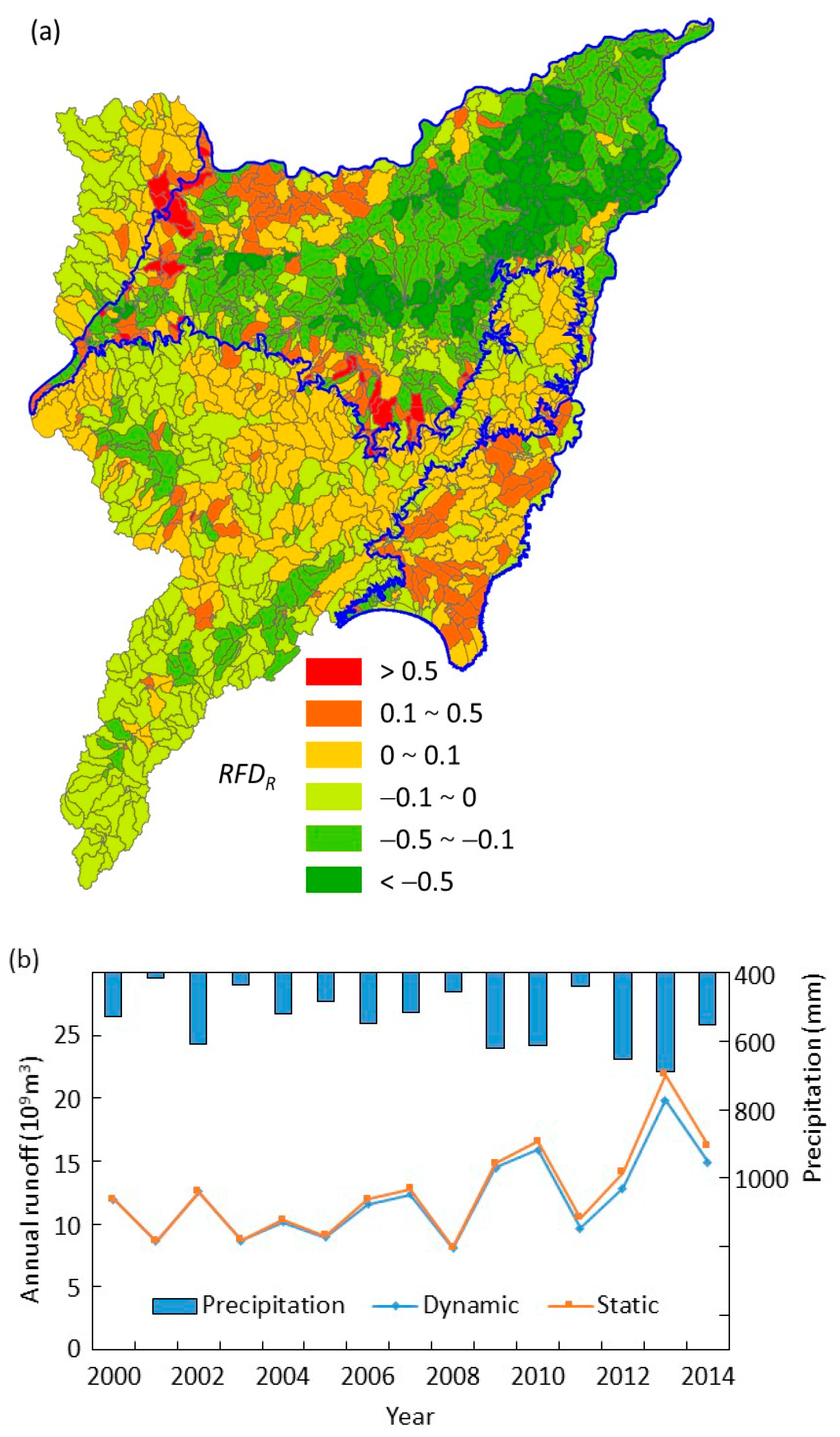
4.2.2. Runoff Effect
4.2.3. Evapotranspiration Effect
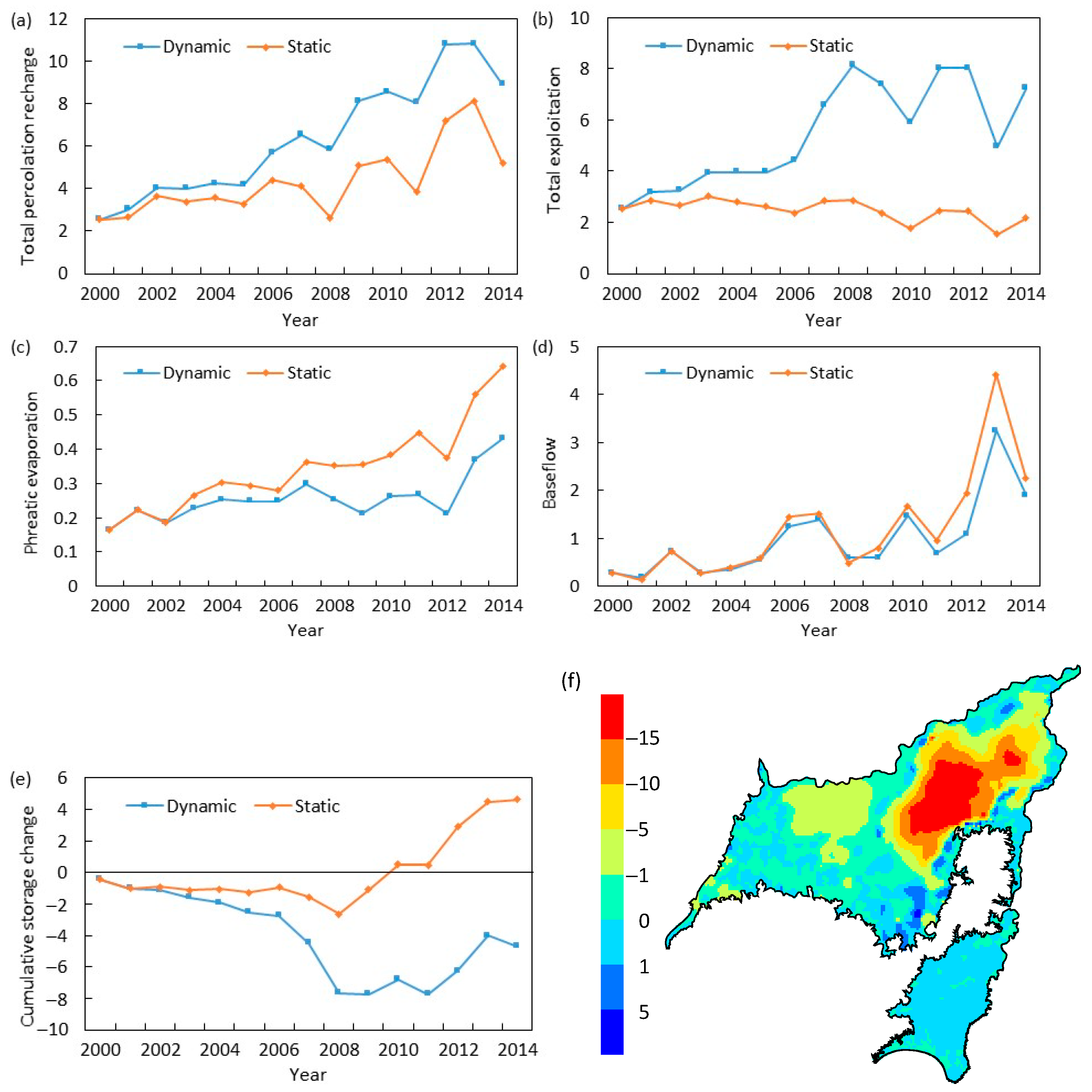
4.2.4. Groundwater Effect
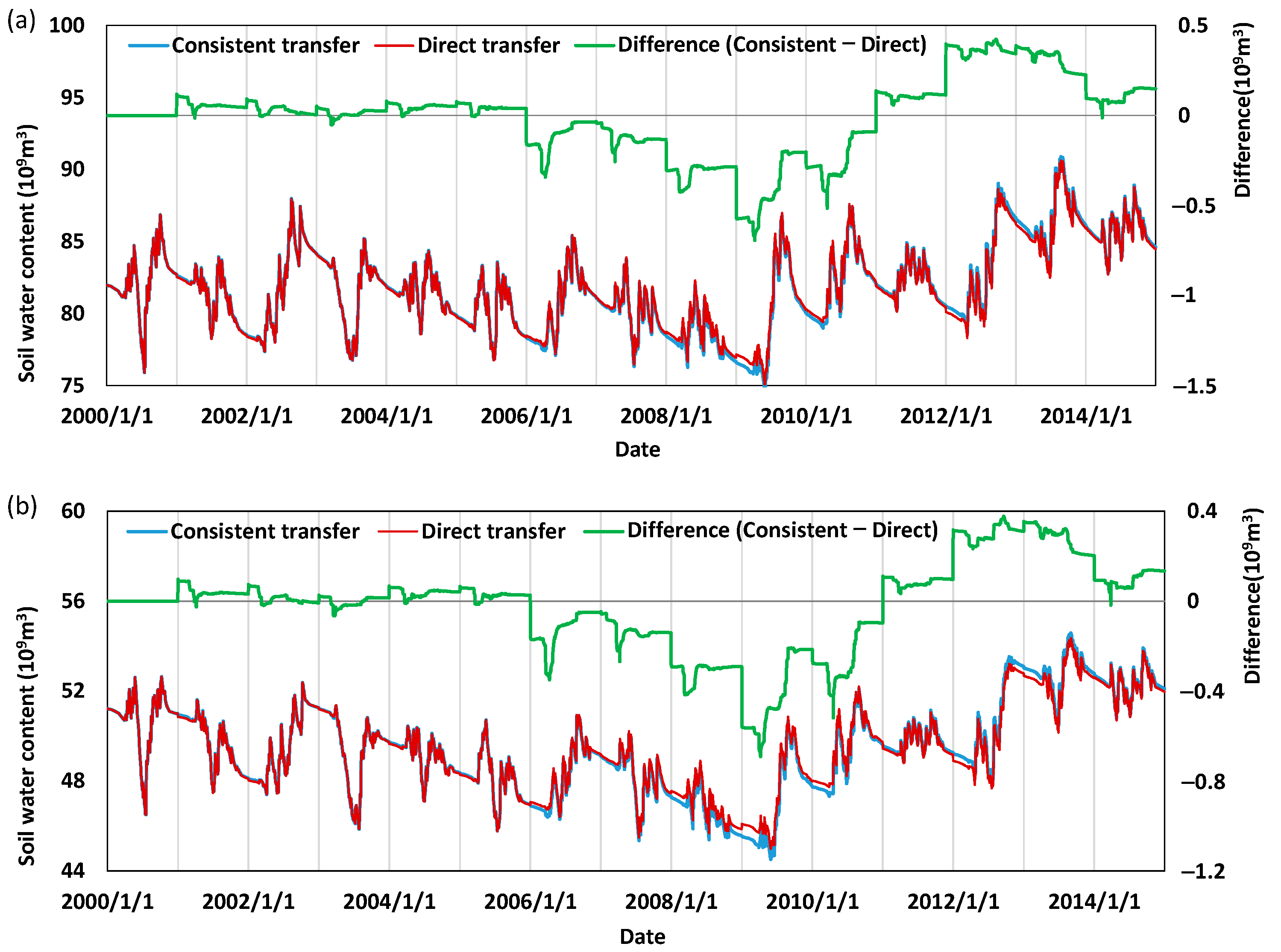
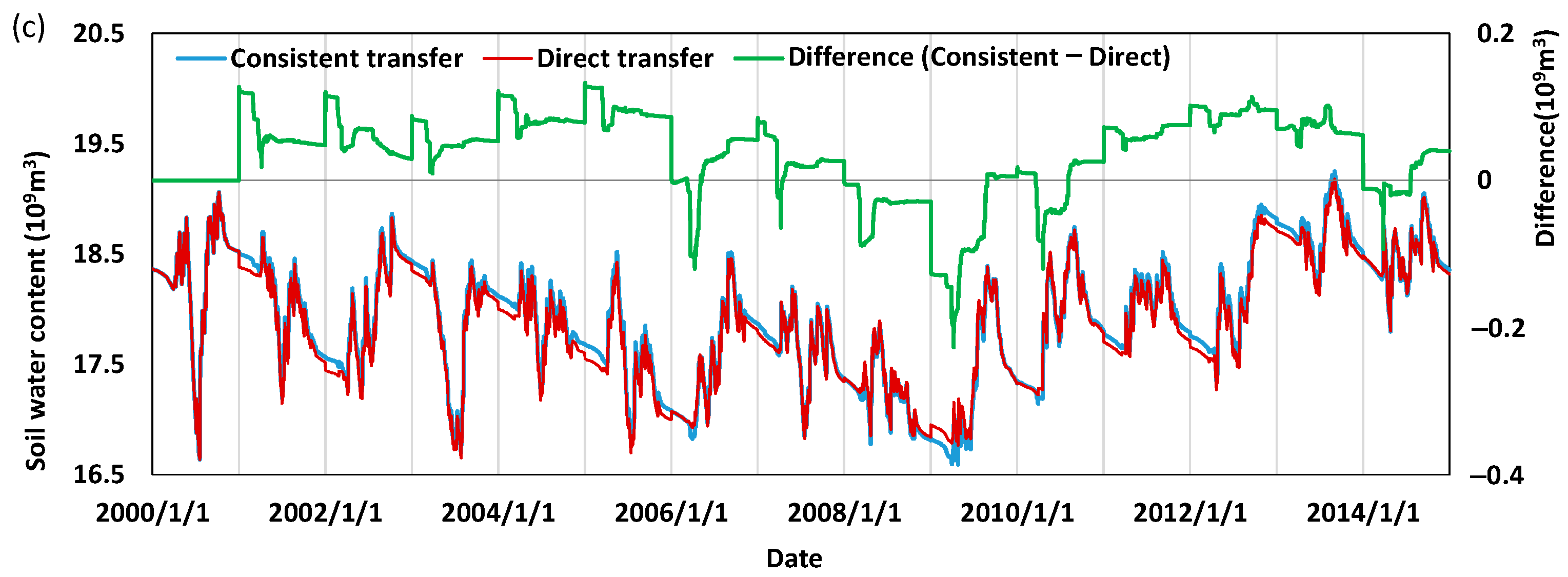
4.3. Difference between Consistent and Direct Transfer of HRU Water Storage
5. Discussion
6. Conclusions
Supplementary Materials
Author Contributions
Funding
Institutional Review Board Statement
Informed Consent Statement
Data Availability Statement
Conflicts of Interest
References
- Foley, J.A.; DeFries, R.; Asner, G.P.; Barford, C.; Bonan, G.; Carpenter, S.R.; Chapin, F.S.; Coe, M.T.; Daily, G.C.; Gibbs, H.K.; et al. Global consequences of land use. Science 2005, 309, 570–574. [Google Scholar] [CrossRef] [PubMed] [Green Version]
- Liu, M.; Tian, H. China’s land cover and land use change from 1700 to 2005: Estimations from high-resolution satellite data and historical archives. Glob. Biogeochem. Cycle 2010, 24. [Google Scholar] [CrossRef]
- Sajikumar, N.; Remya, R.S. Impact of land cover and land use change on runoff characteristics. J. Environ. Manag. 2015, 161, 460–468. [Google Scholar] [CrossRef] [PubMed]
- Sterling, S.M.; Ducharne, A.; Polcher, J. The impact of global land-cover change on the terrestrial water cycle. Nat. Clim. Chang. 2012, 3, 385–390. [Google Scholar] [CrossRef]
- Gupta, S.C.; Kessler, A.C.; Brown, M.K.; Zvomuya, F. Climate and agricultural land use change impacts on streamflow in the upper midwestern United States. Water Resour. Res. 2015, 51, 5301–5317. [Google Scholar] [CrossRef]
- Ghaffari, G.; Keesstra, S.; Ghodousi, J.; Ahmadi, H. SWAT-simulated hydrological impact of land-use change in the Zanjanrood Basin, Northwest Iran. Hydrol. Process. 2010, 24, 892–903. [Google Scholar] [CrossRef]
- Neupane, R.P.; Kumar, S. Estimating the effects of potential climate and land use changes on hydrologic processes of a large agriculture dominated watershed. J. Hydrol. 2015, 529, 418–429. [Google Scholar] [CrossRef]
- Jacobson, C.R. Identification and quantification of the hydrological impacts of imperviousness in urban catchments: A review. J. Environ. Manag. 2011, 92, 1438–1448. [Google Scholar] [CrossRef]
- Dias, L.C.P.; Macedo, M.N.; Costa, M.H.; Coe, M.T.; Neill, C. Effects of land cover change on evapotranspiration and streamflow of small catchments in the Upper Xingu River Basin, Central Brazil. J. Hydrol. Reg. Stud. 2015, 4, 108–122. [Google Scholar] [CrossRef] [Green Version]
- Dawes, W.; Ali, R.; Varma, S.; Emelyanova, I.; Hodgson, G.; McFarlane, D. Modelling the effects of climate and land cover change on groundwater recharge in south-west Western Australia. Hydrol. Earth Syst. Sci. 2012, 16, 2709–2722. [Google Scholar] [CrossRef] [Green Version]
- Zhang, Y.K.; Schilling, K.E. Increasing streamflow and baseflow in Mississippi River since the 1940s: Effect of land use change. J. Hydrol. 2006, 324, 412–422. [Google Scholar] [CrossRef]
- Valentin, C.; Agus, F.; Alamban, R.; Boosaner, A.; Bricquet, J.P.; Chaplot, V.; de Guzman, T.; de Rouw, A.; Janeau, J.L.; Orange, D.; et al. Runoff and sediment losses from 27 upland catchments in Southeast Asia: Impact of rapid land use changes and conservation practices. Agric. Ecosyst. Environ. 2008, 128, 225–238. [Google Scholar] [CrossRef]
- Gebrehiwot, S.G.; Taye, A.; Bishop, K. Forest cover and stream flow in a headwater of the Blue Nile: Complementing observational data analysis with community perception. Ambio 2010, 39, 284–294. [Google Scholar] [CrossRef] [Green Version]
- Zhang, X.; Zhang, L.; Zhao, J.; Rustomji, P.; Hairsine, P. Responses of streamflow to changes in climate and land use/cover in the Loess Plateau, China. Water Resour. Res. 2008, 44. [Google Scholar] [CrossRef]
- Schoonover, J.E.; Lockaby, B.G.; Helms, B.S. Impacts of land cover on stream hydrology in the West Georgia Piedmont, USA. J. Environ. Qual. 2006, 35, 2123–2131. [Google Scholar] [CrossRef] [PubMed]
- Dwarakish, G.S.; Ganasri, B.P. Impact of land use change on hydrological systems: A review of current modeling approaches. Cogent. Geosci. 2015, 1, 1–18. [Google Scholar] [CrossRef]
- Wagner, P.D.; Bhallamudi, S.M.; Narasimhan, B.; Kumar, S.; Fohrer, N.; Fiener, P. Comparing the effects of dynamic versus static representations of land use change in hydrologic impact assessments. Environ. Modell. Softw. 2017, 122, 103987. [Google Scholar] [CrossRef]
- Alvarenga, L.A.; de Mello, C.R.; Colombo, A.; Cuartas, L.A.; Bowling, L.C. Assessment of land cover change on the hydrology of a Brazilian headwater watershed using the Distributed Hydrology–Soil–Vegetation Model. Catena 2016, 143, 7–17. [Google Scholar] [CrossRef]
- Yang, L.; Feng, Q.; Yin, Z.; Wen, X.; Si, J.; Li, C.; Deo, R.C. Identifying separate impacts of climate and land use/cover change on hydrological processes in upper stream of Heihe River, Northwest China. Hydrol. Process. 2017, 31, 1100–1112. [Google Scholar] [CrossRef]
- Öztürk, M.; Copty, N.K.; Saysel, A.K. Modeling the impact of land use change on the hydrology of a rural watershed. J. Hydrol. 2013, 497, 97–109. [Google Scholar] [CrossRef]
- Brath, A.; Montanari, A.; Moretti, G. Assessing the effect on flood frequency of land use change via hydrological simulation (with uncertainty). J. Hydrol. 2006, 324, 141–153. [Google Scholar] [CrossRef]
- Choi, W.; Deal, B.M. Assessing hydrological impact of potential land use change through hydrological and land use change modeling for the Kishwaukee River basin (USA). J. Environ. Manag. 2008, 88, 1119–1130. [Google Scholar] [CrossRef] [PubMed]
- Chen, Y.; Xu, Y.; Yin, Y. Impacts of land use change scenarios on storm-runoff generation in Xitiaoxi basin, China. Quat. Int. 2009, 208, 121–128. [Google Scholar] [CrossRef]
- Schilling, K.E.; Jha, M.K.; Zhang, Y.; Gassman, P.W.; Wolter, C.F. Impact of land use and land cover change on the water balance of a large agricultural watershed: Historical effects and future directions. Water Resour. Res. 2008, 44. [Google Scholar] [CrossRef]
- Elfert, S.; Bormann, H. Simulated impact of past and possible future land use changes on the hydrological response of the Northern German lowland ‘Hunte’ catchment. J. Hydrol. 2010, 383, 245–255. [Google Scholar] [CrossRef]
- Li, Z.; Liu, W.-z.; Zhang, X.-c.; Zheng, F.-l. Impacts of land use change and climate variability on hydrology in an agricultural catchment on the Loess Plateau of China. J. Hydrol. 2009, 377, 35–42. [Google Scholar] [CrossRef]
- Im, S.; Kim, H.; Kim, C.; Jang, C. Assessing the impacts of land use changes on watershed hydrology using MIKE SHE. Environ. Geol. 2008, 57, 231–239. [Google Scholar] [CrossRef]
- Nie, W.; Yuan, Y.; Kepner, W.; Nash, M.S.; Jackson, M.; Erickson, C. Assessing impacts of Landuse and Landcover changes on hydrology for the upper San Pedro watershed. J. Hydrol. 2011, 407, 105–114. [Google Scholar] [CrossRef]
- Matese, A.; Toscano, P.; Di Gennaro, F.S.; Genesio, L.; Vaccari, P.F.; Primicerio, J.; Belli, C.; Zaldei, A.; Bianconi, R.; Gioli, B. Intercomparison of UAV, aircraft and satellite remote sensing platforms for precision viticulture. Remote Sens. 2015, 7, 2971–2990. [Google Scholar] [CrossRef] [Green Version]
- Pajares, G. Overview and current status of remote sensing applications based on unmanned aerial vehicles (UAVs). Photogramm. Eng. Remote Sens. 2015, 81, 281–329. [Google Scholar] [CrossRef] [Green Version]
- Toth, C.; Jóźków, G. Remote sensing platforms and sensors: A survey. ISPRS J. Photogramm. Remote Sens. 2016, 115, 22–36. [Google Scholar] [CrossRef]
- Neitsch, S.L.; Arnold, J.G.; Kiniry, J.R.; Srinivasan, R.; Williams, J.R. Soil and Water Assessment Tool Input/Output File Documentation, Version 2005; Grassland, Soil and Water Research Laboratory, Agricultural Research Service and Blackland Research Center, Texas Agricultural Experiment Station: College Station, TX, USA, 2004; Available online: https://swat.tamu.edu/media/1291/SWAT2005io.pdf (accessed on 8 February 2021).
- Niehoff, D.; Fritsch, U.; Bronstert, A. Land-use impacts on storm-runoff generation: Scenarios of land-use change and simulation of hydrological response in a meso-scale catchment in SW-Germany. J. Hydrol. 2002, 267, 80–93. [Google Scholar] [CrossRef]
- Liang, X.; Lettenmaier, D.P.; Wood, E.F.; Burges, S.J. A simple hydrologically based model of land surface water and energy fluxes for general circulation models. J. Geophys. Res. Atmos. 1994, 99, 14415–14428. [Google Scholar] [CrossRef]
- Chu, H.; Lin, Y.; Huang, C.; Hsu, C.; Chen, H. Modelling the hydrologic effects of dynamic land-use change using a distributed hydrologic model and a spatial land-use allocation model. Hydrol. Process. 2010, 24, 2538–2554. [Google Scholar] [CrossRef]
- Chiang, L.; Chaubey, I.; Gitau, M.W.; Arnold, J.G. Differentiating impacts of land use changes from pasture management in a CEAP watershed using the SWAT model. Trans. ASABE 2010, 53, 1569–1584. [Google Scholar] [CrossRef]
- Pai, N.; Saraswat, D. SWAT2009_LUC: A tool to activate the land use change module in SWAT 2009. Trans. ASABE 2011, 54, 1649–1658. [Google Scholar] [CrossRef]
- Wagner, P.D.; Bhallamudi, S.M.; Narasimhan, B.; Kantakumar, L.N.; Sudheer, K.P.; Kumar, S.; Schneider, K.; Fiener, P. Dynamic integration of land use changes in a hydrologic assessment of a rapidly developing Indian catchment. Sci. Total Environ. 2016, 539, 153–164. [Google Scholar] [CrossRef]
- Teklay, A.; Dile, Y.T.; Setegn, S.G.; Demissie, S.S.; Asfaw, D.H. Evaluation of static and dynamic land use data for watershed hydrologic process simulation: A case study in Gummara watershed, Ethiopia. Catena 2019, 172, 65–75. [Google Scholar] [CrossRef]
- Wang, Q.; Liu, R.; Men, C.; Guo, L.; Miao, Y. Effects of dynamic land use inputs on improvement of SWAT model performance and uncertainty analysis of outputs. J. Hydrol. 2018, 563, 874–886. [Google Scholar] [CrossRef]
- Lee, D.; Han, J.H.; Park, M.J.; Engel, B.A.; Kim, J.; Lim, K.J.; Jang, W.S. Development of advanced web-based SWAT LUC system considering yearly land use changes and recession curve characteristics. Ecol. Eng. 2019, 128, 39–47. [Google Scholar] [CrossRef]
- Van Roosmalen, L.; Sonnenborg, T.O.; Jensen, K.H. Impact of climate and land use change on the hydrology of a large-scale agricultural catchment. Water Resour. Res. 2009, 45. [Google Scholar] [CrossRef] [Green Version]
- Arnold, J.G.; Kiniry, J.R.; Srinivasan, R.; Williams, J.R.; Haney, E.B.; Neitsch, S.L. Soil and Water Assessment Tool Input/Output File Documentation, Version 2009; Grassland, Soil and Water Research Laboratory, Agricultural Research Service and Blackland Research Center, Texas Agricultural Experiment Station; Texas Water Resources Institute Technical Report No. 365; Texas A & M University System: College Station, TX, USA, 2011; Available online: https://swat.tamu.edu/media/19754/swat-io-2009.pdf (accessed on 8 February 2021).
- Arnold, J.G.; Gassman, P.W.; White, M.J. New Developments in the SWAT Ecohydrology Model. In 21st Century Watershed Technology: Improving Water Quality and Environment Conference, Guacimo, Costa Rica, 21–24 February 2010; American Society of Agricultural and Biological Engineers: St. Joseph, MI, USA, 2010; Available online: https://elibrary.asabe.org/abstract.asp?aid=29393 (accessed on 8 February 2021).
- Aghsaei, H.; Mobarghaee Dinan, N.; Moridi, A.; Asadolahi, Z.; Delavar, M.; Fohrer, N.; Wagner, P.D. Effects of dynamic land use/land cover change on water resources and sediment yield in the Anzali wetland catchment, Gilan, Iran. Sci. Total Environ. 2020, 712, 136449. [Google Scholar] [CrossRef]
- Lu, C.; Qin, D.; Zhang, J.; Wang, R. MODCYCLE–An object oriented modularized hydrological model I. Theory and development. J. Hydraul. Eng. 2012, 43, 1135–1145. [Google Scholar]
- Wang, J.; Lu, C.; Sun, Q.; Xiao, W.; Cao, G.; Li, H.; Yan, L.; Zhang, B. Simulating the hydrologic cycle in coal mining subsidence areas with a distributed hydrologic model. Sci. Rep. 2017, 7, 39983. [Google Scholar] [CrossRef] [Green Version]
- Sun, Q.; Lu, C.; Luan, Q.; Li, H.; Wang, L. Simulation and analysis of grassland ecosystem dependence on phreatic water in semi-arid areas. Trans. Chin. Soc. Agric. Eng. 2013, 29, 118–127. [Google Scholar]
- Gao, X.; Wang, J.; Wu, P.; Zhao, Y.; Zhao, X.; He, F. Evaluation of soil water availability (SWA) based on hydrological modelling in arid and semi-arid areas: A case study in Handan City, China. Water 2016, 8, 360. [Google Scholar] [CrossRef]
- Gao, X.; Lu, C.; Luan, Q.; Zhang, S.; Liu, J.; Han, D. Mapping farmland-soil moisture at a regional scale using a distributed hydrological model: Case study in the North China Plain. J. Irrig. Drain. Eng. 2016, 14, 04016029. [Google Scholar] [CrossRef]
- Lu, C.; Sun, Q.; Cao, G.; Luan, Q.; Yan, L.; Zhang, B.; Li, T.; Lai, B. Soil water transformation regularity of farmland for typical crop in Beijing–Tianjin–Hebei region: Experimental and simulating analyses. In Proceedings of the MATEC Web Conf EDP, Sciences, Les Ulis, France, 12–14 October 2018; Available online: https://doi.org/10.1051/matecconf/201824601061 (accessed on 8 February 2021).
- Zhang, B.; Lu, C.; Wang, J.; Sun, Q.; He, X.; Cao, G.; Zhao, Y.; Yan, L.; Gong, B. Using storage of coal-mining subsidence area for minimizing flood. J. Hydrol. 2019, 572, 571–581. [Google Scholar] [CrossRef]
- Zhang, J.; Lu, C.; Qin, D.; Wang, R. MODCYCLE–An object oriented modularized hydrological model II. Application. J. Hydraul. Eng. 2012, 43, 1287–1295. [Google Scholar]
- Liu, X.; An, Y.; Dong, G.; Jiang, M. Land use and landscape pattern changes in the Sanjiang Plain, Northeast China. Forests 2018, 9, 637. [Google Scholar] [CrossRef] [Green Version]
- Dong, G.; Bai, J.; Yang, S.; Wu, L.; Cai, M.; Zhang, Y.; Luo, Y.; Wang, Z. The impact of land use and land cover change on net primary productivity on China’s Sanjiang Plain. Environ. Earth Sci. 2015, 74, 2907–2917. [Google Scholar] [CrossRef]
- Durán, A.; Morrás, H.; Studdert, G.; Liu, X. Distribution, properties, land use and management of Mollisols in South America. Chin. Geogr. Sci. 2011, 21, 511. [Google Scholar] [CrossRef]
- Gleeson, T.; Manning, A.H. Regional groundwater flow in mountainous terrain: Three-dimensional simulations of topographic and hydrogeologic controls. Water Resour. Res. 2008, 44, 1–16. [Google Scholar] [CrossRef]
- Welch, L.A.; Allen, D.M. Consistency of groundwater flow patterns in mountainous topography: Implications for valley bottom water replenishment and for defining groundwater flow boundaries. Water Resour. Res. 2012, 48. [Google Scholar] [CrossRef] [Green Version]
- Moriasi, D.N.; Gitau, M.W.; Pai, N.; Daggupati, P. Hydrologic and water quality models: Performance measures and evaluation criteria. Trans. ASABE 2015, 58, 1763–1785. [Google Scholar]
- Nash, J.E.; Sutcliffe, J.V. River flow forecasting through conceptual models part I–A discussion of principles. J. Hydrol. 1970, 10, 282–290. [Google Scholar] [CrossRef]
- Willmott, C.J. On the validation of models. Phys. Geogr. 1981, 2, 184–194. [Google Scholar] [CrossRef]
- Gupta, H.V.; Sorooshian, S.; Yapo, P.O. Status of automatic calibration for hydrologic models: Comparison with multilevel expert calibration. J. Hydrol. Eng. 1999, 4, 135–143. [Google Scholar] [CrossRef]
- Cao, W.; Bowden, W.B.; Davie, T.; Fenemor, A. Multi-variable and multi-site calibration and validation of SWAT in a large mountainous catchment with high spatial variability. Hydrol. Process. 2006, 20, 1057–1073. [Google Scholar] [CrossRef]
- Immerzeel, W.W.; Droogers, P. Calibration of a distributed hydrological model based on satellite evapotranspiration. J. Hydrol. 2008, 349, 411–424. [Google Scholar] [CrossRef]
- Motovilov, Y.G.; Gottschalk, L.; Engeland, K.; Rodhe, A. Validation of a distributed hydrological model against spatial observations. Agric. For. Meteorol. 1999, 98–99, 257–277. [Google Scholar] [CrossRef]
- Boyle, D.P.; Gupta, H.V.; Sorooshian, S. Toward improved calibration of hydrologic models: Combining the strengths of manual and automatic methods. Water Resour. Res. 2000, 36, 3663–3674. [Google Scholar] [CrossRef]
- Kim, S.M.; Benham, B.L.; Brannan, K.M.; Zeckoski, R.W.; Doherty, J. Comparison of hydrologic calibration of HSPF using automatic and manual methods. Water Resour. Res. 2007, 43. [Google Scholar] [CrossRef]
- Beven, K. Prophecy, reality and uncertainty in distributed hydrological modelling. Adv. Water Resour. 1993, 16, 41–51. [Google Scholar] [CrossRef]
- Vrugt, J.A.; Gupta, H.V.; Bouten, W.; Sorooshian, S. A Shuffled Complex Evolution Metropolis algorithm for optimization and uncertainty assessment of hydrologic model parameters. Water Resour. Res. 2003, 39. [Google Scholar] [CrossRef] [Green Version]
- Tsuchiya, R.; Kato, T.; Jeong, J.; Arnold, J.G. Development of SWAT-Paddy for Simulating Lowland Paddy Fields. Sustainability 2018, 10, 3246. [Google Scholar] [CrossRef] [Green Version]
- Zuo, Y.; Guo, Y.; Song, C.; Jin, S.; Qiao, T. Study on soil water and weat transport characteristic responses to land use change in Sanjiang Plain. Sustainability 2019, 11, 157. [Google Scholar] [CrossRef] [Green Version]
- Arnold, J.G.; Srinivasan, R.; Muttiah, R.S.; Williams, J.R. Large area hydrologic modeling and assessment part I: Model development. J. Am. Water Resour. Assoc. 1998, 34, 73–89. [Google Scholar] [CrossRef]
- Kosmas, C.; Gerontidis, S.; Marathianou, M. The effect of land use change on soils and vegetation over various lithological formations on Lesvos (Greece). Catena 2000, 40, 51–68. [Google Scholar] [CrossRef]
- Devanand, A.; Huang, M.; Lawrence, D.M.; Zarzycki, C.M.; Feng, Z.; Lawrence, P.J.; Qian, Y.; Yang, Z. Land use and land cover change strongly modulates land-atmosphere coupling and warm-season precipitation over the central United States in CESM2-VR. J. Adv. Model. Earth Syst. 2020, 12, e2019MS001925. [Google Scholar] [CrossRef]
- Beltrán-Przekurat, A.; Pielke Sr, R.A.; Eastman, J.L.; Coughenour, M.B. Modelling the effects of land-use/land-cover changes on the near-surface atmosphere in southern South America. Int. J. Climatol. 2012, 32, 1206–1225. [Google Scholar] [CrossRef] [Green Version]


| Variable | Description (Units) | Recommended Range | Actual Min./Max. Values Used | Hydrologic Process |
|---|---|---|---|---|
| Hydrologic cycle simulation | ||||
| MXSURPOND | Maximum depth of surface ponding (mm) | 0.0–150.0 | 1–100 | Runoff |
| ALPHA_BF | Baseflow alpha factor (days) | 0.0–1.0 | 0.05–0.08 | Groundwater |
| ESCO | Soil evaporation compensation factor (-) | 0.01–1.0 | 0.9–0.92 | Evaporation |
| SURLAG | Surface runoff lag coefficient (-) | 1.0–24.0 | 5.0–5.0 | Runoff |
| SOL_AWC | Available water capacity of the soil layer (-) | 0.0–1.0 | 0.01–0.25 | Soil water |
| SOL_K | Saturated hydraulic conductivity (mm/h) | 0.0–25.0 | 0.018–25 | Soil water |
| GWDMN | Threshold water level in shallow aquifer for baseflow (m) | 0.0–5.0 | 2.5–2.5 | Groundwater |
| Groundwater numerical simulation | ||||
| HY | Hydraulic conductivity (m/d) | 0.25–7.5 | Groundwater | |
| SC1 | Primary storage coefficient 1 (-) | 0.008–0.175 | Groundwater | |
| SC2 | Primary storage coefficient 2 (-) | 0.004–0.175 | Groundwater | |
| Hydrologic Fluxes and Storage Changes | Consistent | Direct |
|---|---|---|
| Recharges | ||
| Precipitation on non-surface water | 56.31 | 56.31 |
| Precipitation on surface water | 0.12 | 0.12 |
| Surface water inflow a | 46.73 | 46.73 |
| Groundwater boundary inflow | 0.00 | 0.00 |
| Outside water diversion for irrigation b | 0.75 | 0.75 |
| Outside water diversion for other water supply c | 0.75 | 0.75 |
| Total recharge | 104.65 | 104.65 |
| Discharges | ||
| Interception evaporation | 2.70 | 2.70 |
| Snow sublimation | 0.18 | 0.18 |
| Ponding evaporation | 7.34 | 7.34 |
| Soil evaporation | 23.55 | 23.58 |
| Vegetation transpiration | 11.44 | 11.43 |
| Surface water evaporation | 1.76 | 1.76 |
| Surface water outflow | 54.81 | 54.72 |
| Groundwater boundary outflow | 0.00 | 0.00 |
| Evaporation of irrigation system | 1.42 | 1.42 |
| Other water consumption d | 1.21 | 1.21 |
| Total discharge | 104.41 | 104.34 |
| Storage changes | ||
| Storage change in soil water e | 0.65 | 0.77 |
| Storage change in surface water | −0.10 | −0.10 |
| Storage change in groundwater | −0.31 | −0.36 |
| Total storage change | 0.24 | 0.31 |
Publisher’s Note: MDPI stays neutral with regard to jurisdictional claims in published maps and institutional affiliations. |
© 2021 by the authors. Licensee MDPI, Basel, Switzerland. This article is an open access article distributed under the terms and conditions of the Creative Commons Attribution (CC BY) license (http://creativecommons.org/licenses/by/4.0/).
Share and Cite
Sun, Q.; Lu, C.; Guo, H.; Yan, L.; He, X.; Qin, T.; Wu, C.; Luan, Q.; Zhang, B.; Li, Z. Study on Hydrologic Effects of Land Use Change Using a Distributed Hydrologic Model in the Dynamic Land Use Mode. Water 2021, 13, 447. https://doi.org/10.3390/w13040447
Sun Q, Lu C, Guo H, Yan L, He X, Qin T, Wu C, Luan Q, Zhang B, Li Z. Study on Hydrologic Effects of Land Use Change Using a Distributed Hydrologic Model in the Dynamic Land Use Mode. Water. 2021; 13(4):447. https://doi.org/10.3390/w13040447
Chicago/Turabian StyleSun, Qingyan, Chuiyu Lu, Hui Guo, Lingjia Yan, Xin He, Tao Qin, Chu Wu, Qinghua Luan, Bo Zhang, and Zepeng Li. 2021. "Study on Hydrologic Effects of Land Use Change Using a Distributed Hydrologic Model in the Dynamic Land Use Mode" Water 13, no. 4: 447. https://doi.org/10.3390/w13040447