
Two-Dimensional Numerical Modeling of Flow in Physical Models of Rock Vane and Bendway Weir Configurations
by
Drew C. Baird
1,*, 
Benjamin Abban
1,
S. Michael Scurlock
2,
Steven B. Abt
3 and
Christopher I. Thornton
3 1
Sedimentation and River Hydraulics Group, Technical Service Center, Bureau of Reclamation, Denver, CO 80022, USA
2
AECOM, Glenwood Springs, CO 81601, USA
3
Department of Civil and Environmental Engineering, Colorado State University, Fort Collins, CO 80523, USA
*
Author to whom correspondence should be addressed.
Water 2021, 13(4), 458; https://doi.org/10.3390/w13040458
Submission received: 1 December 2020
/
Revised: 21 January 2021
/
Accepted: 22 January 2021
/
Published: 10 February 2021
(This article belongs to the Special Issue Multi-Dimensional Modeling of Flow and Sediment Transport)
Abstract
:While there are a wide range of design recommendations for using rock vanes and bendway weirs as streambank protection measures, no comprehensive, standard approach is currently available for design engineers to evaluate their hydraulic performance before construction. This study investigates using 2D numerical modeling as an option for predicting the hydraulic performance of rock vane and bendway weir structure designs for streambank protection. We used the Sedimentation and River Hydraulics (SRH)-2D depth-averaged numerical model to simulate flows around rock vane and bendway weir installations that were previously examined as part of a physical model study and that had water surface elevation and velocity observations. Overall, SRH-2D predicted the same general flow patterns as the physical model, but over- and underpredicted the flow velocity in some areas. These over- and underpredictions could be primarily attributed to the assumption of negligible vertical velocities. Nonetheless, the point differences between the predicted and observed velocities generally ranged from 15 to 25%, with some exceptions. The results showed that 2D numerical models could provide adequate insight into the hydraulic performance of rock vanes and bendway weirs. Accordingly, design guidance and implications of the study results are presented for design engineers.
1. Introduction
Meandering river channels are complex and dynamic systems with planimetric flow path variability confined by the valley floor or meander belt width. Infrastructure, agricultural lands, and buildings are commonly placed adjacent to and within the historical meander migration zone. Bank erosion due to lateral migration of meandering channels can encroach upon infrastructure. Engineers and scientists have developed methodologies to inhibit outer bank erosion to combat deleterious channel bend migration. Flow redirecting approaches, such as transverse instream structures, are used for stream bank protection rather than riprap revetments because these structures cost less and have more habitat benefits. These structures do not directly increase bank erosion resistance but rather alter flow patterns along the bank, thereby indirectly reducing applied flow shear stress. Examples of transverse features include rock vanes (also known as barbs) and bendway weirs. Rock vanes are structures oriented upstream that extend from the top of the bank with a sloping crest and intersect the bed after crossing the thalweg. Bendway weirs also are oriented upstream and have flat tops positioned above the low water surface and below the bank-full water surface elevation (WSE). These features produce a weir effect at lower flows. At high flows, bendway weirs redirect near-bed flow away from a bank and change secondary currents near banks, all of which help reduce bank–toe erosion.
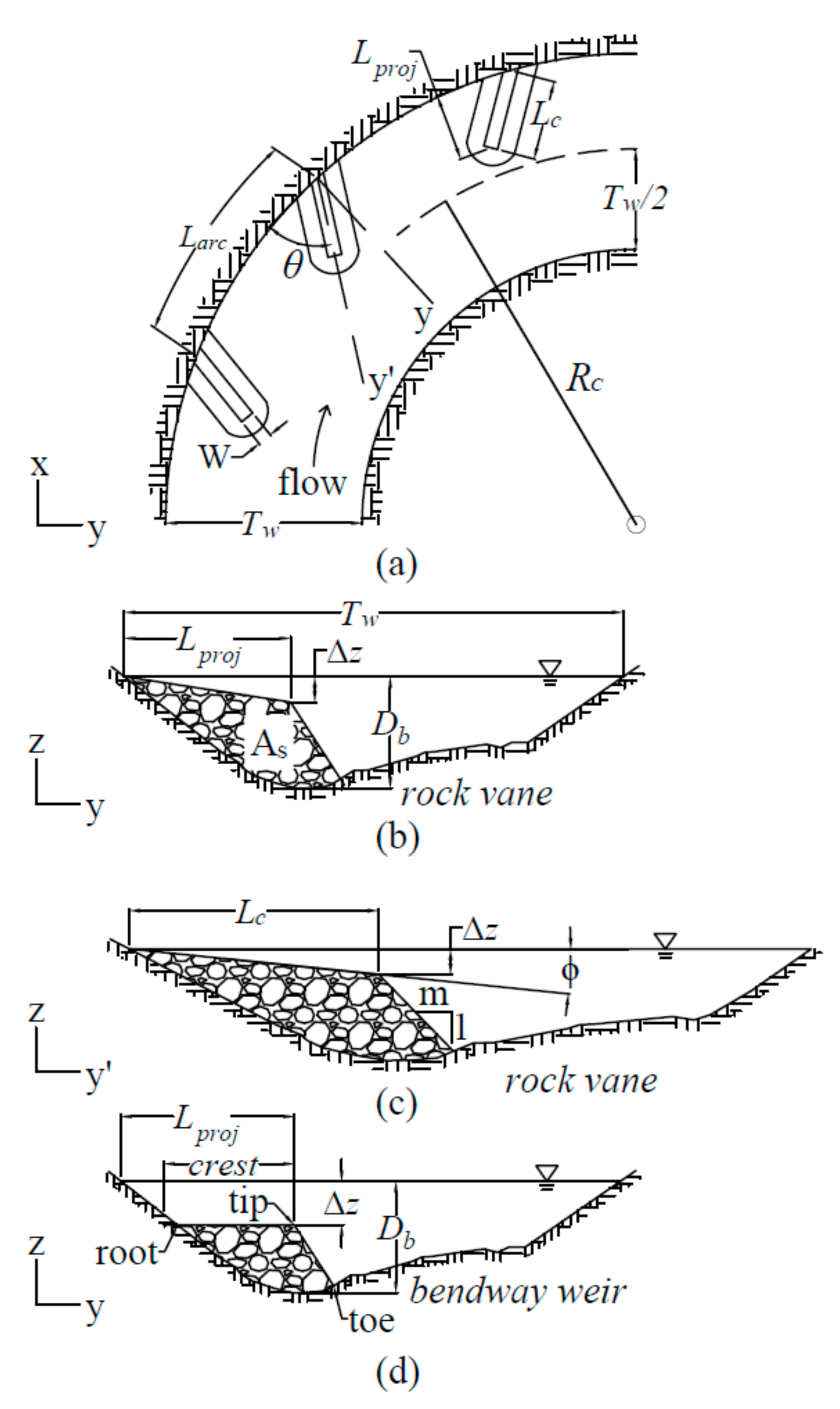
Design guides for rock vanes recommend a wide range of design values [1,2,3,4,5,6,7,8]. Recommended parameter values range from 0.10 Tw to 0.35 Tw (Tw is bankfull width, as in Figure 1) for crest length (Lc) [3]; from <20° [5] to 80° [3,4] for planform angle (θ); and from 0% [4] to 20% [5] for crest slope. The large variation in recommended values between design guides leaves the design engineer with considerable uncertainty. Bendway weir design guidelines offer similarly diverse recommendations [9,10,11]. Recommended structure crest lengths range from 0.1 Tw to 0.3 Tw [11], and the recommended crest submergence (Δz as shown in Figure 1) ranges from zero to half the main-channel depth [10].
Several physical-model, field, and numerical-model studies have investigated hydraulic performance of rock vanes and bendway weirs [12,13,14,15,16,17,18,19,20,21,22,23,24,25,26,27], and most of these studies noted the lack of comprehensive design guidance for actual field application. The geometric parameters applied in the field are specific for each case, and there is no standard approach or guidance to determine potential hydraulic performance before implementation. Physical-model and numerical-model studies, therefore, are an important resource for design engineers and offer invaluable insight into how structure designs are likely to perform in an actual field setting.
Physical model studies, while providing valuable measurements and results, are time consuming, can be expensive when major configuration alterations are needed, and sometimes do not allow rapid assessment of alternative designs based on multiple transverse feature configurations or channel configurations. Numerical modeling offers an attractive alternative, and 2D studies have been performed to study design structures [28]. 3D models, however, are also limited by computational expenses and have mainly been applied to examine only a single structure or a couple of structures [15,20]. Thus, using 2D depth-averaged models is attractive from an engineering design standpoint. Depth-averaging of the flow field does not account for the vertical velocity component in 3D flow fields generated by these structures. Therefore, identifying and quantifying deviations of the predicted flow field from the actual flow field can examine these limitations and help ascertain whether a 2D model can adequately be used to examine structure performance.
To examine the predictive capability of a 2D model of flow in a channel fitted with configurations of rock vanes or bendway weirs, we compared data from the numerical model with data from a physical model. This paper describes the physical model, which provided measurements from baseline and three rock vane and four bendway weir configurations. The numerical model results section presents results of the 2D numerical model for one rock vane and one bendway weir configuration. Lastly, information is provided on how SRH-2D can be effectively applied during the design process.
2. Materials and Methods
2.1. Physical Model Facility
A two-bend physical model that yielded extensive water-surface elevation and velocity measurements was compared with numerical-model results from the numerical model SRH-2D. The Engineering and Research Center at Colorado State University constructed the physical model at 1:12 length scale. The overall model gradient was about 0.000863 V:H. The model was constructed using cross-sectional plywood templates with steel flashing and filled with sand material. A brushed concrete surface was placed between the plywood templates. Flows were delivered from the model sump to the headbox in a recirculating system. Tailwater conditions were established to provide approximately normal flow conditions throughout the model.
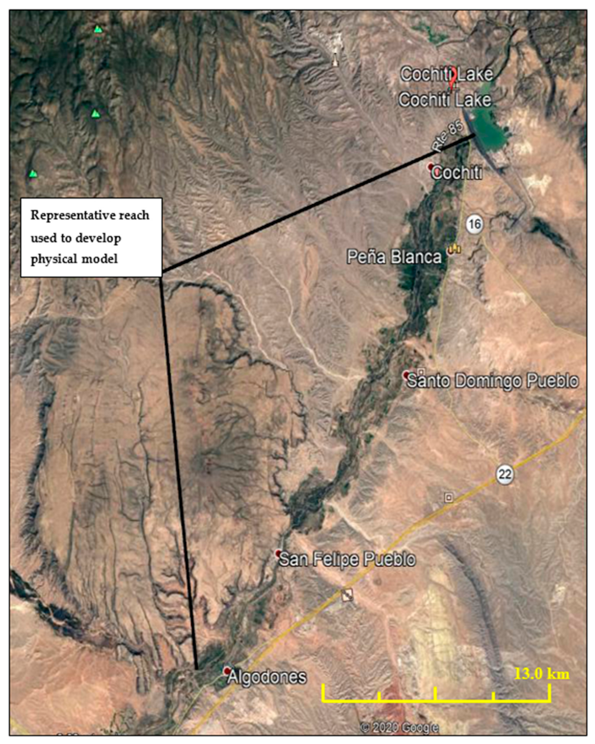
The physical model was based on a reach of the Middle Rio Grande between Cochiti Dam downstream to Angostura Diversion Dam near Algodones, New Mexico (Figure 2). In this reach, the historic low-flow, braided, sand-dominated channel had been transitioned to an incising single-thread, gravel-dominated, lateral migrating channel as a result of installation of Cochiti Dam [29]. The river’s top-width (TW) and radius of curvature (RC) were identified for channel bends in the prototype reach. In the physical model, two representative bend geometries (Figure 3) spanned the ranges of RC/TW observed from the prototype (Table 1).
The channel configurations described here represent fixed-bed native topography. Even though Cochiti bend is upstream of the San Felipe bend in the middle Rio Grande (Figure 2), the physical model switched these two to represent the natural topography in the San Felipe site as the upstream bend and the topography in the Cochiti site as the downstream bend in the physical model (Figure 4). This was done to accommodate the physical model within the laboratory configuration. The RC/TW of both bends are in Table 1.
2.2. Physical Model Transverse Feature Configurations
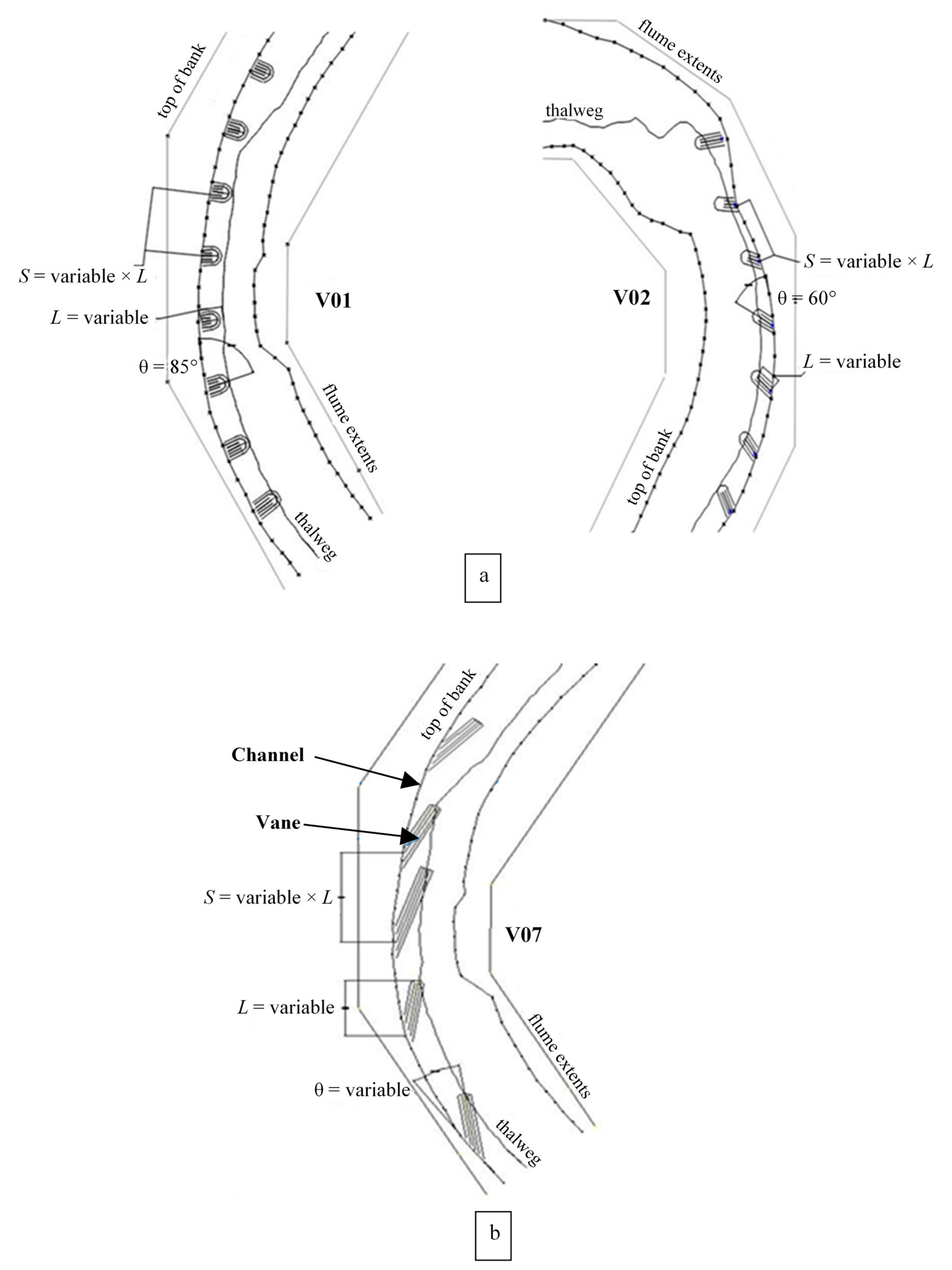
This section describes the physical model configurations with fixed bed native topography [30]. To measure and evaluate flows, [22,24,27]. We designed three rock vane and four bendway weir configurations, based upon the most common design values from the available design guidance [1,2,3,4,5,6,7,8,9,10,11]. Parameters are based on design recommendations. Table 2 provides the vane parameters and Table 3 provides the bendway weir parameters. Planimetric views of the vane design configurations (V01, V02, and V07) are presented in Figure 5 and bendway weir designs (BW01–BW04) are presented in Figure 6. Figure 7 and Figure 8 are photographs of the physical model.
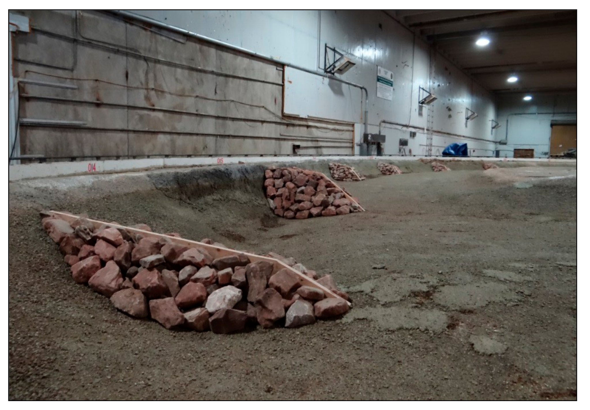
The vanes and bendway weirs were constructed using plywood to create impermeability and with tight-fitting angular stones ranging from 91 to 152 mm along the intermediate axis, in accordance with the guidelines (Table 2Table 3). Stones were sized to remain stable while testing physical models in the laboratory and for structures to be constructed according to the design recommendations in 2 and Table 3.
2.3. Physical Model Measurements
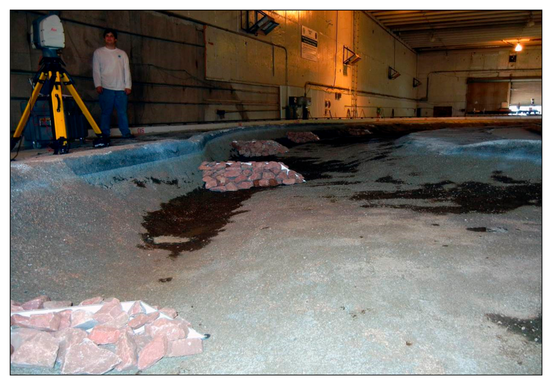
Two Acoustic Doppler Velocimeters (ADV) were used to measure velocity: a SonTek® ADV with ±1% measured accuracy, and a Nortek Vectrino® ADV with ±0.5% accuracy. Velocity was measured to the nearest 0.001 m per second (m/s), with measurement values ranging from approximately 0.003 to 1.3 m/s. The associated measurement error for these values (based on reported precisions) is negligible. For each configuration, 2500 velocity data points were measured [22,24,27]. To directly compare between laboratory configurations and between laboratory and numerical model results, measurements were made at consistent locations for baseline, rock vanes, and bendway weirs. To measure depth-averaged velocity (approximated as the velocity at 0.6 of the flow depth below the water surface), these data points were along the thalweg, along seven cross-sections, placed in a more dense grid around one structure in each bend for each test, and placed throughout the physical model (Table 4 and Figure 9).
The water-surface elevation for each configuration was measured at the bankline at approximately 0.15 m intervals using a Leica Total Station laser-surveying unit with a 3D point accuracy of 0.2 mm. Bed topography was measured with a Leica ScanStation 2® (Leica Geosystems AG, Heerbrugg, Switzerland), a terrestrial light detection and ranging unit (LiDAR) with 6-mm position accuracy, 4-mm distance accuracy, and 2-mm modeled surface precision.
2.4. SRH-2D Numerical Model
For this study, we used the SRH-2D (v 3.0) model [31], a two-dimensional (2D) depth-averaged numerical model specifically designed for river-flow hydraulics. SRH-2D adopts a zonal approach for coupled modeling of channels and floodplains. In this approach, a river system is broken down into modeling zones (delineated based on natural features such as topography, vegetation and bed roughness), each with unique parameters including flow resistance, which is specified in a Manning’s roughness coefficient. SRH-2D uses an unstructured hybrid mixed element mesh that is based on the arbitrarily shaped element method [32] for geometric representation. This meshing strategy is flexible enough to model zones, enables greater modeling detail in areas of interest—and ultimately leads to increased modeling efficiency by balancing solution accuracy and computing demands.
2.4.1. Model Setup and Calibration
We used SRH-2D to compute channel hydraulics in the fixed-bed mode. Inputs included the physical model’s topographies, discharge at the upstream boundary, and the measured downstream water surface elevation. We used the Surface-water Modeling System (SMS) software (v 13.1) [33] to generate a 2D mesh of quadrilateral elements in the main channel, to delineate model roughness areas and to assign the model boundary conditions. The pre-processed mesh as well as the roughness and boundary variables served as inputs to the SRH-2D solver.
The SRH-2D model was calibrated for baseline configuration (corresponding with the physical model’s baseline configuration), one dataset for a rock vane configuration and one dataset for the bendway weir configuration. During the calibration, we adjusted the bed roughness values iteratively, and we compared the predicted flow fields with the measured flow fields using water-surface elevations and depth-average resultant velocities.
To calibrate the baseline condition, we applied a discharge rate of 0.34 cubic meters per second (m3/s) at the upstream boundary in the physical model. However, as the physical model operations had a small but unquantified amount of seepage, we needed to adjust the upstream boundary inflow rate and bed roughness in SRH-2D as part of the calibration process. We compared SRH-2D computed velocity results with lab-measured depth-averaged velocities and calculated the corresponding Root Mean Square Error (RMSE), Mean Absolute Error (MAE) and the Mean Absolute Percentage Error (MAPE). For this calibration, “error” is defined as the difference between computed and measured fields. Based on the RMS and MAE results, a discharge value of 0.325 m3/s (seepage of 0.015 m3/s) and a Manning’s roughness coefficient of 0.018 were determined to be the values that best matched the measured data (Table 5). We used the velocity field for the RMSE, MAE, and MAPE analyses rather than the water-surface elevation (WSE) as velocity field had a larger variance in the velocity distribution than the WSEs did. This larger variance, which can be readily seen in the “filled” contour plots presented in the results section, made velocity a better discriminator of model performance between the configurations examined. Moreover, velocity is a more important parameter than water-surface elevation when evaluating the efficacy of a transverse feature design.
The mesh resolution used in a 2D model can influence the model’s results if not selected carefully. Before the roughness calibration, we tested three mesh sizes to establish grid independence (i.e., the most computationally efficient mesh where smaller cell sizes did not change the results significantly) (Table 6 and Figure 10). The results are shown in Figure 11. While the three mesh sizes did not appreciably affect velocity results, the coarse mesh size did not adequately resolve the flow separation zones associated with the upstream bend contraction (Figure 11). The medium-sized mesh (Figure 10) was therefore selected for all the model runs.
After establishing grid independence and calibrating the roughness under the baseline configuration, the next step was calibrating SRH-2D against model measurements with structures in place. Because the LIDAR had a high accuracy rating, the surface topography of the rock structures had enough accuracy for the numerical model. Because the physical model replications of rock vanes and bendway weirs used angular rock approximately 91 to 152 millimeters (mm), at least 15 to 25 LiDAR data points were measured over the diameter for each angular rock—providing good representation of the rock structure roughness with the topography. The medium mesh cell sizes adequately captured rock forms as the cells were generally smaller than the rock diameter. Manning’s roughness values representing skin friction were successively changed (n = 0.018–0.05) over the footprint of transverse features. Setting the structure roughness at the same value of the baseline calibrated n = 0.018 produced an ideal match to measured depth-averaged velocity. Scurlock et al. [34] also found that setting the physical model structure’s roughness value equal to the numerical model’s baseline roughness value resulted in the most ideal measured velocity match for models using FLOW 3D, Flow Science®’s 3D numerical model.
2.4.2. Velocity Zone Comparison
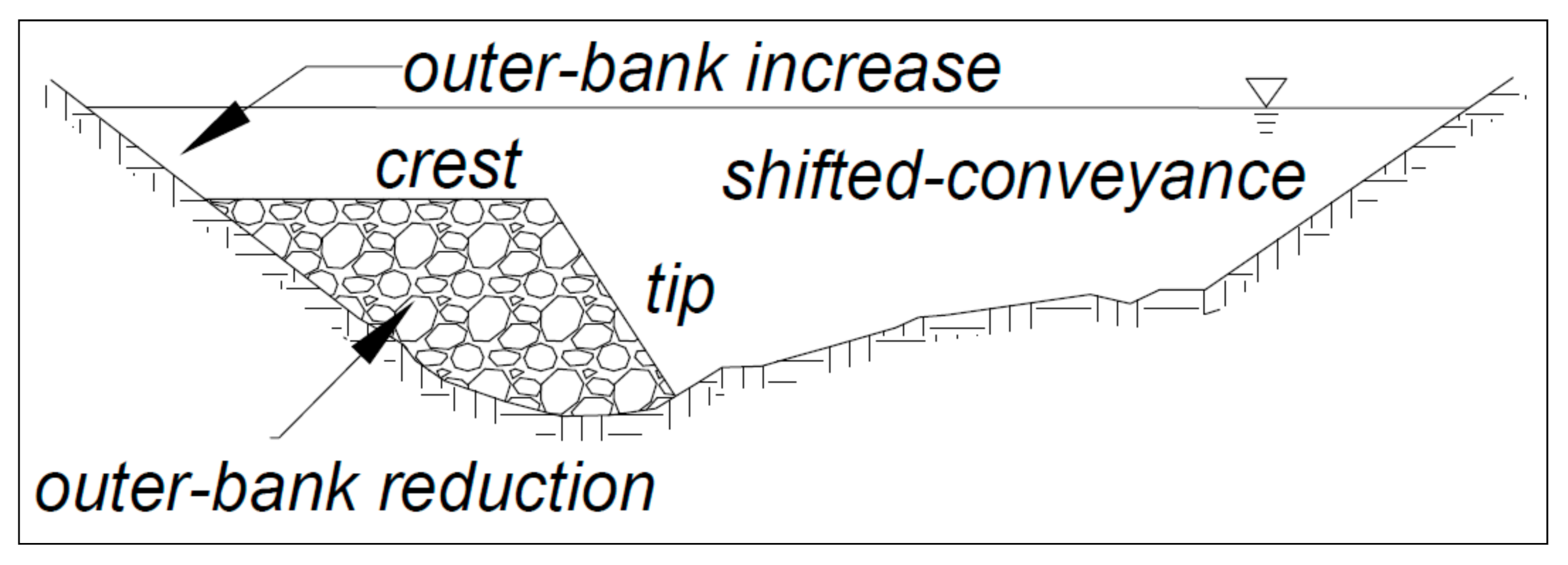
Flow field comparisons between the physical model and the numeric model are categorized by the distinct characteristic flow zones that define rock vane and bendway weir hydraulics. These separate regions of identifiable velocity trends from rock vane and bendway weir structures (described in Figure 12 and Table 7) have also been noted by [12,13,15,23]. These regions include: the outer-bank reduction zone, the shifted-conveyance zone at the center of the channel and inner-bank, the outer-bank increased zone, and zones of convective acceleration at the structure crest and tip. Although vanes slope from the top of bank (crest zone) down to the bed at the free end (tip) they have essentially the same flow zones as bendway weir (Figure 12).
3. Results
3.1. Depth-Averaged Velocity Verification
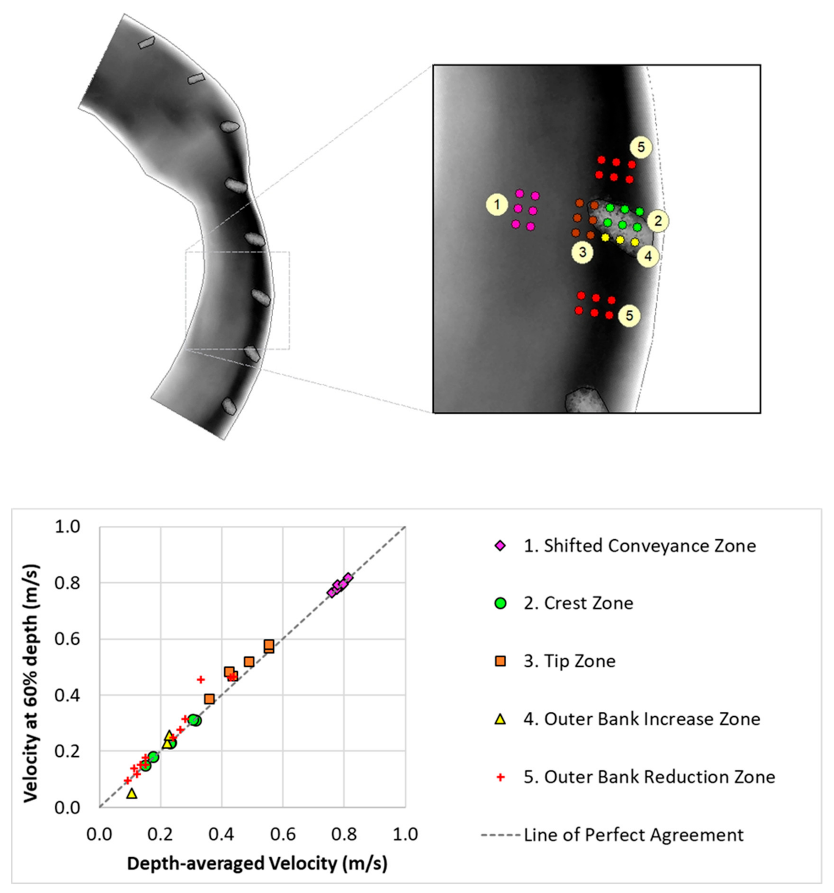
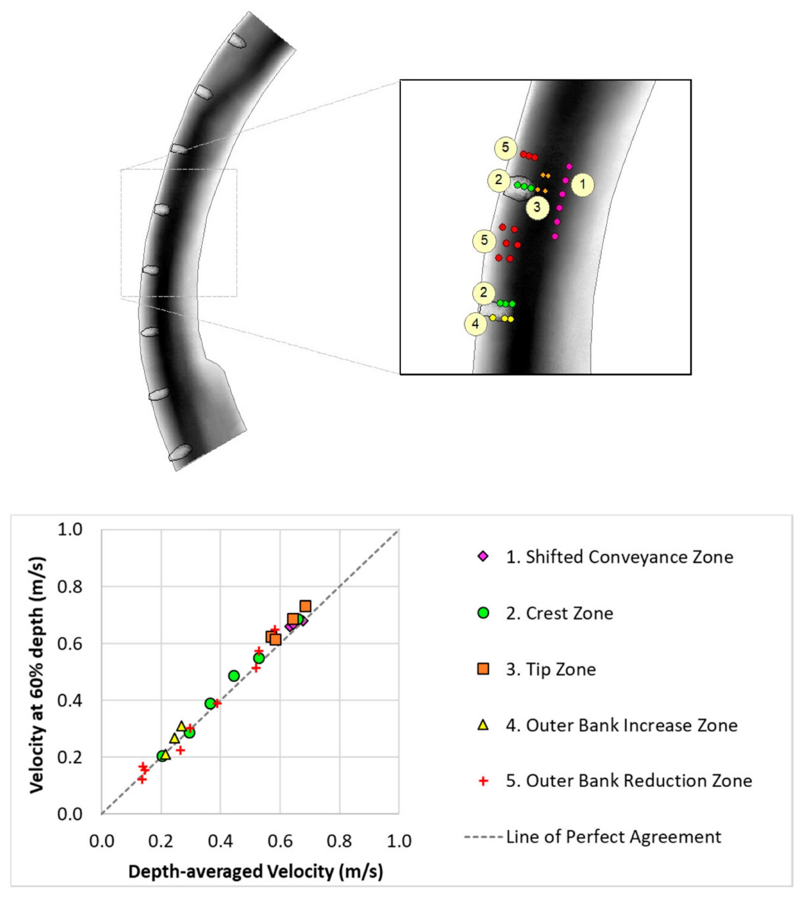
The physical modeling took measurements at the same flow locations for the baseline, rock vanes and bendway weirs as described in Section 2. To approximate depth-averaged velocities, we took these measurements at 60% of the flow depth from the water surface (Table 4 and Figure 9). To determine if the 60% depth measurements were appropriate to directly compare with SRH-2D output and to measure the flow field, we measured a denser grid at 5% depth intervals around one structure in each rock vane and bendway weir configuration, and measured 20% depth intervals along the outer bank. To compare the depth-averaged velocity at each of these measurement locations with the 60% depth measurements, we integrated the 5% and 20% depth interval data over the depth using the trapezoidal rule. Overall, the integrated velocities from the 5% and 20% depth compared well with the velocities measured at 60% of the flow depth (Figure 13 and Figure 14). This result indicates that the 60% depth velocity measurements are a good approximation of the depth-averaged velocity.
3.2. Baseline Configuration: Physical and SRH-2D Numerical Model Comparisons
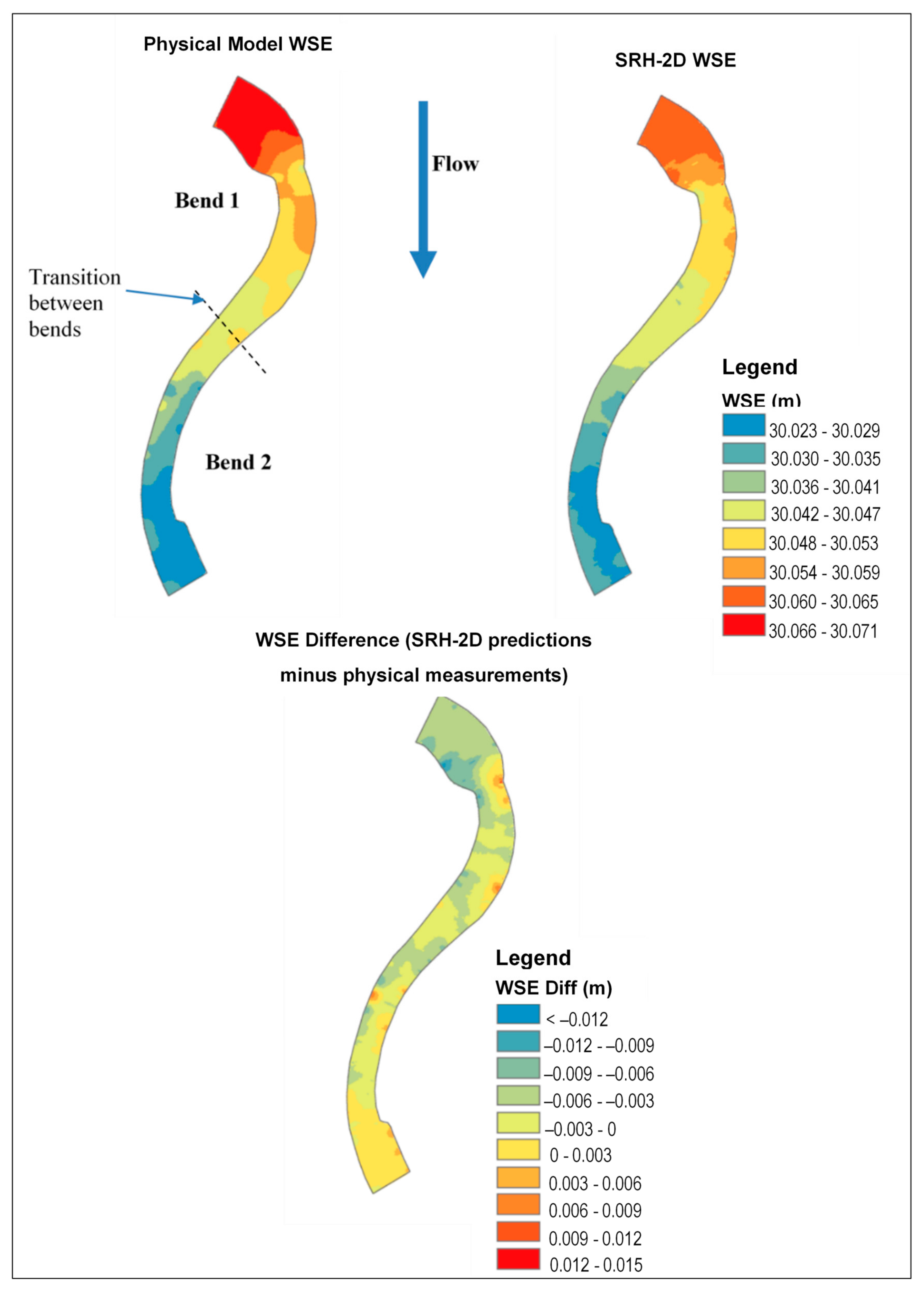
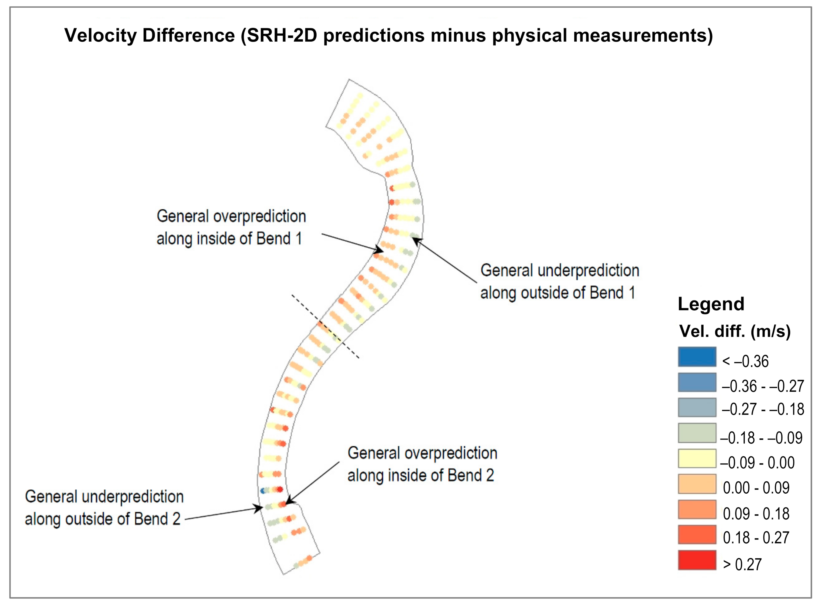
Figure 15 shows the physical model’s measured and SRH-2D model’s predicted water-surface elevation (WSE), and Figure 16 shows the velocity fields for the upstream bend (Bend 1) and the downstream bend (Bend 2). In each of these figures, the colored shading indicates the contours, which were derived from the data using inverse distance weighting to create a Raster surface. The “difference” plot derived by subtracting the physical model’s measured WSEs from the SRH-2D-predicted WSEs is also shown in Figure 15. Because there are larger variations in the velocity field, the “difference” plot for velocity is shown in a separate figure (Figure 17). To avoid distortions introduced by interpolation, only results at the measurement locations are shown in Figure 17.
Overall, the WSEs from the physical and numerical model results show good agreement, with a slight underprediction in Bend 1 (predicted values are generally 0 to 0.006 meters (m) lower than the measured values) and a slight overprediction in Bend 2 (predicted values are generally 0 to 0.006 m higher than the measured values). The differences between the measured and predicted velocity contours are more pronounced than the differences in WSE. The remainder of this section, therefore, focuses on comparing the measured and predicted velocity contours.
At the upstream section of the physical model, velocity is highest in the area on the inside of Bend 1 (Figure 16). The high-velocity zone extends through and immediately downstream of the contraction, with the highest velocity occurring on the outside of the bend. Upstream of the contraction, velocity is lower as the channel experiences a backwater that develops the head for the flow to pass through the contraction with associated energy losses. Downstream of the contraction, the next-highest velocity area is along the outside of the Bend 1, starting from just upstream of the bend apex and stretching through the downstream side of the bend. Through the crossing (i.e., transition between Bend 1 and Bend 2), the high-velocity zone is along the left bank until the zone reaches the inside of Bend 2. Through the bendway, the zone of high velocity crosses over the channel, such that the high velocity reaches the outside bank of Bend 2 near the bend apex. The high-velocity zone stays along the outside bank through to the physical model exit.
SRH-2D model results for the baseline configuration (Figure 16) also show a higher velocity area on the inside of Bend 1 in the upstream section. There is a high-velocity area at the contraction, with the highest velocity near the inside of the bend, which appears to be due to the contraction effect rather than entrance conditions. Throughout Bend 1, the high-velocity area is nearly symmetrical with a smaller higher-velocity area near the outer bank on the downstream of the bend. A small skew in the high-velocity area towards the outer bank at the downstream boundary of Bend 1 remains on the left bank as the flow transitions into Bend 2. As the flow enters Bend 2, high-velocity flows are on the inside of Bend 2. Downstream of the transition, the high-velocity area becomes more symmetrical within the channel width, with a slight skew towards the outer bank and high-velocity flows remain in this alignment until the downstream model boundary. The highest-velocity area is just downstream of the Bend 2 apex and extends for a short distance.
The velocity differences are compared in Figure 16.
SRH-2D overpredicts flow velocities on the:
- inside Bend 1,
- upper half of the outside of Bend 2,
- inside of the Bend 2 near the end of the physical model.
The overprediction is mostly about 0 to 0.09 m/s with a few areas of 0.09 to 0.18 m/s. Overpredictions are also within 20% of the measured velocities, while most differences are much less. These differences are relatively small, and it may be concluded that there is good correspondence between the measured and predicted through both bends.
There is general agreement between the SRH-2D WSE and velocity predictions and the measurements.
SRH-2D underpredicts the velocity:
- along the outside of Bend 1,
- through the upper portion of the inside of Bend 2,
- on the outside of the downstream portion of Bend 2.
However, the difference magnitude is relatively small—mostly about −0.09 to 0 m/s with a few locations about −0.18 to −0.09 m/s. SRH-2D velocity predictions are within 20% of the measured velocities, and most areas are even closer.
3.3. Rock Vane Configuration: Physical and SRH-2D Numerical Model Comparisons
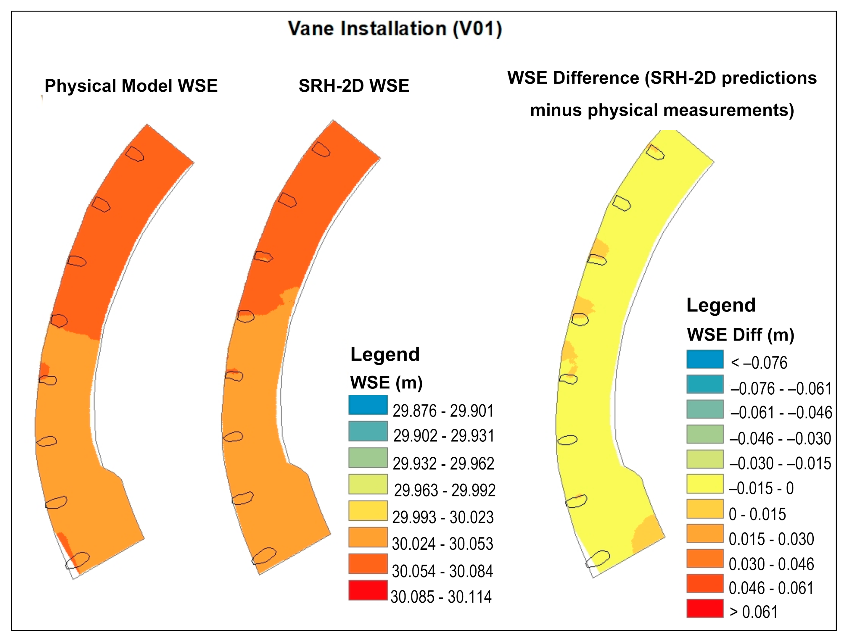
This section presents results for the rock vane configuration V01 installation WSE (Figure 18) and depth-average velocity (Figure 19). Like the baseline configuration, the measured WSEs compared well with the predicted elevations, with most of the differences from −0.015 to 0 m, and some small areas with differences between 0 and 0.015 m, and the rest of this section, therefore, focuses on velocity.
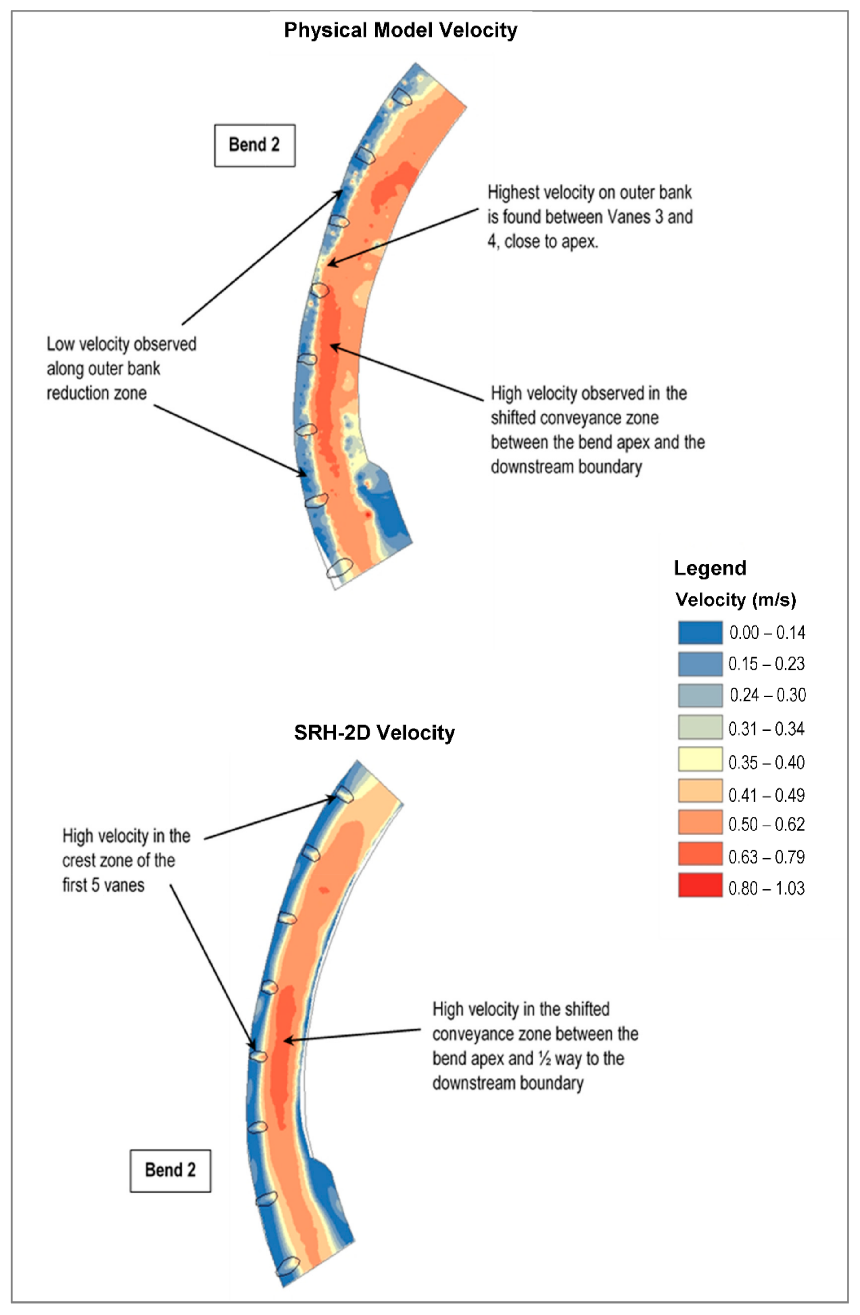
Physical model measurements show that the highest velocity area (0.63 to 0.79 m/s) is in the shifted conveyance zone between the bend apex and near the downstream model boundary. The remainder of the shifted conveyance zone is a high-velocity area, with magnitudes ranging from 0.50 to 0.62 m/s. There is also high velocity in the crest and tip zones for the first five vanes. The vanes induce low-velocity (0.15 to 0.23 m/s) banklines out to near the tips of the vanes, in the outer bank reduction zone. The highest velocity region is in the shifted conveyance zone from about the bend apex downstream to near the second-to-last vane.
SRH-2D-predicted velocity patterns are close to the physical model’s measured flow patterns. The outer bank reduction zone is well defined from the bank to near the vane tips, with low flow velocities ranging from 0 to 0.23 m/s. The high velocity in the shifted conveyance zone has similar flow regions and velocity ranges in the physical model’s measurements and the SRH-2D predictions. The SRH-2D-predicted highest velocity is in the same location as the physical model’s measured highest velocity in the streamwise direction, but the predicted velocity area is farther away from the vane tips in the transverse direction than the physical model’s measured area.
The velocity differences are compared in (Figure 20).
SRH-2D overpredicts velocities in the:
- crest zone;
- out bank increase zone downstream of the first three upstream vanes;
- fifth vane (in the fifth vane by 0.09 to 0.18 m/s);
- sixth vane (in the sixth vane by 0 to 0.09 m/s);
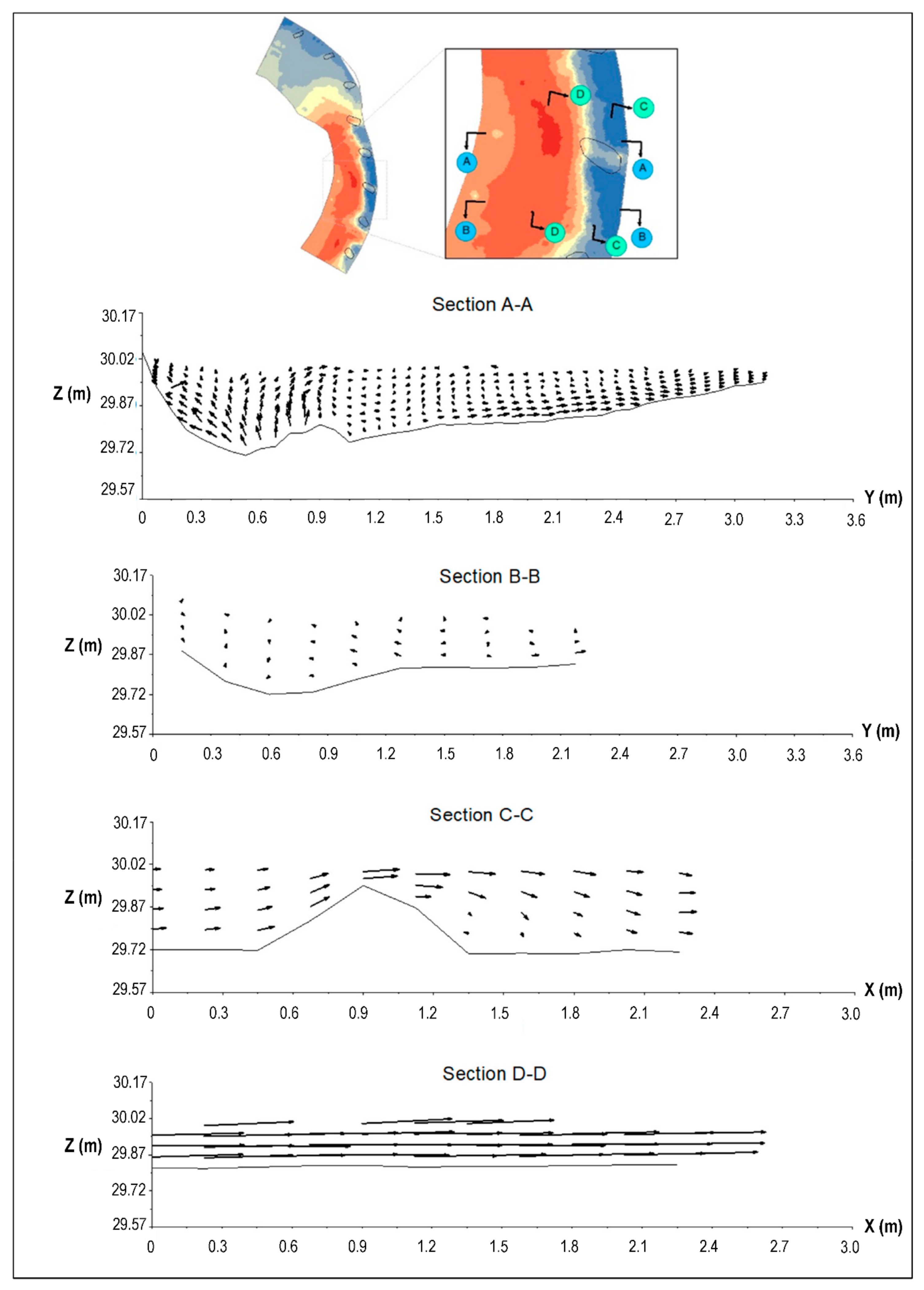
- tip and shifted conveyance zones where flow has a significant vertical velocity component (Sections A-A and B-B in Figure 21);
- areas where flow vertically contracts and expands (outer bank increase zone) over the structures (Section C-C Figure 21);
- tip zone where there is vortex shedding and associated turbulence kinetic energy (Section A-A Figure 21).
SRH-2D generally underpredicts flow velocities in the:
- shifted conveyance zone throughout the bendway (−0.18 to 0 m/s);
- tip zone of Vanes 4, 6, 7, and 8 (−0.18 to −0.09 m/s);
- localized zones along the outer bank around Vanes 4, 6, 7, and 8 (−0.18 to −0.09 m/s);
- areas where the shifted conveyance zone is not fully captured.
3.4. Bendway Weir Scenario Configuration: Physical and SRH-2D Numerical Model Comparisons
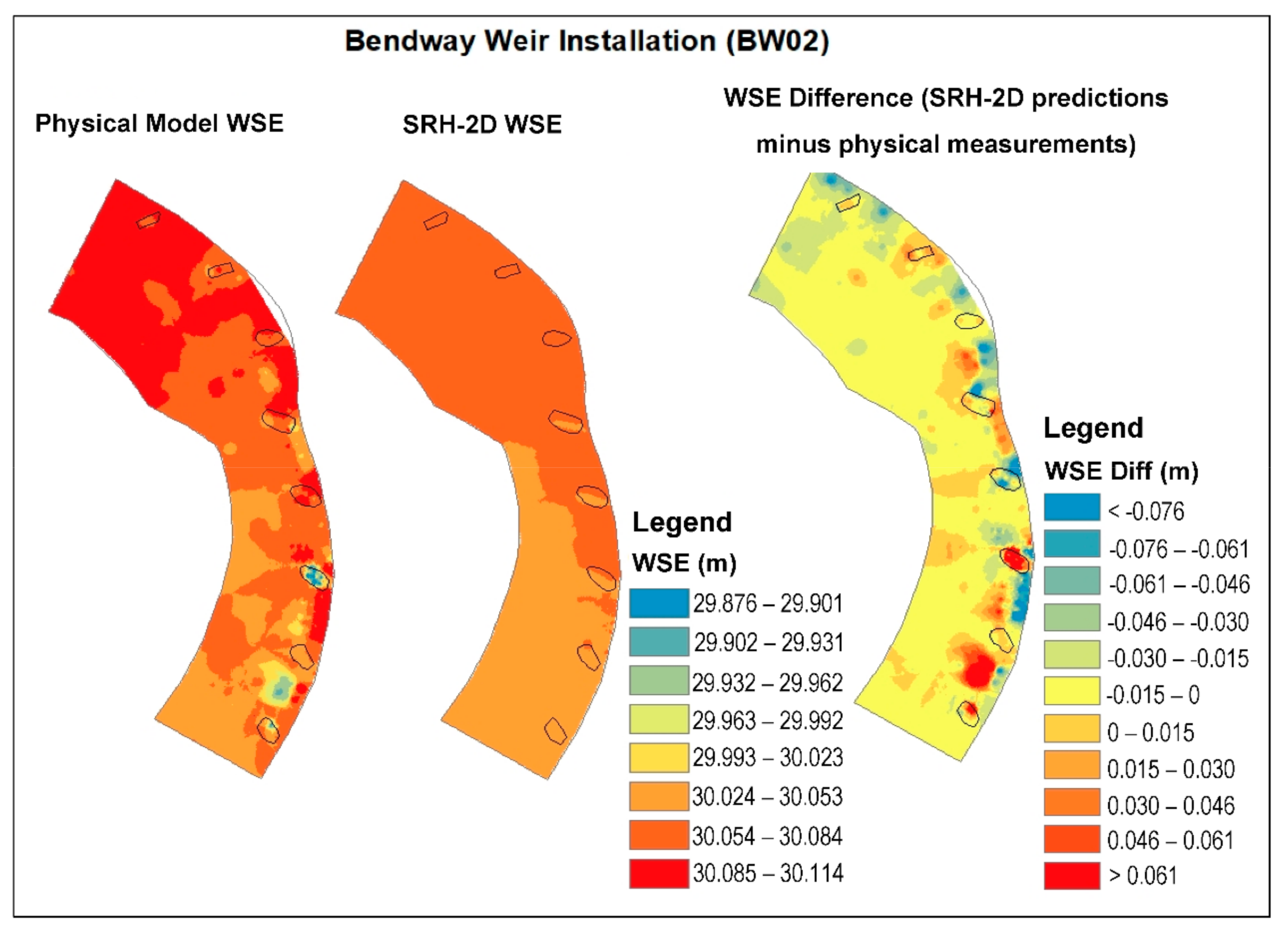
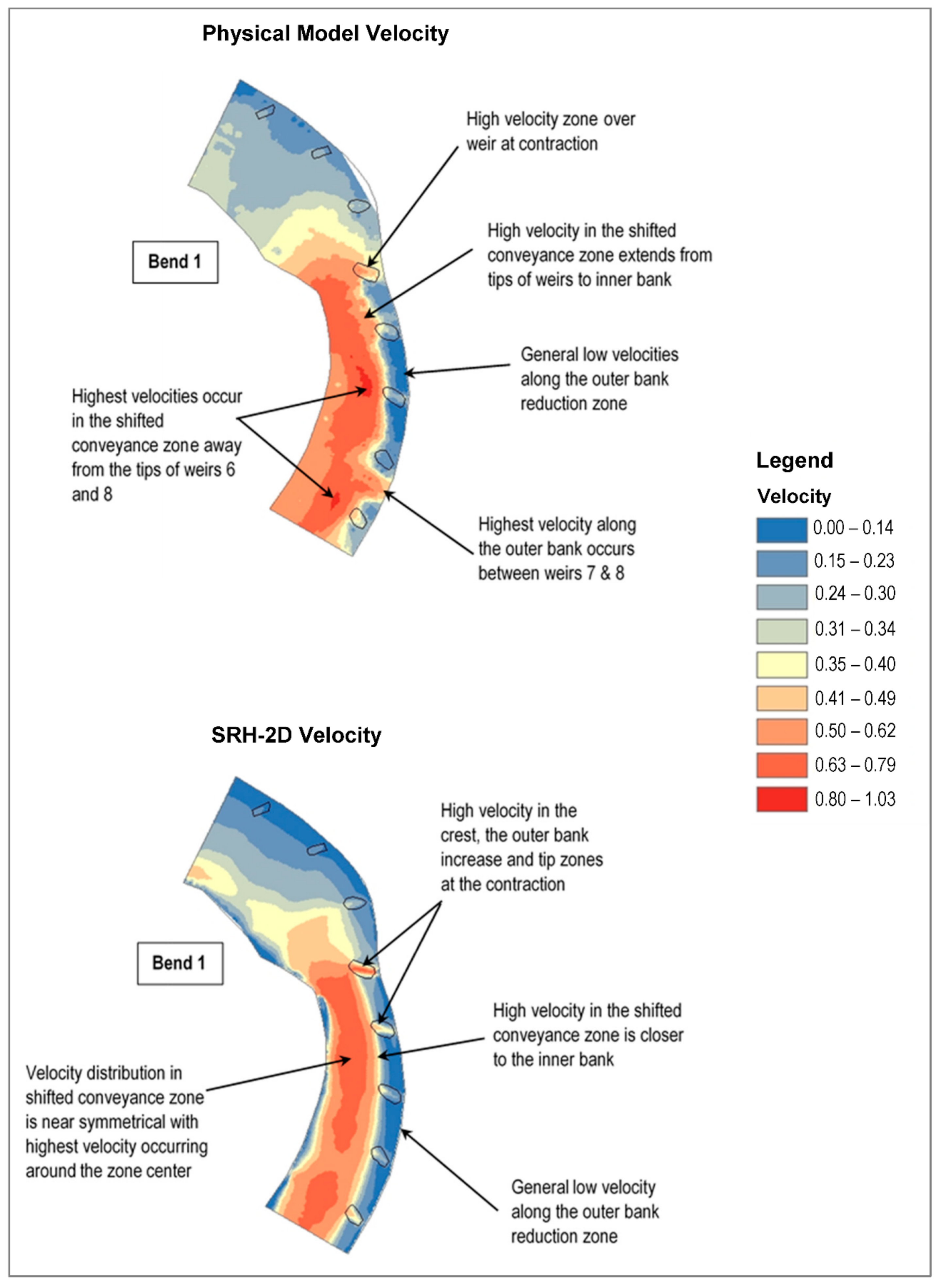
This section presents results for bendway weir configuration BW02 WSE (Figure 22) and velocity (Figure 23 and Figure 24).
Physical model measurements show a high-velocity zone that moves away from the outside of Bend 1 in the outer bank reduction zone, in contrast to the baseline configuration without the structures, where the high velocity was along the outer bank. The high velocity shifts away from the weirs toward the inner bank in the shifted conveyance zone. There is, however, a local high-velocity area between Bendway Weirs 7 and 8 within the outer bank reduction zone, but it does not extend to the bankline [23]. This local area could be from the interactions between flow eddies and the structures. Within the shifted conveyance zone, local pockets of highest velocities are seen close to the tips of Bendway Weirs 6 and 8. Upstream, at the contraction, there is high flow acceleration over the first bendway weir that is not observed over the other weirs. This high flow acceleration of the first bendway weir is also predicted by SRH-2D—suggesting that it is driven largely by the contraction effects.
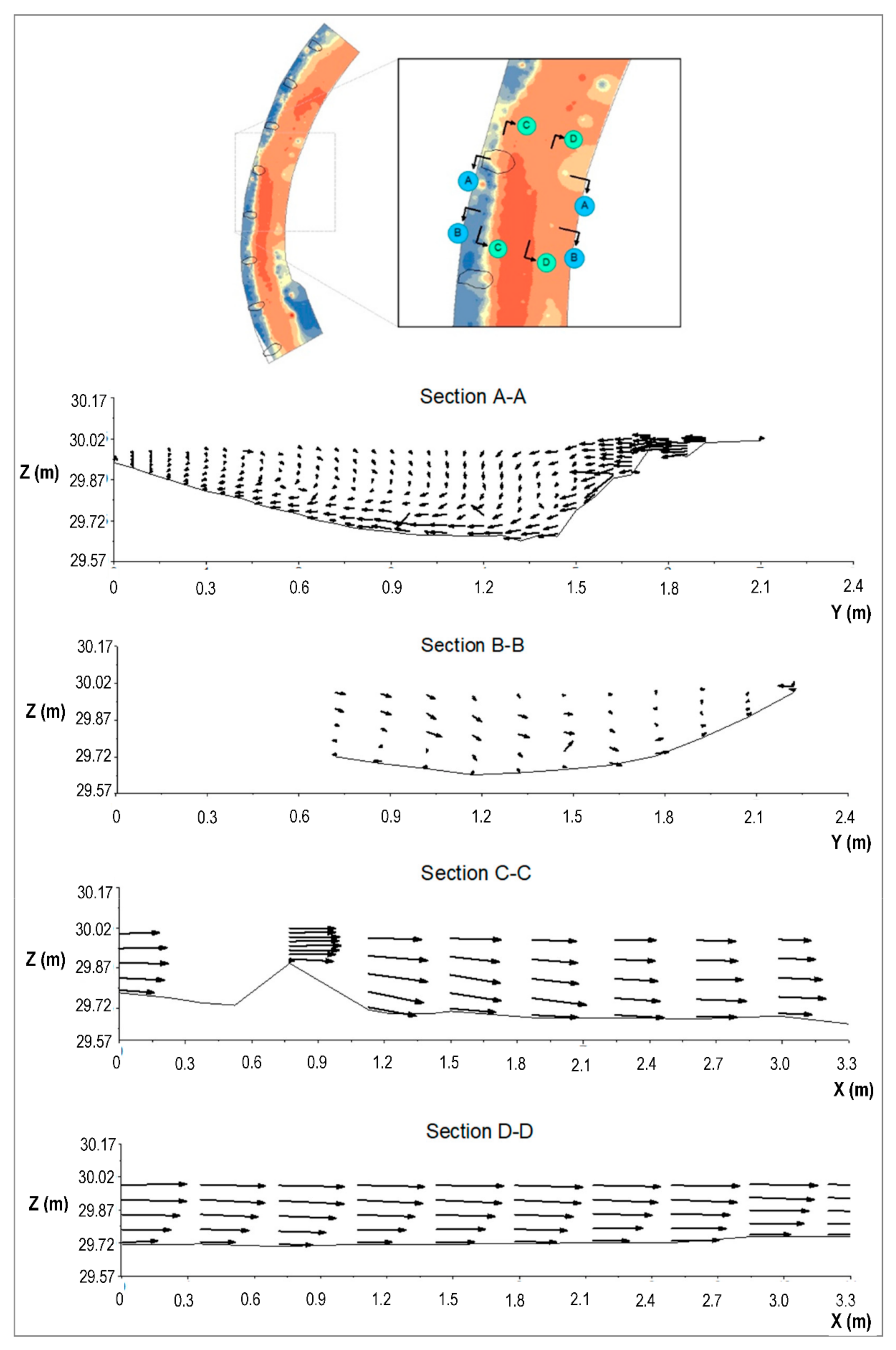
SRH-2D was able to predict the shift in high velocity away from the outer bank reduction zone. The highest-velocity zone was, however, a little farther away from the weir tips than the measured zone in the physical model. SRH-2D did not predict the local high-velocity zone between Bendway Weirs 7 and 8—suggesting that the presence of the zone in the physical model likely caused flow features with significant vertical velocity components (Figure 25). In design, underprediction along the bankline could lead to a failure to recognize the potential for accelerated bank erosion that could flank Bendway Weir 8. Approaches to provide a stable design configuration are included in Section 4.3. Overall, SRH-2D predicted regions of both higher and lower velocities in the shifted conveyance zones as well as between the weirs. Velocity vectors illustrate the high velocity along the crest zone of the bendway weirs (Sections A-A and C-C Figure 25). The velocity downstream of the bendway weir near the bankline (Section C-C in Figure 25) is nearly as great as the velocity in the shifted conveyance zone (Section D-D in Figure 25).
The WSEs at Bendway Weir 6 (counted from bend entrance) and an area between Bendway Weirs 7 and 8 were overpredicted by SRH-2D. However, the measured WSE is about 0.15 m lower than nearby measurements—suggesting these locations were inaccurately measured.
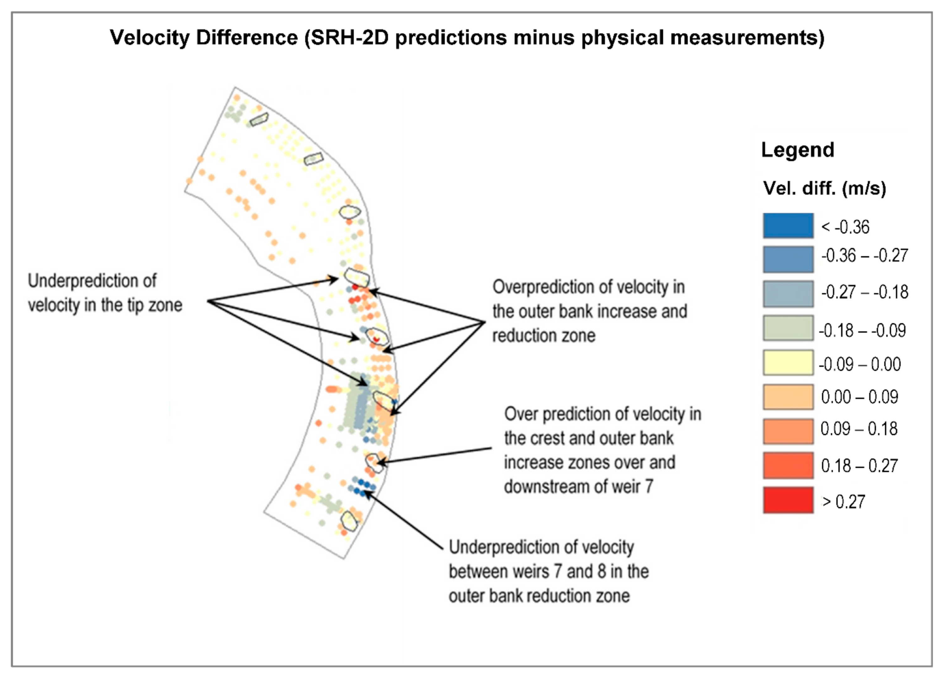
SRH-2D consistently overpredicts velocity:
- over the bendway weir crests;
- downstream of each weir;
- downstream of the weir tips (weir tips by about 0 to 0.18 m/s).
Interestingly, the velocity is underpredicted:
- at the tips of Weirs 6 and 8;
- between Weirs 7 and 8 along the bank (Weirs 7 and 8 by −0.36 to −0.27 m/s).
The lower velocities in the center of the channel near Bendway Weirs 7 and 8 and along the bank between the bendway weirs may be a result of SRH-2D’s failure to capture conveyance shifts from changes in the flow field caused by flow-structure interactions.
SRH-2D underpredicted the WSE by about −0.015 to 0 m throughout most of Bend 1. The underprediction was larger in areas along the outside bank (−0.076 to −0.061 m). In a few selected areas, SRH-2D underpredicted the WSEs by about −0.03 to −0.015 m.
4. Discussion, Summary and Conclusions
4.1. SRH-2D Model Performance
A summary of velocity results for the baseline, rock vane and bendway weir configurations is presented in Table 8. Velocity zones, defined by distinct hydraulic conditions (Figure 12 and Table 7), are identified where differences occur between computed and measured velocities.
Measured and predicted results from SRH-2D have the same general velocity patterns, indicating that SRH-2D can be used for design applications with a factor of safety as described in Section 4.3. SRH-2D overpredicts velocity in the crest zone, tip zone and sometimes in the shifted conveyance zone—generally where there is a vertical velocity component and turbulent kinetic energy. These increases are often on the order of 0 to 0.09 m/s and occasionally as high as 0.18 m/s. SRH-2D also shows both over- and underpredictions compared to measurements in zones where it cannot adequately resolve flow conveyance shifts due to the neglect of vertical-velocity components. In these zones, the increased and decreased velocities are necessary for mass conservation. Nonetheless, the predicted velocities are within ±25% of the measured velocities, with some localized exceptions. The difference is much less in most locations, which suggests good agreement between the measured and predicted results. In the shifted conveyance zone (Section D-D in Figure 21 and Figure 25), the velocity vectors are nearly uniform.
The structures induce secondary currents in the opposite direction of typical bend flow in the shifted conveyance zone (Section A-A in Figure 21 and Figure 25). In general, however, the longitudinal velocity magnitude is much greater than the lateral or vertical velocity components. This higher longitudinal velocity is the underlying reason for the velocity measured at 60% of the depth below the water surface matching the integrated/computed depth average velocity (Figure 13 and Figure 14).
Papanicolaou et al. [28] compared the FESWMS 2D model with a physical model. They reported differences of up to 60% between measured and predicted flow velocity using a single set of model input (i.e., the same Manning’s n and eddy viscosity) for the whole domain. When Papanicolaou et al. [28] changed the model input variables for each flow zone, the model performance improved, predicting differences comparable to those noted in this study (i.e., velocity differences up to 25%). SRH-2D was able to reach an accuracy of within ±25% using a single Manning’s n input value for the whole domain, which is easier for design application.
4.2. Modeling Summary
Transverse features or indirect bank-stabilization methods such as rock vanes and bendway weirs, based on experience or anecdotal design assumptions, have been used for many decades. We examined the ability of a two-dimensional depth-averaged model to predict the flow field around these structures in a two-bend 1:12-scale physical model developed from two Middle Rio Grande river bends. These bends represent conditions downstream of Cochiti Dam where the river channel has transitioned from a wide, shifting sand substrate and low-flow braided condition to a gravel-dominated bed, single thread, slightly sinuous channel.
We measured depth and velocity in the native topography simulated in the physical model without the rock structures (baseline) and then in three rock vane configurations and four bendway weir configurations. The measured data comprised about 2500 velocity measurements within the physical model at the design flow of 0.34 m3/s. LiDAR topography was measured for baseline and each configuration.
The physical model was not impervious and leaked. Leakage was not measured but was determined by evaluating combinations of reduced flow rates and Manning’s roughness coefficient. This calibration resulted in selection of water flowrate = 0.325 m3/s and Manning’s n = 0.018.
The depth-averaged SRH-2D developed by [31] used the adjusted model inflow and calibrated roughness together with each set of LiDAR (converted to a surface) and a computational mesh to evaluate each physical model configuration.
4.3. Design Implications of Model Results
The good correspondence between the SRH-2D predictions and the physical model measurements suggests that SRH-2D can be a useful tool for modeling hydrodynamics of rock vanes and bendway weirs for design. Key SRH-2D model observations derived from evaluating all the model runs for the configurations in Table 2 and Table 3—and how they may influence design—are:
- SRH-2D model results matched the overall flow patterns found in physical model measurements for rock vanes and bendway weirs. Thus, SRH-2D models can be used to compare the effects of spacing, length, horizontal angle (rock vanes) and orientation angle of different structure configurations.
- SRH-2D did not compute the high-velocity zone between Bendway Weirs 7 and 8 (Figure 25). Higher velocities exist on the downstream portion of river bends (Figure 16). Additional bank erosion countermeasures such as bioengineering [35] could be employed between bendway weirs located in the downstream section of river bends, as well as between other weirs.
- SRH-2D computes increased resultant velocity when compared to physical model measurements over transverse feature crests and right at the tips where there is a vertical-velocity component and turbulent kinetic energy. Overprediction varies between approximately 15 and 25%, with a few locations over this range. This overprediction provides conservative design. And we recommend that model results be used over weir crests when designing erosion countermeasures such as bioengineering [35].
- SRH-2D may not fully resolve conveyance shifts. This failure to fully resolve can lead to both overprediction and underprediction of velocity in certain zones of the flow field by up to 25%, depending on the configuration. The highest velocity found in the shifted conveyance zone or at the tip is conservative and should be used for design tip scour and riprap sizing. Transverse feature rock sizing procedures from large-scale flume experiments [36] should be used, along with an appropriate factor of safety [37]. These higher velocities might affect sediment transport analysis, but this study did not determine the magnitude of this effect.
- SRH-2D underpredicts bankline velocity in some locations by up to about 25%. Increase bankline velocity by at least this amount during design.
4.4. Conclusions
The velocity differences between SRH-2D predictions and physical-model measurements are more pronounced (Figure 17, Figure 20 and Figure 24) than WSE differences (Figure 15, Figure 18 and Figure 22). Results show a useful agreement between SRH-2D estimates and the measurements. Therefore, SRH-2D is a suitable tool to compare combinations of transverse feature length, spacing, horizontal and vertical angles (rock vanes), and crest elevation (bendway weirs). SRH-2D generally predicted increased velocity (between 15 and 25%) in flow regions with a vertical velocity component and turbulence kinetic energy (tip and crest zones). These numerical model predictions are suitable for conservative designs. There also were local regions where SRH-2D underpredicted the velocity (up to 25%) at the outer bank zone and at the tip zone of select features. Increasing bankline velocity for design up to 25% is recommended. The crest extending from the top of bank and sloping down to past the thalweg in rock vanes allows rock vanes to provide much better bank-line velocity reduction than bendway weirs. As such, bendway weirs are not recommended for bank protection—and should only be used for thalweg management unless additional erosion countermeasures are also employed.
Author Contributions
Conceptualization, D.C.B., S.M.S., S.B.A. and C.I.T.; methodology, D.C.B., B.A. and S.M.S.; numerical modeling, B.A., D.C.B.; validation, D.C.B., B.A.; formal analysis, B.A., D.C.B.; investigation, S.M.S., S.B.A., C.I.T. and D.C.B.; writing—original draft preparation, D.C.B., B.A.; writing—review and editing, D.C.B., B.A., S.M.S., S.B.A. and C.I.T.; supervision, D.C.B., C.I.T.; project administration, S.B.A., C.I.T. All authors have read and agreed to the published version of the manuscript.
Funding
Colorado State University received funding from the Bureau of Reclamation under agreement number R14AC00045.
Institutional Review Board Statement
Not applicable.
Informed Consent Statement
Not applicable.
Data Availability Statement
The data presented in this study are available on request from the corresponding author. The data are not publicly available due to not having a web site available for public access.
Acknowledgments
Robert Ettema reviewed a draft of the paper and offering helpful comments. Nathan Holste, Robert Padilla and Ari Posner provided review and helpful suggestions during this work.
Conflicts of Interest
The authors declare no conflict of interest. The funders had a limited role in the design of the study. The funders had no role in the collection, analyses or interpretation of data, or in the writing of the manuscript. The funders had a limited role in the review of the study results and in the decision to publish the results. The findings in this paper are technical in nature and have been determined by the authors, and are not official policy of the Bureau of Reclamation.
References
- Washington State Department of Transportation. Hydraulics Manual; Washington State Department of Transportation: Olympia, WA, USA, 2017. [Google Scholar]
- Natural Resources Conservation Service. Kansas Engineering Technical Note No. KS-1 (Revision 1); U.S. Department of Agriculture: Salina, KS, USA, 2013.
- Natural Resources Conservation Service. Minnesota Technical Note No. 8 Design of Stream Barbs for Low Gradient Streams; United States Department of Agriculture: St. Paul, MN, USA, 2010.
- Natural Resources Conservation Service. Wisconsin Supplement Engineering Field Handbook Chapter 16 Streambank and Shoreline Protection; United States Department of Agriculture: Madison, WI, USA, 2009.
- Natural Resources Conservation Service. Technical Supplement 14H Flow Changing Techniques Part 654 National Engineering Handbook; United States Department of Agriculture: Madison, WI, USA, 2007.
- Natural Resources Conservation Service. Technical Note 23, Version 2.0 Design of Stream Barbs; United States Department of Agriculture: Portland, OR, USA, 2005.
- Johnson, P.A.; Hey, R.D.; Tessier, M.; Rosgen, D.L. Use of vanes for control of scour at vertical wall abutments. J. Hydraul. Eng. 2001, 127, 772–778. [Google Scholar] [CrossRef]
- Maryland Department of the Environment. Maryland’s Waterway Construction Guidelines; Water Management Administration: Baltimore, MD, USA, 2000. [Google Scholar]
- Julien, P.Y.; Duncan, J.R. Optimal Design Criteria of Bendway Weirs from Numerical Simulations and Physical Model Studies; Technical Paper; Department of Civil Engineering, Colorado State University: Fort Collins, CO, USA, 2003. [Google Scholar]
- McCullah, J.A.; Gray, D. Environmentally Sensitive Channel- and Bank-Protection Measures; NCHRP Rep. 544; National Cooperative Highway Research Program, Transportation Research Board of the National Academy of Sciences: Washington, DC, USA, 2005. [Google Scholar]
- Lagasse, P.F.; Clopper, P.E.; Pagán-Ortiz, J.E.; Zevenbergen, L.W.; Arneson, L.A.; Schall, J.D.; Girard, L.G. Bridge Scour and Stream Instability Countermeasures: Experience, Selection, and Design Guidance, 3rd ed.; Rep. No. FHWA NHI HEC-23, Vols. 1 and 2; U.S. Department of Transportation, Federal Highway Administration, National Highway Institute: Washington, DC, USA, 2009.
- Abad, J.D.; Rhoads, B.L.; Guneralp, I.; Garcia, M.H. Flow Structure at Different Stages in a Meander-bend with Bendway Weirs. J. Hydraul. Eng. 2008, 134, 1052–1063. [Google Scholar] [CrossRef]
- Jia, Y.; Zhu, T.; Scott, S. Turbulent flow around submerged bendway weirs and its influence on channel navigation. In Hydrodynamics—Optimizing Methods and Tools; Schulz, H., Ed.; InTech Open: Rijeka, Croatia, 2011; ISBN 978-953-307-712-3. [Google Scholar]
- Lyn, D.A.; Cunningham, R.A. Laboratory Study of Bendway Weirs as a Bank Erosion Countermeasure; Rep. No. FHWA/IN/JTRP-2010/24, Joint Transportation Research Program (JTRP); Purdue University: West Lafayette, IN, USA, 2010. [Google Scholar]
- McCoy, A.; Constantinescu, G.; Weber, L. Hydrodynamics of flow in a channel with two lateral submerged groynes. In World Environmental and Water Resources Congress 2007: Restoring Our Natural Habitat; Kabbes, K.C., Ed.; ASCE: Reston, VA, USA, 2007; pp. 1–11. [Google Scholar]
- Jamieson, E.C.; Rennie, C.D.; Townsend, R.D. 3D flow and sediment dynamics in a laboratory channel bend with and without stream barbs. J. Hydraul. Eng. 2013, 139, 154–166. [Google Scholar] [CrossRef]
- Ottevanger, K.; Blanckaert, K.; Uijttewaal, W.S.J. Processes governing the flow redistribution in sharp river bends. Geomorphology 2012, 163, 45–55. [Google Scholar] [CrossRef] [Green Version]
- Bressan, F.; Wilson, C.G.; Papanicolaou, A.N. Improved streambank countermeasures: The Des Moines River (USA) case study. Int. J. River Basin Manag. 2014, 12, 69–86. [Google Scholar] [CrossRef]
- Elhakeem, M.; Papanicolaou, A.N.; Wilson, C.G. Implementing streambank erosion control measures in meandering streams: Design procedure enhanced with numerical modeling. Int. J. River Basin Manag. 2017, 15, 317–327. [Google Scholar] [CrossRef]
- Papanicolaou, A.N.; Bressan, F.; Fox, J.; Kramer, C.; Kjos, L. Role of structure submergence on scour evolution in gravel-bed rivers: Application to slope-crested structures. J. Hydraul. Eng. 2018, 144, 03117008. [Google Scholar] [CrossRef]
- Thornton, C.I.; James, M.; Shin, K.S. Testing of Instream Vane Structures within the Native Topography Channel; Department of Civil Engineering, Colorado State University: Fort Collins, CO, USA, 2016. [Google Scholar]
- Thornton, C.I.; Cox, A.L.; Ursic, M.E.; Youngblood, N.A. Data Report for Completed Bendway weir Configurations within the Native Topography Model; Department of Civil Engineering, Colorado State University: Fort Collins, CO, USA, 2011. [Google Scholar]
- Scurlock, S.M.; Thornton, C.I.; Abt, S.R. Evaluation of Bendway Weir Structures within the Native-Topography Channel; Department of Civil Engineering, Engineering Research Center, Colorado State University: Fort Collins, CO, USA, 2014. [Google Scholar]
- Scurlock, S.M.; Thornton, C.I.; Abt, S.R. Middle Rio Grande Physical Modeling, Re-Evaluations and Comparison of Instream Structures within the Native-Topography Channel. Native Topography: Construction and Evaluation of Baseline Hydraulic Conditions; Department of Civil Engineering, Engineering Research Center, Colorado State University: Fort Collins, CO, USA, 2013. [Google Scholar]
- Scurlock, S.M.; Thornton, C.I.; Abt, S.R.; Cox, A.L. Middle Rio Grande Physical Modeling, Native-Topography Dataset Evaluation Summary; Department of Civil Engineering, Engineering Research Center, Colorado State University: Fort Collins, CO, USA, 2012. [Google Scholar]
- Scurlock, A.M.; Baird, D.C.; Cox, A.L.; Thornton, C.I. Bendway Weir Design—Rio Grande Physical Model; Department of Civil Engineering, Engineering Research Center, Colorado State University: Fort Collins, CO, USA, 2012. [Google Scholar]
- Scurlock, S.M.; Cox, A.L.; Baird, D.C.; Thornton, C.I.; Parker, T.R.; Abt, S.R. Middle Rio Grande Physical Modeling—Native Topography: Construction and Evaluation of Baseline Hydraulic Conditions; Department of Civil Engineering, Engineering Research Center, Colorado State University: Fort Collins, CO, USA, 2012. [Google Scholar]
- Papanicolaou, A.N.; Elhakeem, M.; Wardman, B. Calibration and verification of a 2D-hydrodynamic model for simulating flow around bendway weir structures. J. Hydraul. Eng. 2011, 137, 75–89. [Google Scholar] [CrossRef]
- Richard, G.; Julien, P. Dam impacts on and restoration of an alluvial river—Rio Grande, New Mexico. Int. J. Sediment Res. 2003, 18, 89–96. [Google Scholar]
- Walker, K.G.; Thornton, C.I.; Abt, S.R.; Cox, A.L. Comparison of a Generalized Trapezoidal Hydraulic Model to a Native Topography Patterned Bed Surface Model of the Rio Grande; Colorado State University: Fort Collins, CO, USA, 2009. [Google Scholar]
- Lai, Y.G. SRH-2D version 2: Theory and User’s Manual; Sedimentation and River Hydraulics Group, Technical Service Center, Bureau of Reclamation, U.S. Department of the Interior: Denver, CO, USA, 2008. [Google Scholar]
- Lai, Y.G. Unstructured Grid Arbitrarily Shaped Element Method for Fluid Flow Simulation. AIAA J. 2000, 38, 2246–2252. [Google Scholar] [CrossRef]
- Aquaveo. SMS User Manual: The Surface Water Modeling System; Aquaveo, Provo, Utah USA. Available online: https://www.xmswiki.com/wiki/SMS:SMS_User_Manual_13.0 (accessed on 7 February 2021).
- Scurlock, S.M.; Cox, A.L.; Thornton, C.I.; Abt, S.R. Calibration and Validation of a Numerical Model for Evaluation of Transverse In-Stream Structure Research; Department of Civil Engineering, Engineering Research Center, Colorado State University: Fort Collins, CO, USA, 2014. [Google Scholar]
- Baird, D.C.; Fotherby, L.; Klumpp, C.C. Bank Stabilization Design Guidelines; Report: SRH-2015-25; Sedimentation and River Hydraulics Group, Technical Service Center, Bureau of Reclamation, U.S. Department of the Interior: Denver, CO, USA, 2015. [Google Scholar]
- Ettema, R.; Aubuchon, J.; Holste, N.; Varyu, D.; Baird, D.; Padilla, R.; Posner, A.; Thornton, C. Large-Flume Tests on Flow Dislodgment of Rocks Forming Bendway Weirs, American Society of Civil Engineers. J. Hydraul. Eng. 2020, 146, 2020. [Google Scholar] [CrossRef]
- U.S. Army Corps of Engineers. Hydraulic Design of Flood Control Channels; EM 1110-2-1601; Department of the Army, U.S. Army Corps of Engineers: Washington, DC, USA, 1994.
Figure 1.
Geometric parameters of bendway weirs and rock vanes: (a) illustrates the plan view geometry, (b) illustrates a rock vane projected onto a cross-section perpendicular to the flow direction (y-axis), (c) illustrates the parameters of a rock vane on a cross-section taken along the crest of the structure (y’-axis), and (d) illustrates the parameters of a bendway weir on a cross-section perpendicular to the flow direction (y-axis).

Figure 2.
Aerial view from Cochiti Dam to Angostura Diversion Dam near Algodones, New Mexico (Google Earth 2020).
Figure 2.
Aerial view from Cochiti Dam to Angostura Diversion Dam near Algodones, New Mexico (Google Earth 2020).

Figure 3.
Prototype reach topographies (Cochiti topography, downstream; San Felipe topography, upstream).
Figure 3.
Prototype reach topographies (Cochiti topography, downstream; San Felipe topography, upstream).

Figure 4.
Native topography plan view schematic and constructed modeled surface [21].
Figure 4.
Native topography plan view schematic and constructed modeled surface [21].

Figure 5.
Design schematics of rock vane configurations V01, V02, (a) and V07 (b) the Natural Resources Conservation Service (NCRS) design configurations [21].
Figure 5.
Design schematics of rock vane configurations V01, V02, (a) and V07 (b) the Natural Resources Conservation Service (NCRS) design configurations [21].

Figure 6.
Bendway weir configurations [26].
Figure 6.
Bendway weir configurations [26].

Figure 7.
Constructed installation of rock vanes (looking downstream) [21]. Plywood in the center of each structure is used for impermeability.
Figure 7.
Constructed installation of rock vanes (looking downstream) [21]. Plywood in the center of each structure is used for impermeability.

Figure 8.
Bendway weir configuration looking downstream [23]. Plywood in the center of each structure is used for impermeability.
Figure 8.
Bendway weir configuration looking downstream [23]. Plywood in the center of each structure is used for impermeability.

Figure 9.
Rock vane configuration V01 and location of velocity measurements [21].
Figure 9.
Rock vane configuration V01 and location of velocity measurements [21].

Figure 10.
Bed-elevation contours for fine, medium and coarse grid sizes zoomed in on the upstream bend.
Figure 10.
Bed-elevation contours for fine, medium and coarse grid sizes zoomed in on the upstream bend.

Figure 11.
Velocity field contours for fine, medium and coarse grid sizes over the complete physical model and SRH-2D model domains.
Figure 11.
Velocity field contours for fine, medium and coarse grid sizes over the complete physical model and SRH-2D model domains.

Figure 12.
Cross-sectional bendway weir hydraulic regions.

Figure 13.
Point velocity (60% of depth from water surface) compared to the integrated depth average velocity using either 5% or 20% depth intervals for bendway weir configuration BW02.
Figure 13.
Point velocity (60% of depth from water surface) compared to the integrated depth average velocity using either 5% or 20% depth intervals for bendway weir configuration BW02.

Figure 14.
Point velocity (60% of depth from water surface) compared to the integrated depth average velocity using either 5% or 20% depth intervals for V01 configuration.
Figure 14.
Point velocity (60% of depth from water surface) compared to the integrated depth average velocity using either 5% or 20% depth intervals for V01 configuration.

Figure 15.
Baseline configuration comparison of physical model-measured and SRH-2D-predicted WSE values.
Figure 15.
Baseline configuration comparison of physical model-measured and SRH-2D-predicted WSE values.

Figure 16.
Baseline configuration comparison of physical model-measured and SRH-2D-predicted depth-averaged velocity values.
Figure 16.
Baseline configuration comparison of physical model-measured and SRH-2D-predicted depth-averaged velocity values.

Figure 17.
Baseline point and contour difference in values of predicted and measured velocities.

Figure 18.
Rock vane configuration V01 comparison of physical model-measured and SRH-2D-predicted WSE values.
Figure 18.
Rock vane configuration V01 comparison of physical model-measured and SRH-2D-predicted WSE values.

Figure 19.
Rock vane configuration V01 comparison of physical model-measured and SRH-2D-predicted depth-averaged velocity values.
Figure 19.
Rock vane configuration V01 comparison of physical model-measured and SRH-2D-predicted depth-averaged velocity values.

Figure 20.
Rock vane configuration V01comparison of point and contour values of depth-average velocity.
Figure 20.
Rock vane configuration V01comparison of point and contour values of depth-average velocity.

Figure 21.
Measured velocity vectors for rock vane configuration V01.

Figure 22.
Bendway weir configuration BW02: comparison of physical model-measured and SRH-2D-predicted WSE values.
Figure 22.
Bendway weir configuration BW02: comparison of physical model-measured and SRH-2D-predicted WSE values.

Figure 23.
Bendway weir configuration BW02 comparison of physical model-measured and SRH-2D-predicted depth-averaged velocity values.
Figure 23.
Bendway weir configuration BW02 comparison of physical model-measured and SRH-2D-predicted depth-averaged velocity values.

Figure 24.
Bendway weir configuration BW02: difference between measured and predicted values of velocity.
Figure 24.
Bendway weir configuration BW02: difference between measured and predicted values of velocity.

Figure 25.
Measured velocity vectors for bendway weir configuration BW02.


Table 1.
Physical Model Bend Geometries.
| Type | Top Width (m) | Radius of Curvature (m) | Bend Angle (degrees) | Relative Curvature, Rc/Tw | Channel Length (m) |
|---|---|---|---|---|---|
| Upstream | 5.85 | 11.81 | 125 | 2.02 | 25.76 |
| Downstream | 4.57 | 20.07 | 73 | 4.39 | 25.45 |
Table 2.
Model Rock Vane Configurations [21].
Table 2.
Model Rock Vane Configurations [21].
| Configuration | Length (m) | Height (m) | Top Width (m) | Spacing (m) | θ (°) |
|---|---|---|---|---|---|
| Design Parameters | |||||
| V01, V02 | TW/3–TW/4 | 7% sloping crest | 2 d100–3 d100 | 2.69 L–4.79 L | variable |
| Values | |||||
| V01 (downstream) | 0.42–0.73 * | 0.14–0.30 | 0.3 | 2.83 | 85 |
| V02 (upstream) | 0.61–1.22 * | 0.16–0.45 | 0.3 | 2.83 | 60 |
| NRCS Design Parameters | |||||
| V07 | TW/6 | 7% sloping crest | 2 d100–3 d100 | 2.69 L–4.79 L | variable |
| Values | |||||
| V07 (downstream) | 2.60–3.00 * | 0.00–0.17 | 0.3 | 5.05–7.38 | 20–30 |
d100 is the largest rock diameter; L is the projected structure length; * crest length is reported.
Table 3.
Bendway Weir Configurations [26].
Table 3.
Bendway Weir Configurations [26].
| Location | Length (m) | Height (m) | Top Width (m) | Spacing (m) | θ (°) | Transverse Slope |
|---|---|---|---|---|---|---|
| Design Parameters | ||||||
| BW01 (downstream) | TW/2 | 0.333 BF Hydr. Depth | 2 d100 | 2.69 L | 85 | 0 |
| BW02 (upstream) | TW/4 | 0.333 BF Hydr. Depth | 2 d100 | 3.37 L | 60 | 0 |
| Values | ||||||
| BW01 (downstream) | 1.2 | 0.059 | 0.3 | 3.23 | 85 | 0 |
| BW02 (upstream) | 0.9 | 0.055 | 0.3 | 3.02 | 60 | 0 |
| Design Parameters | ||||||
| BW03 (downstream) | TW/2 | 0.333 BF Hydr. Depth | 2 d100 | 2.36 L | 60 | 0 |
| BW04 (upstream) | TW/4 | 0.333 BF Hydr. Depth | 2 d100 | 4.17 L | 85 | 0 |
| Values | ||||||
| BW03 (downstream) | 1.2 | 0.059 | 0.3 | 2.83 | 60 | 0 |
| BW04 (upstream) | 0.9 | 0.055 | 0.3 | 3.73 | 85 | 0 |
d100 is the largest rock diameter; L is the projected structure length.
Table 4.
Physical Model Bend Geometries.
| Data Collection Scheme | Description | Planimetric Distribution | Vertical Distribution |
|---|---|---|---|
| Cross-section | Direct comparison to baseline and other tests | Seven points per cross-section | 60% depth,5%, 20% depth intervals at thalweg |
| Structure | Tip, crest, key-in, and immediate vicinity hydraulics | Twelve points per structure, one inner- bank point matching spur-dike testing | 20% depth intervals, 5% depth intervals at 5th and 7th structure |
| Outer bank | Flow field hydraulics and eddies | Twelve to sixteen locations between structures | 20% depth intervals |
| 60% depth | Full resolution of 60% depth velocity field | Staggered points where needed to resolve flow field | 60% depth |
| Structure Grid | Comprehensive mapping of structure flow field | Equidistant grid of closely distributed points | 20% depth intervals |
Table 5.
Computed Versus Measured Velocity Error for Determining Discharge and Manning’s n.
| Root Mean Square Error (×10−3 m/s) | Mean Absolute Error (×10−3 m/s) | Mean Absolute Percentage Error | |||||||
|---|---|---|---|---|---|---|---|---|---|
| Q1 (0.30 m3/s) | Q2 (0.325 m3/s) | Q3 (0.34 m3/s) | Q1 (0.30 m3/s) | Q2 (0.325 m3/s) | Q3 (0.34 m3/s) | Q1 (0.30 m3/s) | Q2 (0.325 m3/s) | Q3 (0.34 m3/s) | |
| n1 (0.017) | 8.83 | 8.16 | 8.24 | 6.97 | 6.37 | 6.31 | 26% | 28% | 29% |
| n2 (0.018) | 8.89 | 8.01 | 8.16 | 7.08 | 6.29 | 6.29 | 28% | 29% | 30% |
| n3 (0.021) | 9.03 | 8.10 | 8.04 | 7.28 | 6.34 | 6.20 | 31% | 32% | 33% |
| n4 (0.022) | 9.17 | 8.16 | 8.10 | 7.42 | 6.40 | 6.23 | 32% | 32% | 33% |
Qi is ith discharge simulated; ni is ith Manning’s n coefficient simulated.
Table 6.
Mesh Sizes Examined to Determine Grid Independence.
| Domain (Cell Type) | Fine | Medium | Coarse |
|---|---|---|---|
| Main Channel–Lateral (quad) | 23–38 mm | 46–76 mm | 198–305 mm |
| Main Channel–Longitudinal (quad) | 30–38 mm | 60–76 mm | 259–305 mm |
| Overbank | 30–76 mm | 60–152 mm | 259–610 mm |
| Total Number of Elements | 379,200 | 94,790 | 5300 |
Table 7.
Definition of Flow Zones from Rock Vanes and Bendway Weirs.
| Flow Zone | Definition |
|---|---|
| Shifted Conveyance | Zone that extends from near the structure tip to the point bar where velocity increases above baseline as longitudinal flows contract and a new thalweg location is created. |
| Crest | Zone where there is convective acceleration of flow passing over the crest of the structure. |
| Tip | Turbulent zone at the tip where flow contracts horizontally. This zone is frequently associated with vortex shedding. |
| Outer Bank Increase Zone | Zone along the outer bank shortly downstream of the crest of each structure as flow vertically expands after passing over the structure crest. |
| Outer Bank Reduction | Zone along the outer bank covering most of the bank between structures and downstream of the most downstream structure, where bank-line velocity is decreased from baseline conditions. This zone generally extends laterally from the bankline to near structure tips. |
Table 8.
Summary Comparison between Measured and Predicted Flow Fields.
| Configuration | Comparison between Measured and Predicted Fields |
|---|---|
| Baseline | The highest velocity area starts on the inside of upstream part of Bend 1, moves to outside of Bend 1 downstream of constriction and stays on that bank to the upstream part of Bend 2, then switches to outside of Bend 2 about the bend apex and continues to the downstream boundary. SRH-2D predicted less variability in the lateral velocity area, which continues until the wide section near model outlet. |
| V01 | Both measured and predicted results show that velocity in outer bank reduction zone is lower in the rock vane configuration than in the baseline configuration. Within the rock vane configuration, there is a higher velocity in tip zone, and the highest velocity is in the shifted conveyance zone near bend apex downstream of vane downstream to Vane 6 (predicted), and Vane 7 (measured). SRH-2D overpredicts in crest and tip zone and between Vanes 1 and 2, and 2 and 3, and downstream of Vanes 3 and 5, and in shifted conveyance zone downstream of Vane 5, but by less than ±25%. |
| BW02 | Both measured and SRH-2D results show that velocity in outer bank reduction zone is lower and is higher in the shifted conveyance zone in the bendway weir configuration than in the baseline configuration.SRH-2D overpredicts in the crest, tip, and outer bank increase zone downstream of contraction. SRH-2D both shows increase and decrease in shifted conveyance zone (overpredicted and underpredicted regions in zone). Over- and under-predictions are less than ±25%. |
Publisher’s Note: MDPI stays neutral with regard to jurisdictional claims in published maps and institutional affiliations. |
© 2021 by the authors. Licensee MDPI, Basel, Switzerland. This article is an open access article distributed under the terms and conditions of the Creative Commons Attribution (CC BY) license (http://creativecommons.org/licenses/by/4.0/).
Share and Cite
MDPI and ACS Style
Baird, D.C.; Abban, B.; Scurlock, S.M.; Abt, S.B.; Thornton, C.I. Two-Dimensional Numerical Modeling of Flow in Physical Models of Rock Vane and Bendway Weir Configurations. Water 2021, 13, 458. https://doi.org/10.3390/w13040458
AMA Style
Baird DC, Abban B, Scurlock SM, Abt SB, Thornton CI. Two-Dimensional Numerical Modeling of Flow in Physical Models of Rock Vane and Bendway Weir Configurations. Water. 2021; 13(4):458. https://doi.org/10.3390/w13040458
Chicago/Turabian StyleBaird, Drew C., Benjamin Abban, S. Michael Scurlock, Steven B. Abt, and Christopher I. Thornton. 2021. "Two-Dimensional Numerical Modeling of Flow in Physical Models of Rock Vane and Bendway Weir Configurations" Water 13, no. 4: 458. https://doi.org/10.3390/w13040458
Note that from the first issue of 2016, this journal uses article numbers instead of page numbers. See further details here.