
Turbulent Flow Structure in a Confluence: Influence of Tributaries Width and Discharge Ratios


National Laboratory for Civil Engineering, 1700-075 Lisboa, Portugal
*
Author to whom correspondence should be addressed.
Water 2021, 13(4), 465; https://doi.org/10.3390/w13040465
Submission received: 24 December 2020
/
Revised: 1 February 2021
/
Accepted: 8 February 2021
/
Published: 11 February 2021
(This article belongs to the Special Issue Fluvial Hydraulics and Applications)
Abstract
:River channel confluences are rather important interfaces where intense changes in physical, mixing and sediment transport processes occur. Following an experimental campaign, the main flow mechanisms in confluences and the development of the shear layer formed between the two tributary flows are presented. As the experimental flow cases comprised changes in the flow discharge and channel widths of the tributaries, the influence of width and discharge ratios on the turbulent flow structure and shear layer is also evaluated. Main findings indicate that changes in the difference between momentum ratio in the tributaries have a significant effect on the magnitude and location of flow mechanisms.
1. Introduction
Confluences of two streams with different characteristics such as velocity, directions or sediment concentration generate rather complex flow structures. The achievement of a successful fluvial restoration in the context of water management is only possible if the flow mechanisms are fully perceived so it is paramount to understand such structures. As pointed out by Rice et al. [1], the scientific developments in this field may be used for the design of fluvial confluences as well as to avoid issues related to flooding, ice jams and riverbed and bank instabilities.
Due to its importance, the hydrodynamic characterization of the flow mechanisms in confluences has been studied for a long time (e.g., Weber and Greated [2]). The work of Mosley [3] studied the effect of two key factors—junction angle and discharge ratio between the two tributary streams—and is nowadays recognized as the seminal study in the characterization of the flow in confluences. Moreover, the same author introduced the distinction between symmetrical and asymmetrical confluences depending on if the confluent channels (also called tributaries) form a new joint channel downstream or if they join laterally to a main channel. The knowledge of flow mechanisms in river confluences may be useful for several disciplines such as river management, geomorphology, sedimentology as well as turbulence and hydraulic modelling.
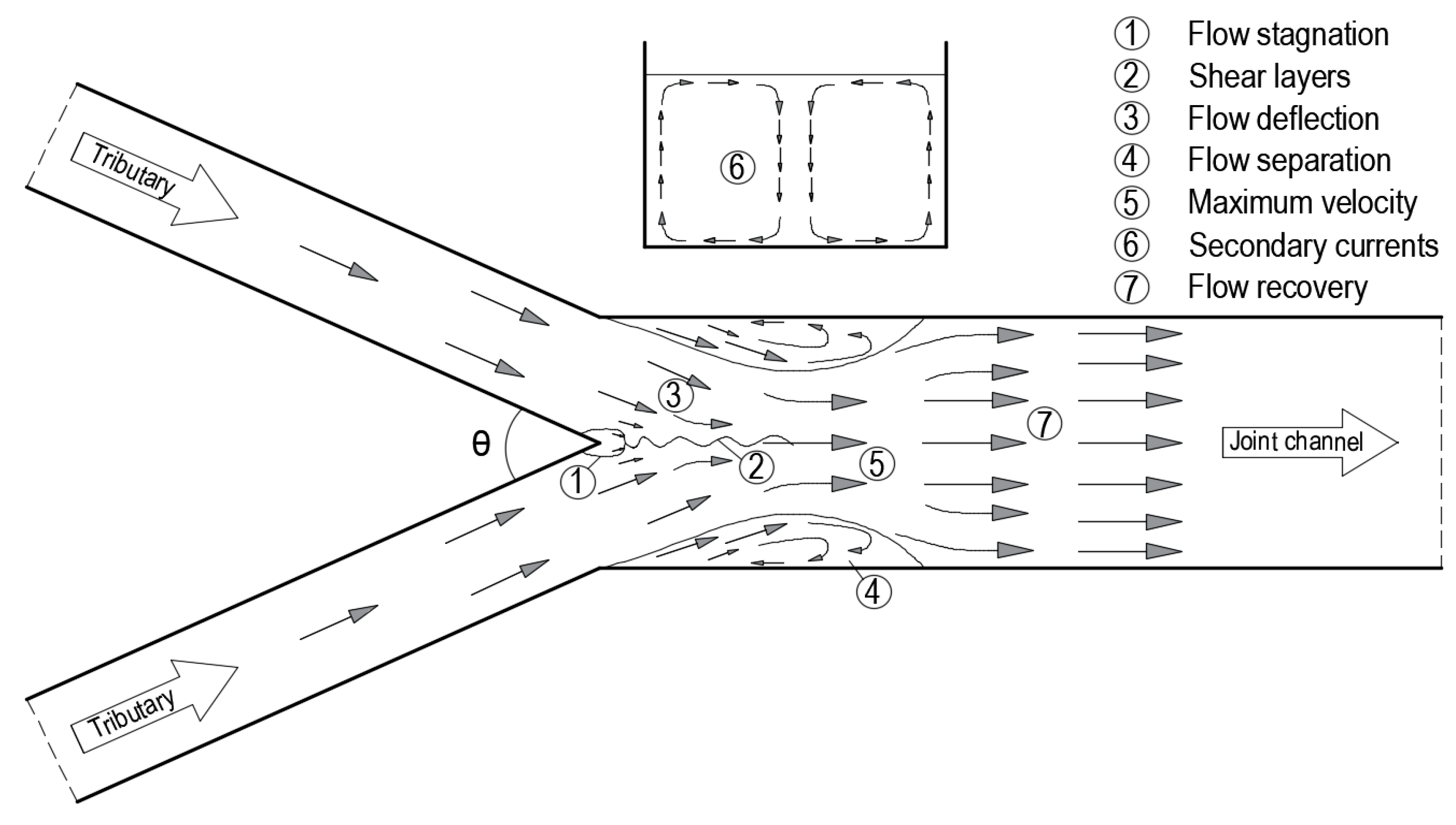
Best [4] identified six main flow elements in river confluences, namely: flow stagnation, flow deflection, flow separation, maximum velocity, flow recovery, and shear layers. Furthermore, Rhoads and Sukhodolov [5] and Riley and Rhoads [6] pointed out the formation of secondary currents induced by the lateral pressure gradient due to the deflection of the converging flows along the mixing interface. The regions where these flow elements take place are depicted in Figure 1 for symmetrical confluences.
These elements are recognized to influence the accumulation of contaminated sediments in some river locations ([7]) and they are mainly controlled by the junction angle, momentum and discharge ratio of the tributary flows and planform symmetry ([1,3,8]).
In symmetric confluences, the increase in junction angle, θ, leads to the increase in the flow stagnation and separation areas [6]. Riley and Rhoads [6] point out the strong influence of momentum ratio on the flow deflection. Yu et al. [7] investigated both morphodynamics and deposition patterns of contaminated sediments as a function of geometric and flow conditions and suggested that the junction angle and discharge ratio are crucial to understand the bed morphology and sediment transport pattern in confluences.
The numerical study conducted by Bradbrook et al. [9] highlighted the importance of junction angle, topographic forcing, and turbulence on the flow mechanisms in confluences. The authors explain the controls upon flow structure generation for laboratory and field confluences and identify the main factors for the characteristics of complex flow structures.
Yuan et al. [8] investigated the turbulent flow structure of in a confluence emphasizing the distortion of the shear layer. The study analyzed hydrodynamics and turbulence characteristics focusing on mean velocity field, Reynolds shear stress, turbulent kinetic energy, turbulence spectrum, and occurrence probabilities of quadrant events. The authors observed the development of strong helical cell in the cross sections when the tributary channel had a higher flow rate than the main channel. Reynolds shear stress, the maximum turbulent kinetic energy and occurrence probability of ejection and sweep events were mainly distributed within the middle zone of the water depth, rather than near the water surface, which is consistent with the distortion of shear layer. With a constant discharge ratio, an increase in the discharge of both channels resulted in an increase in velocity, turbulent kinetic energy, and the absolute values of Reynolds shear stress. The shear layer distortion is observed at a larger extent as the discharge of each channel decreased.
Rather different flow patterns can be observed if tributaries have different bed elevations (i.e., discordant confluences). De Serres et al. [10] studied the influence of momentum ratio in the flow mechanisms of confluence flows with discordant confluences. The authors identified the distortion of the mixing layer and a strong flow upwelling. The sediment transport and the riverbed morphology were associated to the vortices in the mixing layer zone. Canelas et al. [11] conducted an experimental campaign comprising two experiments with concordant and discordant beds between the tributaries. It was observed that, for the concordant bed case, the flow deflection occurred for the most part in the horizontal plan whereas for the discordant bed case, the wall-normal jet in cross-flow wraps around the tributary flow, exhibiting primarily vertical deflection in the direct vicinity of the inner bank. Boyer et al. [12] studied the flow structure in a discordance confluence and found that the bed step between the confluent rivers increases turbulence intensity and enhances upwelling of flow within the confluence.
Sukhodolov and Sukhodolova [13] studied the processes associated to the generation of secondary currents in confluences and found that the need for further systematic investigations of the effects of flow separation due to avalanche faces and topographical steering.
The effect of the ratio of the tributary to the main channel width on the flow structure in rectangular and trapezoidal channels at an asymmetric confluence was numerically studied in Azma and Zhang [14] who found that the width ratio has a significant effect on the flow structure and exchange of momentum between main and tributary flow at the confluence.
Guillén-Ludeña et al. [15] carried out an experimental study in a laboratory confluence with low discharge and momentum ratios to better understand the morphologic processes with narrow steep tributaries with high sediment load entering a wide low-gradient main channel. The authors highlight that the bed morphology presented typical features of discordant confluences, such as an avalanche face at the tributary mouth and a bank-attached bar along the inner bank of the post-confluence.
The flow mechanisms in fluvial confluences are complex and during recent decades, several studies were carried out to understand the behavior and the interactions between each tributary flow. The present study aims at understanding the flow mechanisms in confluences and the specific influences of tributaries widths and discharge ratios. The experimental study was carried out in a symmetric subcritical confluence where the tributaries joined at an angle θ = 50° to form a new downstream channel. Three-component velocity was collected with Acoustic Doppler velocimetry, and average and turbulent flow characteristics such as mean velocity field, turbulent kinetic energy, Reynolds shear stress, fluctuating velocity and secondary currents were analyzed. Moreover, main flow mechanisms such as development of shear layer or jet flow were identified. In addition, the influence of width ratios and discharge ratios in the turbulent flow structure and shear layer is presented.
Besides the flow characterization in confluences, the results may also be useful for validation of numerical simulations as they stand for six flow cases with different configurations (tributary widths) and discharges.
2. Materials and Methods
2.1. Experimental Apparatus
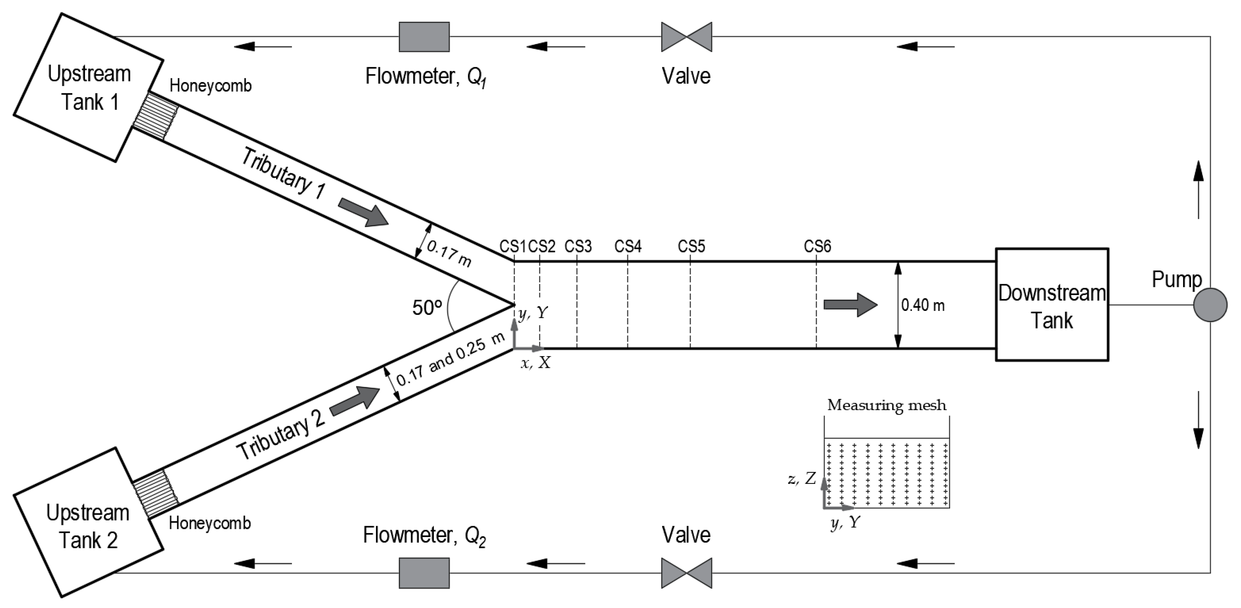
The experiments were conducted in an approximately 8 m-long symmetrical confluence flume at the National Laboratory for Civil Engineering (LNEC) in Lisbon, Portugal. The flume included two upstream concrete channels called tributaries 1 and 2 with widths (b1 and b2) equal to 0.17 and 0.25 m, respectively, and height equal to 0.25 m. Tributaries joined together with an angle of 50° and formed a new downstream concrete channel with width, b3, of 0.40 m and height equal to 0.15 m. In order to understand the influence of the tributary width, during the experimental campaign the width of tributary 2 was decreased to 0.17 m and a complete symmetrical configuration was obtained.
Figure 2 presents a schematic configuration of the experimental recirculating hydraulic circuit. Each tributary was fed by dedicated pipes that collect the water from a downstream tank and fill tanks 1 and 2. The flow discharges to tributaries 1 and 2, Q1 and Q2, were controlled by two valves and monitored by two electromagnetic flowmeters with a precision of 0.01 L/s.
In the very start of each tributary, the flow enters through a 3 cm-diameter circular honeycomb screen with a length of 30 cm and the same width and height as the channel, to ensure its alignment and stabilization with the longitudinal axis of each channel (cf. Smyk et al. [16]).
The subcritical flow depth is imposed by a downstream tailgate.
2.2. Control Variables and Parameters
The experimental campaign comprised five flow cases. Conditions and main bulk variables of each one are presented in Table 1.
In the table, subscripts 1 and 2 stand for tributaries 1 and 2, respectively. M stands for the momentum flux, calculated by M = ρQU, where ρ is the volumetric mass density, Q is the flow discharge and U is the average cross section velocity measured at a distance of 0.2 m from confluence to upstream; Fr is the Froude number calculated using , where g is the gravity acceleration and h is the flow depth, and Re is the Reynolds number calculated by , where R is the hydraulic radius and is the kinematic viscosity (an average value of 9.5 × 10⁻⁷ m2/s).
All experiments were carried out in steady flow, i.e., the flow discharge was kept constant in each flow case.
A Cartesian orthogonal coordinate system was used. The origin is at the right-hand side of the joint channel. The instantaneous velocity components u, v and w correspond to the longitudinal (x), transverse (y), and vertical (z) directions, respectively.
In order to make results comparable to other studies, whenever possible, joint channel width, Bm, and average cross-sectional velocity were used to normalize the corresponding variables. Therefore, X = x/Bm, Y = y/Bm and Z = z/Bm.
2.3. Equipment
Flow depths and velocities were measured within the confluence channel.
The flow depths were measured using ultrasonic-level probes (Baumer UNDK 30) which use the emission of an acoustic sonic frequency of 240 kHz to determine the distance from a given surface reflector with a maximum error of 0.5 mm. In each point, the measurements were performed for approximately 1 min with a frequency equal to 10 Hz. These measurements were complemented by measurements made with a point gauge. Flow depths were obtained by the difference between the bottom and the water surface elevations with both instruments. Water depths were measured in 10 cross sections that were located at 0, 10, 25, 35, 45, 70, 85, 120, 140, 180 cm from confluence.
Three component velocities were measured by means of a Nortek Vectrino Accoustic Doppler Velocimeter (10 MHz with a side-looking probe). The measurements were taken for 90 s with an acquisition frequency of 100 Hz. Six cross sections at downstream starting immediately after the joint of the two tributaries were surveyed as presented in Figure 2. In each cross section, a total of 10 verticals with 8 points each (equidistant in both directions), were used for flow characterization. Additionally, one cross section in each tributary was also surveyed. As recommended by the manufacturer, the signal-to-noise ratio (SNR) and the correlation were monitored and data with values bellow 15 dB and 70%, respectively, were discarded. To improve the acoustic signal reflection, silica powder was added to the flow as seeding whenever it was needed. Time-series velocity data were treated through the proposed change made by Walh [17] of the phase-space threshold despiking method developed by Goring and Nikora [18].
Automatic displacement was used to move equipment which allowed for the automatic positioning of the equipment in the lateral and vertical directions at a precision of 1 mm. Streamwise positioning was made manually.
3. Results
3.1. Water Depths
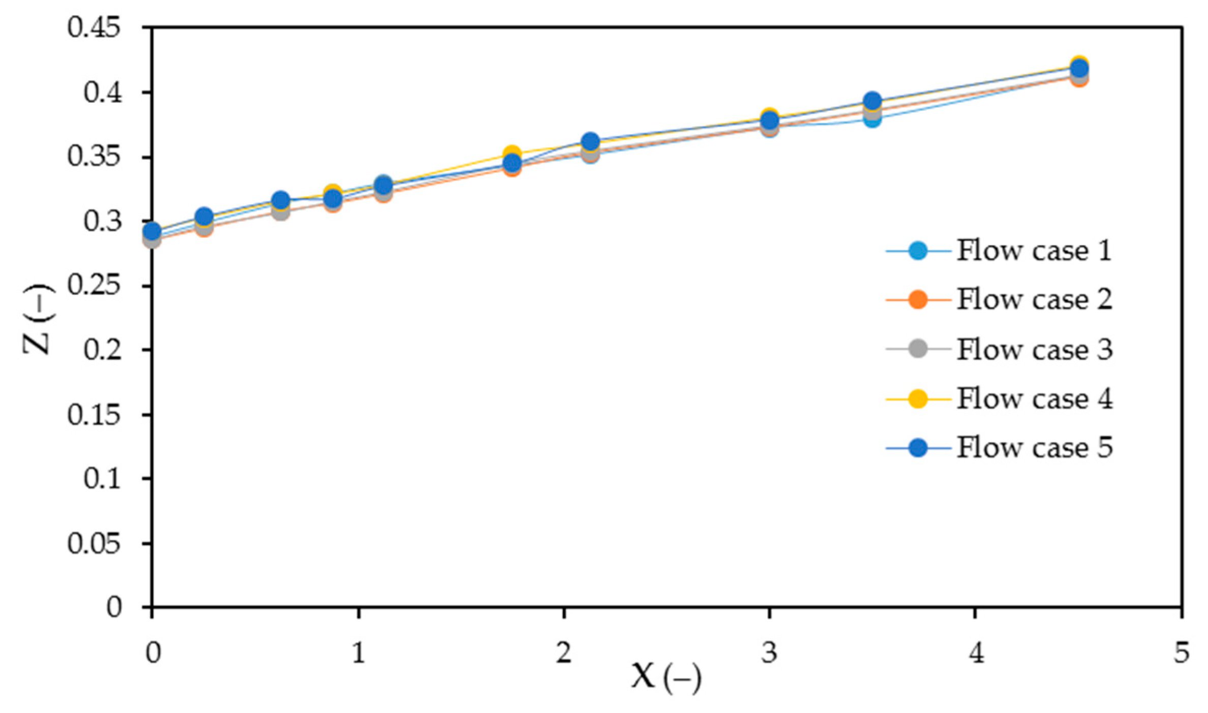
As can be shown in Figure 3, the longitudinal profile of water depth in the joint featured a rather similar pattern for all flow cases. There were no significant and clear differences between the results of the water depths due to the difference of tributary momentum and width ratios. In the present case, water depths (equal to approximately 0.1–0.12 m depending on the cross section) were mainly driven by the total discharge, channel geometry and roughness and downstream tailgate elevation. As all these characteristics and variables were the same for the five flow cases, the similarity in the water depths was not surprising. Furthermore, an influence of the tailgate was found in the longitudinal water depth profile, corresponding to a M1 curve of varied flow (see for instance [19]).
3.2. Mean Flow Characteristics
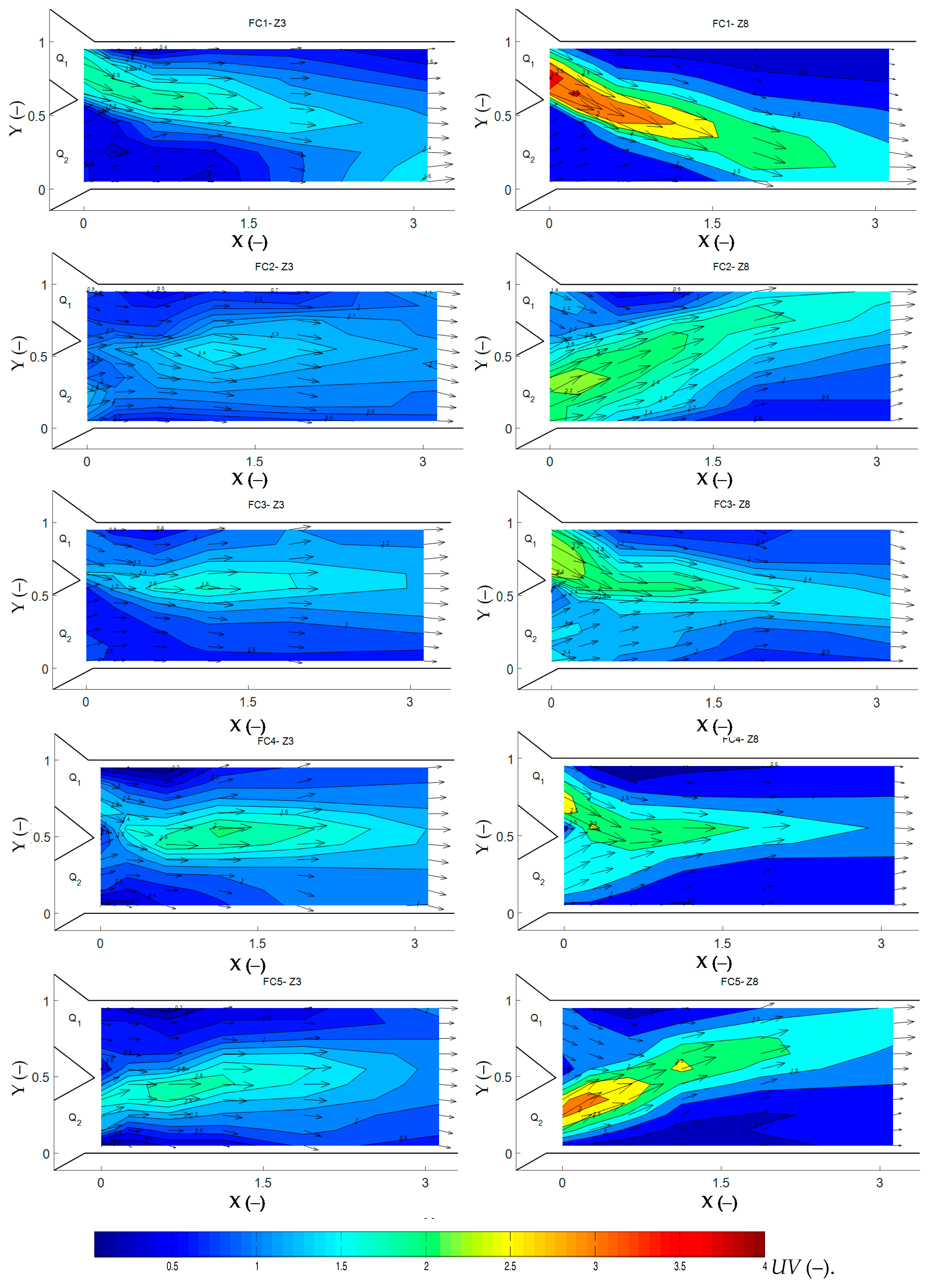
Figure 4 presents the plan view of the non-dimensional velocity magnitude UV, defined by and the velocity vectors u and v. The measurements were conducted in eight vertical positions, however for clear presentation, only plan views at Z = 3 and Z = 8 were plotted.
The dominant flow direction was clearly observed in the plots and it was particularly felt in the region near the water surface. These flow intensities near the surface, which were much higher than the flow intensities near channel bed, were attributed to the typical logarithmic streamwise velocity profiles signature in the single upstream tributary channels.
As can be seen in the Figure 4, tributary flows cannot remain attached to the wall in the joint confluence and in most cases, flow separation was formed near the lateral walls. This separation zone spread in the streamwise direction in accordance with the velocity magnitude which seems to depend mainly on the momentum ratio between the tributary flows. This flow element was observed in whole vertical plans. Near the channel bed, the strength of this separation zone was higher than near the surface where flow tended to move streamwise rather than forming separation area.
Flow deflection was observed as soon as the interaction between the tributary flows started. The direction of the velocity vectors in the plan view indicates this flow element. Further downstream and specifically in the last cross section, flow recovery was obtained and spanwise velocity is almost nil.
Regarding maximum velocity, it was particularly evident in the region near the channel bottom. Moreover, all these typical flow elements were recognized in the plots and will be further analyzed in Section 4.
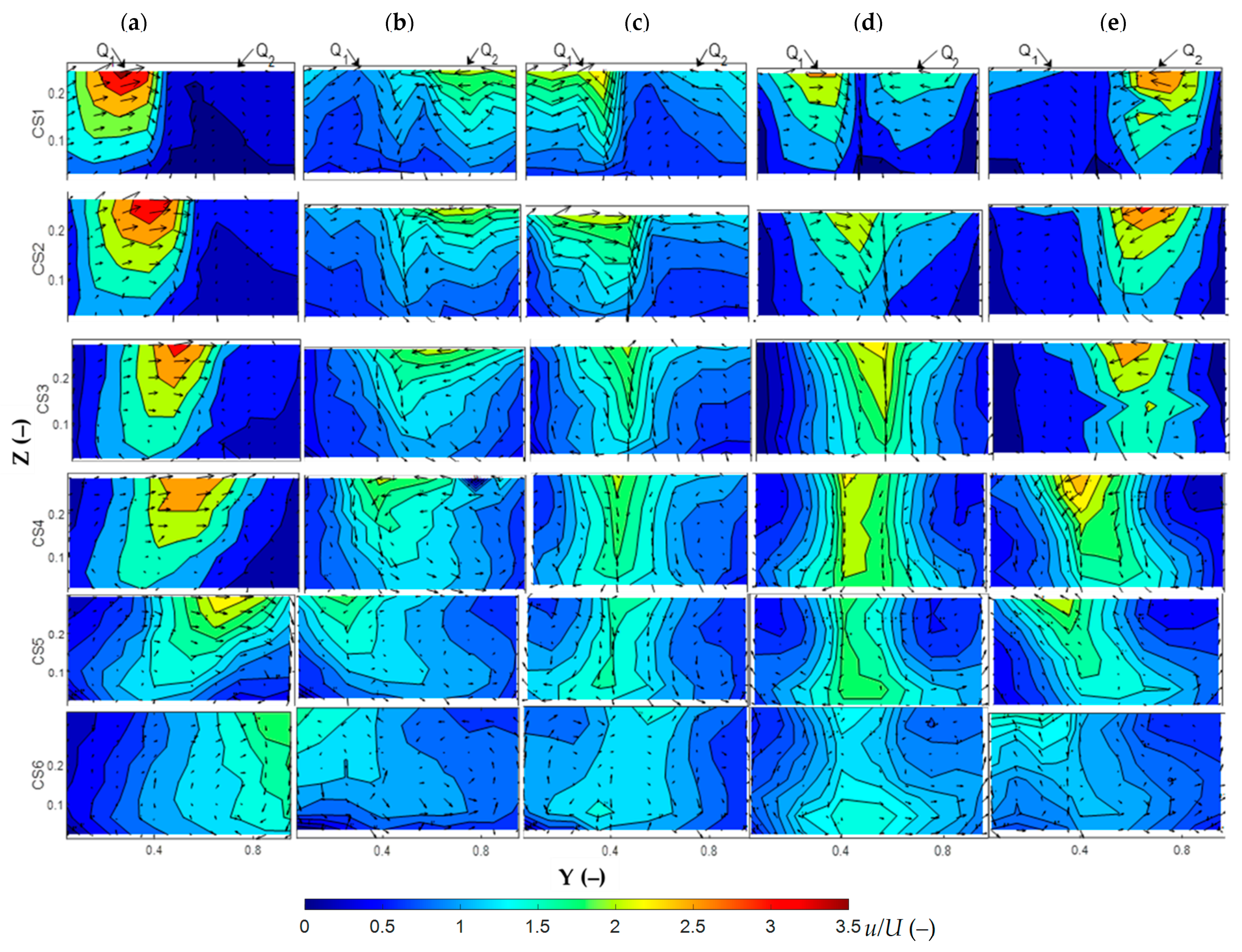
The cross-sectional distribution of the non-dimensional velocity magnitude Ux, defined by UX = u/U is presented in Figure 5. In the same figure, secondary current vectors (spanwise and vertical velocities) are also presented.
The cross-sectional velocity vectors reflected the secondary currents formed in the confluence joint channel. For every flow case, two secondary cells were observed in the first cross section. These cells stand for the two spiral jets with different magnitudes depending on the width and momentum ratio. Flow case 1 features high width and momentum ratio (Table 1) which leads to higher secondary velocities for tributary 1. Due to the much higher streamwise velocity from that tributary, especially near water surface, this secondary flow was transported downstream and eventually became the only secondary cells in the cross sections 2 to 6.
3.3. Turbulence
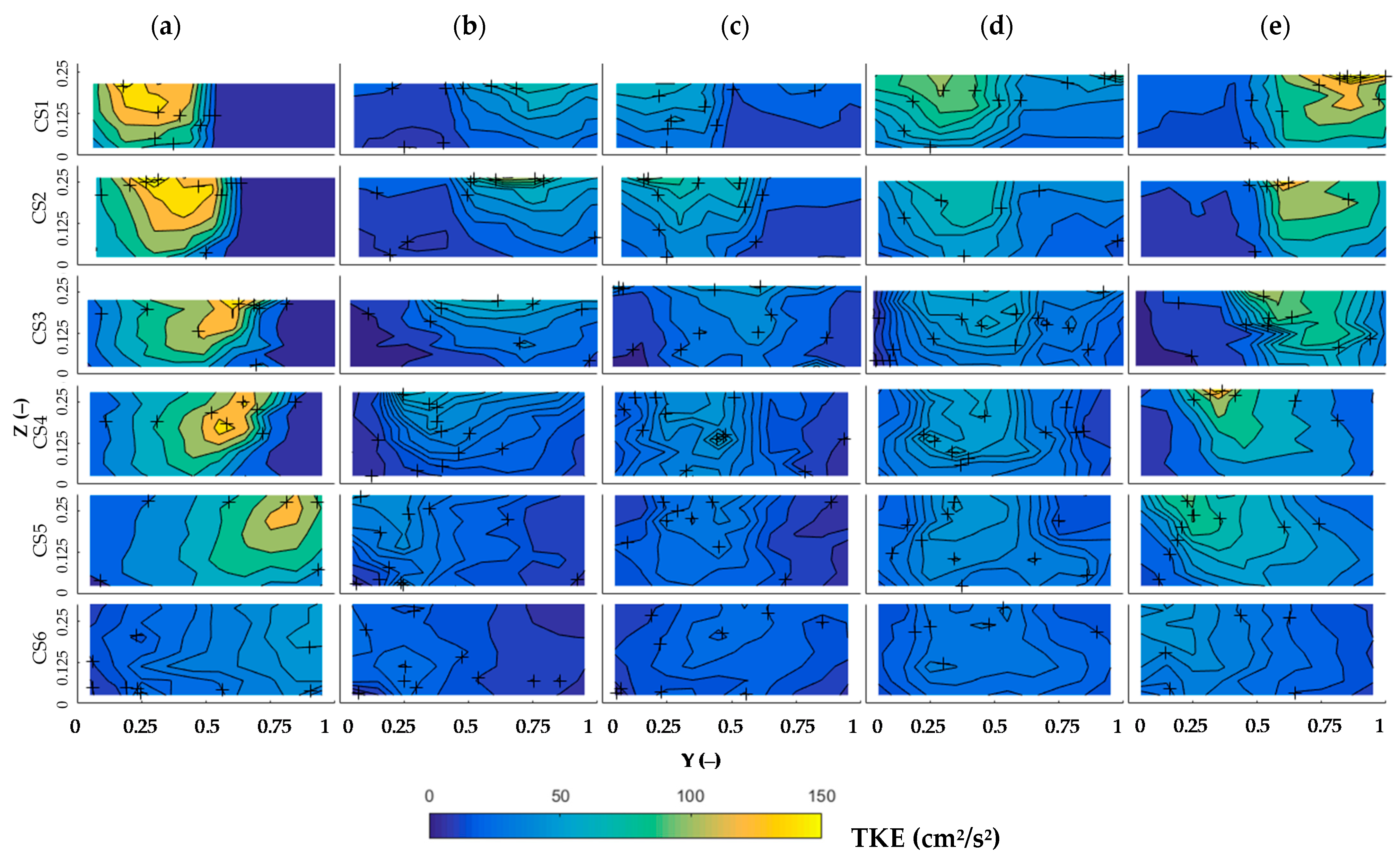
The turbulent kinetic energy, defined by , where , and are the fluctuating velocity components based on the Reynolds decomposition, is presented in Figure 6.
According to the figures, there are many factors which need to be taken into consideration, to begin with, TKE gradually decreased towards the channel wall, it was also decreased towards the bed. Maximum values of TKE occurred at a distance of 10 cm from the confluence. For flow case 1, given the big difference of momentum flow and velocity between two tributaries, there was a sharp jet flow which hit the wall approximately in cross section 6. For other flow cases jet flows were not as sharp as FC1 and the accelerated flow kept its path and slower flow bends to align itself with the higher momentum flow when two flow collided at an angle. As can be understood from the main flow elements in confluences by Best [4], external shear layers are formed between the two converging flows and internal shear layer are created between horizontal recirculation cell and the maximum velocity zone.
Magnitudes of turbulence kinetic energy decrease along the channel for all flow cases and intensity of TKE moves downwards and toward another tributary.
Momentum ratios for FC3 and FC4 are close together and contribute to two internal shear layers in cross section 1 and then they are going to mix and create one internal shear layer. External shear layers are formed between the two converging flows. Intensity of shear layers increases with increasing momentum ratio.
4. Discussion
Figure 1 presents the main flow elements that may be identified in symmetric confluence flows. The influence of tributaries discharge, momentum and width ratios on these flow elements is described herein. The interaction of the flows in the two tributaries with an angle close to the angle of the channels leads to the deflection of the flow towards the outer part of the channel wall. Together with this flow deflection, a stagnation area located in the junction between the tributaries is created. The presence of this area is clear for instance in Figure 4 for FC3- Z3. Despite the presence of the stagnation area over whole flow depth, this area is mostly evident near the joint channel bed as can be observed, for instance, in the cross-sectional streamwise velocity profiles for FC1.
Due to the relatively low angle between tributaries, reverse flows were not observed which is consistent with the criteria (e.g., [4], Figure 5).
In order to identify the trend of the flow deflection in the streamwise direction, the average cross-sectional deflection angle, β, defined by β =|tan−1(v/u)|, is plotted in Figure 7.
All flow cases present a similar trend.
As the angle of this symmetric confluence is 50°, the angle of each tributary with the joint channel is 25°. Without any interaction, it would be expected that this 25° could be observed in the first cross section (distance to upstream section of joint channel equal to zero). As the actual value is approximately equal to 13° to 15°, it is clear that the flow is influenced by the downstream conditions. FC1 features the higher average angle β.
The deflection of flows increases at both higher discharge and momentum ratios as observed in Figure 4.
In the present confluence, flow direction in the tributaries varies from the direction of the joint channel. Downstream of the confluence, the directions of the tributary flows are kept leading to a flow separation when these flows cannot remain attached to the channel due to the sharp change in wall geometry. The area occupied by this separation flow element is linked to the confluence angle as it determines the severity of the change of the boundary geometry (e.g., [4]). Analyzing data from Figure 4, flow separation follows the momentum ratio directly. Higher discharge and momentum lead to much higher flow separation in the side of the respective tributary.
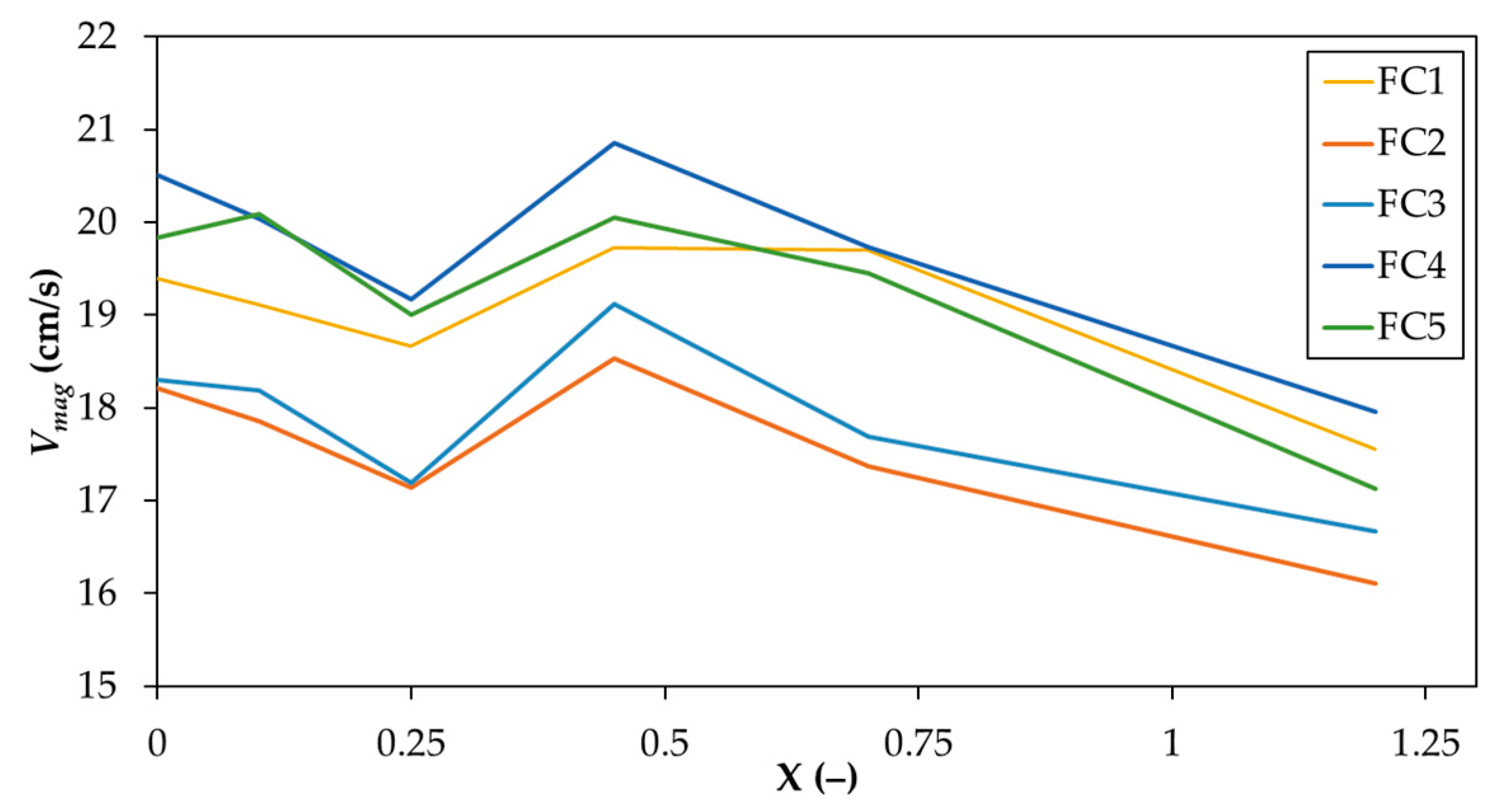
As referred to before, flow separation stands for an area close to the lateral joint channel where flow is hindered. This flow element reduces the effective flowing which leads to an increase in the local velocity. The velocity magnitude, Vmag is defined by Vmag = (u2+v2+w2)0.5 and cross-sectional maximum velocity is plotted against streamwise position in Figure 8.
Maximum velocity is observed for all flow cases. The streamwise position of this maximum velocity is approximately the same and corresponds to the area where flow separation is most evident.
In order to further analyze the secondary currents strength in the presented confluence channel, streamwise development of average cross-sectional velocity, (v2 + w2)0.5 was computed and plotted in Figure 9.
The experimental results obtained in this study are presented in Figure 4 and Figure 9 which reveal that the size, location and strength of the secondary currents are rather influenced by the momentum ratio. Furthermore, for most of the flow cases, two secondary counter rotating currents are observed. The strength of these currents has its maximum in the first cross section in the upstream part of the joint channel and diminishes downstream. For FC1, much higher momentum is transferred in tributary 1 which leads to the suppression of one secondary current. This jet flow coming from tributary 1 reached the right wall of joint channel in the last measurement cross section. The formation of the secondary currents is caused by the change of the flow direction due to flow deflection of both tributary flows. This deflection causes a surface radial pressure drop induced by the centrifugal force creating flow divergence towards the center on the surface and towards the wall near the channel bottom (e.g., Shakibainia [20]).
After the joining of the two tributary flows and the corresponding separation and deflection flow regions, velocity pattern becomes more aligned with streamwise direction. In this so-called recovery element of flow, turbulence intensities decrease, and flow becomes more stable when compared to region near the confluence.
5. Conclusions
Fluvial management should be based on the knowledge of the flow mechanisms in rivers. Among other configurations, confluences are important locations where sediment, velocities and directions of the tributary flows interact.
The flow mechanisms in a symmetrical confluence with a 50° junction angle were investigated. Flow cases comprised six conditions covering momentum, discharge and tributary channel width changes.
The hydrodynamic structures in the joint channel were found to be strongly influenced by the momentum ratio. By changing this ratio, variations on main flow elements in confluences were found.
As the experiment shows, at the beginning of the new channel, two internal shear layers are formed if the momentum difference was large which becomes an internal shear layer as the flow progresses.
Two spiral flows are formed by two tributaries in the new channel and in the end of channel they mix and create one spiral flow. According to the momentum ratio, different lengths are needed to form one spiral flow.
The increase in the flow separation is mainly influenced by the maximum flow velocity which is known to be important in the sediment transport and erosion in confluence flows. The sharpest jet flow belongs to the flow case 1, which has a largest discharge and momentum ratios; shear layer is also particularly marked for this flow case.
Author Contributions
J.F. proposed the theme and the setup and obtained the funding. L.A. conducted the experiments and wrote the frit version of the paper. J.F. and L.A. made a significant contribution to the research. All authors contributed to the final writing and revision of this paper. All authors have read and agreed to the published version of the manuscript.
Funding
This research was funded by FEDER and Science and Technology Foundation under the scope of the Project MixFluv–Mixing Layers in fluvial systems (PTDC/ECI-EGC/31771/2017).
Institutional Review Board Statement
Not applicable.
Informed Consent Statement
Not applicable.
Data Availability Statement
The data that support the findings of this study are available from the corresponding author, J.F., upon reasonable request.
Acknowledgments
Besides FEDER and FCT for funding this research, authors would like to acknowledge Nuno Aido and César Costa for the valuable help during the experiments and Juana Fortes from the Harbours and Maritime Structures Division of LNEC for the support on the experimental facility.
Conflicts of Interest
The authors declare no conflict of interest. The funders had no role in the design of the study; in the collection, analyses, or interpretation of data; in the writing of the manuscript, or in the decision to publish the results.
References
- Rice, S.; Roy, A.; Rhoads, B. River Confluences, Tributaries and the Fluvial Network, 1st ed.; John Wiley and Sons: New York, NY, USA, 2008. [Google Scholar]
- Webber, N.B.; Greated, C.A. An investigation of flow behaviour at the junction of rectangular channels. Proc. Inst. Civ. Eng. 1966, 34, 321–334. [Google Scholar] [CrossRef]
- Mosley, M.P. An experimental study of channel confluences. J. Geol. 1976, 84, 535–562. [Google Scholar] [CrossRef]
- Best, J.L. Flow dynamics at river confluences: Implications for sediment transport and bed morphology. In Recent Developments in Fluvial Sedimentology; Etheridge, F.G., Flores, R.M., Harvey, M.D., Eds.; SEPM Society for Sedimentary Geology: Tulsa, OK, USA, 1987; Volume 39, pp. 27–35. [Google Scholar]
- Rhoads, B.L.; Sukhodolov, A.N. Field investigation of three-dimensional flow structure at stream confluences: 1. Thermal mixing and time-averaged velocities. Water Resour. Res. 2001, 37, 2393–2410. [Google Scholar] [CrossRef]
- Riley, J.D.; Rhoads, B.L. Flow structure and channel morphology at a natural confluent meander bend. Geomorphology 2012, 163–164, 84–98. [Google Scholar] [CrossRef]
- Yu, Q.; Yuan, S.; Rennie, C.D. Experiments on the morphodynamics of open channel confluences: Implications for the accumulation of contaminated sediments. J. Geophys. Res. Earth Surf. 2020, 125, e2019JF005438. [Google Scholar] [CrossRef]
- Yuan, S.; Tang, H.; Xiao, Y.; Qiu, X.; Zhang, H.; Yu, D. Turbulent flow structure at a 90-degree open channel confluence: Accounting for the distortion of the shear layer. J. Hydro Environ. Res. 2016, 12, 130–147. [Google Scholar] [CrossRef] [Green Version]
- Bradbrook, K.F.; Lane, S.N.; Richards, K.S. Numerical simulation of three-dimensional, time-averaged flow structure at river channel confluences. Water Resour. Res. 2000, 36, 2731–2746. [Google Scholar] [CrossRef] [Green Version]
- De Serres, B.; Roy, A.G.; Biron, P.M.; Best, J.L. Three-dimensional structure of flow at a confluence of river channels with discordant beds. Geomorphology 1999, 26, 313–335. [Google Scholar] [CrossRef]
- Birjukova Canelas, O.; Ferreira, R.M.L.; Guillén-Ludeña, S.; Alegria, F.C.; Cardoso, A.H. Three-dimensional flow structure at fixed 70° open-channel confluence with bed discordance. J. Hydraul. Res. 2019, 58, 434–446. [Google Scholar] [CrossRef]
- Boyer, C.; Roy, A.G.; Best, J.L. Dynamics of a river channel confluence with discordant beds: Flow turbulence, bed load sediment transport, and bed morphology. J. Geophys. Res. Earth Surf. 2006, 111, F04007. [Google Scholar] [CrossRef]
- Sukhodolov, A.N.; Sukhodolova, T.A. Dynamics of flow at concordant gravel bed river confluences: Effects of junction angle and momentum flux ratio. J. Geophys. Res. Earth Surf. 2019, 124, 588–615. [Google Scholar] [CrossRef]
- Azma, A.; Zhang, Y. Tributary channel width effect on the flow behavior in trapezoidal and rectangular channel confluences. Processes 2020, 8, 1344. [Google Scholar] [CrossRef]
- Guillén-Ludeña, S.; Franca, M.J.; Cardoso, A.H.; Schleiss, A.J. Hydro-morphodynamic evolution in a 90° movable bed discordant confluence with low discharge ratio. Earth Surf. Process. Landf. 2015, 40, 1927–1938. [Google Scholar] [CrossRef]
- Smyk, E.; Mrozik, D.; Wawrzyniak, S.; Peszyński, K. Tubular air deflector in ventilation ducts. In Proceedings of the 23rd International Conference Engineering Mechanics 2017, Svratka, Czech Republic, 15–18 May 2017. [Google Scholar]
- Wahl, T.L. Discussion of “despiking acoustic doppler velocimeter data” by Derek G. Goring and Vladimir I. Nikora. J. Hydraul. Eng. 2003, 129, 484–487. [Google Scholar] [CrossRef] [Green Version]
- Goring, D.G.; Nikora, V.I. Despiking acoustic doppler velocimeter data. J. Hydraul. Eng. 2002, 128, 117–126. [Google Scholar] [CrossRef] [Green Version]
- Chanson, H. Hydraulics of Open Channel Flow: An Introduction—Basic Principles, Sediment Motion, Hydraulic Modeling, Design of Hydraulic Structures, 2nd ed.; Butterworth Heinemann: Queensland, Australia, 2004. [Google Scholar]
- Shakibainia, A.; Tabatabai, M.R.M.; Zarrati, A.R. Three-dimensional numerical study of flow structure in channel confluences. Can. J. Civ. Eng. 2010, 37, 772–781. [Google Scholar] [CrossRef]
Figure 1.
Flow elements in symmetrical confluences (adapted from adapted from [6]).
Figure 1.
Flow elements in symmetrical confluences (adapted from adapted from [6]).

Figure 2.
Schematic representation of the confluence flume.

Figure 3.
Longitudinal profile of water depths.

Figure 4.
Non-dimensional time averaged velocity magnitude UV and velocity vectors u and v.

Figure 5.
Cross-sectional distribution of the non-dimensional velocity magnitude Ux and vectors of spanwise and vertical velocities, (a) FC1, (b) FC2, (c) FC3, (d) FC4, (e) FC5, 6 lines correspond to cross sections CS1 to CS6 (as presented in Figure 1).
Figure 5.
Cross-sectional distribution of the non-dimensional velocity magnitude Ux and vectors of spanwise and vertical velocities, (a) FC1, (b) FC2, (c) FC3, (d) FC4, (e) FC5, 6 lines correspond to cross sections CS1 to CS6 (as presented in Figure 1).

Figure 6.
Cross-sectional distribution of the turbulent kinetic energy for flow cases, (a) FC1, (b) FC2, (c) FC3, (d) FC4, (e) FC5, 6 lines correspond to cross sections CS1 to CS6 (as presented in Figure 1).
Figure 6.
Cross-sectional distribution of the turbulent kinetic energy for flow cases, (a) FC1, (b) FC2, (c) FC3, (d) FC4, (e) FC5, 6 lines correspond to cross sections CS1 to CS6 (as presented in Figure 1).

Figure 7.
Longitudinal profiles of average cross-sectional deflection angle.

Figure 8.
Longitudinal development of cross-sectional maximum velocity.

Figure 9.
Secondary currents (v2 + w2)0.5.


Table 1.
Bulk flow variables for each flow case (FC).
| Flow Case | b1 (m) | b2 (m) | Q1 (L s−1) | Q2 (L s−1) | Q2/Q1 | M1 (kg m s−2) | M2 (kg m s−2) | M1/M2 | Fr1 | Fr2 | Re1 (×104) | Re2 (×104) |
|---|---|---|---|---|---|---|---|---|---|---|---|---|
| FC1 | 0.17 | 0.25 | 7 | 3 | 0.4 | 2.86 | 0.33 | 8.6 | 0.60 | 0.14 | 7.94 | 2.69 |
| FC2 | 0.17 | 0.25 | 3 | 7 | 2.3 | 0.49 | 1.79 | 0.23 | 0.24 | 0.34 | 3.29 | 6.29 |
| FC3 | 0.17 | 0.25 | 5 | 5 | 1 | 1.35 | 0.90 | 1.5 | 0.39 | 0.23 | 5.44 | 4.46 |
| FC4 | 0.17 | 0.17 | 5 | 5 | 1 | 1.32 | 1.34 | 0.98 | 0.38 | 0.39 | 5.36 | 5.41 |
| FC5 | 0.17 | 0.17 | 3 | 7 | 2.3 | 0.48 | 2.62 | 0.18 | 0.23 | 0.54 | 3.22 | 7.56 |
Publisher’s Note: MDPI stays neutral with regard to jurisdictional claims in published maps and institutional affiliations. |
© 2021 by the authors. Licensee MDPI, Basel, Switzerland. This article is an open access article distributed under the terms and conditions of the Creative Commons Attribution (CC BY) license (http://creativecommons.org/licenses/by/4.0/).
Share and Cite
MDPI and ACS Style
Alizadeh, L.; Fernandes, J. Turbulent Flow Structure in a Confluence: Influence of Tributaries Width and Discharge Ratios. Water 2021, 13, 465. https://doi.org/10.3390/w13040465
AMA Style
Alizadeh L, Fernandes J. Turbulent Flow Structure in a Confluence: Influence of Tributaries Width and Discharge Ratios. Water. 2021; 13(4):465. https://doi.org/10.3390/w13040465
Chicago/Turabian StyleAlizadeh, Leila, and João Fernandes. 2021. "Turbulent Flow Structure in a Confluence: Influence of Tributaries Width and Discharge Ratios" Water 13, no. 4: 465. https://doi.org/10.3390/w13040465
Note that from the first issue of 2016, this journal uses article numbers instead of page numbers. See further details here.