
Morphometry-Driven Divergence in Decadal Changes of Sediment Property in Floodplain Water Bodies
by
Pongpet Pongsivapai
1,*, 
Junjiro N. Negishi
2,*, 
Hokuto Izumi
1,
Paolo A. Garrido
1 and
Kanta Kuramochi
3 1
Graduate School of Environmental Science, Hokkaido University, Sapporo, Hokkaido 060-0810, Japan
2
Faculty of Environmental Earth Science, Hokkaido University, Sapporo, Hokkaido 060-0810, Japan
3
Graduate School of Agriculture, Hokkaido University, Sapporo, Hokkaido 060-8589, Japan
*
Authors to whom correspondence should be addressed.
Water 2021, 13(4), 469; https://doi.org/10.3390/w13040469
Submission received: 24 December 2020
/
Revised: 28 January 2021
/
Accepted: 5 February 2021
/
Published: 11 February 2021
(This article belongs to the Special Issue Endangered Freshwater Ecosystems: Threats and Conservation Needs)
Abstract
:Sediments are potentially the internal source that supply nutrients to water in lentic to semi-lentic ecosystems. The understanding of factors that cause temporal changes in sediment properties is critical for the internal source management. This study investigated the spatial variations and temporal changes in sediment properties in relation to their controlling factors in water bodies of the Ishikari River, Northern Japan. Sediment data in 29 water bodies were measured twice (around 2005 and 2019) to study the temporal changes in sediment properties, and were compared using Generalized Linear Mixed Models (GLMMs). The controlling factors of sediment properties including catchment and morphometry were examined by partial least square (PLS) regression. Our results showed that the temporal change in sediment properties over decades was largely driven by morphometry, while land use in the catchment played a relatively minor role in those changes. The rate of change in organic matter (OM) differed among water bodies depending on their morphometry. The small and shallow water bodies provided suitable habitat for macrophytes that led to OM deposits, resulting to an increase in OM and OM to total nitrogen (TN) ratio over time. The consequences of these changes are important for internal source management and biodiversity conservation.
1. Introduction
The understanding of sediment quality is the key for internal nutrient management of lentic ecosystems such as lakes and ponds. These water bodies receive mixtures of organic and inorganic materials that are transported from a variety of sources including the catchment and atmosphere, as well as those generated in situ by primary producers such as macrophytes and algae [1]. While a part of the inputs is exported further downstream or returned to the atmosphere, the remainder are deposited therein continuously, eventually becoming sediment at the water bottom [2,3]. Nitrogen (N) and phosphorus (P) are the major limiting nutrients for primary production [4] and are major constituents of sediment in organic forms or being adsorbed to sediment particles [2]. The deposited sediment is referred to as an internal source due to sediment-associated N and P supplied to the water column, depending on the complex biogeochemistry at sediment-water interface [5,6,7]. The effects of internal sources, in particular P, on water quality and ecosystem processes are substantial by mediating primary production and food web interactions [8], which can delay restoration processes for many years even after external stressors are controlled [6,9]. In addition, carbon (C) stored in burial in lentic systems acts as an important sink in the global C cycle as well as eutrophication of water [10]. Therefore, successful implementation of management efforts aimed at reducing such algal blooms requires an integrated approach, including both external and internal nutrient loads, and C storage [11,12].
Lentic water bodies found in floodplains (floodplain water bodies; hereafter FWBs) include various types such as natural and artificial oxbow lakes, and back marsh in contemporary human-altered landscape [13]. These water bodies have continued providing important functions for living organisms, making floodplains a biodiversity hotspot [14,15]. Historically, riverine floodplains were the areas of sediment and nutrient deposition associated with recurring flood inundations and lateral movements of river channels with high fluvial dynamics and groundwater processes [16]. However, man-made processes altered the hydrological connectivity by building flood dykes or attenuating high flows in the main channel which increased the isolation of FWBs [14,15]. Furthermore, land use activities in surrounding or upstream areas provide additional stressors by loading excessive pollutants and sediment [17]. Overall, the loss of biodiversity has been reported in FWBs worldwide [18]. Despite the abundance of scientific knowledge on water quality and biological community that largely concluded the need of attention on external sources of nutrient and hydrological connectivity [19,20,21]. Yet only few studies conducted in FWBs have focused on sediment quality [22]. Given the importance of sediment in lentic ecosystems, this gap needs to be filled to implement efficient restoration and conservation efforts in FWBs.
A myriad of potential controlling factors exists for spatial patterns of sediment quality across FWBs. Firstly, matter inputs from external sources can directly lead to changes in the characteristics of accumulated sediment. Agricultural and/or urban areas in the catchment generally induce downstream changes in water quality and sediment in aquatic systems, with different impacts depending on the proportion of land use type in each system [23,24,25]. Similar land-water linkages have been reported for FWBs and lakes in studies on water quality and sediment [20,22,26]. For example, a proportion of agricultural activities associated with the amount of N and P in water and/or sediment of receiving water bodies. Second, the retention capacity of water bodies, which can be affected by the ratio between the size of catchment and receiving water (also known as drainage ratio), affects the extent of land influences on water quality partially depending on spatial scales examined [27,28]. Third, the morphometric features of FWBs such as depth and size of surface water can have decisive effects on the functionality of an entire ecosystem, which include generations of heterogeneity in sediment deposits via changes in quality and quantity of primary producers. For example, shallow water tends to provide a more suitable habitat for macrophytes and thus may promote plant succession and deposits of detritus that may differ from those originating from phytoplankton [13,29].
Sediment quality and quantity are not temporally constant even without additional accumulation of deposits. It is maintained and modulated through complex physical and biogeochemical processes. The mineralization of organic matter (OM) is among the key processes in such dynamics [30]. High organic matter content in sediment can provide energy source for microorganisms which play an important role in mineralization as main decomposers [31]. Organic C, N, and P in sediment can breakdown to soluble forms by a mineralization process that can decrease OM and nutrients in sediment [32]. Furthermore, mineralization can decrease C:N ratio over time [33,34]. In contrast, the mineralization rate of OM in sediment can be affected by various factors of such as oxygen level [32,35], temperature [36], iron content (Fe) [37], C:N ratio [35,36], and OM source [36]. Moreover, there are interactions among the characteristics of sediment. When N is concerned, sediment-associated N is largely contained in the form of organic matter [32]. In contrast, P abundance in sediment (P-fixation) is strongly associated with the characteristics of inorganic particles [32,38] and the retention capacity and sorption efficiency of P to sediment is partly controlled by the amount of OM, Aluminum (Al), Fe, and Calcium (Ca) content in sediment [39]. Temporal change in these external and internal controlling factors of sediment can cause temporal changes in quality of bed-surface sediment [40,41].
The Ishikari floodplain is a highly heterogeneous system which contains different types of FWBs such as marsh and natural oxbow lakes with high diversity in morphometry [13,42]. It also harbors the remnants of its historical landscape of this kind in Japan. Increasing human pressures have been reported in the fish community and water chemistry through introduced fish species, increasing nutrient sediment loading from agricultural fields [20,43,44], while a diversity in environmental conditions among FWBs continues provides diverse habitat for aquatic organisms [45,46]. As far as sediment is concerned, the accumulation rates of fine sediment from surrounding fields were shown in several selected water bodies [26]. However, these previous findings have not been well integrated into qualitative aspects of sediment, which has important relevance to water quality and food web. The Ministry of Land, Infrastructure, Transport and Tourism (MLIT) promotes a comprehensive plan of restorations and conservation of floodplain areas in lowlands of the Ishikari River [47]. The knowledge gap in spatial and temporal patterns of sediment quality needs to be filled. Thus, the objective of this study was to examine spatial as well as temporal patterns of sediment properties in FWBs in relation to external and internal environmental factors. Data collected 13–15 years ago was compared with the findings of a survey in 2019 to assess the temporal changes at decadal scale. We hypothesized that the intensity of agricultural activities in catchments, as well as morphometry, would be reflected in sediment quality. Specific predictions were as follows: 1) nutrient contents and OM contents would be correlated with the agricultural land use in catchment in both data types; 2) positively for nutrients and negatively for OM; 3) the changes in sediment property would be disproportionately higher in sites with high land proportions of agricultural activities in catchments with shallow water and high drainage index.
2. Materials and Methods
2.1. Study Sites
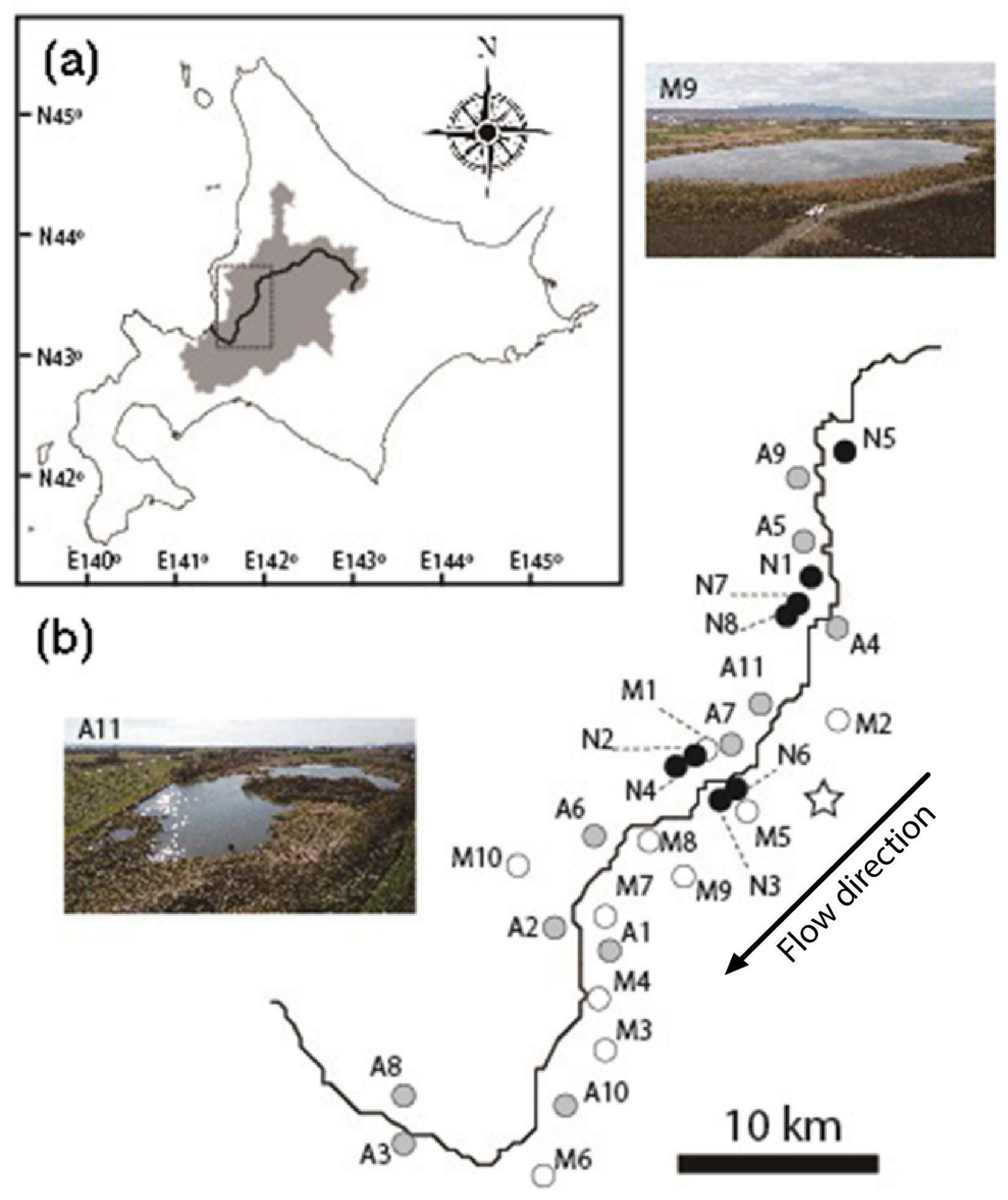
The study was conducted along a 60 km stretch of lowland section of the Ishikari River (catchment area: 14,330 km2) (Figure 1). Mean annual precipitation and temperature recorded in the closest weather station (Bibai station of Japan Meteorological Agency; 43°21’51.8” N 141°49’40.3” E) for the study period of 2004–2019 were 1178.47 mm and 7.53 °C, respectively. Currently, the major land use types in the Ishikari River watershed include forest, agricultural, and urban areas, the largest being forest and the smallest being urban areas [48]. Historically, the study area formed a vast wetland underlain by peat land (peat mire) [13,20]. Peatlands were largely transformed to agricultural areas between the 1950s and 1960s [20,26]. Moreover, flood levees were constructed along both sides of the river together with extensive channel-straightening river works to protect farmlands from natural flooding and to consolidate fragmented farmlands [13,26]. Consequently, most of the peatlands disappeared and the most dominant land use type in the surrounding area of FWBs were paddy fields for rice and crop lands for wheat [20].
We investigated numerous FWBs that were present, several were originally pools in peat mire formed in the peatland, which was later converted into water bodies used for irrigation and drainage activities, whereas others are the remnants of oxbow lakes [20,49]. Non-oxbow FWBs, including those probably originating from peat mire, were referred to as backmarsh (hereafter, marsh) because the flooding of the main channel and resultant formation of waterlogged areas probably have contributed to the formation of marsh water bodies [43]. Furthermore, oxbow lakes were classified into natural and artificial (hereafter, natural and artificial oxbow lakes), the latter of which were formed by river straightening works [13]. It was probable that these FWBs were occasionally connected to the main channel through flood inundation historically. In the present, flood control measures such as dams in upstream and embankment reduced the connectivity to almost nil. The study area has not been inundated from flooding of the main channel since 1980s, thus it was assumed that depositional condition of sediment in FWBs were not altered by factors other than those considered in this study.
Twenty-nine FWBs consisting of three types with different formation processes were selected (Figure 1, Table 1). According to the trophic state categories by Smith [4] in the level of total phosphorus, the study FWBs were either “eutrophic” or “hypertrophic”. Nutrient flux transferred from the catchment to the FWBs takes place mainly in springtime (March to May) due to snow melt and soil preparation for paddy field [20]. In the period from summer to autumn (June to November), which partially overlap with non-irrigation period (typically starting from August), external sources are reduced due to less agricultural activities [20]. The relatively high temperature and possible contribution of internal nutrient sources result in high primary production in planktonic algae with high chlorophyll a level in surface water during summer [50]. In addition, there is a possible contribution of nutrients from migrating waterfowls [51]. Moreover, the different lake morphometry among FWB types caused variable macrophyte distribution, as controlled by average depth and slope of littoral zones [13]. Consequently, macrophytes were considered among major contributors of autochthonous production of organic matter besides algae particularly in relatively shallow FWBs.
2.2. Sediment SAMPLING and Properties
The sediment sample was collected by MLIT (MLIT, unpublished data) between 2003 and 2006 (Table 1) and the data from this source was hereafter referred to as MLIT data. Sediment was collected again on 3–6 September 2019 with the same method at the same location described in the MLIT data; this was referred to as 2019 data. Surface layer of the sediment (0–10 cm) was collected at the approximate central point of the water surface in each FWB using an Ekman-Birge Grab sampler. When signs of disturbance of sediment in the sampler were observed, the sampling was repeated in slightly different spots until undisturbed samples were collected. Collected sediment was mixed in situ. Subsample was immediately transported to the laboratory in an ice chest and stored 4 °C until chemical analyses within four months.
The sediment properties were determined by adapting as similar analytical methods for MLIT data and 2019 data as possible. Wet sediment samples with three replicates for each FWB that passed through a 2 mm sieve were analyzed for water content, OM, total N (TN), and total P (TP). The OM in sediment was determined by loss on ignition method by combusting dry samples at 600 °C for 2 h. The TN (mg/g) of wet sediment was determined by semi-micro Kjeldahl method after digestion with sulfuric acid. For TP, wet sediment samples were digested through mixed sulfuric-nitric acid. The aliquots from digestion were used to determine TP (mg/g) by molybdenum-blue method and measured for the absorbance value with UV-visible spectrophotometer (UV-1280, SHIMADZU Co., Kyoto, Japan) at a wavelength of 880 nm. Water content was used to calculate TN and TP in dry weight. C:N ratio, which is used as an index of OM quality [34,52], was not available. Instead, proportional amount of TN in OM (OM to TN ratio) was calculated as a proxy indicator of OM quality. Lastly, TN to TP ratio was obtained as another quality index of sediment.
2.3. Catchment and FWB Characteristics
Landscape characteristics for each FWB were quantified based on land use composition in contributing area (catchment). We used nation-wide land use census data (land use database, MLIT, 100 m grid resolution: https://nlftp.mlit.go.jp/ksj/index.html) for all available years relevant to the study (years 1996, 2006, 2009, and 2016), the total areas of following land use types were obtained using ArcMap (Ver. 10, ESRI Co., Redlands, CA, USA): paddy field, crop land, urban area, and wetland. The proportion of each of these land use types in catchments were derived as a percentage in total catchment area.
Total catchment area was estimated in several ways as the relationship between water and land can be affected by varying spatial scales of observation [22]. First, drainage channels, which were artificially made to drain water from agricultural fields and river channels contributing to each FWB were identified by aerial photos, field visits and consultations with local landowners and management authorities (Figure S1a in Supplementary Materials). Second, for contributing river channels if there were any, a topographically defined watershed was generated by the hydrology function of ArcMap. Channel-buffer catchment area was calculated as the total area of buffer strips on both sides of all contributing channels and water perimeter buffers of each FWB; this area was merged in ArcMap and defined for two spatial scales at 100 m and 200 m buffer width (Figure S1b,c). Watershed-integrated catchment area was calculated as the total area of buffer strips on both sides of drainage channels, entire watershed areas for river channels and water perimeter buffers of each FWB; this was processed as done for channel-buffer catchment area (Figure S1d). These four methods were considered appropriate because previous studies on water-land interactions including one in the study region adapted a buffer spatial scale of several hundred meters and demonstrated that watershed-scale land use could be the important spatial extent influencing the physio-chemical conditions of receiving water bodies [20,53]. An assumption was made that the total catchment area of FWBs remained temporarily constant over the study period regardless of the methods used in estimates. In total, four types of land use data were prepared for each year for further analyses.
Surface areas (m) of FWB were estimated similarly as it was conducted in Negishi et al. [13]. An acoustic sonar device (Deeper Smart Sensor PRO+, Deeper, UAB, Lithuania) was used to measure average water depth (m) by taking measurements from water surface at approximately equally distant 3–5 spots across each FWB in sediment collection of 2019. The water volume (m3) of each FWB was calculated by average depth multiplied by their surface areas. The changes of depth and surface area over the study period were not significant as tested in preliminary examination of data; constant values were used for further analyses. As an index of how much matter was retained relative to the potential in outflow via hydrological exports, drainage ratio (i.e., ratio of catchment area to the surface area) has been often used [28]. The study FWBs varied much in terms of depth even for comparable size in surface water and ordinary drainage ratio was inappropriate for this purpose (Table 1). Thus, drainage index was instead used to represent retention capacity of FWBs; it was defined as a ratio of catchment area to the water volume, in order to reflect that fact that waterbodies having similar surface area had a wide range of water depth and retention capacity can be inaccurate by the use of traditional approach using drainage ratio. Moreover, land-use specific drainage index was calculated for paddy fields, crop lands, and urban areas to identify loading potential of matter influxes from different land use types.
2.4. Statistical Analyses
To examine whether land use composition in the catchment changed over the study period, generalized linear mixed model (GLMM) was developed with the percentage of respective land use types in catchment as a response variable, with independent effects of year of observation, and spatial scale of buffer delineation (100 m or 200 m), and land use type, as well as interaction effects of all the combinations of them as main factors. The identity of water bodies was included as a random factor. The models were separately developed for two types of catchment delineation methods (channel-buffer catchment and watershed-integrated catchment). These full models were compared with the null models that excluded all the effects of observation year using likelihood ratio tests. When two models showed insignificant differences, temporal changes in land use composition were considered negligible regardless of the catchment delineation methods.
To examine the differences in catchment land use characterization in relation to spatial scale of buffers and catchment delineation methods (in total, four different estimates), the proportions of each land use in each FWB were obtained for each observation year and tested for correlations between all the combinations of four estimates using Spearman Rank’s correlation. Strong correlations with high statistical significance were interpreted that the use of different estimates had negligible effects in the relationships between catchment characteristics and sediment properties.
The temporal changes in sediment properties were examined by GLMMs with data type (MLIT data and 2019 data) as the main factor, and the identity of water bodies as a random factor. The significance of the main factor was tested by likelihood ratio tests between the models with and without main factor.
Environmental variables that affected sediment properties were examined using partial least square (PLS) regressions. This is a powerful and useful tool to determine multivariate relationship between a response variable and several explanatory variables in which the latter were partially correlated to each other (multi collinearity) [54]. Sediment property variables were separately examined for each data type (MLIT data and 2019 data). When OM was a response variable, nine variables, i.e., average depth, volume and drainage index, three drainage indexes specific to land use types, and proportion of three land use types, were included. When other response variables were response variables, OM was also added as a response variable because other properties could be affected by OM. In the analyses focusing on MLIT data, mean proportions of each land use type between 1997 and 2006 was used whereas the mean between 2009 and 2016 was used to analyze 2019 data. This approach was adopted because the sediment properties were assumed to have integrated effects of land use activities over multiple years rather than single years.
Environmental variables that affected the change rate of sediment property (percentage changes in sediment properties in 2009 data compared to those in MLIT data) were also examined using PLS regressions. Change rate was standardized across FWBs by dividing the rate by the number of years between two data sets (Table 1). As the explanatory variables, nine variables were included for OM as done above. For other sediment properties, the change rate of OM was also included in the model. To examine further the univariate relationships between OM and other sediment properties, generalized linear models (GLMs) were developed with the OM change rate as an explanatory variable and others as response variables. Lastly, principal component analysis (PCA) was carried out to examine the change rate patterns in relation to water body types, as well as other environmental variables that were important in PLSs on the spatial variation of sediment properties in two data sets.
All the statistical analyses were conducted in R [55] with packages “glmmADMB” and “pls”. Statistical significance was assessed at the level of p = 0.05. Prior to the PLS analysis, each of the explanatory variables was centered (by subtracting the overall mean of each variable from each value) and scaled (by dividing each centered value by the variable’s standard deviation). Explanatory variables and response variables were transformed using natural log, square root as necessary to satisfy parametric assumptions. PLS models were cross-validated by assessing the goodness of fit of models based on random subsets of the original data. As an index of relative importance of explanatory variables, variable importance for projection (VIP) were obtained. In cases where the RMSEP was at a minimum in the model with no latent variables (termed components in R), it was assumed that no strong relationships existed between the latent variables and the response variable [56].
3. Results
3.1. Overview of Catchment Characteristics
The effects of observation years on land use proportion were insignificant (p > 0.99; Table S1), indicating that there were negligible changes in land use composition in catchments of the study FWBs regardless of the methods used in estimates. Paddy fields were by far the dominant land use type in FWB catchments, with its proportion ranging from 0 to 100 (mean ± SD: 51.57 ± 29.37) (Figures S2 and S3). This dominance in mean proportion was followed by croplands (range: 0–68.15; 19.47 ± 15.86), wetlands (range: 0–80.91; 7.99 ± 14.60) and urban areas (range: 0–33.26; 4.67 ± 6.31). Land use composition estimates in different methods were highly correlated with statistical significance for all the years (Table S2), indicating different methods in neither delineation nor spatial scales caused large variations in catchment land use characterization.
3.2. Overview of Sediment Properties and Their Temporal Changes
In MLIT data, the OM ranged from 2.8 to 25.9% while in 2019 data, it ranged from 3.21 to 29.94% (Figure 2a). The majority of the FWBs showed an increase in OM except in five sites (Figure S4). The TN of MLIT data ranged from 1.22 to 9.10 mg/g whereas in 2019 data, TN ranged from 1.12 to 12.23 mg/g (Figure 2b). The change in TN was more variable than in OM, TP, and OM to TN ratio, and showed an increase in 11 FWBs and a decrease in 18 FWBs (Figure S4). The TP in MLIT data ranged from 0.82 to 3.77 mg/g. In 2019 data, TP ranged from 0.48 to 1.89 mg/g (Figure 2c). Majority of FWBs showed decrease in TP except five sites (Figure S4). The OM to N ratio in MLIT data ranged from 19.15 to 50.23 and ranged from 20.64 to 104.63 for 2019 data (Figure 2d). Only seven FWBs showed a decrease in OM to TN ratio. The TN to TP ratio ranged from 1.33 to 8.59 and from 1.19 to 14.10 in MLIT and 2019 data, respectively (Figure 2e). Only seven sites showed a decrease in TN to TP ratio, while the other sites showed an increase of TN to TP ratio (Figure S4). Temporal changes in OM, TP, OM to TN ratio and TN to TP ratio were significant whereas TN did not change over the time (Table 2).
3.3. Factors Related to Spatial Variations in Sediment Properties
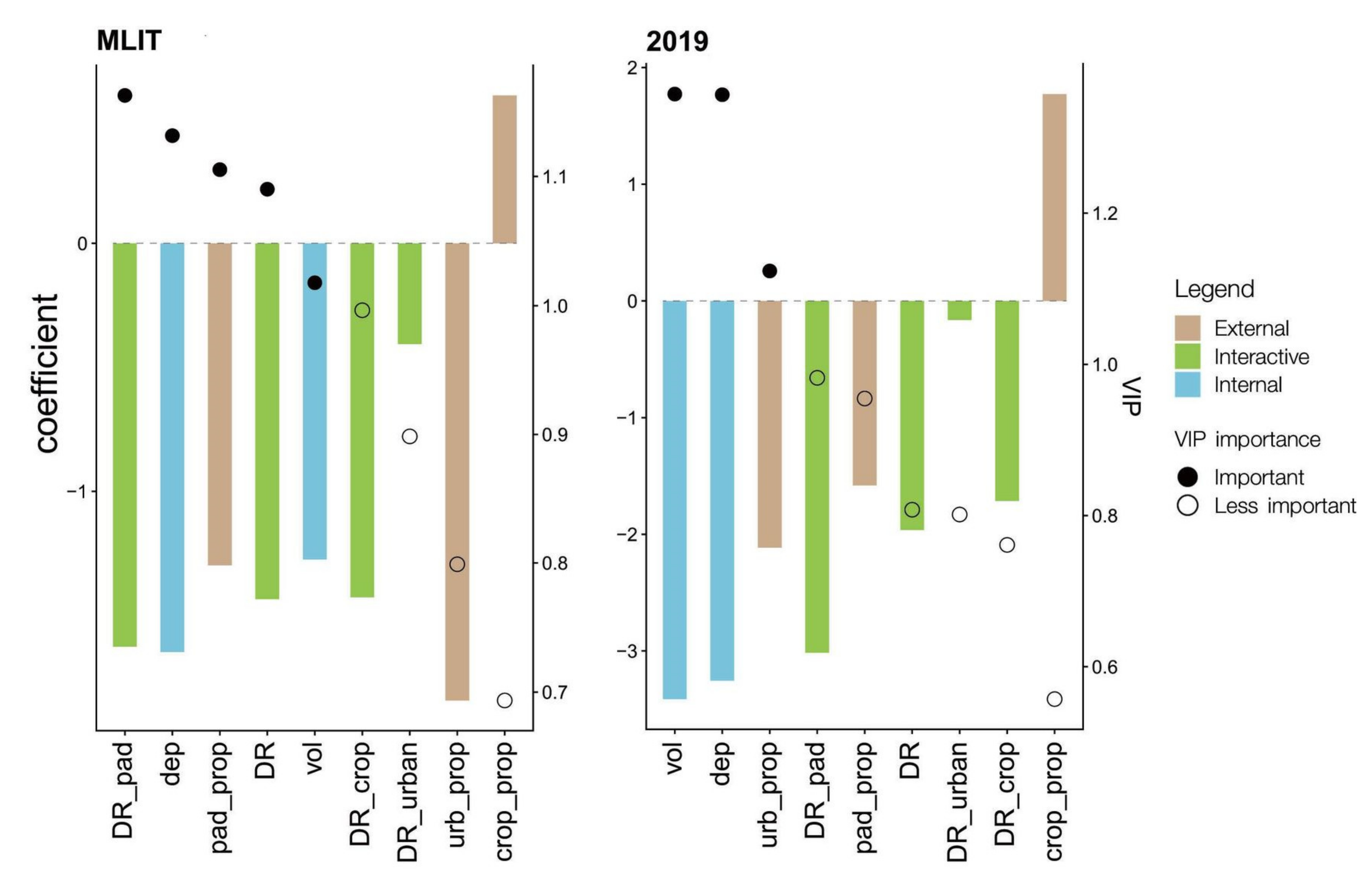
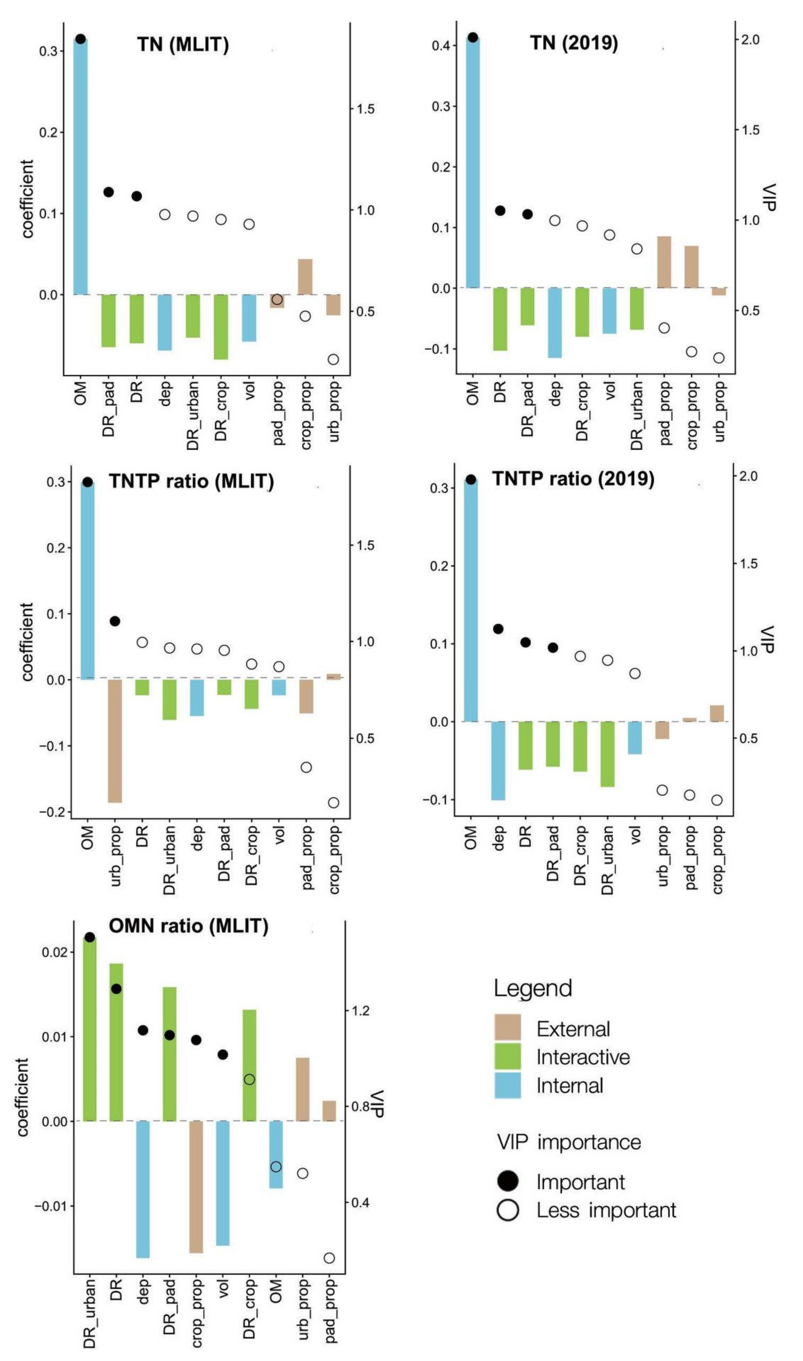
Explanatory variables were useful in predicting the variations of sediment properties for OM, TN, and TN to TP ratio in both years whereas the predictive power for OM to TN ratio was only observed in MLIT data (Table 3). For TP, no environmental variables were informative in predicting variations among FWBs. In both data sets, in general, the relative importance of variables did not differ substantially. For OM, morphometry variables were negative predictors together with several land use variables, indicating a higher amount of OM was observed in smaller, shallow FWBs (Figure 3). In 2019, two morphometry variables became two of the most important factors over the rest with the highest VIP values, indicating that morphometry controls on OM strengthened. At the same time, land use associated with human-activities had all negative contributions to the level of OM in both years. For TN and OM to TN ratio, OM was the most important factor in both years, indicating its strong controls of other sediment properties (Figure 4).
3.4. Factors Related to Temporal Variations in Sediment Properties
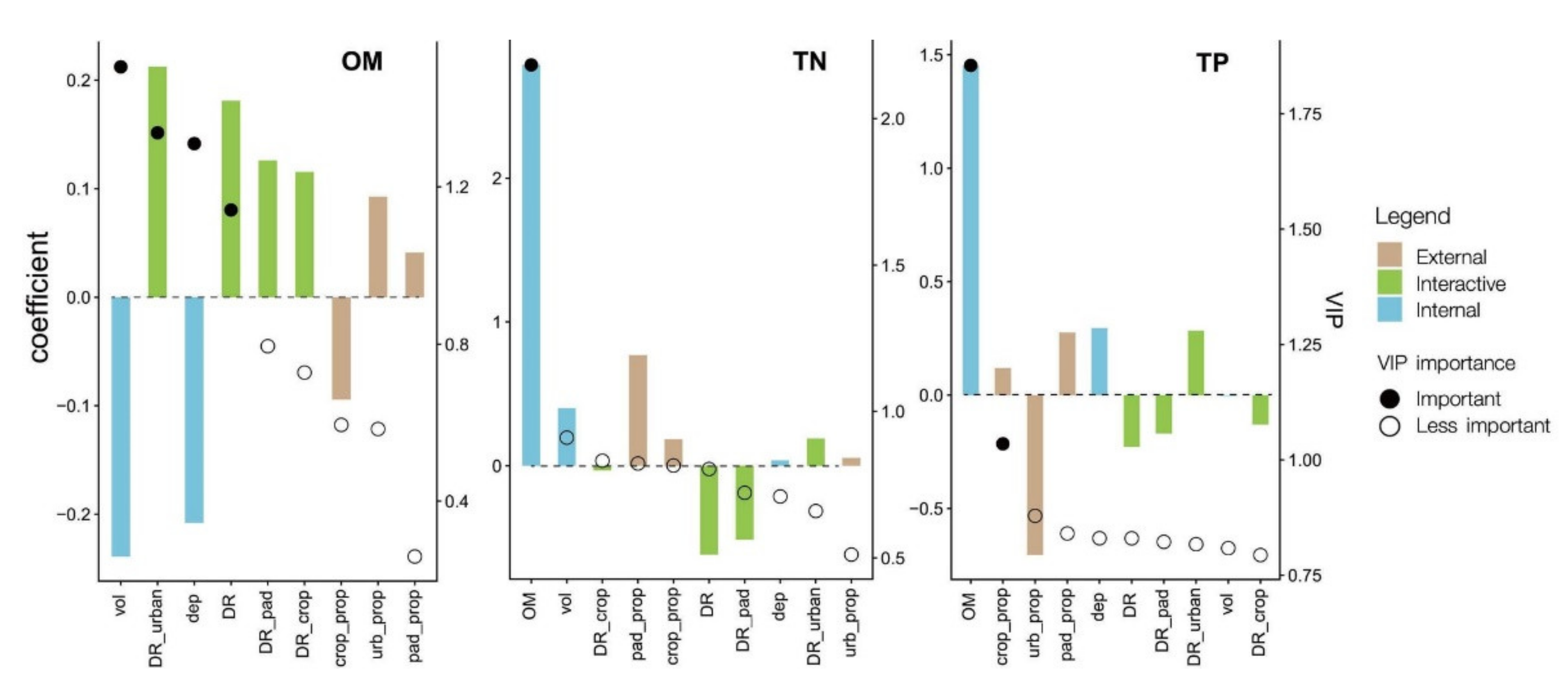
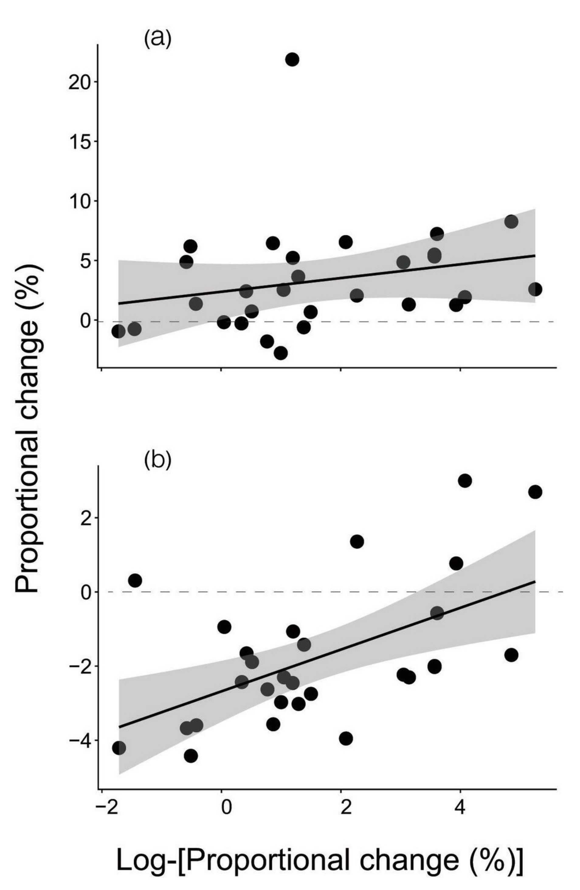
Explanatory variables were useful in predicting variations of property changes for OM, TN, and TP (Table 4). The change rate of OM was strongly explained by morphometry variables such as volume and depth with negative with both variables (Figure 5). Other important factors included drainage index related to urban land use with its positive contributions to the change in OM. These drainage indexes correlated with morphometry variables and thus they were not independent to each other (Table 4). The proportions of land use types in catchments were not selected as important factors. The changes in TN and TP were largely associated with the changes in OM, with both having positive relationships with TN and TP. Further analyses on the relationships among the change rates of OM and TN and TP showed that the increases in the change rate of OM was associated with the increase in the change rate of TN and TP (Figure 6). Change rate in TP was mostly negative; however, the rate remained relatively high at the level of zero change wherein OM was high. In contrast, the change rate in TN was mostly positive; however, the level of increase was minimal (up to several times) compared to the level of increase in OM (up to several tens of times).
3.5. Changes in OM in Relation to FWB Types
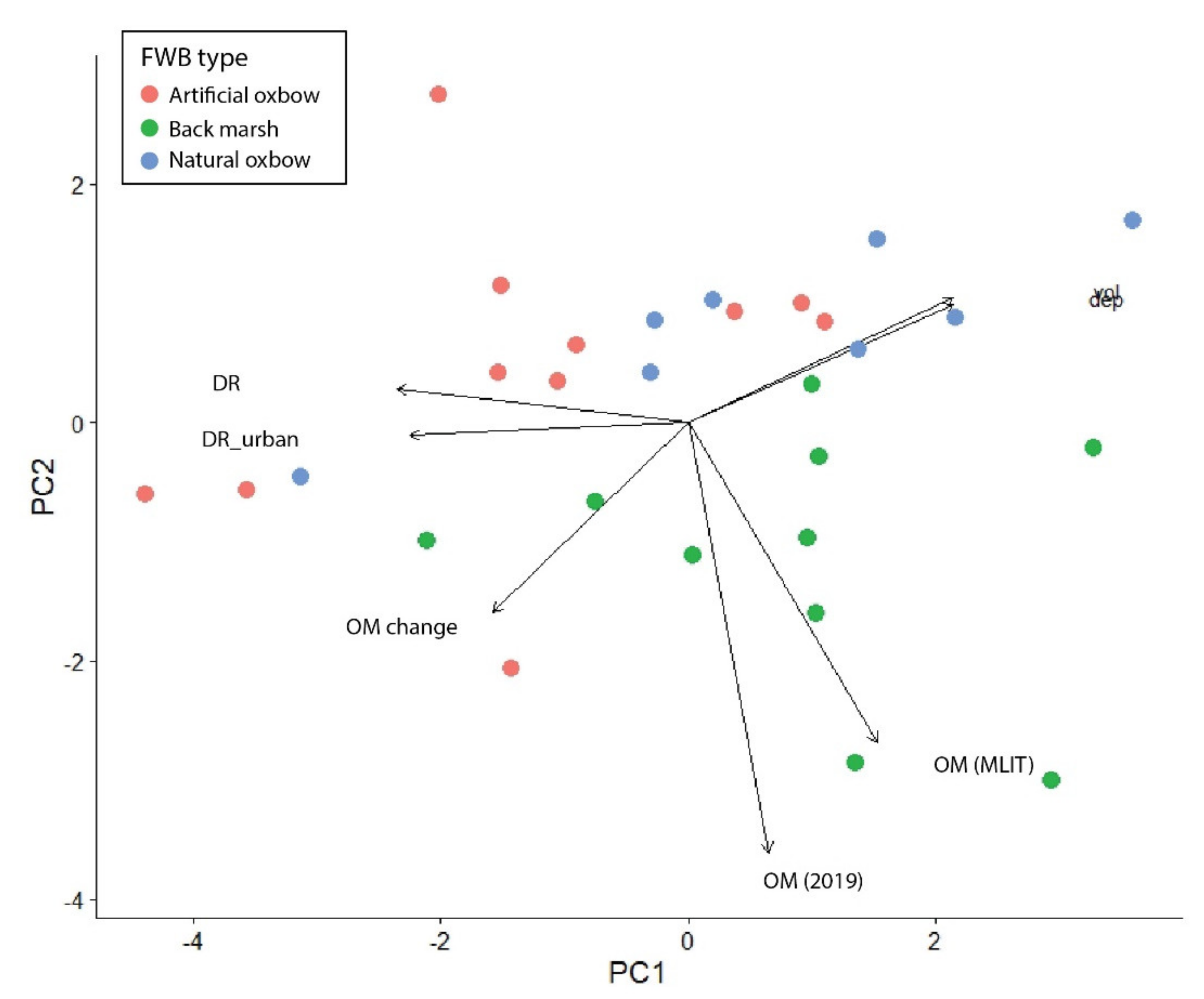
The change rate of OM, controlling factors of OM changes, and OM in both data sets, were included in PCA. Two PCA components together accounted for a variation of 77% of the original data (Figure 7). The axis PC-1 was largely associated with the internal properties of FWBs as well as human activities, and a part of the change rate of OM. The type most strongly associated with this axis were artificial and natural oxbow lakes, and especially those with shallow, and small morphometry experienced a high rate of increase of organic matter. Drainage indexes that are specific to urban land use were found to be also related to the gradient, supporting their correlation to the same component of OM in the PLS results (Table 4). In contrast, the axis PC-2 was associated with the spatial variation of OM in two data sets, showing that marsh FWBs were higher than two other types in OM content in both years. The loading arrow of OM in 2019 data was shifted in a clockwise direction relative to that in MLIT data, being closer to the PC-1 axis as well as the loading arrow of change rate of OM. This indicates that water bodies experiencing a high rate of change in OM have disproportionately increased its importance in characterizing FWBs along the gradient of OM. In addition, among those plotted in the third quadrant, which was characterized with high rate of OM change, artificial oxbow lakes were the most abundant (n = 3); the proportion in the third quadrant relative to all (27%) was also the highest for this water body type.
4. Discussion
Numerous previous studies of land-water interaction demonstrated the negative impacts of catchment activities on water quality of lentic ecosystems including floodplain waterbodies [20,22,26]. Similar results have become increasingly available for water bodies in Ishikari river floodplain in recent years [20]. Even though bottom sediment has the potential to mediate water quality via changes in quality in association with land use activities [38,57], it has been a seldom subject of focus in these previous studies. To our knowledge, the present study is the first report about simultaneous measurements of spatial variation of surface sediment quality, and their temporal changes in relation to their controlling environmental factors in floodplain. Our results support the contention that catchment properties as well as internal characteristics of waterbodies affect the trophic properties in lentic ecosystems. Our hypotheses and predictions about the negative influences of land use activities on sediment were largely unsupported, and the morphometry of water bodies were highlighted as the most important factors in explaining both spatial and temporal variations in sediment properties.
The spatial variations of sediment properties were related to several land-use related variables in a way opposite to our predictions [58]. Furthermore, this pattern was rather consistent across two survey years. Land use with extensive human activities such as agricultural fields are known as major sources of organic and inorganic matter transfer to the receiving water. This results in the eutrophication of water bodies, as the increasing intensity of land use activities contribute to more nutrient loading [57]. In our results, environmental variables associated with land use activities exhibited negative association with the proportion of organic matter, and nutrient contents such as nitrogen. This might be related to the fact that hydrological cycle, which was indirectly represented by drainage index and land surface areas of land use, played roles in cycling of matter and quality of sediment in water bodies rather than providing matter to be deposited within water bodies. For example, a high drainage ratio index can represent retention inefficiency of incoming matter as flushing and export of matter to further downstream sinks proliferate [27,28]. Moreover, it can reduce water retention time that can decelerate biogeochemical processes at the sediment–water interface [59]. The negative influences of morphometry on OM contents can be interpreted that shallow and smaller water bodies were characterized by a high OM content and associated nutrients. This can be explained by the relationship between morphometry and suitability for macrophyte growth [13]. In 2019, the importance of these internal processes on OM content became more apparent with other catchment influences having been weakened. Overall, there was no evidence of tight linkages between land use activity and sediment property for the study sites although high variations in morphometry among waterbodies might have masked the effects of land use on sediment properties.
There was little evidence that land use activities drove the changes in any properties of sediment over the period of about 15 years because none of the percentage land use types explained the sediment temporal changes. Overall, organic matter was associated with other properties such as nitrogen and phosphorus contents, suggesting it being a critical factor in understanding the mechanisms behind the patterns in sediment properties. Firstly, the OM and OM to TN ratio significantly increased from 2006 to 2019, which indicate that the accumulation of OM was stronger than the loss by mineralization or other processes. Together with the little changes in TN content, this result indicates that organic matter rich in C content has accumulated over time in the sediment, causing an increase of OM to TN ratio [34]. Because C and N are important energy source for microbial organisms that play important role on mineralization processes, the ratio between C and N in sediment could affect the intensity of mineralization. Normally, mineralization in sediment that contains low OM to TN ratio could be stronger than high OM to TN ratio due to the balance of available energy source [30,34]. Thus, reduced mineralization rates might have further accelerated the temporal increase of OM to TN ratio. The sources of deposited organic matter over the bed presumably included macrophytes and suspended algae. Algae typically contain relatively lower C in relation to nitrogen compared with macrophytes [60]. Therefore, it is unlikely that bottom sediments characterized with higher OM to N ratio in 2019 was caused by the accumulation of algae-derived organic matter over the time. Instead, it is inferred that macrophyte has contributed to the accumulation of C-rich sediment. This explanation is also supported by the finding that morphometry, which is known to affect habitat suitability of macrophytes [13], was among the most important controlling factors of the change rates. The effect direction was in line with the interpretation that the largest change was observed in shallow and smaller water bodies where macrophyte habitat suitability was relatively high. The average depth, which was also related to the areal extent of steeper-slope, showed a negative relationship with the spatial extent of macrophyte cover in FWBs [13]. Other studies also have demonstrated that depth was the main factor that controlled macrophyte distribution in lakes [29,61,62]. Drainage index, associated with urban land use had positive effects, implying that OM accumulation was also accelerated by external catchment activities. This might be caused by the increase of inorganic nutrients hence, the productivity of macrophyte, or supply of organics deposited to the water bodies. However, the correlations between variables related to land use and morphometry prevented us from concluding on the effects of this process. Morphometry plays a relevant role on soil properties since it controls water and sediment redistribution, affects the meteorological features relevant for temperature and moisture variation [63]. Moreover, topography influences the distribution of organic matter and soil nutrient, the rates of litter decomposition, the stability of OM, TP, and TN as results of transport and selectivity of geomorphic processes [64].
Only TP decreased over time, and this trend was similar to previous reports. Three explanations based on the past studies were plausible for the processes involved in this trend. First, the temporal decrease in TP has been attributed to the lower supply of P [8]. There were no changes in catchment activities in terms of spatial extent of land use that are potentially the source of P, a support of reduced TP supply of external source. Yet a general decrease in TP in the main channel of the Ishikari River has been reported for the period that overlapped with our study period [65]. There were no measurements of the influx of TP to the study FWBs, and thus it is impossible to rule out the possibility of this explanation. Second, the increase of OM might have depleted the dissolved oxygen in hypolimnetic water [31], and this possibly affected the change in P retention capacity of sediment. For example, the anoxic conditions in sediment can remobilize P from Fe-P fraction due to redox sensitive iron [38]. Moreover, P in Fe-P can be replaced by sulfur and become FeS in anoxic conditions [66]. This mechanism can be intensified in Fe rich sediment [38]. However, this explanation was inconsistent with a strong positive relationship between the change rate of TP and OM since a negative relationship is expected to support this explanation. The third explanation is based on the notion that the increase of OM content can cause an increase of cations in sediment since organic matter generally is characterized with high cation exchangeable capacity. Cations as Fe, Al, and Ca are elements that can fix P in sediment [8]. Thus, the change of OM contents can indirectly but positively affect the content of P in sediment. For example, Wang et al. [67] reported that the removal of OM from sediment showed a reduction in its P adsorption efficiency. Overall, our findings suggest that the processes in first and third explanations co-occurred during the study period. Furthermore, these TP related processes also provided weak evidence that land use activities have worsen the sediment quality.
Simultaneous plotting of spatial variations and temporal changes of sediment property allowed understanding of the changes in characteristics of surface sediment in relation to waterbody types. The rate of change in OM content appeared most evident in artificial oxbow lakes that were generally lower in the past. This change was driven by morphometry characteristics in relation to the different types of water bodies. Since a higher proportion of artificial oxbow lakes was relatively shallower and smaller compared to the other water body types, the change rate of OM was likely the most apparent. Negishi et al. [13] showed that natural oxbow and marsh were comparatively shallow, but their study did not include some of artificial oxbow lakes in the present study that were shallower and smaller in size. Another compelling explanation can be provided based on the formation history of artificial oxbow lakes. Most of these artificial disconnections were conducted via river works in the early 1900s [13,43], and thus the deposition of sediment with the lentic environment began in relatively recent years compared with the other water body types. Therefore, the succession in sediment properties from the former channel to the current condition may be more pronounced. Overall, FWBs in the study area are in the process of succession with the most apparent changes taking place in artificial oxbow lakes and is driven by their morphometric characteristics. Aging and succession of floodplain water bodies are known to occur under natural conditions and its pace can be accelerated by shallowing processes [29]. Yet we did not detect the decrease of water depth, further drastic changes in the internal properties of water bodies in terms of sediment quality may occur at the longer time scale.
In conclusion, our study demonstrated that the temporal change in surface sediment properties over decades was largely derived from morphometry and that land use in their catchment played a relatively minor role in those changes in Ishikari River FWBs. It was probable that the small and shallow FWBs provided suitable habitat for macrophytes that led to the accumulation of OM deposits to bottom sediment. This accumulation of OM was stronger than the removal processes resulting in an increase of OM and OM to TN ratio overtime. However, the change rate of OM differed among water bodies depending on their morphometry characteristics, thereby generating the spatial variation of sediment properties across the floodplain system. Interestingly, there was an indication that the increase of OM content in sediment might affect P adsorption efficiency in a complex way. Therefore, the role of OM level on P adsorption efficiency needs to be examined in the future. Our findings in the Ishikari River FWBs contrast with other studies since these reported stronger land-water interactions [20,26]. Sediment can act as internal source and has a potential to affect water quality in lake and/or reservoir systems [8,38,57]. The investigations into the mechanisms behind seemingly decoupled interactions between bottom sediment and water in the study FWBs would also provide critical implications to the management of FWBs.
Lastly, the foundation of high biodiversity in floodplains is the high turnover of the physio-chemical environment over a relatively small spatial extent [13,46]. In Ishikari River FWBs, a part of species turnover of aquatic species such as fish and mussels are known to be related to different types of water bodies that differ in depth, connectivity and morphometry [13,46]. Our findings suggest that artificial oxbow lakes are in the process of disproportionately more rapid succession of sediment properties. The consequence of these changes in the structure and function of biota and fauna are also an open and important topic to be addressed from the perspective of biodiversity conservation.
Supplementary Materials
The following are available online at https://www.mdpi.com/2073-4441/13/4/469/s1, Figure S1: Schematic diagram of FWB catchment characteristics, Figure S2: Boxplots showing the proportions of land use types (%) measured based on buffer strips, Figure S3: Boxplots showing the proportions of land use types (%) measured based on buffer strips and topographically defined catchments, Figure S4: Changes of sediment properties, Table S1: Results of log-likelihood tests examining the effects of observation year on the FWBs catchment characteristics, Table S2: Results of Spearman Rank’s correlations between landscape characteristics.
Author Contributions
Conceptualization, P.P. and J.N.N.; performed the field survey, P.P., J.N.N. and H.I.; laboratory analyses, P.P. and K.K.; FWBs catchment characteristics; J.N.N. and P.A.G.; statistical analyses, P.P. and J.N.N.; resources, J.N.N. and K.K.; writing—original draft preparation, P.P. and J.N.N.; writing—review and editing, J.N.N., H.I., P.A.G. and K.K. All authors have read and agreed to the published version of the manuscript.
Funding
This study is partly supported by the research fund for the Ishikari and Tokachi Rivers provided by the Ministry of Land, Infrastructure, Transport, and Tourism of Japan.
Institutional Review Board Statement
Not applicable.
Informed Consent Statement
Not applicable.
Data Availability Statement
The data supporting the findings of this study are available from the corresponding author upon reasonable request.
Acknowledgments
We are grateful for the support of the Ministry of Land, Infrastructure, Transport and Tourism (MLIT) who provided us with necessary data, and to the Ministry of Education, Culture, Sports, Science and Technology (MEXT) for the financial support as a MEXT scholar (P. Pongsivapai). We also deeply appreciate the assistance of Ryusuke Hatano and all members from Soil Science Laboratory of the Faculty of Agriculture, Hokkaido University for valuable suggestions and for providing facilities for chemical analysis.
Conflicts of Interest
The authors declare no conflict of interest.
References
- Wetzel, R.G. Limnology: Lake and River Ecosystems; Gulf Professional Publishing: San Diego, CA, USA, 2001. [Google Scholar]
- Forsberg, C. Importance of sediments in understanding nutrient cyclings in lakes. Hydrobiologia 1989, 176, 263–277. [Google Scholar] [CrossRef]
- Rydberg, J.; Lindborg, T.; Sohlenius, G.; Reuss, N.; Olsen, J.; Laudon, H. The importance of eolian input on lake-sediment geochemical composition in the dry proglacial landscape of western Greenland. Arctic Antarct. Alp. Res. 2016, 48, 93–109. [Google Scholar] [CrossRef] [Green Version]
- Smith, V.H. Eutrophication. In Encyclopedia of Inland Waters; Likens, G.E., Ed.; Elsevier: Oxford, UK, 2009; Volume 3, pp. 61–73. [Google Scholar]
- Fillos, J.; Swanson, W.R. The release rate of nutrients from river and lake sediments. J. Water Pollut. Control. Fed. 1975, 47, 1032–1042. [Google Scholar]
- Fisher, M.M.; Reddy, K.R.; James, R.T. Internal nutrient loads from sediments in a shallow, subtropical lake. Lake Reserv. Manag. 2005, 21, 338–349. [Google Scholar] [CrossRef]
- Lee, H.W.; Lee, Y.S.; Kim, J.; Lim, K.J.; Choi, J.H. Contribution of internal nutrients loading on the water quality of a reservoir. Water 2019, 11, 1409. [Google Scholar] [CrossRef] [Green Version]
- Søndergaard, M.; Jensen, J.P.; Jeppesen, E. Role of sediment and internal loading of phosphorus in shallow lakes. Hydrobiologia 2003, 506, 135–145. [Google Scholar] [CrossRef]
- Ribeiro, D.C.; Martins, G.; Nogueira, R.; Cruz, J.V.; Brito, A.G. Phosphorus fractionation in volcanic lake sediments (Azores-Portugal). Chemosphere 2008, 70, 1256–1263. [Google Scholar] [CrossRef] [Green Version]
- Mendonça, R.; Müller, R.A.; Tranvik, L.J.; Sobek, S.; Clow, D.; Verpoorter, C.; Raymond, P. Organic carbon burial in global lakes and reservoirs. Nat. Commun. 2017, 8, 1694. [Google Scholar] [CrossRef] [Green Version]
- Søndergaard, M.; Jeppesen, E.; Lauridsen, T.L.; Skov, C.; Van Nes, E.H.; Roijackers, R.; Lammens, E.; Portielje, R. Lake restoration: Successes, failures and long-term effects. J. Appl. Ecol. 2007, 44, 1095–1105. [Google Scholar] [CrossRef]
- Hickey, C.W.; Gibbs, M.M. Lake sediment phosphorus release management—Decision support and risk assessment framework support and risk assessment framework. N. Z. J. Mar. Freshwater Res. 2009, 43, 819–856. [Google Scholar] [CrossRef] [Green Version]
- Negishi, J.N.; Soga, M.; Ishiyama, N.; Suzuki, N.; Yuta, T.; Sueyoshi, M.; Yamazaki, C.; Koizumi, I.; Mizugaki, S.; Hayashida, K.; et al. Geomorphic legacy controls macrophyte distribution within and across disconnected floodplain lakes. Freshw. Biol. 2014, 59, 942–954. [Google Scholar] [CrossRef]
- Ward, J.V.; Tockner, K.; Schiemer, F. Biodiversity of floodplain river ecosystems: Ecotones and connectivity. Regul. Rivers Res. Manag. 1999, 15, 125–139. [Google Scholar] [CrossRef]
- Hauer, F.R.; Locke, H.; Dreitz, V.J.; Hebblewhite, M.; Lowe, W.H.; Muhlfeld, C.C.; Nelson, C.R.; Proctor, M.F.; Rood, S.B. Gravel-bed river floodplains are the ecological nexus of glaciated mountain landscapes. Sci. Adv. 2016, 2, e1600026. [Google Scholar] [CrossRef] [Green Version]
- Paira, A.R.; Drago, E.C. Origin, Evolution, and Types of Floodplain Water Bodies. In The Middle Paraná River: Limnology of a Subtropical Wetland; Iriondo, M.H., Paggi, J.C., Parma, M.J., Eds.; Springer: Berlin/Heidelberg, Germany, 2007; pp. 53–81. [Google Scholar]
- Rivetti, C.; López-Perea, J.J.; Laguna, C.; Piña, B.; Mateo, R.; Eljarrat, E.; Barceló, D.; Barata, C. Integrated environmental risk assessment of chemical pollution in a Mediterranean floodplain by combining chemical and biological methods. Sci. Total Environ. 2017, 583, 248–256. [Google Scholar] [CrossRef]
- Tockner, K.; Stanford, J.A. Riverine flood plains: Present state and future trends. Environ. Conserv. 2002, 29, 308–330. [Google Scholar] [CrossRef] [Green Version]
- Petry, P.; Bayley, P.B.; Markle, D.F. Relationships between fish assemblages, macrophytes and environmental gradients in the Amazon River floodplain. J. Fish. Biol. 2003, 63, 547–579. [Google Scholar] [CrossRef]
- Kizuka, T.; Yamada, H.; Yazawa, M.; Chung, H.H. Effects of agricultural land use on water chemistry of mire pools in the Ishikari Peatland, northern Japan. Landsc. Ecol. Eng. 2008, 4, 27–37. [Google Scholar] [CrossRef]
- Negishi, J.N.; Sagawa, S.; Kayaba, Y.; Sanada, S.; Kume, M.; Miyashita, T. Mussel responses to flood pulse frequency: The importance of local habitat. Freshw. Biol. 2012, 57, 1500–1511. [Google Scholar] [CrossRef]
- Houlahan, J.E.; Findlay, C.S. Estimating the ‘critical’ distance at which adjacent land-use degrades wetland water and sediment quality. Landsc. Ecol. 2004, 19, 677–690. [Google Scholar] [CrossRef]
- Wilson, C.; Weng, Q. Assessing surface water quality and its relation with urban land cover changes in the Lake Calumet Area, Greater Chicago. Environ. Manag. 2010, 45, 1096–1111. [Google Scholar] [CrossRef] [PubMed]
- Coulter, C.B.; Kolka, R.K.; Thompson, J.A. Water quality in agricultural, urban, and mixed land use watersheds. J. Am. Water Resour. Assoc. 2004, 40, 1593–1601. [Google Scholar] [CrossRef]
- Walker, W.J.; McNutt, R.P.; Maslanka, C.K. The potential contribution of urban runoff to surface sediments of the Passaic River: Sources and chemical characteristics. Chemosphere 1999, 38, 363–377. [Google Scholar] [CrossRef]
- Ahn, Y.S.; Nakamura, F.; Kizuka, T.; Yugo, N. Elevated sedimentation in lake records linked to agricultural activities in the Ishikari River floodplain, northern Japan. Earth Surf. Process. Landf. 2009, 34, 1650–1660. [Google Scholar] [CrossRef]
- Sobek, S.; Tranvik, L.J.; Prairie, Y.T.; Kortelainen, P.; Cole, J.J. Patterns and regulation of dissolved organic carbon: An analysis of 7500 widely distributed lakes. Limnol. Oceanogr. 2007, 52, 1208–1219. [Google Scholar] [CrossRef] [Green Version]
- Cremona, F.; Laas, A.; Hanson, P.C.; Sepp, M.; Nõges, P.; Nõges, T. Drainage ratio as a strong predictor of allochthonous carbon budget in hemiboreal lakes. Ecosystems 2018, 22, 805–817. [Google Scholar] [CrossRef]
- Lawniczak-Malińska, A.; Ptak, M.; Celewicz, S.; Choiński, A. Impact of lake morphology and shallowing on the rate of overgrowth in hard-water eutrophic lakes. Water 2018, 10, 1827. [Google Scholar] [CrossRef] [Green Version]
- Gälman, V.; Rydberg, J.; de-Luna, S.S.; Bindler, R.; Renberg, I. Carbon and nitrogen loss rates during aging of lake sediment: Changes over 27 years studied in varved lake sediment. Limnol. Oceanogr. 2008, 53, 1076–1082. [Google Scholar] [CrossRef] [Green Version]
- Den Heyer, C.; Kalff, J. Organic matter mineralization rates in sediments: A within- and among-lake study. Limnol. Oceanogr. 1998, 43, 695–705. [Google Scholar] [CrossRef]
- Gale, P.M.; Reddy, K.R.; Graetz, D.A. Mineralization of sediment organic matter under anoxic conditions. J. Environ. Qual. 1992, 21, 394–400. [Google Scholar] [CrossRef] [Green Version]
- Tang, F.; Huang, T.; Fan, R.; Luo, D.; Yang, H.; Huang, C. Temporal variation in sediment C, N, and P stoichiometry in a plateau lake during sediment burial. J. Soils Sediments 2020, 20, 1706–1718. [Google Scholar] [CrossRef]
- Twichell, S.C.; Meyers, P.A.; Diester-Haass, L. Significance of high C/N ratios in organic-carbon-rich Neogene sediments under the Benguela Current upwelling system. Org. Geochem. 2002, 33, 715–722. [Google Scholar] [CrossRef]
- Geurts, J.J.M.; Smolders, A.J.P.; Banach, A.M.; van de Graaf, J.P.M.; Roelofs, J.G.M.; Lamers, L.P.M. The interaction between decomposition, net N and P mineralization and their mobilization to the surface water in fens. Water Res. 2010, 44, 3487–3495. [Google Scholar] [CrossRef] [PubMed]
- Gudasz, C.; Bastviken, D.; Steger, K.; Premke, K.; Sobek, S.; Tranvik, L.J. Temperature-controlled organic carbon mineralization in lake sediments. Nature 2010, 466, 478–481. [Google Scholar] [CrossRef]
- Lalonde, K.; Mucci, A.; Ouellet, A.; Gélinas, Y. Preservation of organic matter in sediments promoted by iron. Nature 2012, 483, 198–200. [Google Scholar] [CrossRef] [Green Version]
- Hayakawa, A.; Ikeda, S.; Tsushima, R.; Ishikawa, Y.; Hidaka, S. Spatial and temporal variations in nutrients in water and riverbed sediments at the mouths of rivers that enter Lake Hachiro, a shallow eutrophic lake in Japan. Catena 2015, 133, 486–494. [Google Scholar] [CrossRef] [Green Version]
- Wang, S.; Jin, X.; Zhao, H.; Wu, F. Phosphorus release characteristics of different trophic lake sediments under simulative disturbing conditions. J. Hazard. Mater. 2009, 161, 1551–1559. [Google Scholar] [CrossRef]
- Kaushal, S.; Binford, M.W. Relationship between C:N ratios of lake sediments, organic matter sources, and historical deforestation in Lake Pleasant, Massachusetts, USA. J. Paleolimnol. 1999, 22, 439–442. [Google Scholar] [CrossRef]
- Ishii, Y.; Hori, K.; Momohara, A. Middle to late Holocene flood activity estimated from loss on ignition of peat in the Ishikari lowland, northern Japan. Glob. Planet. Chang. 2017, 153, 1–15. [Google Scholar] [CrossRef]
- Soga, M.; Ishiyama, N.; Sueyoshi, M.; Yamaura, Y.; Hayashida, K.; Koizumi, I.; Negishi, J.N. Interaction between patch area and shape: Lakes with different formation processes have contrasting area and shape effects on macrophyte diversity. Landsc. Ecol. Eng. 2014, 10, 55–64. [Google Scholar] [CrossRef] [Green Version]
- Hayashida, K.; Hirayama, A.; Ueda, H. Changes in fish fauna in oxbow lakes on the Ishikari river and the influence of invasive fish species. Annu. J. Hydraul. Eng. 2010, 54, 1261–1266. (In Japanese) [Google Scholar]
- Kusa, D.; Yamamoto, T.; Inoue, T.; Nagasawa, T. Evaluation of oxbow lakes and circulating irrigation in the Ishikari River basin, Japan. Int. J. Environ. Rural Dev. 2014, 5, 65–71. [Google Scholar]
- Ishiyama, N.; Miura, K.; Yamanaka, S.; Negishi, J.N.; Nakamura, F. Contribution of small isolated habitats in creating refuges from biological invasions along a geomorphological gradient of floodplain waterbodies. J. Appl. Ecol. 2019, 57, 548–558. [Google Scholar] [CrossRef]
- Izumi, H.; Negishi, J.N.; Miura, K.; Ito, D.; Pongsivapai, P. Distribution and life-history traits of Unionoid mussels in floodplain waterbodies of the Ishikari River. Ecol. Civ. Eng. 2020, 23, 1–20. (In Japanese) [Google Scholar] [CrossRef]
- MLIT A Comprehensive Plan for Nature Restoration of Lowlands of the Ishikari River. Available online: https://www.hkd.mlit.go.jp/sp/kasen_keikaku/kluhh40000002hwd-att/kluhh4000000cx8y.pdf (accessed on 9 November 2020). (In Japanese)
- Jha, P.K.; Minagawa, M. Assessment of denitrification process in lower Ishikari river system, Japan. Chemosphere 2013, 93, 1726–1733. [Google Scholar] [CrossRef]
- Ishii, Y.; Hori, K. Formation and infilling of oxbow lakes in the Ishikari lowland, northern Japan. Quat. Int. 2016, 397, 136–146. [Google Scholar] [CrossRef]
- Zhu, M. Aquatic Food-Web Structure in Floodplain Waterbodies in Relation to Nutrient Pollution, Ecosystem Size, and Invasive Species. Master’s Thesis, Hokkaido University, Sapporo, Japan, 2017. [Google Scholar]
- Nakatani, N.; Otomichi, M.; Yoshida, O.; Ushiyama, K. Evaluation of the degree of water pollution and estimation of phosphorus loads from migrating birds in Lake Miyajimanuma, Hokkaido. Wetl. Res. 2014, 5, 15–23. (In Japanese) [Google Scholar] [CrossRef]
- Nasir, A.; Lukman, M.; Tuwo, A.; Hatta, M.; Tambaru, R. Nurfadilah the use of C/N ratio in assessing the influence of land-based material in coastal water of South Sulawesi and Spermonde Archipelago, Indonesia. Front. Mar. Sci. 2016, 3, 266. [Google Scholar] [CrossRef] [Green Version]
- Novikmec, M.; Hamerlík, L.; Kočický, D.; Hrivnák, R.; Kochjarová, J.; Oťaheľová, H.; Pal’ove-Balang, P.; Svitok, M. Ponds and their catchments: Size relationships and influence of land use across multiple spatial scales. Hydrobiologia 2016, 774, 155–166. [Google Scholar] [CrossRef]
- Wold, S.; Sjöström, M.; Eriksson, L. PLS-regression: A basic tool of chemometrics. Chemom. Intell. Lab. Syst. 2001, 58, 109–130. [Google Scholar] [CrossRef]
- R Core Team. R: A Language and Environment for Statistical Computing; R Core Team: Vienna, Austria, 2018. [Google Scholar]
- Larson, J.H.; Staples, D.F.; Maki, R.P.; Vallazza, J.M.; Knights, B.C.; Peterson, K.E. Do water level fluctuations influence production of walleye and yellow perch young-of-the-year in large northern lakes? N. Am. J. Fish. Manag. 2016, 36, 1425–1436. [Google Scholar] [CrossRef]
- Carter, L.D.; Dzialowski, A.R. Predicting sediment phosphorus release rates using landuse and water-quality data. Freshw. Sci. 2012, 31, 1214–1222. [Google Scholar] [CrossRef]
- Von Lützow, M.; Kögel-Knabner, I.; Ekschmitt, K.; Matzner, E.; Guggenberger, G.; Marschner, B.; Flessa, H. Stabilization of organic matter in temperate soils: Mechanisms and their relevance under different soil conditions—A review. Eur. J. Soil Sci. 2006, 57, 426–445. [Google Scholar] [CrossRef]
- Gu, C.; Hornberger, G.M.; Mills, A.L.; Herman, J.S.; Flewelling, S.A. Nitrate reduction in streambed sediments: Effects of flow and biogeochemical kinetics. Water Resour. Res. 2007, 43, W12413. [Google Scholar] [CrossRef] [Green Version]
- Liu, S.; Zhao, T.; Zhu, Y.; Qu, X.; He, Z.; Giesy, J.P.; Meng, W. Molecular characterization of macrophyte-derived dissolved organic matters and their implications for lakes. Sci. Total Environ. 2018, 616–617, 602–613. [Google Scholar] [CrossRef] [PubMed]
- Duarte, C.M.; Kalff, J. Patterns in the submerged macrophyte biomass of lakes and the importance of the scale of analysis in the interpretation. Can. J. Fish. Aquat. Sci. 1990, 47, 357–363. [Google Scholar] [CrossRef]
- Ye, B.; Chu, Z.; Wu, A.; Hou, Z.; Wang, S. Optimum water depth ranges of dominant submersed macrophytes in a natural freshwater lake. PLoS ONE 2018, 13, e0193176. [Google Scholar] [CrossRef] [Green Version]
- Lucà, F.; Buttafuoco, G.; Terranova, O. GIS and Soil. In Comprehensive Geographic Information Systems; Huang, B., Ed.; Elsevier: Oxford, UK, 2018; Volume 2, pp. 37–50. ISBN 9780128046609. [Google Scholar] [CrossRef]
- Conforti, M.; Lucà, F.; Scarciglia, F.; Matteucci, G.; Buttafuoco, G. Soil carbon stock in relation to soil properties and landscape position in a forest ecosystem of southern Italy (Calabria region). Catena 2016, 144, 23–33. [Google Scholar] [CrossRef]
- Duan, W.; Takara, K.; He, B.; Luo, P.; Nover, D.; Yamashiki, Y. Spatial and temporal trends in estimates of nutrient and suspended sediment loads in the Ishikari River, Japan, 1985 to 2010. Sci. Total Environ. 2013, 461–462, 499–508. [Google Scholar] [CrossRef]
- Ribeiro, D.C.; Martins, G.; Nogueira, R.; Brito, A.G. Mineral cycling and pH gradient related with biological activity under transient anoxic-oxic conditions: Effect on P mobility in volcanic lake sediments. Environ. Sci. Technol. 2014, 48, 9205–9210. [Google Scholar] [CrossRef] [Green Version]
- Wang, Y.; Shen, Z.; Niu, J.; Liu, R. Adsorption of phosphorus on sediments from the Three-Gorges Reservoir (China) and the relation with sediment compositions. J. Hazard. Mater. 2009, 162, 92–98. [Google Scholar] [CrossRef]
Figure 1.
(a) The main channel (shown within the shaded area) of the Ishikari River in Hokkaido, northern Japan. (b) Locations of three types of floodplain water bodies: gray, black and open circles indicate artificially formed oxbow lakes (A), naturally formed oxbow lakes (N) and marsh lakes (M), respectively. Identification labels were attached to each of the circles; see Table 1 for more details. A star denotes a weather station of the Japan Meteorological Agency where data of precipitation and temperature were obtained. Bird-view pictures represent two example water bodies.

Figure 2.
(a) OM (%); (b) TN (mg/g); (c) TP (mg/g); (d) OM to TN ration; (e) TN to TP ratio; Boxplot showing changes of sediment characteristics between two types of data set. MLIT refers to those collected by the Ministry of land, infrastructure, transport and tourism (MLIT) between 2003–2006 while 2019 was collected in this study in 2019. Data points from the same water bodies were connected by lines for clarity. Asterisks denote statistically significant differences as a result of GLMMs at p < 0.001.

Figure 3.
Partial least squares (PLS) regression output for the organic matter content (%) in MLIT data and 2019 data. Variables are listed with regression coefficients in descending variable importance to the projection (VIP) index order. VIP > 1 is considered important (filled circles) and VIP < 1 is less important (open circles). Abbreviations: dep for depth; vol for volume; DR for drainage index; DR_pad, DR_crop and DR_urban for drainage index based on the total area of paddy fields, crop fields, urban areas, respectively; pad_prop, crop_prop, and urb_prop for the proportion of paddy fields, crop fields, and urban areas, respectively.

Figure 4.
Partial least squares regression (PLS) output for total nitrogen (TN), nitrogen to phosphorus (TNTP ratio) ratio and organic matter to nitrogen (OMN ratio) ratio in MLIT data and 2019 data. Variables are listed with regression coefficients in descending VIP (variable importance to the projection) index order. VIP > 1 is considered important (filled circles) and VIP < 1 is less important (open circles). For abbreviations, OM for organic matter and see Figure 3.

Figure 5.
Partial least squares regression (PLS) output for the change rate (%) of organic matter (OM), total nitrogen (TN), and total phosphorus (TP). Variables are listed with regression coefficients in descending VIP (variable importance to the projection) index order. VIP > 1 is considered important (filled circles) and VIP < 1 is less important (open circles). For abbreviations, see Figure 3.

Figure 6.
Relationships between the change rate of organic matter and total nitrogen (a) and between the change rate of organic matter and total phosphorus (b). In both panes, the change rate of organic matter is plotted on a horizontal axis. Regression line and 95% confidence intervals were also shown.

Figure 7.
The correlations between temporal and spatial patterns in organic matter contents of sediment and their controlling variables. Three different types of floodplain water body are also shown. Out of the overall variation of organic matter content, 55% is displayed on the horizontal axis (PC1) and another 22% of the vertical axis.


Table 1.
General characteristics of floodplain waterbodies (FWBs) in the Ishikari River. The names of FWBs are provided as codes whose location is shown in Figure 1. Catchment area was estimated by including 200 m buffer area around the water edge, 100 m buffer areas on both sides of agricultural channels that drained through the areas not defined by topography, and other all topographically-defined catchment contributing to FWBs (see the text in more details about estimation method). Total nitrogen (TN) and total phosphorus (TP) of surface water were showed in mean values of data from MLIT and survey in 2019 (water quality data was collected in summer and autumn in both data sets) as an index of trophic status.
| FWB ID | FWB Type | Surface Area (×103 m2) | Depth (m) | Volume (×103 m3) | Catchment Area (×103 m2) | Drainage Index (m−1) | TN (mg/L) | TP (mg/L) | Trophic State | MLIT Data Year |
|---|---|---|---|---|---|---|---|---|---|---|
| A1 | Artificial | 37.63 | 0.22 | 8.28 | 6002.25 | 724.91 | 2.328 | 0.149 | Hypertrophic | 2005 |
| A2 | Artificial | 45.87 | 1.94 | 88.99 | 1154.16 | 12.97 | 1.931 | 0.086 | Hypertrophic | 2005 |
| A3 | Artificial | 127.40 | 0.34 | 43.74 | 1163.23 | 26.59 | 5.223 | 0.630 | Hypertrophic | 2005 |
| A4 | Artificial | 25.26 | 0.28 | 7.07 | 2679.08 | 378.94 | 1.831 | 0.159 | Hypertrophic | 2005 |
| A5 | Artificial | 50.17 | 1.24 | 62.21 | 347.91 | 5.59 | 0.558 | 0.061 | Eutrophic | 2005 |
| A6 | Artificial | 78.43 | 3.26 | 255.68 | 9013.87 | 35.25 | 1.177 | 0.100 | Eutrophic | 2005 |
| A7 | Artificial | 111.10 | 0.42 | 46.66 | 14,481.57 | 310.36 | 1.236 | 0.075 | Eutrophic | 2004 |
| A8 | Artificial | 56.91 | 0.92 | 52.17 | 21,954.90 | 420.83 | 2.343 | 0.171 | Hypertrophic | 2005 |
| A9 | Artificial | 38.83 | 0.40 | 15.53 | 1646.98 | 106.05 | 1.374 | 0.166 | Hypertrophic | 2005 |
| A10 | Artificial | 403.90 | 0.30 | 121.17 | 12,825.36 | 105.85 | 3.191 | 0.299 | Hypertrophic | 2005 |
| A11 | Artificial | 86.18 | 0.56 | 48.26 | 1201.61 | 24.90 | 0.708 | 0.057 | Eutrophic | 2005 |
| M1 | Marsh | 11.69 | 0.40 | 4.68 | 247.87 | 52.96 | 2.534 | 0.081 | Eutrophic | 2006 |
| M2 | Marsh | 175.30 | 0.77 | 134.40 | 2722.16 | 20.25 | 1.752 | 0.169 | Hypertrophic | 2006 |
| M3 | Marsh | 50.83 | 0.37 | 18.64 | 814.02 | 43.67 | 2.398 | 0.159 | Hypertrophic | 2006 |
| M4 | Marsh | 67.74 | 0.80 | 54.19 | 913.77 | 16.86 | 1.158 | 0.096 | Eutrophic | 2006 |
| M5 | Marsh | 21.46 | 1.34 | 28.76 | 810.57 | 28.18 | 2.565 | 0.087 | Eutrophic | 2006 |
| M6 | Marsh | 96.76 | 1.60 | 154.82 | 337.92 | 2.18 | 1.126 | 0.069 | Eutrophic | 2006 |
| M7 | Marsh | 26.57 | 1.30 | 34.54 | 498.69 | 14.44 | 1.417 | 0.087 | Eutrophic | 2006 |
| M8 | Marsh | 283.30 | 0.35 | 99.16 | 1029.21 | 10.38 | 7.880 | 0.655 | Hypertrophic | 2006 |
| M9 | Marsh | 64.21 | 1.32 | 84.54 | 748.50 | 8.85 | 2.381 | 0.136 | Hypertrophic | 2006 |
| M10 | Marsh | 105.10 | 3.04 | 319.50 | 1044.34 | 3.27 | 0.962 | 0.057 | Eutrophic | 2006 |
| N1 | Natural | 241.10 | 0.40 | 96.44 | 5644.15 | 58.52 | 0.942 | 0.204 | Hypertrophic | 2003 |
| N2 | Natural | 112.10 | 0.16 | 17.71 | 12,542.11 | 708.19 | 0.601 | 0.053 | Eutrophic | 2004 |
| N3 | Natural | 142.40 | 1.68 | 239.23 | 888.28 | 3.71 | 1.686 | 0.081 | Eutrophic | 2004 |
| N4 | Natural | 118.30 | 0.62 | 73.35 | 1779.48 | 24.26 | 0.705 | 0.070 | Eutrophic | 2004 |
| N5 | Natural | 88.71 | 6.67 | 591.70 | 629.52 | 1.06 | 0.543 | 0.043 | Eutrophic | 2005 |
| N6 | Natural | 112.70 | 3.12 | 351.62 | 865.02 | 2.46 | 1.227 | 0.111 | Hypertrophic | 2004 |
| N7 | Natural | 73.63 | 2.40 | 176.71 | 1079.20 | 6.11 | 1.083 | 0.070 | Eutrophic | 2005 |
| N8 | Natural | 129.50 | 0.88 | 113.96 | 2955.53 | 25.93 | 1.213 | 0.108 | Hypertrophic | 2005 |
Table 2.
Results of Generalized Linear Mixed Models (GLMM) testing the effects of data type (data obtained from MLIT or data obtained in 2019) on the sediment characteristics. Statistical significance based on results of Z statistics are shown. Abbreviations: OM is organic matter content (%); TN is total nitrogen (mg/g); TP is total phosphorus (mg/g); AIC is Akaike’s Information Criteria; SE is standard.
| Variables | Log-likelihood | AIC | Estimates | SE | Z | p |
|---|---|---|---|---|---|---|
| OM | −162.9 | 333.7 | 2.4580 | 0.5990 | 4.10 | <0.001 |
| TN | −126.0 | 260.0 | 0.1051 | 0.3840 | 0.27 | 0.78 |
| TP | −38.9 | 85.7 | −0.4058 | 0.0948 | −4.28 | <0.001 |
| OM to TN | −12.3 | 32.6 | 0.2179 | 0.0712 | 3.06 | <0.01 |
| TN to TP | −36.6 | 81.3 | 0.3027 | 0.0708 | 4.28 | <0.001 |
Table 3.
Output of partial least square (PLS) regression relating predictor variables to four response variables of sediment characteristics in floodplain water bodies. “MLIT” refers to data collected by MLIT whereas data collected in 2019 was shown as “2019”. Loading with absolute values less than 0.1 are not shown (–). Components (C) for organic matter to nitrogen (OMN) ratio in data collected in 2019 is not shown because no acceptable PLS model was developed. “NA” denote not applicable. Other abbreviations: DR for drainage index; DR_pad, DR_crop and DR_urban for drainage index based on the total area of paddy fields, crop fields, urban areas, respectively; %paddy, %crop, and %urban for the proportion of paddy fields, crop fields, and urban areas.
| OM (3, 4) | TN (3, 3) | TN to TP (2, 2) | OMN (1) | ||||||||||||||||
|---|---|---|---|---|---|---|---|---|---|---|---|---|---|---|---|---|---|---|---|
| Cumulative % of variance explained (response variables) | 54.42 | 49.29 | 84.39 | 76.80 | 66.25 | 48.28 | 19.11 | ||||||||||||
| Cumulative % of variance explained (predictor variables) | 76.52 | 86.48 | 75.88 | 70.24 | 60.75 | 57.86 | 45.56 | ||||||||||||
| Component loadings | |||||||||||||||||||
| MLIT | 2019 | MLIT | 2019 | MLIT | 2019 | MLIT | |||||||||||||
| Variables | C1 | C2 | C3 | C1 | C2 | C3 | C4 | C1 | C2 | C3 | C1 | C2 | C3 | C1 | C2 | C1 | C2 | C1 | |
| OM | NA | NA | NA | NA | NA | NA | NA | 0.33 | 0.62 | 0.12 | 0.37 | 0.54 | 0.36 | 0.48 | 0.33 | 0.62 | −0.27 | ||
| Depth | 0.40 | −0.38 | −0.24 | 0.44 | −0.55 | −0.22 | 0.11 | 0.36 | −0.46 | −0.13 | 0.36 | −0.50 | 0.37 | −0.42 | 0.37 | −0.51 | −0.39 | ||
| Volume | 0.39 | −0.30 | −0.31 | 0.44 | −0.54 | −0.20 | 0.17 | 0.35 | −0.41 | −0.20 | 0.35 | −0.50 | 0.37 | −0.35 | 0.36 | −0.48 | −0.38 | ||
| DR | −0.46 | 0.19 | −0.12 | −0.56 | 0.20 | −0.44 | 0.18 | −0.10 | −0.53 | 0.25 | −0.45 | 0.30 | −0.51 | 0.24 | 0.44 | ||||
| %paddy | −0.12 | −0.84 | 0.49 | −0.19 | −0.56 | 0.45 | −0.21 | −0.11 | −0.35 | 0.70 | 0.70 | −0.11 | −0.17 | ||||||
| %crop | 0.10 | 0.52 | −0.60 | −0.33 | 0.93 | 0.27 | −0.57 | 0.18 | −0.12 | ||||||||||
| %urban | −0.27 | −0.32 | 0.57 | −0.69 | −0.27 | 0.15 | −0.63 | −0.16 | −0.50 | ||||||||||
| DR_pad | −0.45 | −0.15 | −0.58 | 0.13 | −0.44 | 0.14 | −0.52 | 0.20 | 0.29 | −0.43 | 0.25 | −0.49 | 0.19 | 0.42 | |||||
| DR_crop | −0.39 | 0.31 | −0.47 | −0.48 | 0.16 | −0.28 | 0.47 | −0.39 | 0.21 | −0.38 | −0.48 | 0.17 | −0.40 | 0.23 | −0.47 | 0.15 | 0.37 | ||
| DR_urban | −0.42 | 0.17 | −0.25 | −0.43 | 0.46 | −0.45 | −0.41 | 0.24 | −0.17 | −0.43 | 0.29 | −0.37 | −0.43 | 0.16 | −0.43 | 0.22 | 0.42 | ||
Table 4.
Output of partial least square regression (PLS) relating predictor variables to change rates of three response variables of sediment characteristics (OM: organic matter content; TN: total nitrogen; TP: total phosphorus) in floodplain water bodies. Loading with absolute values less than 0.1 are not shown. For more information on abbreviations and symbols, refer to Table 3.
| OM (1) | TN (3) | TP (3) | |||||
|---|---|---|---|---|---|---|---|
| Cumulative % of variance explained (response variables) | 28.74 | 49.50 | 52.32 | ||||
| Cumulative % of variance explained (predictor variables) | 50.87 | 70.69 | 72.70 | ||||
| Component loadings | |||||||
| Variables | C1 | C1 | C2 | C3 | C1 | C2 | C3 |
| OM | NA | 0.72 | 0.371 | 0.6 | - | 0.419 | |
| Depth | −0.422 | −0.474 | 0.377 | −0.469 | 0.404 | - | |
| Volume | −0.424 | −0.557 | 0.322 | 0.159 | −0.535 | 0.326 | - |
| DR | 0.449 | 0.375 | −0.504 | 0.101 | 0.463 | −0.481 | - |
| %paddy | - | 0.309 | - | −0.378 | 0.345 | 0.139 | −0.47 |
| %crop | - | −0.337 | - | 0.771 | −0.394 | −0.151 | 0.62 |
| %urban | 0.114 | 0.229 | - | - | - | −0.241 | 0.117 |
| DR_pad | 0.405 | 0.366 | −0.452 | - | 0.513 | −0.375 | −0.169 |
| DR_crop | 0.374 | 0.173 | −0.507 | 0.504 | 0.25 | −0.524 | 0.394 |
| DR_urban | 0.418 | 0.41 | −0.398 | 0.283 | 0.359 | −0.468 | 0.343 |
Publisher’s Note: MDPI stays neutral with regard to jurisdictional claims in published maps and institutional affiliations. |
© 2021 by the authors. Licensee MDPI, Basel, Switzerland. This article is an open access article distributed under the terms and conditions of the Creative Commons Attribution (CC BY) license (http://creativecommons.org/licenses/by/4.0/).
Share and Cite
MDPI and ACS Style
Pongsivapai, P.; Negishi, J.N.; Izumi, H.; Garrido, P.A.; Kuramochi, K. Morphometry-Driven Divergence in Decadal Changes of Sediment Property in Floodplain Water Bodies. Water 2021, 13, 469. https://doi.org/10.3390/w13040469
AMA Style
Pongsivapai P, Negishi JN, Izumi H, Garrido PA, Kuramochi K. Morphometry-Driven Divergence in Decadal Changes of Sediment Property in Floodplain Water Bodies. Water. 2021; 13(4):469. https://doi.org/10.3390/w13040469
Chicago/Turabian StylePongsivapai, Pongpet, Junjiro N. Negishi, Hokuto Izumi, Paolo A. Garrido, and Kanta Kuramochi. 2021. "Morphometry-Driven Divergence in Decadal Changes of Sediment Property in Floodplain Water Bodies" Water 13, no. 4: 469. https://doi.org/10.3390/w13040469
Note that from the first issue of 2016, this journal uses article numbers instead of page numbers. See further details here.