Use of Fixed and Variable Speed Pumps in Water Distribution Networks with Different Control Strategies

Abstract

The control system’s point is to bring the pumping curve close to the set-point curve. That concept is essential for proper design of a pumping station. An adequate design is focused not only on selecting the total number of pumps and the type of control to use (flow or pressure), but it also is important to determine the optimal number of fixed speed pumps (FSPs) and variable speed pumps (VSPs) for each flow rate. This work discusses the most common methods and procedures for control systems on a design of pumping stations with a proposed methodology. This methodology consists of expressing the characteristics of the pumping curve and the set-point curve in a dimensionless form so that the methodology is standardized for any pump model and set-point curve. These formulations allow us to discuss how the characteristic of a pump and the set-point curve of the network influence the optimal number of FSPs and VSPs in energy terms. In general, the objective of this work is to determine the most suitable total number of pumps in a pumping station design and to determine the optimal pumping configuration in every flow rate, thus the consumed energy would be the minimum. Additionally, this methodology develops an expression to estimate the performance of a frequency inverter when a VSP operates at different rotational speeds. This work will be applied to different study cases, and the obtained results allow us to question several usual procedures for pumping control system. In general, it can be concluded that the number of pumps of a pumping system cannot be inferred in a simple form without a deep analysis of a control system.

1. Introduction

Pumping stations operation plays a significant role in energy consumption in urban water networks. The electricity consumed by pump stations corresponds to 20% of the total electricity demanded in the world. Almost 95% of energy consumption in water networks is related to pumping energy costs, and 90% of the total cost of the pumps cycle life is related to operational cost [1]. In fact, the Europe Commission [2] established a goal to save at least 27% of consumed energy for 2030 in order to mitigate climate change problems.

These previous antecedents could incentivize researchers such as Casasso et al. [3] and Candilejo et al. [4] to develop strategies to improve energy efficiency in water infrastructures that include pumping stations. The Environmental Protection Agency (EPA) [5] defined several measures to save energy in pumping stations, such as reduced pressure service, managed pressure service, maximized efficiency of the system, and adequate pump and control modes selections. In addition, pumping system sizing, piping layout, and head pressure demands are principal factors to improve a pump station’s efficiency. Changing pumping operational mode used to be the most common strategy to achieve consumed energy optimization [6]. Besides, implementing variable frequency drives (VFD) and automatic control modes on pumping stations are other methods to optimize operational costs [7].

Most investigations about pumping optimization in water supply systems focused on pump scheduling optimization with fixed speed pumps (FSPs) to minimize the operation costs. A pump scheduling optimization is a process that starts with a pump model and with a determined number of pumps that are previously set. Then, this problem consists of selecting a number of pumps in a pumping station to be operated and determining the current state of the pumps (switch on/off) in every interval of time. This set of pumps in operation must satisfy objectives such as minimizing the amount of electric energy and the requirements of demands of the water network [5].

In last three decades, there have been developed some mathematical methods to solve pump scheduling problems, including linear programming [8,9], nonlinear programming [10,11], and dynamin programming [12,13]. The problem of these mathematical methods is that they are computationally slow. Later, more powerful methods were developed to solve pump scheduling optimization that highlight the metaheuristic method (evolutive algorithms). For example, Lopez-Ibañez et al. [14] presented a new form of pump scheduling based on time controlled triggers and using ant colony optimization (ACO), where the objective is to minimize electricity cost. Magalhaes-Costa et al. [15] established a general optimization routine for any water distribution system that is integrated to EPANET [16] using a branch and bound algorithm. De Paola et al. [17] developed a modified harmony search multi-objective optimization in the operation of pumping stations to optimize the energy consumption in water networks. In addition, Wang H. et al. [18] used particle swarm optimization (PSO) in a drainage pumping station optimization. Besides, Mohsen et al. [19] used a non-dominated sorting genetic algorithm in a multi-objective optimization tool to minimize electricity cost and pollution emission of pumping stations in water networks. Finally, goal programming is another method that has been highlighted in the last years for pumping operation optimization. Abdallah and Kapelan [20] developed an iterative extended lexicographic goal programming for fast FSP scheduling optimization in order to minimize consumption energy.

In the last twenty years, the use of VSPs has been developed, and the benefits of these pumps in energy terms compared with FSPs have been demonstrated in different applications such as water supply networks or ground water pumping [21,22]. Even despite these benefits, pumping scheduling methods are more common with FSP. The principal reason is associated with the increasing complexity of the pump scheduling problem. In fact, the optimization of VSPs depends on discretization of VSPs speeds [23]. Another important aspect is to find the optimal number of running pumps. Therefore, it increases the number of decision variables and the computation time and could lead to the problem of suboptimal solution [24].

Several works of literature of VSP scheduling used metaheuristic methods, including genetic algorithm (GA) [25,26]. Furthermore, other optimization methods are highlighted, such as ant colony optimization [27] or particle swarm solution [28]. In order to improve computational time, Rao and Salmons [29] combined artificial neural networks (ANNs) with a GA. Then, Abdallah and Kapelan [30] developed a fast VSP scheduling method through an improved goal programming algorithm to optimize the energy cost in a computationally efficient manner.

Another alternative to optimize a pumping station in energy terms is to use control systems so that a pumping station operates according to the requirements of the flow and the head of the water network and does not consume excess energy by the pumps. In this way, Lamaddalena and Khila [31] developed a methodology to regulate pumping systems in an irrigation network to save energy consumption. In that methodology, they used FSP and VSP to adapt the pumping system to the head system curve. The head system curve that was used in these previous works can be defined as the minimum head required to satisfy the flow demand in the consumption nodes, as these demands vary in space and time. However, this concept is quite complex to apply in water networks because there are many head systems as demand consume varies. In a similar way, Nowak et al. [32] presented an optimization process using VSPs with different constraints in operational controls. There could be different pumping configurations with FSPs and VSPs for pumping stations in water networks. However, using more FSPs than the minimum required in the system generates significant benefits in energy costs because pumps improve their efficiency, as was demonstrated by Walsky and Creaco [33]. Later, Candilejo et al. [4,34] improved a methodology to estimate pump’s performance for a proper design of a pumping station in order to reduce operational costs and then create a methodology for the optimal design of a water pumping system with variable flow rates.

On the other hand, León-Celi et al. [35,36] developed a methodology that optimizes the flow rate of multiple pump stations and the energy consumption in closed water networks. A simpler concept (set-point curve) was used in this methodology, and it is defined as the minimum head required at the exit of the pumping station to guarantee the flow demand and to maintain the minimum pressure required at the critical consumption node at every time step [37]. Thus, as a difference of the head system curve, the set-point curve has only one curve for every pump station. However, this methodology does not consider the selection of pump models. In fact, the energy was computed only with theorical values. Furthermore, the efficiency of pump stations was assumed with a constant value.

A problem of optimization of a pumping station is that the process is based with a fixed model of a pump and a set number of pumps. Therefore, the optimization of consumed energy is limited to the model of pump and the number of pumps that were previously set. Another problem is that it has not been deepened in a pumping station design. There is not a clear criterion to select the most suitable pump model and determine the total number of pumps. In fact, a pumping station is usually designed in maximum situations (maximum demand flow and maximum pressure service). However, a pumping station rarely operates in these conditions. Hence, a control system allows that the operation of a pumping station be adapted to the requirements of the network. Even though the pumping configurations of regulation modes are usually limited to the number of pumps that were previously set, other pumping configurations that could be more optimal in energy terms have not been evaluated.

On the other hand, a problem of previous works related with VSPs is that they assumed a constant efficiency regardless of changes in the rotational speed of the pump. In fact, this efficiency is affected by rotational speed and by the frequency inverter’s performance. Consequently, the calculated energy of VSPs is lower than the real energy used, and it derivates to an inaccuracy of operational costs [38]. Simpson and Marchi [39] evaluated the approximation of affinity lows to estimate the efficiency of a VSP, and they concluded that the best efficient point (BEP) of the efficiency using the affinity laws has a deviation in relation to the real BEP. However, there are expressions that reduce this inaccuracy, such as Sarbu and Borza expressions [40]. Later, Coelho and Andrade-Campos [41] developed an expression to correct the deviation of the BEP of the affinity laws.

A variable frequency drive (VFD) can be defined as an electrical device that converts the wave power from the power supply into the variable frequency power and sends it to the motor. Its performance is the relation between the input power of the motor and the input power of the frequency inverter [42]. Several works have realized laboratory tests to measure the efficiency of VFD devices, such as Europump and the Hydraulic Institute [42] and Aranto [43]. These tests consist of measuring the efficiencies of VFD with different percentages of the motor load where the electrical frequency is changed from a minimum to a maximum value (50 Hz in Europe).

In this way, one of the novelties of this present work is to develop a new methodology that determines the most suitable energetical number of pumps in a pumping station design. In addition, this work determines the optimal number of FSPs and VSPs and the pumping configuration, thus the consumed energy would be minimal in the regulation mode of the pumping station. Evidently, the selection of the pump model is the one with the lowest operational and investment costs. Nonetheless, the objective of this work is to solve what the number of pumps and the most suitable regulation mode for a pump model are. Furthermore, another novelty of this work is to consider some important aspects of VSPs such as the effect that produces on the global efficiency, the rotational speed changes, and its influence over the performance of a frequency inverter. Accordingly, this work develops an expression to estimate the performance of a frequency, and this expression is adjusted to the experimental results of previous literature.

Basically, this work is not exactly a pump scheduling optimization. In fact, this is a new methodology of pumping station design in which the main objective is to calculate the total number of pumps so that the consumed energy is the minimum. In addition, this work determines the optimal operational combination of FSPs and VSPs for every flow rate of the network on a control system. This methodology begins with a set pump model and the set-point curve of a network. To achieve this objective, this work develops a methodology based on the operation of a pumping control system and some important concepts such as the pumping curve, the efficiency curve, and the set-point curve. It is important to mention that this work is focused on determining the optimal number of pumps but not on selecting the most adequate pump model.

2. Methods

2.1. Methodology of Pumping Control System

A pumping system is usually designed for the maximum requirements of the network, thus it is considered the maximum demand flow (Q_max) and the maximum total dynamic head required (H_max) to supply the requirements of demand flow and pressure for the network. The total dynamic head is defined as the total equivalent head to be pumped and includes the suction head, the static head, the head losses produced by the friction in the piping system, and the required pressure of the nodes. However, there are several forms to select the necessary number of pumps in a pumping station. The most common hypotheses are as follows. One hypothesis is to set a number of pumps, and from this fixed value, the pump model is selected. The second hypothesis is to set a pump model according to the maximum requirements of the network and then calculate the number of pumps (N_pumps). It is calculated by the following expression that is the relation between the maximum demand flow of the system (Q_max) and the flow that one pump could supply with the total dynamic head when the demand flow is Q_max or, in other words, the maximum dynamic head required (Q_b,hmax).

$$N_{pumps}=int\left(\frac{Q_{max}}{Q_{b,hmax}}\right)$$

(1)

The term int in equation indicates that N_pumps is the next higher integer of the value obtained in this expression. In this way, we named the classic method to the second hypothesis when a pump model is set according to the maximum requirements of the network, and then the number of pumps is calculated.

In order to optimize the energy in a pumping system, the pumping curve has to be as close as possible to the set-point curve and the efficiency of the pump needs to operate near the best efficient point. This statement is achieved by different configurations of control systems, combining FSPs and VSPs and different control modes (flow and pressure).

A control system makes operational points of the pump (Q, H) match with the set-point curve of the network. The pressure and the flow of the system are constantly measured with their respective controls, and then these values are sent to a programmable logic controller (PLC). These values are compared with the variables of the set-point curve, and it orders the pumps to change the rotational speed of the VSP in order for the pumps to operate at the same points of the set-point curve. A classic control system has two ways of operation: pressure and flow control. A pressure control system aims to maintain a constant head pressure at the exit of the pump station through a pressure switch that sends signals to a PLC, and this device order the pump station to maintain the set head pressure. On the other way, a flow control system presumes to measure instantly the head pressure and the flow at the exit of the pump station whose measures are sent to a PLC. This PLC orders the pump station to operate at the correspondent rotational speed (N) so that it follows the set-point curve. This work only analyzes the operation of a flow control system. However, the pressure control systems operate in a similar way.

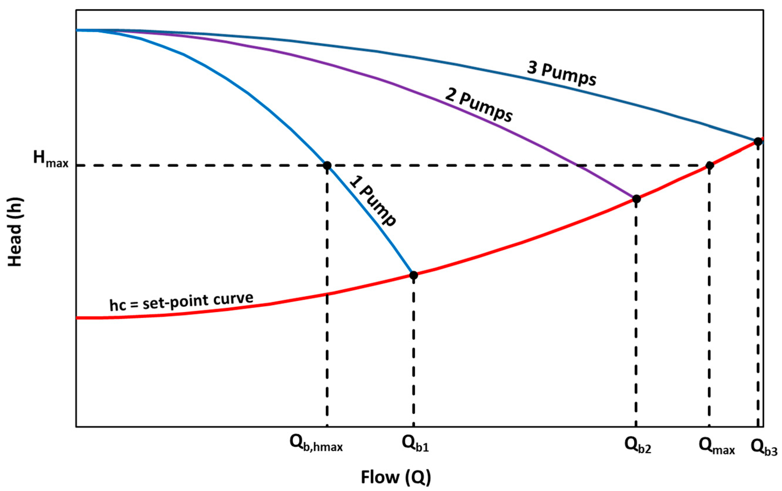
In the pumping control system of the classic method, the total number of pumps that that are calculated determines the number of flow operational ranges. These ranges are defined by the terms (Q_b1, Q_bi, …, Q_bn), where the term Q_bi is the maximum flow that can be supplied when there are i pumps in operation if the control system pretends that the head added by the pump is the same at the required head of the set-point curve. In other words, Q_bi is the intersection between the set-point curve and the head curve of i pumps. In this way, the term i take values from 1 to n, where n is the total number of pumps of the pumping station (Figure 1). The term H_max refers to the total dynamic head when the demand flow is maximum (Q_max).

In the classic method, when demand flow (Q) is in the range (0 < Q < Q_b1), one pump supplies the flow demand at N rotational speed to follow the set-point curve, where N could have values from (0 < N < N₀) and N₀ corresponds to the nominal rotational speed. On the other hand, when the flow (Q) is in the second range (Q_b1 < Q < Q_b2), one pump operates at 100% of nominal speed (N₀) and the second pump operates at a correspondent (N) rotational speed, thus it follows the set-point curve. Another alternative is that the two pumps operate at a same correspondent (N) rotational speed following the set-point curve. When the flow (Q) is in the range (Q_b2 < Q < Q_b3), two pumps work at 100% of nominal speed (N₀) and the third pump works at a (N) rotational speed following the set-point curve. Other alternatives of operation in this last range are one pump works at 100% nominal speed (N₀) and two pumps work at the same correspondent (N) rotational speed following the set-point curve, or three pumps operate at the same correspondent (N) rotational speed that follows the set-point curve.

The idea of this proposed methodology of pumping station design is to determine the optimal number of pumps and the optimal pumping configuration of the control system in every flow rate to minimize the energy. This methodology starts with a set-point curve of the system that determines the conditions of flow and head (Q, H) required at the end of the pump and with a set pump model. Using the operational flow range of the classic method, different pumping configurations are tested, combining FSPs and VSPs and calculating the consumed energy in every configuration to determine the optimal number of FSPs and VSPs in operation. These configurations are determined by adding a pump to the minimum required number of pumps until the minimum consumed energy is obtained. Finally, the results of energy of the different pumping configurations determine the optimal number of FSPs and VSPs in every flow rate.

In summary, the operational flow ranges and the number of required pumps of the control system of the classic method are used only as reference in this proposed methodology. In order for the methodology to be systematized for any pump model, the set-point curve and the characterized curves of the pump model are expressed in a dimensionless form, where these terms are in relation to the best efficient point of the pump.

Before describing the mathematical formulations and the process of this methodology, it is important to highlight several assumptions of this methodology. This methodology is adapted only to closed systems. However, this methodology could also be applied to elevated storage systems if it uses the head and the flow (H, Q) curves that could be supplied a pump as references. In addition, it is assumed that pumping stations are configurated in parallel and are equipped with pumps of the same characteristics. Another assumption is that the type of demand is for urban consumption and does not change through the time. Furthermore, it is assumed that the suction head of the pump is constant and does not change. It is important to mention that the main objective of this proposed control system is to determine the most suitable pumping configuration to obtain the optimal consumed energy. This work does not consider any kind of cost, including investment cost, operational cost, and maintenance cost, in the process of this methodology. In future studies, these costs could be considered for this proposed methodology of pumping station design.

2.2. Mathematical Formulation

The total dynamic head curve of a pump (H) and the efficiency curve of a pump (η) are in function of the flow (Q). When a pump rotates with different rotation speeds, the total dynamic head curve and the efficiency curve are affected by the rotational speed that is defined by the term (α). This term is the relation between the real rotational speed of the pump (N) and the nominal speed (N₀). Taking as reference the affinity laws, both curves are expressed as the following expressions.

$$H=H_1{\alpha }^2-{\alpha }^{\left(2-B\right)}A\times {\left(\frac{Q}{n}\right)}^B$$

(2)

$$\eta =E\times \left(\frac{Q}{\alpha ·n}\right)-F\times {\left(\frac{Q}{\alpha ·n}\right)}^2$$

(3)

$$\alpha =\frac{N}{N_0}$$

(4)

The terms H₁, A, B, E, and F in the previous equations are coefficients that characterize the pump, and the term n is the number of pumps that conforms the pumping system.

The hydraulic power represents the energy of the pump when supplied with some flow with a certain head pressure. It is directly proportional to the specific weight of the water (γ), the flow rate (Q), and the total dynamic head (H). Even though the efficiency of the electrical motor could be between 90% and 95%, it is assumed that the mechanical power on the shaft (P_a) is equal to the electrical power consumed by the motor-pump group (P). This power includes the hydraulic power and the power losses on the transmission of the shaft. Therefore, the efficiency of a pump is defined as the relation between the hydraulic power and the shaft power. The relation between the consumed power of a pump (P), the mechanical torque (M), and the rotational speed of the shaft (ω) are expressed in the following equation:

$$P=\frac{\gamma ·Q·H}{\eta }=M·\omega =P_a$$

(5)

The methodology presented is based on expressing the equations of a pump in a dimensionless way, taking the BEP of the pump as a reference. Therefore, the reduced terms, including total dynamic head (h), flow (q), efficiency (θ), mechanical torque (β), and power (π), are obtained by the relation between the values of these variables and the values of the BEP.

$$h=\frac{H}{H_0} ; q=\frac{Q}{Q_0} ; \theta =\frac{\eta }{{\eta }_0} ; \beta =\frac{M}{M_0} ;\pi =\frac{P}{P_0} ; \alpha =\frac{N}{N_0}$$

(6)

Taking as reference the affinity laws and the previously described terms, the head pressure curve and the efficiency curve in a dimensionless form are expressed as the following equations.

$$h=h_1{\alpha }^2-{\alpha }^{\left(2-B\right)}\times a\times {\left(\frac{q}{n}\right)}^B$$

(7)

$$h_1=\frac{H_1}{H_0} ;a=\frac{A\times Q_0^B}{H_0}$$

(8)

$$\theta =e\times \left(\frac{q}{\alpha \times n}\right)-f\times {\left(\frac{q}{\alpha \times n}\right)}^2$$

(9)

$$e=\frac{E\times Q_o}{{\eta }_0} ;f= \frac{F\times Q_o^2}{{\eta }_0}$$

(10)

$$\pi =\frac{q\times h}{\theta }=\beta \times \alpha$$

(11)

Before analyzing a pumping control system, is important to define the set-point curve. This curve references the demand flow (Q) and the total dynamic head required (H_c) to satisfy the minimum required pressure of the user’s demand at the critical node. The set-point curve is defined as the following expression.

$$H_c=\mathsf{\Delta }H+R\times Q^c$$

(12)

The term ΔH refers to the static head that is defined as the difference of elevations between the axis suction of the pump and the critical node and adding the minimum required pressure of the critical node. The term R is a constant value because the type of demand does not change through time, is associated with the energy losses in the system, and is defined as the resistance of the flow presented in the pipelines. Finally, the term c is an exponent that depends on the characteristic of the system. The terms R and c are obtained by a regression adjustment from the points (H_c, Q) of the set-point curve to the expression (12). Taking as reference the dimensionless terms in a pumping system, the dimensionless form of the set-point curve leads to

$$h_c={\lambda }_1+r\times q^c$$

(13)

where the term λ₁ is defined as the relation between the static head (ΔH) and the nominal head of the pump (H₀), and the term r is associated with energy losses R and the nominal point of the flow and the head of the pump (Q₀, H₀).

$${\lambda }_1=\frac{\mathsf{\Delta }H}{H_0} ; r=\frac{R\times Q_0^c}{H_0}$$

(14)

In order to design a pumping control system, it is important to determine the rotational speed (α) of the pump, thus the pumping system follows the set-point curve. This type of control system we named the flow control system, and it is the focus of this work. However, if the control system aims to maintain a constant head pressure in the pump station (pressure control system), the process is similar. This rotational speed is calculated in an iterative form by setting values of rotational speed on the pumping curve Equation (7) and the set-point curve (13) until the head pressure is the same on both equations.

In order to estimate the efficiency of a pump using a VFD, the affinity laws are used in the equation of the efficiency curve. As it was mentioned previously in the introduction, the affinity laws present an incongruence to calculate the efficiency [39]. However, Coelho and Andrade-Campos [41] proposed an expression that corrects the inaccuracy of the affinity laws. This expression (15) relates the real efficiency or the corrected efficiency (η₂) when the rotational speed of a pump is (N₂) and the estimated efficiency (η₁) when the rotational speed is (N₁). From equation (16), a correction factor f(α) is defined. This factor corrects the efficiency of the pump estimated by the affinity laws

$$\frac{{\eta }_2}{{\eta }_1}=1-{\left(1-\frac{N_2}{N_1}\right)}^3$$

(15)

$$f_{\left(\alpha \right)}=\frac{{\eta }_2}{{\eta }_1}=1-{\left(1-\alpha \right)}^3$$

(16)

On the other hand, the reduced mechanical torque (β) could have values greater than the unit in some cases. In a VSP, a reduced mechanical torque (β_v) is defined by the relation between a VSP’s mechanical torque (M) and the maximum torque of the pump (M_max). Thus, β_v is expressed as:

$${\beta }_v=\frac{M}{M_{máx}}$$

(17)

Additionally, the mechanical torque of the pump β and the torque of the VSP could be related through the following expression:

$${\beta }_v=\frac{\beta \times M_0}{M_{m\mathsf{á}x}}=\frac{\beta }{{\beta }_{max}}$$

(18)

The term β_max is the maximum reduced torque of a pump when the rotational speed is nominal (α = 1) and the flow is (q = q_max). Taking as reference the definition of β, the term of β_max is expressed as:

$$\beta =\frac{q\times h}{\theta \times \alpha }=\frac{(h_1-a\times q^B)\times \alpha }{e\times \alpha -f\times q}$$

(19)

$${\beta }_{max}=\frac{q_{max}\times h}{\theta }=\frac{h_1-a\times q_{max}^B}{e-f\times q_{max}}$$

(20)

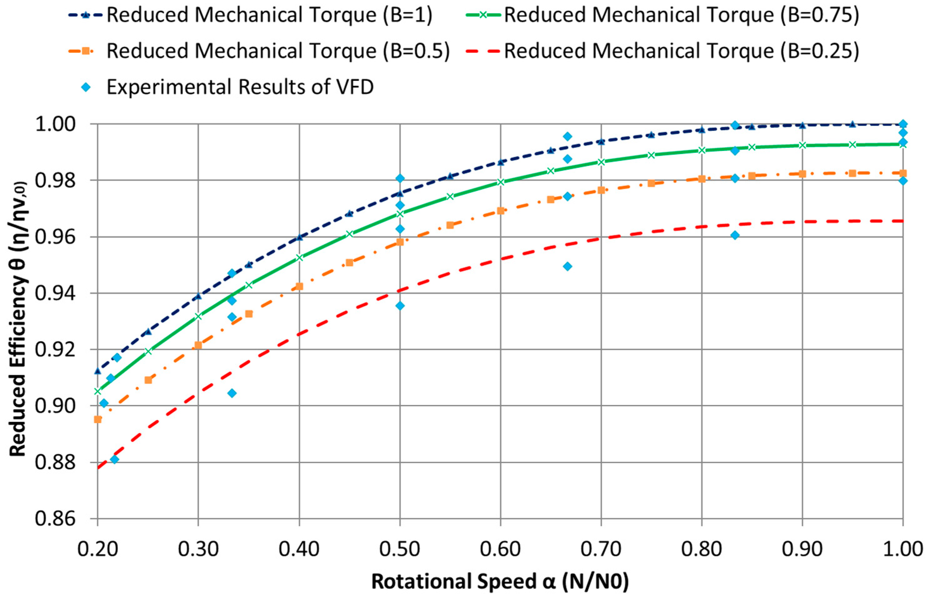
Another important aspect to consider in the energetic analysis of VSPs is the decrease of the efficiency system because of the frequency inverter performance. As it was mentioned in the introduction section, there are several works such as Europump and the Hydraulic Institute (2004) that analyze energy losses in the VFD device relating rotational speed and mechanical torque. They developed experimental essays of different frequency inverters, evaluating the performance with different mechanical torque and different rotational speeds. The aim of this methodology is to develop an expression that best adjusts to the experimental essays of Europump and the Hydraulic Institute [42]. As a result, the expression that best adjusts to the performance essays is:

$${\eta }_v={\eta }_{v,0}\times \left({\beta }_v^{k_1}-k_2\times {\left(1-\alpha \right)}^{k_3}\right)$$

(21)

In this previous equation, η_v is the performance of VFD. This value is determined by the mechanical torque of the VSP (β_v) and the rotational speed (α). The coefficients that best fit the efficiency curve of frequency inverters essays realized by Europump and the Hydraulic Institute [42] are obtained by regression adjustment from experimental tests. These values are k₁ = 0.025, k₂ = 0.16, and k₃ = 2.71. The Figure 2 shows the adjustment of the developed expression by regression technics with the experimental essays of the VFD, where the horizontal axis represents the rotational speed (α) and the vertical axis represents the reduced efficiency of the VFD (θ_v). The different type of lines represents the adjustment curve of the efficiency of VFD for different reduced mechanical torque (β) and the points represent the experimental essays obtained from Europump and the Hydraulic Institute [42].

The performance of the frequency inverter in a reduced form is expressed as the following expression:

$${\theta }_v=\frac{{\eta }_v}{{\eta }_{v,o}}={\beta }_v^{k_1}-k_2\times {\left(1-\alpha \right)}^{k_3}$$

(22)

Finally, the global efficiency of the pumping system (η_c) and its reduced form (θ_c) should be defined considering the correction of the inaccuracy of the estimated efficiency and the performance of the frequency inverter. Mathematically, they can be expressed as:

$${\eta }_c=\eta \times f_{\left(\alpha \right)}\times {\eta }_v$$

(23)

$${\theta }_c=\theta \times f_{\left(\alpha \right)}\times {\theta }_v\times {\eta }_{v,o}$$

(24)

The total consumed energy of a pumping system is expressed as the following equation:

$${\pi }_T=\frac{q\times h}{{\theta }_c}=\beta \times \alpha$$

(25)

This last expression allows evaluating the consumed energy in dimensionless form for the different alternatives of pumping configuration for every flow range. Finally, this analysis determines the optimal number of FSPs and VSPs in operation that is the objective of the methodology.

2.3. Process of the Optimization Methodology

As it was previously explained in the mathematical formulations, the terms of the characteristic curves of the pump and the set-point curve are expressed in dimensionless forms that are in relation to the BEP of the pump. In this way, the flow of the optimization analysis of the pumping system is expressed in a reduced form (q) that is the relation between the supplied flow and the nominal flow of the pump (Q/Q₀). In the same way, the total consumed energy is expressed in a reduced form (${\pi }_T$) that is the relation between the consumed power of the pump and the nominal power of the pumps ($P/P_0$). In order to explain how the total operational range (q_min < q < q_max) is expressed in this methodology, the following

Table 1. Examples of flow representation of the system with the proposed method.

Pump Model Q0 (L/s)	(Qmin)	(Qmax)	qmin	qmax
100	20	200	0.2	2
50	20	200	0.4	4
40	20	200	0.5	5
20	20	200	1	10

shows some examples of the limits of the operational range that are minimum demand flow (Q_min) and maximum demand flow (Q_max) and its equivalency in reduced terms (q_min and q_max) with different pump models.

This optimization process starts with a set pump model of the pumping station and the requirements of (Q, H) of the system (the set-point curve) and a set flow range (q_max < q < q_max). It is important to remind the reader that this process is focused with the control system that allows the pumping station to follow the set-point curve (flow control system). With these data, the minimum required number of pumps of the pumping station according to the classical method established is determined. It is obtained by the relation between the flow of the system and the flow that one pump supply with the maximum total dynamic head requires (Q_max/Q_b,hmax).

Once the total number of pumps is obtained, the flow operational range of the pumping system is determined. It is important to remind the reader that the total number of pumps (N_pumps) determines the same number of operational ranges in the classic method. In this way, every operational range is set by the term i, where this term varies from 1 to N_pumps, and every term of i determines the number of pumps in operation in every flow operational range. For example, if the number of pumps is three pumps, there are three operational ranges. In the first, the second, and the third operational range, there are one pump, two pumps, and three pumps in operation, respectively. In summary, this proposed methodology takes as reference the operational range of the classical method to analyze the optimal number of pumps and pumping configuration in every flow rate.

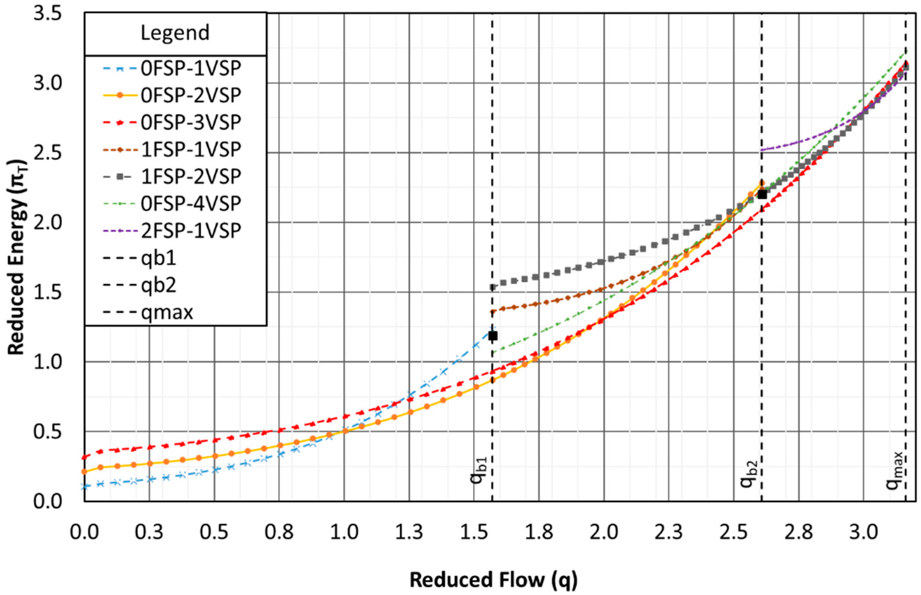
The next step is to set the number of pumps in study to the minimum required number of pumps. At this point, all the possible pumping configurations in operation with FSPs and VSPs are determined. For example, in the first range of operation, the only possibility of operation is 1 VSP. Conversely, it is not possible evaluate 1 FSP, because it exceeds the requirements of the systems and cannot follow the set-point curve. In the second range, the possibilities are 2 VSPs or 1 FSP with 1 VSP, whereas, in the third range, the possibilities are 3 VSPs or 1 FSP with 2 VSPs or 2 FSP with 1 VSP. Then, the energy for every pumping combination in every flow rate is evaluated and the minimum consumed energy is determined.

Once the consumed energy with the number of pumps in study is analyzed, the current number of pumps in study is incremented in a unit pump. With this incremental number of pumps, all the pumping combinations are determined once again and the consumed energy in every flow rate is evaluated. Then, the minimum consumed energy is determined.

If the minimum consumed energy with the current number of pumps is not incremented with respect to the last number of pumps, the current number of pumps is increased once more and the process is repeated. Nevertheless, if the minimum consumed energy of this increment of pumps is incremented with respect to the last number of pumps, the process is stopped, and the optimal number of pumps is the last number of pumps in study.

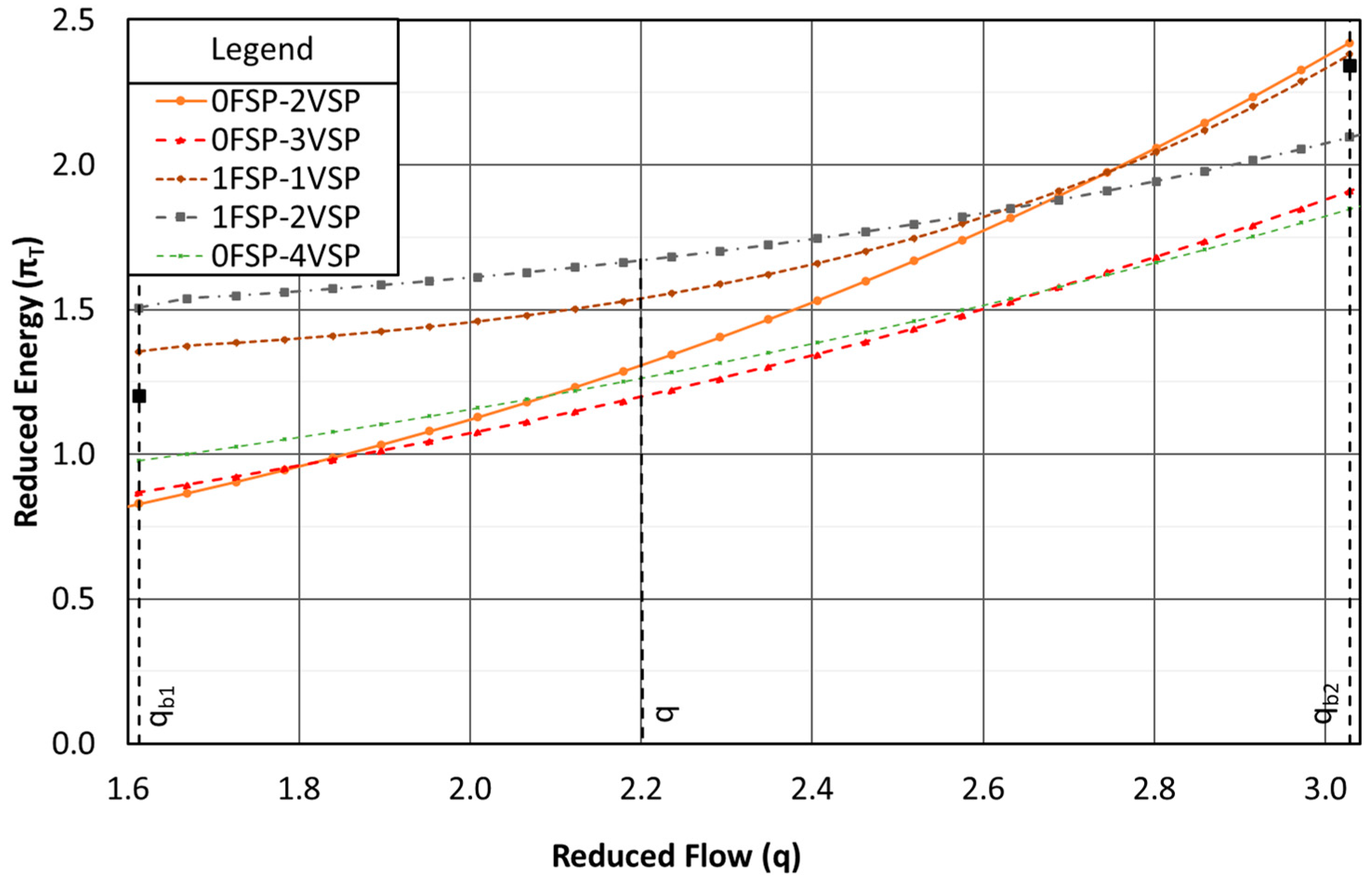
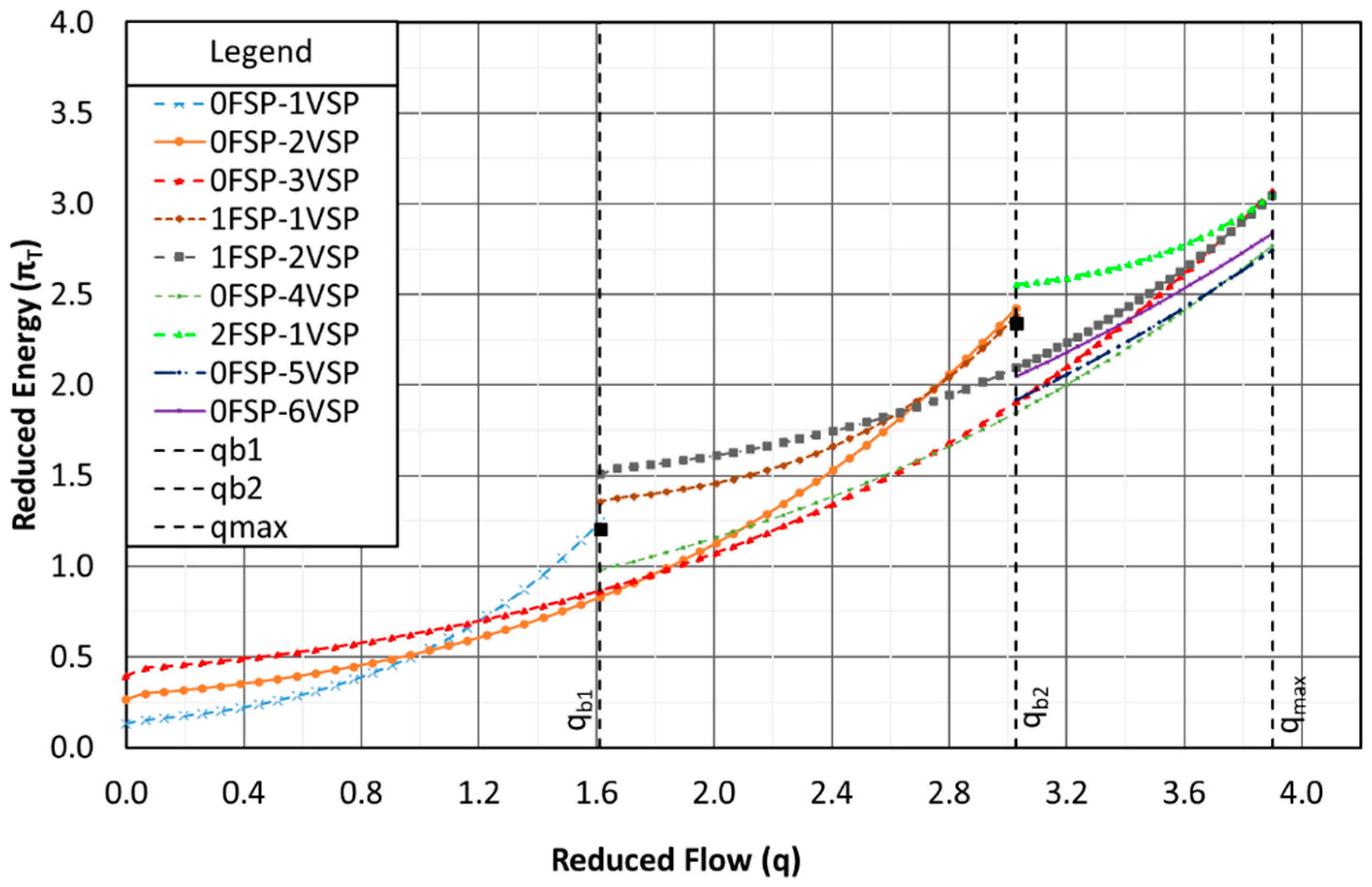
Figure 3 shows an example with a set flow of how the consumed energy evolves as different pumping combinations are evaluated. As an example, it is assumed that the calculated number of pumps for a set pump model is three pumps, thus there are three operational ranges. Figure 3 shows different pumping combinations for the second range (q_b1 < q < q_b2). For example, a reduced flow (q = 2) is in the second range, the minimum required pumps is 2 pumps, and the possible combinations are 2 VSPs or 1 FSP with 1 VSP. Then, 3 and 4 pumps are added in this flow, and the possible combinations that are evaluated are 0 FSP-2 VSPs, 1 FSP-1 VSP, 0 FSP-3 VSPs, 1 FSP-2 VSPs, and 0 FSP-4 VSPs. There are more pumping combinations for 4 pumps, such as 1 FSP-3 VSPs. However, it is not necessary to evaluate this combination because the combination 1 FSP-2 VSPs is not optimal, and it is inferred that the combination 1 FSP-2 VSPs consumes more energy. In summary, it is observed in Figure 3 that the optimal pumping combination in energy terms for a flow (q = 2) is 0 FSP-3 VSPs.

3. Case Studies

This paper considers two study cases to apply the methodology. The first case is the TF network and the second case is the E1 network. In order to design the pump station, it is necessary to set a model pump that supplies the requirements of the network. The objective of this work is to determine the most suitable control system in energy terms, but this work does not approach the selection of the pump model. Therefore, TF network and E1 network are not focused on the pump model selection. These case studies are only focused on analyzing the optimal control system that could be obtained from a certain model pump. In this way, the pump models are set in both case studies, and then the optimal operational mode is determined.

3.1. TF Network

The information of the TF network is obtained from Leon Celi’s work [44]. This network is composed of four pumping stations (PSs), and these PSs are directly pumped to the consumers. The suction of the pump and the axis of the pump have the same level. Hence, the suction head is zero.This study only obtains the values of the set-point curve and the flow rates supplied from every supply source. In order to explain the process of the proposed method, the pumping station (PS4) of the TF network is used as an example. For the other pumping stations of the TF network, the process is the same as that explained in PS4 (Supplementary Materials). The flow rates obtained in PS4 vary from 6.80 L/s (Q_min) to 33.50 L/s (Q_max), and the average demand flow (Q_m) is 17.2 L/s. Since several possible solutions of pump models for the pump station exist, a pump model is applied in the methodology. The characteristics of the model pump and the set-point curve in dimensional and dimensionless forms are described in

Table 2. Characteristic terms of the pumping curve.

Pumping Curve
Characteristic Terms		Reduced Terms
H1 (m)	102.75	h1	1.33
A$\frac{\mathrm{m}}{{(\mathrm{L}/\mathrm{s})}^2}$	0.2290	a	0.33
B	2	B	2
E	0.1228	e	1
F	5.80 × 10−3	f	2
Qo (L/s)	10.59	qo	1
Ho (m)	77.06	ho	1
Qbmax (L/s)	21.18	qbmax	2
ηo (%)	65	θ	1
Qmax (L/s)	33.50	qmax	3.16
Qb,hmax (L/s)	11.27	qh,max	1.06

and

Table 3. Characteristic terms of the set-point curve.

Set-Point Curve
Characteristic Terms		Reduced Terms
ΔH (m)	28.18	λ	0.3657
R$\frac{\mathrm{m}}{{(\mathrm{L}/\mathrm{s})}^2}$	4.05 × 10−2	r	0.0589
c	2	c	2
Hmax (m)	73.63	hmax	0.95

.

The minimum number of pumps required for this model pump in a classic system is three pumps. The operational ranges in a classic system are: 0 < q < q_b1, q_b1 < q < q_b2 and q_b2 < q < q_max. These ranges of the classic system are used as reference to develop the proposed methodology.

3.2. E1 Network

The E1 network is conformed with one pumping station and three consumption nodes. This network is composed of four pumping stations, and these PSs are directly pumped to the consumers. The suction of the pump and the axis of the pump have the same level. Hence, the suction head is zero. The average demand flow is Q_m = 246 L/s, and the maximum demand flow is Q_max = 312 L/s. This network is chosen with two different objectives. The first one is to demonstrate that the application of the proposed methodology is valid regardless of the network considered. Furthermore, this is a methodology focused solely on the requirements of the pumping station. The second objective is to show how the selection of the pump model for a certain pumping station is associated with the definition of a different control system in each case. For this reason, in this network, three different models of pumps are analyzed and compared. These models are selected so that the required number of pumps in the classic system is three pumps. The parameters of the characteristic curves of these three pump models are described in

Table 4. Characteristic values of each pump model.

Pump Model	A	B	C
H1 (m)	61.67	49.33	42.67
A$\frac{\mathrm{m}}{{(\mathrm{L}/\mathrm{s})}^2}$	0.0024	0.001	0.0008
B	2	2	2
E	2.05 × 10−2	1.24 × 10−2	1.32 × 10−2
F	1.28 × 10−4	5.50 × 10−5	5.70 × 10−5
Q0 (L/s)	80	112.5	115
H0 (m)	47	37	32
Qbmax (L/s)	160	225	230
H0 (%)	82	70	76
Qmax (L/s)	312	312	312
Qb,hmax (L/s)	113.39	136.43	119.26

. The behavior of the E1 network from the pumping station point of view is defined by its set-point curve. The parameters of the set-point curve for this case are shown in

Table 5. Set-point curve of the pumping station of the E1 network.

Parameter	Value
ΔH (m)	20.00
R (m/(/s)2)	1.15 × 10−4

.

4. Results and Discussions

4.1. TF Network

4.1.1. Results

The different alternatives of pumping configurations that are evaluated in reduced energy terms are the result of adding a pump to the minimum required number of pumps in every operational range of the classic system until obtaining the optimal pumping configurations in energy terms. When the consumed energy of the current pumping configuration increases with respect to the last pumping configuration, it is not necessary to evaluate another configuration by adding a pump because it is implicit that the consumed energy of this configuration will be greater than the other configurations. Therefore, there are seven different pumping configurations evaluated that include: 1. zero FSP with one VSP (0 FSP-1 VSP); 2. zero FSP with two VSPs (0 FSP-2 VSP); 3. zero FSP with three VSPs (0 FSP-3 VSP); 4. one FSP with one VSP (1 FSP-1 VSP); 5. one FSP with two VSPs (1 FSP-2 VSPs); 6. zero FSP with four VSPs (0 FSP-4 VSPs); and 7. two FSPs with one VSP (2 FSPs-1 VSP). These configurations evaluated in energy terms are represented in Figure 4.

The broken vertical lines in Figure 4 represent the limit flows of the operational ranges in the classy system. These limit flows in reduced terms are: 1.57 L/s (q_b1), 2.61 L/s (q_b2), and 3.16 L/s (q_max). The horizontal axis of Figure 4 represents the reduced flow rate (q) of the pump station, whose values are from (0 < q < q_max). The vertical axis represents the reduced consumption power (π_T) of pumping configurations. These terms (q and π_T) are related to the BEP of the pump (Q₀ and P₀). The notation of the legends is defined as (n FSPs-m VSPs), where the terms n and m are the number of FSPs and VSPs, respectively. Every legend illustrates the reduced power curve of the different pumping configurations.

There are some important points to highlight in the generated energy graph. There are jumps of energy when the pumping configuration changes from zero FSP with one VSP (0 FSP-1 VSP) to one FSP with one and two VSPs in operation (1 FSP-1 and 2 VSPs). Another energy jump is produced when the configuration changes from zero FSPs with two VSPs (0 FSP-2 VSPs) to two FSPs with one VSP (2 FSPs-1 VSP). These jumps are produced because, when a pump starts to work (q = 0), the consumed energy of a pump is not zero, and the mechanical torque consumes energy even though the efficiency of the pump is zero.

In the first range of the classic system (0 < q < q_b1), the configuration with zero FSPs with one VSP (0 FSP-1 VSPs) starts to be the optimal configuration until the range 0 < q < 1.01. After this range, the optimal configuration is zero FSPs with two VSPs (0 FSP-2 VSPs) until the end of the first range (1.01 < q < q_b1). In the second classic range (q_b1 < q < q_b2), the configuration 0 FSP-2 VSPs continues to be optimal until the range q_b1 < q < 1.99. Then, the optimal configuration is 0 FSP-3 VSPs until the end of the second range (1.99 < q < q_b2). Finally, at the beginning of the third classic range q_b2 < q < q_max, the configuration 0 FSP-3 VSPs continues to be the optimal configuration until the range q_b2 < q < 2.92. At this point, the optimal configuration changes to 1 FSP-2 VSPs until the reduced flow reaches the value of 3.03. Finally, if this reduced flow continues growing, the optimal configuration changes to 2 FSPs-1 VSP until the maximum demand flow (3.03 < q < q_max).

It is important to mention that it is not necessary to continue increasing the number of pumps. For example, when the flow is q_max, the configuration 0 FSP-4 VSP is not optimal. If the number of pumps continues to increase to five pumps, all the combinations of five pumps increase the consumed energy. In fact, it is not necessary to evaluate other combinations of four pumps, such as 1 FSP-3 VSP, 2 FSP-2 VSP, or 3 FSP-1 VSP, because it is inferred that the consumed energy of these combinations will be greater than the optimal configuration in this q_max that is 1 FSP-2 VSPs.

4.1.2. Discussion

Table 6. Resume of the optimal pumping configuration. FSP: fixed speed pumps; VSP: variable speed pumps.

	Optimal Pumping Configuration
Flow Range	No. FSP	No. VSP	No. Pumps
0 < q < 1.01	0	1	1
1.01 < q < 1.99	0	2	2
1.99 < q < 2.92	0	3	3
2.92 < q < 3.03	1	2	3
3.03 < q < 3.16	2	1	3

shows a resume of the optimal number of FSPs and VSPs in operation for every flow range, and Figure 5 represents the number of operating pumps (N_pumps) in relation to the demand flow rate (q). As it can be seen in this figure, the shape of the graphic of N_pumps has several steps. Every step represents the limit range of the number of pumps in operation, and the vertical lines in the figure represent the flow limits of the operational ranges in the classic system. Even though Figure 5 shows three steps, the proposed system has five different operational ranges or pumping configuration because, in the range of three pumps, there are changes on pumping configuration. For example, in this range, the configuration changes from 0 FSP-3 VSPs to 1 FSP-2 VSPs and finally to 2 FSPs-1 VSP.

In Figure 4, one can see when the demand flow (q) is close to the limit operational flow (q_max), the configurations that combine FSPs and VSPs tend to get better results in energy terms than configurations using only VSP. Therefore, the performance of the frequency inverter affects a significant form of the global efficiency of VSPs, thus these pumps consume more energy than FSPs.

Therefore, both systems (classic and proposed) have different operational ranges but have the same total number of pumps required for the design of the pumping station. Besides, the limits of the flow ranges are not the same in both systems. For example, the changes in number of pumps in operation from one to two pumps and from two to three pumps take place before than the classic system. Therefore, the operational mode of this proposed system is different than the classic system and leads to energy savings.

In summary, in the first case study (TF network), the total number of pumps is three pumps, which is the same as the classic system. However, there are more changes of pumping configurations than the classic method. In fact, there are five different optimal pumping configurations throughout the range study (0 < q < q_max), while the classic method has three different pumping configurations in the range study.

4.2. E1 Network

4.2.1. Results

The methodology proposed in this work performs the energy analysis using reduced variables. For this reason,

Table 7. Reduced values of the different pump models.

Pump Model	A	B	C
qmax	3.90	2.77	2.71
qb,hmax	1.42	1.21	1.04

and

Table 8. Reduced values of the set-point curve for each pump model.

Pump Model	A	B	C
λ	0.42	0.54	0.62
r	0.015	0.039	0.047
hcmax	0.66	0.84	0.97

show the dimensionless values of both the characteristic parameters of the pumps and the characteristic values of the set-point curve. It should be noted that the three pump models have the same dimensionless shape of their head and efficiency curves. Therefore, their values in reduced variables are the same. The reduced values of the characteristic curves of the pumps are: h₁ = 1.33, a = 0.33, b = 2, e = 1, f = 2, and q_b.max = 2. Obviously, there are values that are different depending on the pump model. The maximum flow to supply is fixed. However, the value of the maximum reduced flow (q_max) will be different in each model since the reduced variables are defined based on the BEP. Likewise, the reduced flow supplied by each pump model will also be different when the head is equal to the maximum required by the setpoint curve (q_b,hmax).

In order to present the application of the methodology, Figure 6 shows an example of the results in the case of using Model A. The horizontal axis is represented by the dimensionless flow (q) of the total rage (0 < q < q_max), whereas the vertical axis represents the dimensionless total consumption power (π_T) of the pumping configurations. These terms (q and π_T) are related to the BEP of the pump (Q₀ and P₀). The evaluation of the consumed energy for each pumping flow can be observed with different control configurations. These different control settings are determined by the number of FSPs and VSPs. In the case of FSPs, the pumps that are running rotate at their nominal speed, while the VSPs adjust their rotation speed in such a way that the operating point is adjusted to the setpoint curve. As it can be seen in Figure 6, there are nine different curves of reduced energy of the different pumping configurations evaluated for the pump model A. There are three limit operational flows in the classic system represented by vertical broken lines in Figure 6. These flow limits are: q_b1 = 1.61, q_b2 = 3.02, and q_max = 3.16.

4.2.2. Discussion

The optimal numbers of FSPs and VSPs obtained in every flow rate for the three different pump models analyzed are defined by

Table 9. Optimal number of FSD and VSD pumps for different pump models.

Model A			Model B			Model C
Flow Range	No. of FSP	No. of VSP	Flow Range	No. of FSP	No. of VSP	Flow Range	No. of FSP	No. of VSP
0 < q < 1.03	0	1	0 < q < 1.17	0	1	0 < q < 1.25	0	1
1.03 < q < 1.84	0	2	1.17 < q < 2.15	0	2	1.25 < q < 2.10	0	2
1.84 < q < 2.75	0	3	2.15 < q < qmax	0	3	2.10 < q < 2.33	1	1
2.75 < q < 3.76	0	4				2.33 < q < 2.59	0	3
3.76 < q < qmax	0	5				2.59 < q < qmax	1	2

. This table illustrates the results obtained with each model with different configuration control systems.

The proposed configuration system mode for the second and the third pump models is similar to the classic system because the total optimal number of pumps is three pumps, as it is established in the classic system, whereas, in the first pump model, the optimal number of pumps is five pumps, which is more than the minimum required of the classic system. Another important point to highlight is the optimal head (H₀) of the first model pump that is further away from the maximum head of the set-point curve (H_cmax) than the optimal head (H₀) of the second and the third models, where H₀ is close to H_cmax. The optimal number of pumps in every flow range of the three different model pumps can be visualized in Figure 7. Because the three model pumps have different BEPs and the reduced flow rate is in relation to the nominal flow (Q₀), the maximum operating limits (q_max) of the three model pumps have different values.

Even though the total number of pumps of the optimal configuration of the pump A model has more pumps than models B and C, the optimal configuration of model A consumes less energy in all flow rates than the other pump models; this is corroborated in Figure 8. This figure compares the consumed energy of the optimal pumping configurations of the three model pumps analyzed. It is important to mention that the consumed energy (P_T) and the flow rate (Q) have to be represented in dimensional forms to compare the consumed energy of the optimal configuration of the three model pumps in a better way. The flow rates in dimensional form (Q) are the same for the three model pumps, but the flow rates in a dimensionless form (q) are different for the three pumps because the variable (q) is in function of the BEP and the three pumps have different BEPs.

In summary, the E1 network was analyzed using both systems and three different pumps. One model pump of the three studied indicated that the total number of pumps in the proposed system was greater than the classic system and also obtained an energy saving in comparison with the classic system.

5. Conclusions

Much of the scientific research on pump scheduling takes, as a starting point, a number of pumps previously set according to the classic system operation. This assumption could lead to not achieving the optimal result in terms of energy consumed in the PS because it has not been optimally designed. Another limitation presented by some studies on the operation of pumping stations is they do not consider the effect of the performance of the frequency inverters on the global efficiency of a pumping station when a VSP changes its rotational speed. In the best case, a constant efficiency of frequency inverter on the global efficiency is assumed. This may generate inaccuracy to determine the consumed energy of this pump, and it affects the PS global energy consumed. Therefore, the purpose of this present work is to discuss the classic system operation, determining the optimal number of pumps for every flow rate so that the consumed energy be optimal. Another contribution of this work is to consider that the efficiency of the frequency inverters of the VSPs varies depending on the load. In this way, the determination of the global energy optimum takes into consideration the efficiency of these devices.

The discussion about the classic operating system of a pumping station is relevant since different operating rules lead to lower energy consumption. Besides, it is important to analyze the optimal number of pumps for every flow rate because it determines the total number of pumps in an optimal pumping station design.

This study accomplishes the development of a methodology that analyzes how the pumping curve and the set-point curve influence the determination of the optimal number of FSPs and VSPs for each flow rate. The main idea of this methodology is to express the set-point curve and the pumping curve in a dimensionless form in relation to the BEP of the pump so that the methodology is more systematized to analyze different case studies. In this way, several pumping configurations are added and evaluated in energy terms to obtain the configuration with the minimum consumed energy.

The results obtained in both study cases allow us to conclude that the performance of a frequency inverter has a great influence on the global efficiency of a VSP, especially when the demand flow is close to the limits of the classic operational ranges (q_b2, q_b3, q_max). In fact, there could be cases where the consumed energy on VSP is higher than FSP. Therefore, a combination of FSPs and VSPs consumes lower energy than a configuration only with VSP.

The number of FSPs and VSPs in operation cannot be inferred in a simple form as is commonly done in the classic system. It requires a deep analysis on the control system, where the optimal number of pumps depends on several factors such as the BEP of the pump, the energy losses on the set-point curve, and how far or close the optimal head of the pump is to the maximum head of the set-point curve. For example, the optimal configuration of the pump of the TF network and the second and the third models pumps of the E1 network indicated that the total optimal number of pumps is the same as the minimum required pumps in the classic system. However, the optimal number of pumps in the first model pump of the E1 network is more than the minimum required in the classic system.

Furthermore, the minimum required pumps of a pumping system is not necessarily the best option in energy terms. In fact, the first pump model of the E1 network has an optimal number of pumps greater than the second and the third pump models, and at the same time, this first pump model is the best option in energy use. In summary, the total number of pumps associated with a pump model in a pumping station is not necessarily a decisive factor to determine the best alternative in energy terms, but it requires a deep analysis in the control pumping system configuration.

One limitation of this proposed methodology is that the set-point curve expression is adapted to closed networks. However, the general procedure of this methodology is similar to networks with a storage system. Another limitation is that the pumping curve, the pump efficiency curve, and the set-point curve are adjusted in exponential expressions. Despite this, this methodology is valid to be applied in any case study of pumping station designs. Furthermore, the expression of frequency inverter efficiency is adjusted according to experimental works that were previously mentioned in the methodology section. However, this expression is still valid to be considered on the analysis of pumping station operation.

Future research will be to develop a methodology to select the most suitable pump model for a pumping station design including this newly proposed control system operation. Besides, it will consider investment cost, operational cost, and maintenance cost in order to appropriately design a pumping station.