
Invertebrate and Microbial Response to Hyporheic Restoration of an Urban Stream
by
 , , and
Sarah A. Morley
1,* ,
,
Linda D. Rhodes
1,
Anne E. Baxter
2,†,
Giles W. Goetz
3,
Abigail H. Wells
2 and
Katherine D. Lynch
4 1
Northwest Fisheries Science Center, National Marine Fisheries Service, National Oceanic and Atmospheric Administration, 2725 Montlake Boulevard E, Seattle, WA 98112, USA
2
Lynker Technologies, Under Contract to Northwest Fisheries Science Center, Seattle, WA 98112, USA
3
School of Aquatic and Fishery Sciences, University of Washington, 1122 NE Boat St., Seattle, WA 98195, USA
4
Seattle Public Utilities, 700 5th Ave, Suite 4900, Seattle, WA 98124, USA
*
Author to whom correspondence should be addressed.
†
Current affiliation: Watershed Resources Unit, Washington State Department of Ecology, 300 Desmond Drive SE, Lacey, WA 98503, USA.
Water 2021, 13(4), 481; https://doi.org/10.3390/w13040481
Submission received: 1 January 2021
/
Revised: 5 February 2021
/
Accepted: 7 February 2021
/
Published: 12 February 2021
(This article belongs to the Special Issue Cross-Sector Green Infrastructure for Improving Urban Storm Water Quality)
Abstract
:All cities face complex challenges managing urban stormwater while also protecting urban water bodies. Green stormwater infrastructure and process-based restoration offer alternative strategies that prioritize watershed connectivity. We report on a new urban floodplain restoration technique being tested in the City of Seattle, USA: an engineered hyporheic zone. The hyporheic zone has long been an overlooked component in floodplain restoration. Yet this subsurface area offers enormous potential for stormwater amelioration and is a critical component of healthy streams. From 2014 to 2017, we measured hyporheic temperature, nutrients, and microbial and invertebrate communities at three paired stream reaches with and without hyporheic restoration. At two of the three pairs, water temperature was significantly lower at the restored reach, while dissolved organic carbon and microbial metabolism were higher. Hyporheic invertebrate density and taxa richness were significantly higher across all three restored reaches. These are some of the first quantified responses of hyporheic biological communities to restoration. Our results complement earlier reports of enhanced hydrologic and chemical functioning of the engineered hyporheic zone. Together, this research demonstrates that incorporation of hyporheic design elements in floodplain restoration can enhance temperature moderation, habitat diversity, contaminant filtration, and the biological health of urban streams.
1. Introduction
Urban stormwater damages aquatic habitats and the life that they support [1,2]. As native soils and vegetation are replaced by impervious surfaces, tributaries placed into pipes, and floodplains filled in, natural water storage capacity disappears from the built environment [3,4]. Stormwater that runs off this urban landscape short circuits the natural hydrologic regime and delivers toxic contaminants to streams and other receiving bodies [5,6]. The result is poor water quality, lack of physical habitat complexity, and loss of native species—a condition coined the “urban stream syndrome” [7].
The rise of green stormwater infrastructure (GSI) in cities worldwide is an opportunity to improve outcomes for urban streams [8,9]. GSI can take many forms, but the underlying principle is the same: utilize natural processes to capture, filter, and reduce stormwater runoff on site [10,11]. In the natural drainage network, these processes happen in floodplains. These seasonally inundated transitional habitats facilitate exchange of water, sediment, wood, nutrients, and organisms among many other critical ecosystem services [12,13]. Reconnecting urban streams to their floodplains can increase stormwater storage capacity while also restoring ecosystem function [14,15,16].
Floodplain reconnection is thus both a GSI technique and a form of process-based stream restoration [17,18]. Both approaches focus on similar themes of watershed connectivity, and on supporting the natural processes that create and sustain healthy streams and rivers. This connectivity can occur in multiple directions [12,19]: longitudinally from the headwater to the mouth, laterally as the channel migrates within its floodplain, and vertically as surface and groundwater mix in the layer of saturated sediment beneath and adjacent to the stream channel known as the hyporheic zone (HZ) [20].
This subsurface ecotone is critical in flood dampening and groundwater recharge, water temperature regulation, and biogeochemical cycling of nutrients, organic matter, and contaminants [21,22,23,24]. The HZ is also thought to serve as refugia for microorganisms, invertebrates and larval fish during extreme flows and other disturbance events [25,26] While the importance of the HZ to stream ecosystem function has been recognized for some time [21,27,28], scientists have more recently called for the inclusion of hyporheic processes in restoration planning [29,30,31,32,33].
In 2014, the City of Seattle (Washington State, USA) constructed two floodplain reconnection projects with a novel component: an engineered HZ [34]. These pilot projects were undertaken both to reduce flooding and to improve conditions for imperiled salmon populations (Oncorhynchus spp.). The aim was to restore physical processes that sustain stream function by maximizing onsite water, sediment, and wood storage with expanded floodplain and hyporheic capacity; slow erosive peak flows; modulate stream temperature; filter stormwater contaminants; increase instream hydraulic diversity; and ultimately improve stream biological condition.
The hyporheic component of these reconnection projects was guided by a streambed engineering approach designed to increase vertical connectivity, hyporheic residence time and exchange by restoring channel complexity and sediment permeability [34]. Channel width and sinuosity were increased by connecting to an over-excavated inset floodplain; bank armoring and other artificial channel fill were replaced with a deep and wide alluvial gravel corridor; and plunge pools, large wood and impermeable liners were strategically placed to promote hyporheic flow paths. Further background on project design can be found in Bakke et al. [35].
While evidence is building that GSI approaches can locally decrease the quantity and improve the quality of stormwater runoff, benefits to urban streams remain largely untested [1,9]. In order to test performance of these pilot projects, the City of Seattle engaged science partners to evaluate hydrologic [35] and chemical [36] response. We now add to this body of research by reporting on biological outcomes. Thus far, the small body of literature on hyporheic restoration has largely focused on physiochemical effects, such as flow dynamics and chemical transformations [32,37,38]. We are not aware of any research on the response of hyporheic biota to restoration.
Biological processes within the HZ such as organic matter decomposition, nutrient cycling, and contaminant detoxification are largely carried out by invertebrates and microbes [21,22,39,40]. These processes in turn affect availability of particulate and dissolved organic carbon, concentrations of nutrients and contaminants, algal production, and prey availability for fish [41,42,43]. Thus, our monitoring focused primarily on densities and composition of hyporheic invertebrates and microbes, heterotrophic production, and collection of complementary nutrient datasets.
We hypothesized that following restoration, an expansion in the total volume, complexity, and connectivity of hyporheic habitat would result in (1) water temperature modulation, increased (2) hyporheic dissolved oxygen concentration, (3) particulate organic matter and dissolved organic carbon concentrations, (4) heterotrophic production, (5) shifts in microbial taxonomic composition, and (6) increased hyporheic invertebrate density and richness.
2. Materials and Methods
2.1. Study Region
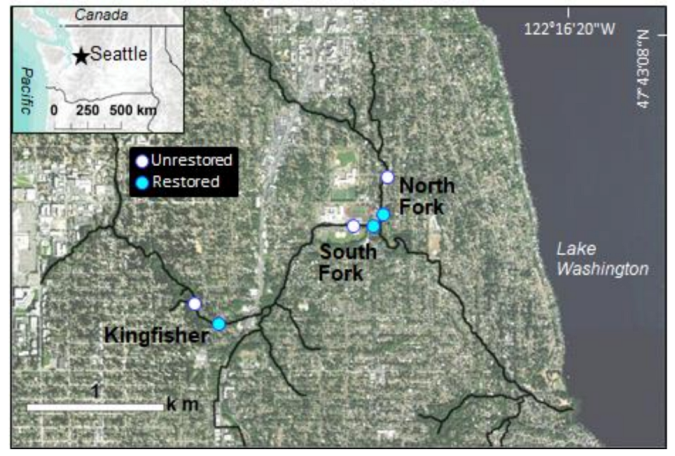
This study took place in the 28.8 km2 Thornton Creek watershed, located between the borders of Seattle and Shoreline in Washington State, USA (Figure 1). Thornton Creek flows approximately 24 km in a southeasterly direction through three major sections—the North Branch (hereafter referred to as North Fork), the South Branch (hereafter referred to as South Fork), and the mainstem—before emptying into north Lake Washington at Matthews Beach. Elevation ranges from 2.5 m at the mouth to 250 m in the headwaters. Mean annual precipitation is 89 cm, received primarily as rain between October and May.
The Thornton Creek watershed is the largest and most urbanized watershed within the City of Seattle. Single-family residences comprise 49% of development within the watershed, with the remaining land use primarily in roads and commercial developments [44]. Over half (61%) of the watershed is covered by impervious surfaces, and the loss of native forest cover across the watershed has severely altered the quantity, timing, and quality of stormwater [45]. This highly modified flow regime further degrades instream physical habitat and water quality [46]. A functioning HZ is largely absent from the majority of Thornton Creek, where only a thin layer of gravel and sand remain atop the compacted streambed [35,47].
The biological health of Thornton Creek is poor. The rate of coho salmon (O. kisutch) pre-spawn mortality is among the highest for the region—an average 80% of adult salmon entering Thornton Creek die with near-total retention of eggs or milt [48]. Resident fish populations lack adequate refuge and spawning habitat [44]. Scores for the Benthic Index of Biological Integrity (B-IBI), a multimetric index based on benthic invertebrates, consistently rate the biological health of Thornton Creek as “poor” to “very poor” [49,50].
2.2. Experimental Design
Our study design compares restored and unrestored stream reaches over multiple years. The focus is two restoration projects on Thornton Creek constructed with an engineered HZ: Kingfisher and Confluence (Figure 1). Kingfisher is located on the south fork of the creek, covers approximately 0.6 hectares, and drains 6.6 km2. The Confluence project is approximately one hectare in size, drains an area of 9.8 km2, and encompasses the north fork, south fork, and mainstem of Thornton creek. We treat Confluence as two separate sites: North Fork and South Fork. For monitoring purposes, we paired each of these three restored reaches (50–75 m in length) with an unrestored reach located between 50 and 350 m upstream (Figure 1).
We began collecting data at all reaches immediately following project completion, which occurred in November of 2014. To maintain seasonal consistency, we sampled yearly thereafter every November until 2017. On each sample event, we collected one surface water and five hyporheic samples from piezometer arrays installed at each reach. Piezometers were constructed of stainless steel, 4 cm in diameter, and had 1.25 cm perforations. We installed piezometers evenly across the length of each reach near pool tail-outs, and buried perforations 15–25 cm below the stream bed to sample the upper layer of the HZ. Piezometers were sealed with bentonite to minimize surface water intrusion.
We used a standpipe and a manual diaphragm pump to extract eight liters of interstitial water for analyses on each sample event. To avoid drawing water down from the surface, extraction speed was dictated by piezometer recharge rate and ranged from 0.25 to 2.50 min L−1. Two-liter surface water samples were also collected from a well-mixed area at the mid-point of each reach. All hyporheic and surface samples were processed independently (i.e., no pooling) and analyzed as described below.
2.3. Sample Parameters
2.3.1. Environmental Covariates
We recorded in situ water quality measurements during each sample event, and measured hydraulic head at each piezometer. Water quality measurements were taken using a hand-held YSI multiparameter instrument with polarographic sensors to record temperature (°C), dissolved oxygen (DO, mg L−1), and conductivity (µS cm−1) in hyporheic waters at the bottom of each piezometer and adjacent surface waters. We measured hydraulic head using a stilling well, clear PVC standpipe, and meter stick.
We conducted laboratory analyses of nutrient and carbon concentrations from hyporheic and surface water samples. All samples were kept on ice in the field and either processed or frozen within two hours of collection. Nutrients (phosphate, silicate, nitrate, nitrite, and ammonium; µM), total nitrogen (µM), total phosphorus (µM), and dissolved organic carbon (DOC; mg L−1) were measured at the University of Washington Department of Oceanography, following methods listed on the website of the Marine Chemistry Laboratory [51,52]. Particulate organic matter (POM; mg L−1) concentration was measured gravimetrically as ash-free dry mass and processed at the Northwest Fisheries Science Center following the methods of Hambrook-Berkman and Canova [53].
2.3.2. Microbes
We conducted analyses on all piezometer and surface water samples for microbial abundance, production, and community structure. Unfiltered samples were used for heterotrophic microbial production and for cell enumeration by flow cytometry. Samples were aliquoted, and production was measured by uptake of 3H-leucine at in situ temperatures recorded for the respective piezometer by the method of Longnecker et al. [54]. Reported production is µg of carbon incorporated per liter of water per hour (µg C L−1 hr−1). Bacterial and archaeal abundance was measured by nucleic acid-stained flow cytometry following the methods of Sherr et al. [55]. Nucleic acid was stained with SybrGreen and analyzed on a FACSCaliber 4-color cytometer. Based on intensity of staining per cell, individual cells were classified as high nucleic acid (high NA) or low nucleic acid (low NA). Reported abundance is the number of cells per ml of water.
We used DNA sequencing to describe microbial community structure based on archaeal and bacterial taxonomy. Water samples were sequentially filtered through 5 µm and 0.2 µm pore size polycarbonate filters to allow separation of particle-associated microbes (≥5 µm) from planktonic microbes (0.2–5 µm). We extracted DNA for taxonomic analyses using the methods of Green and Sambrook [56], prepared 16S ribosomal RNA amplicon libraries with dual indices using Nextera XT primers used in the manufacturer’s protocol, and analyzed using Illumina MiSeq reagent kit v3 (600 cycles) on a MiSeq sequencer [57]. Sequence reads were trimmed for quality using Trimmomatic and paired ends were assembled using PANDAseq. Additional sequence filtering removed sequences with lengths less than 400 base pairs (bp) and with homopolymers and ambiguous bases greater than 7 bp. These sequences with associated metadata are available in the Sequence Read Archive repository of the National Center for Biotechnology Information, under BioProject PRJNA692741.
As many archaea and bacteria have never been cultured, sequenced, or taxonomically classified—highly similar sequences were grouped together into an operational taxonomic unit (OTU). These OTUs were treated as the highest resolution taxon for community analyses. OTUs were identified using QIIME2 v.2019.4 [58] and bacterial taxonomy determined with database release 132 [59,60]. Based on a mock community of equimolar amounts of genomic DNA from fourteen known bacterial species, OTUs with a frequency <21 in any one sample were discarded as sequencing errors. Taxonomic identifications were made by comparison against the Silva SSU database (release 132; [61]). We calculated the following univariate metrics based on OTUs: Shannon diversity index (H’), species richness (d), and Pielou evenness (J) [62].
2.3.3. Invertebrates
All sampling and handling of invertebrates was carried out in accordance with a scientific collection permit issued by the Washington Department of Fish and Wildlife. We collected hyporheic invertebrates by filtering piezometer water samples through a 90-µm soil sieve. Invertebrates were transferred into sample bottles, fixed in a solution of 10% formalin for 7–14 days, and then transferred to 90% ethanol for long-term preservation. All samples were sent to a professional taxonomy lab for sorting, identification, and enumeration. Taxonomic resolution was to the species or genus level whenever possible. Immature and damaged specimens were left at a coarser taxonomic level. For each hyporheic invertebrate sample we calculated two univariate metrics: invertebrate density (number of individuals per liter of water) and taxa richness (number of unique taxa).
Benthic invertebrate sampling was conducted separately by project collaborators and followed a different sample timeline than described above for other study parameters. Sampling following standard B-IBI protocols for the Puget Sound region [50]. Based on 10 summed metrics, all reaches received a score that ranged from 0 (very poor) to 100 (excellent). All unrestored reaches were sampled in the late summer of 2014, but restored reaches were still under construction at that time. Both restored and unrestored reaches were sampled in 2015 and 2018, and the Kingfisher restored reach was also sampled in 2016. We compared these post-restoration B-IBI data to sampling that occurred prior to project construction from 2007 to 2013 [63,64].
2.4. Data Analyses
We focused our statistical testing at the scale of the individual site (i.e., Kingfisher, North Fork, South Fork), which all differed slightly in natural setting and project implementation. To avoid overgeneralizing restoration response across a small number of sites, we did not combine data from multiple sites in our analyses. We evaluated restoration effectiveness at each of the individual sites using a two-way fixed effects crossed design to test for differences by reach type (restored versus unrestored) and the interaction of reach type and year (2014–2017). We also tested for year effects, but this factor alone was not a focus of the study. Where main effects of reach type or year were significant, we applied post-hoc pairwise comparisons: Bonferroni (environmental and microbial data) or Tukey’s corrections (invertebrate data) for multiple tests.
We used analysis of variance (ANOVA) to test for differences in univariate data and permanova to test for multivariate differences in invertebrate and microbial community structure. We used Bray–Curtis distance to compare resemblance matrices of pairwise similarities between all sites. Invertebrate data were fourth root transformed, microbial data standardized and then log transformed, and environmental variables transformed as appropriate to conform to model assumptions. Univariate statistical analyses were performed using R stats package version 3.5.3 [65]) and Stata/SE v.12 (StataCorp, College Station, TX, USA). Multivariate responses were tested in the statistical software packages PRIMER (version 7.0.13, [62]) and PERMANOVA+ (version 1.0.3, [66]).
We used BEST (factoring by year) and the BIO-ENV option of DistLM in PRIMER to identify the best environmental predictors of multivariate biological structure. Normalized environmental variables were examined for collinearity (Spearman’s rank analysis), and collinear variables (ρs > 0.90) were reduced to one member (underlined): surface temperature/hyporheic temperature; surface conductivity/hyporheic conductivity; total bacteria/high NA bacteria/low NA bacteria. Microbial OTU and invertebrate taxa data were standardized and log-transformed. We used Akaike’s Information Criterion (AIC) to select the optimal linear model, and confirmed a significant correlation of the variable set in BEST based on a randomly permuted null distribution histogram.
3. Results
3.1. Environmental Covariates
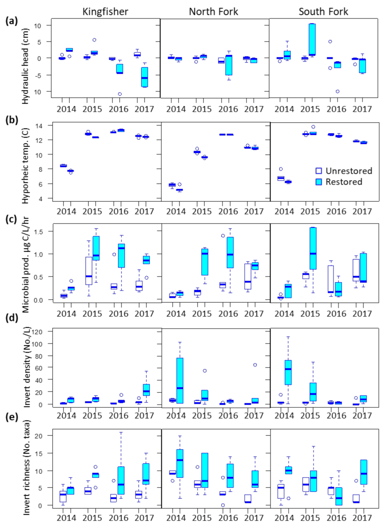
We observed differences by restoration status at two sites for temperature, one site for conductivity, and no differences for DO (reach effect p < 0.05, Supplemental Table S1). Hydraulic head within sample piezometers was consistently neutral at unrestored reaches and more dynamic at restored reaches (Figure 2a). Both hyporheic and surface water temperature in restored reaches were significantly lower than in unrestored reaches at Kingfisher and North Fork. These temperature differences diminished over time (reach x year effect, p < 0.05) (Figure 2b). Hyporheic conductivity differed by reach type only at North Fork, and was lower in the restored reach in 2016. There was no effect of reach or interaction of reach and year on surface water conductivity. Temperature, DO, and conductivity all varied over time (year effect p < 0.05) (Table S1).
Hyporheic inorganic nutrients also exhibited yearly fluctuations, but only a few differences were associated with restoration and were not consistent across sites (Supplemental Table S2). Nitrate was higher in the restored reach of Kingfisher, nitrite was lower in restored reaches of South Fork and North Fork, and total phosphorus higher in North Fork only. In contrast, differences in organic nutrient concentrations were driven more by restoration status and less by year effects. DOC was significantly higher in restored reaches of Kingfisher and North Fork, and POM was higher in restored reaches of North Fork and South Fork. We observed limited interaction effects on either organic or inorganic nutrient concentrations.
3.2. Microbes
We observed significant reach differences for microbial heterotrophic production, but little effect of restoration on bacterial abundance or microbial diversity metrics (Table 1 and Supplemental Table S3). Heterotrophic production was consistently higher in restored reaches at Kingfisher and North Fork, but not South Fork (Figure 2c). Bacterial cell abundance and the ratio of high:low nucleic acid bacteria were greater in the restored reach at Kingfisher, and planktonic H’ and evenness lower at the South Fork restored reach. Production, abundance, nucleic acid ratio, and planktonic diversity metrics all varied significantly by year, but particle-associated diversity metrics did not. We observed little to no interaction effect on any of the above variables (Table S3).
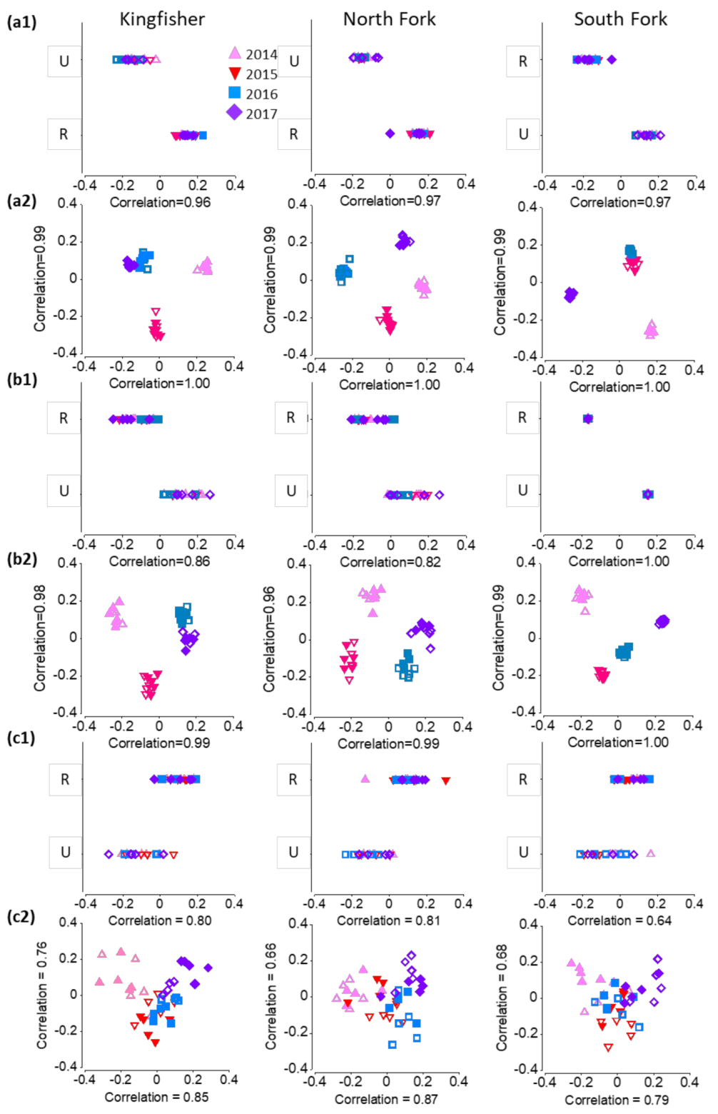
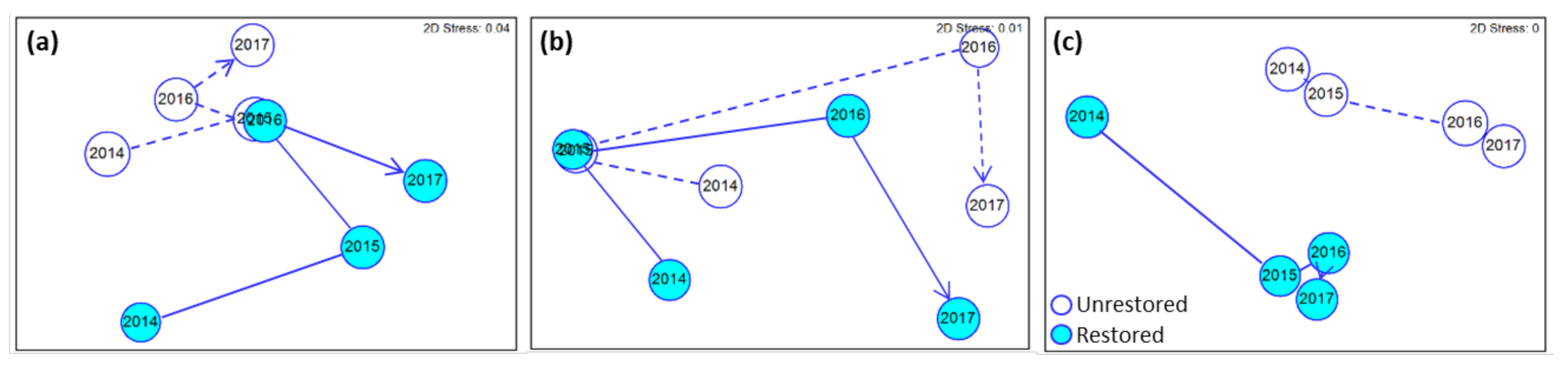
There were significant differences in microbial community structure (based on OTUs) between unrestored and restored reaches and over the years (Figure 3a,b). At each site, community structure differed significantly between restored and unrestored reaches, except in the planktonic fraction from North Fork (Table 2). Year-to-year differences in the planktonic fraction occurred at each site, but at North Fork only in the particle-associated fraction (Table 2). When all sites were combined, hyporheic communities in each fraction followed a similar time trajectory for both unrestored and restored reaches (Figure 4a,b).
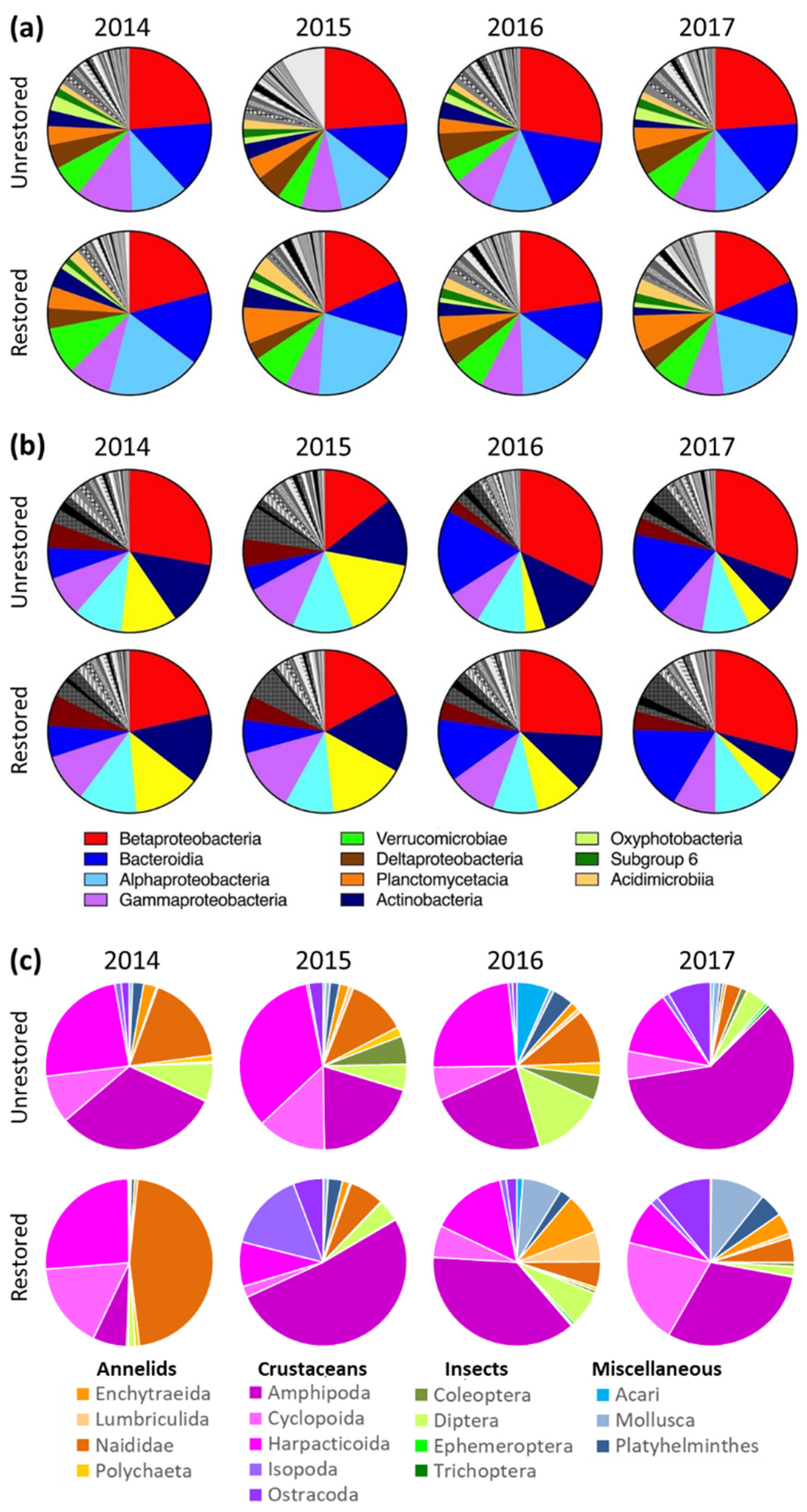
Although 98 different bacterial classes were identified in each of the two size fractions in hyporheic samples, over 75% of total microbial abundance were represented by eleven or fewer classes (Figure 5a,b). Alphaproteobacteria, Betaproteobacteria, and Bacteroidia were dominant in both size fractions; Gammaproteobacteria and Verrucomicrobiae in particle associated; and Actinobacteria and Parcubacteria in planktonic. The four most abundant particle-associated genera representing ~5% of the classified taxa at each site were Flavobacterium, Limnohabitans, Rhodoferax, and Novosphingobium (Supplemental Figure S1). In contrast, the most abundant planktonic bacterial genera varied by site. At Kingfisher, these were Limnohabitans, Polynucleobacter, and Flavobacterium. At South Fork, the top 5% included those genera plus Rickettsiella. In contrast, the most abundant bacterial genera at North Fork were hgcl clade and Limnohabitans.
In terms of taxonomic differences by reach type, Flavobacterium, Limnohabitans, Rhodoferax, and Pseudarcicella were more abundant at unrestored reaches for both size fractions (Supplemental Figures S1 and S2). Restored reaches were characterized by a higher abundance of four genera in the planktonic fraction (hgcl clade, MND1, Sulfuritalea, and Rickettsiella) and four genera in the particle-associated fraction (Novosphingobium, Bacillus, Lacihabitans, and Luteolibacter).
3.3. Invertebrates
We observed a total of 81 unique invertebrate taxa in piezometer samples collected across all reaches and years (Supplemental Table S4). Of these, 40 were unique to restored reaches, 13 unique to unrestored reaches, and 28 shared in common. Both restored and unrestored reaches were largely composed of crustaceans and annelids (Figure 5). Crustaceans made up 49–86% of total individuals at both restored and unrested reaches. Annelids contributed another 9–48% of individuals at restored reaches, and 4–21% at unrestored. Very few insects were present in either restored or unrestored reaches, with the majority from the Dipteran family Chironomidae.
Hyporheic invertebrate density and taxa richness were both significantly higher at restored than unrestored reaches across all three sites (Table 1) (Figure 2d,e). Mean invertebrate density in restored reaches averaged seven times higher than unrestored reaches, and taxa richness was double. There was also a significant interaction effect of reach and year on taxa richness at South Fork: differences between restored and unrestored reaches were greater in 2014 and 2017 relative to 2015 and 2016. The only significant year effect was at North Fork for both invertebrate density and taxa richness.
In terms of invertebrate multivariate response, both reach and year had a significant effect on taxonomic composition at every site (PERMANOVA, p < 0.05) (Table 2). We observed the least overlap between restored and unrestored reaches at North Fork, and the greatest at South Fork (Figure 3c1). Reach and year significantly interacted only at North Fork (Table 2): restored and unrestored reaches overlapped in 2014, but increasingly diverged over time. When all reaches were plotted together in multivariate space, restored reaches changed more from 2014 to 2015 than unrestored, but otherwise followed a similar time trajectory. There was little interaction between reach and year (Figure 4c).
Multivariate differences between restored and unrestored reaches was a product of higher densities and diversity of invertebrate taxa at restored reaches (Supplemental Figure S3). In particular, the annelid genera Cernosvitoviella and Pristina were more abundant in restored reaches, as were the cyclopoid copepod Acanthocyclops robustus, the harpacticoid copepod Attheyella illinoisensis, and the molluscs Pisidium and Potamopyrgus antipodarum (the highly invasive New Zealand mud snail). We observed eight unique cyclopoid species in restored reaches, but only two in unrestored. Similarly, there were 25 unique insect taxa in restored reaches compared to 17 in unrestored.
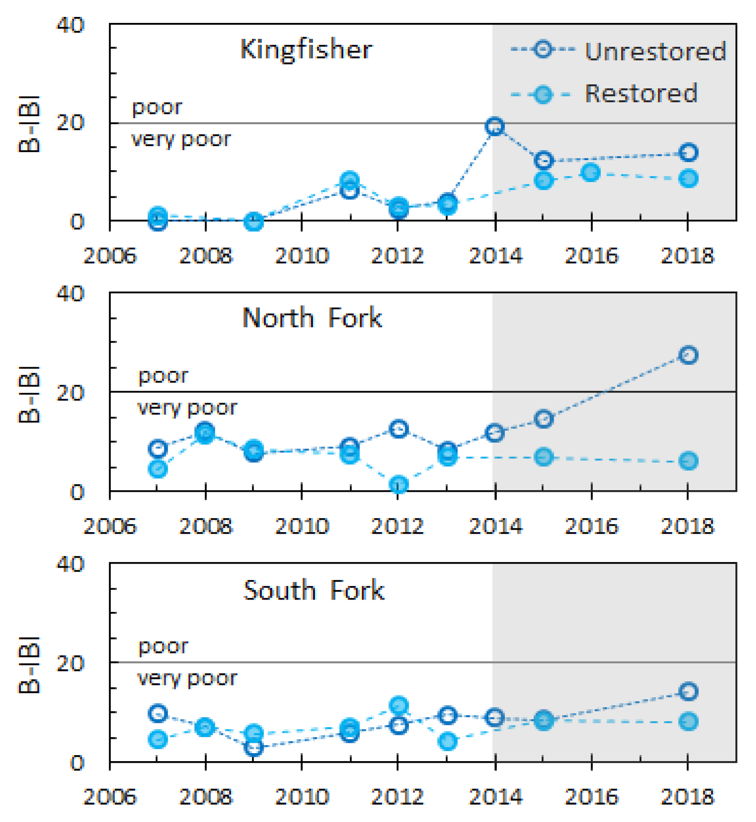
Benthic invertebrate data collected before and after restoration did not show improvements in B-IBI at any of the restored reaches (Figure 6). Prior to restoration, scores at paired unrestored and restored reaches were very similar to each other. After restoration, B-IBI increased slightly at unrestored but not at restored reaches. At Kingfisher, post-restoration B-IBI at restored reaches ranged from 0 to 9.9, while the unrestored reach increased to 12.3–19.1. At the North Fork, restored B-IBI remained near 7, while the unrestored reach steadily increased to 26.7 by 2018. At the South Fork, post-restoration B-IBI at the restored reach was 8 compared to 14.2 for the unrestored.
3.4. Relationship between Response Variables
Between six and eight environmental variables best predicted 26–45% of microbial community structure (Table 3). Hyporheic temperature and DO were common predictors across both reach types and size fractions. Differences in predictor variables between unrestored and restored reaches were greater for the particle-associated microbial fraction. Dissolved inorganic nutrients (ammonium, nitrite, phosphate) were the best predictors for unrestored reaches, and organics nutrients (DOC, POM) for restored reaches. More than half of significant predictors in the planktonic fraction were common between unrestored and restored reaches, but hyporheic silicate and bacterial abundance were stronger for unrestored reaches while DOC and hydraulic head were stronger for restored reaches.
Linear models for environmental variables prediction of invertebrate community structure had a lower fit than for microbial communities. Based on DistLM, the best fit environmental models explained only 15–18% of invertebrate community structure (Table 3). Only one predictor variable was selected for both unrestored and restored reaches: microbial production. For unrestored reaches, hyporheic DO, ammonium, nitrate and total nitrogen were significant variables. In contrast, hyporheic conductivity, hyporheic nitrite, and POM were significant predictors for invertebrate communities from restored reaches.
4. Discussion
We examined the effects of hyporheic restoration, time after restoration, and the interaction of the two on a suite of instream environmental and biological variables. The majority of biological variables we measured showed a response to restoration, as did water temperature and carbon concentrations. Given that our monitoring began immediately after project construction, we were surprised to observe little interaction effect of restoration and year. Both biological and environmental variables exhibited significant yearly variations consistent with climatic variability across our study period. A steady trend of increasing anomalously high air temperatures from 2014 to 2016 followed by a return to normal in 2017 was similar to the pattern we observed in water temperatures across all study sites [67] (Figure 2b).
Water temperature is a primary force structuring invertebrate and microbial communities [68], and strongly regulates ecological processes such as organic matter decomposition and nitrification [69]. The HZ often has a strong modulating effect on temperature in small streams [70,71]. We observed such an effect at two of our three study sites, with lower temperatures observed in restored reaches. These results are particularly noteworthy because newly planted restored reaches were largely unshaded in the three years following project construction. Given that our sampling occurred in the fall, further investigation is warranted to determine if this temperature difference increases in summer or potentially reverses in winter. Bakke et al. [35] also observed significant downstream cooling over the Kingfisher restored reach during summer baseflows, which they attributed to increased vertical water flux, subsurface flow, and hyporheic residence time.
We anticipated that increased rates of water exchange would increase hyporheic DO through aeration. However, we observed no differences in DO between restored and unrestored reaches. Increased oxygenation may have been offset by the higher level of heterotrophic production at restored reaches (Figure 2c), or by the high oxygen demand associated with microbial nitrification [72]. Another potential explanation is higher variability in hydraulic head at restored reaches (Figure 2a). Strongly upwelling areas likely contained less DO than the relatively neutral conditions observed in unrestored reaches [73]. Another importance factor to consider when interpreting project response are differences across the restoration projects themselves. Although all followed similar design principles, the full complement of hyporheic techniques was applied only at Kingfisher.
Increased hyporheic volume and residence time enhance filtration of nutrients and contaminants [41]. In the Kingfisher restored reach, Peter et al. [58] demonstrated that increased residence time significantly improved water quality: 69% of all tested organic compounds were eliminated altogether from water that spent over three hours in the HZ compared to 35% for 30 min. We observed limited restoration effect on most inorganic nutrient concentrations, but did detect differences in biologically derived nutrients. Much of the nutrient processing that occurs in the HZ is attributed to microbial metabolism, which requires DOC that comes from the breakdown of POM [74,75]. Increased channel complexity and hyporheic exchange promote the entrainment of POM into hyporheic sediments, and thus provide greater opportunity for DOC consumption via microbial metabolism [31,41,43].
Increased microbial metabolism and higher levels of DOC and POM in most of the restored reaches suggest active hyporheic nutrient processing in restored portions of Thornton Creek. Higher heterotrophic production is indicative of active metabolic processes such as nitrification/denitrification, organic material recycling, and potentially contaminant degradation [73]. The bacterial genus Novosphingobium, which was characteristic of restored reaches, is able to degrade polycyclic aromatic hydrocarbons, steroid hormones, and lignin [76,77]. In contrast, the very slow piezometer recharge rates at unrestored reaches indicates lower bioavailability of hyporheic substrates, and thus reduced opportunity for microbial metabolic activity [22,78].
Hyporheic bacterial and archaeal community structure was significantly different between restored and unrestored reaches, and differences were stronger in the particle-associated fraction (Figure 3a). One class of particle-associated bacteria that was more abundant in restored reaches was Planctomycetacia (Figure 5a). These bacteria are often involved in the initial steps of degrading large organic molecules under aerobic and anaerobic conditions in organic aggregates [79,80,81], consistent with their prominence in the particle-associated fraction. Their emergence as a dominant class in biofilters of recirculating aquaculture systems points to a significant role in organic matter degradation including anaerobic ammonium oxidation [82].
Hyporheic invertebrate density was significantly greater at all restored reaches, a finding we attribute to expanded hyporheic cross section and thus increased habitat availability. The general composition of invertebrates at both restored and unrestored reaches was typical of the HZ in that in consisting primarily of many small-bodied worms, crustaceans, mites, and some early larval stages of aquatic insects [21]. Although taxa richness was higher at all restored reaches relative to unrestored, the proportion of aquatic insects was much lower than observed at nearby forested streams (e.g., Cedar River Watershed; author’s unpublished data). The orders Ephemeroptera, Plecoptera, and Trichoptera comprised less than one percent of individuals across both restored and unrestored reaches (Figure 5c), reflective of the larger urban setting. All Thornton samples, regardless of restoration status or year, contained a high relative abundance of the disturbance-tolerant amphipod genus Crangonyx (Supplemental Figure S3).
The taxonomic shifts we observed in microbial and invertebrate hyporheic communities at restored reaches reflect local physiochemical habitat conditions in the constructed HZ [35,36]. Numerous studies have documented variability of hyporheic biota along environmental gradients that include vertical water flux, sediment characteristics, and wood density [83,84,85,86,87]. Hyporheic habitat heterogeneity at restored reaches improved with addition of large wood structures (many of which were partially or completely buried in the streambed), increased vertical water flux, and greater overall hydraulic diversity [35]. In three years of follow-up monitoring at the Kingfisher restored reach, the engineered HZ maintained a streambed of loose alluvial gravel, and did not become embedded with sand [35]. Changes in solute concentrations observed by Peter et al. [36] and the differences we observed in POM, DOC, and heterotrophic production also altered the chemical environment and food resources for hyporheic fauna.
The improvements we observed in density and taxa richness of hyporheic invertebrates between restored and unrestored reaches did not translate to the surface benthos. Across all years of the study, there was no measurable improvement in B-IBI at restored reaches (Figure 6). Invertebrates are sensitive to a variety of urban stressors, expressed at both large and small spatial scales [49]. This was reinforced by the relatively low amount of variability we were able to explain in hyporheic invertebrate composition with the suite of environmental data collected in this study (Table 3). While these floodplain reconnection projects had measurable local impacts, they cannot address all limiting factors operating across the entire urban watershed. In Thornton Creek, these include (but are not limited to) poor water quality, invasive species, lack of source populations for recolonization, and a highly modified hydrologic regime [44,88].
5. Conclusions
Floodplain reconnection is a green infrastructure approach that benefits both stormwater management and urban stream restoration. Engineered streambeds with a constructed HZ are an extension of this tool that further enhance connectivity through surface and subsurface exchange. [34]. This technique has already been shown to improve water quality, decrease stream summer water temperature, increase hyporheic residence time, and improve hydraulic habitat diversity at one project site on Thornton Creek [35,36]. We expanded upon these studies by examining project response across three sites, and found evidence of fall water temperature modulation; increased POM and DOC concentrations; higher heterotrophic production; shifts in microbial taxonomic composition; and increased hyporheic invertebrate density and richness. We did not detect changes in hyporheic DO. Nor were we able to predict a high degree of microbial or invertebrate community structure with the environmental variables measured in this study. Project monitoring results reflect complex feedback loops between chemical, physical, and biological processes operating within the HZ [73].
We are not aware of any published studies that have examined biological response within the HZ to restoration. In general, there is very little literature on biological processes of urban HZ’s, and even less in relation to stream restoration [41,75,89]. This information gap merits further inquiry. In particular, it will be important to examine how fish and other stream organisms respond to hyporheic restoration, examine response over different seasons and climatic conditions, and explore potential constraints on recolonization by invertebrates and other less-mobile organisms [90]. Based on what we and others have observed thus far, these pilot projects offer multiple benefits to cities: enhanced floodplain storage of water, wood, and sediment; contaminant removal; urban greenspaces; and improved stream health. Rebuilding watershed connectivity through GSI and process-based restoration is a blueprint that can be applied throughout the world to build more resilient cities and healthier streams. In the fall of 2018, Chinook salmon (O. tshawytscha) spawned in Thornton Creek for the first time in at least eight years, building their redd atop the new streambed and its restored HZ [35].
Supplementary Materials
The following are available online at https://www.mdpi.com/2073-4441/13/4/481/s1, Figure S1. Shade plot of averaged abundances for higher-abundance bacterial genera from the particle-associated fraction of hyporheic water; Figure S2. Shade plot of averaged abundances for higher-abundance bacterial genera from the planktonic fraction of hyporheic water; Figure S3. Shade plot of mean invertebrate density for taxa that contributed at least 1% of total abundances across all years and reaches; Table S1. Environmental data means and (standard deviations) by year and reach, with results of two-way fixed effects crossed ANOVA; Table S2. Nutrient data means and standard deviations by year and reach, with results of two-way fixed effects crossed ANOVA; Table S3. Microbial data means and (standard deviations) by year and reach, with results of two-way fixed effects crossed ANOVA; Table S4. List of all invertebrate taxa observed in piezometer samples from unrestored (U) and restored (R) reaches across all sample years (2014–2017).
Author Contributions
Conceptualization, S.A.M., L.D.R., A.E.B. and K.D.L.; methodology, S.A.M., L.D.R., A.E.B., G.W.G. and A.H.W.; software, G.W.G.; formal analysis, S.A.M., L.D.R., A.E.B. and A.H.W.; investigation, S.A.M., L.D.R. and A.E.B.; data curation, S.A.M. and L.D.R.; writing—original draft preparation, S.A.M. and L.D.R.; writing—review and editing, S.A.M., L.D.R., A.E.B., A.H.W. and K.D.L.; visualization, S.A.M. and L.D.R.; funding acquisition, K.D.L. All authors have read and agreed to the published version of the manuscript.
Funding
This research was funded by the City of Seattle, Agreements 14-077-A and 17 122-A.
Institutional Review Board Statement
Scientific collection permits for this study were obtained prior to field collections, and were issued by the Washington Department of Fish and Wildlife. All sampling and handling of invertebrates was carried out in accordance with permit conditions.
Informed Consent Statement
Not applicable.
Data Availability Statement
Data presented in this study are openly available in Morley et al. [91].
Acknowledgments
From NOAA’s Northwest Fisheries Science Center we thank Paul Hoppe, William Nilsson, Karrie Hanson, and Karl Veggerby for field assistance; Su Kim, Britta Timpane-Padgham, and Oleksander Stefankiv for figure preparation; Martin Liermann for statistical consultation, and Karrie Hanson and Gabe Wisswaesser for technical editing. From USFWS we thank Paul Bakke for piezometer consultation and design. From Seattle Public Utilities we thank Chapin Pier and Steve Damm for logistical support. From King County DNRP we thank Kate Macneale and the bug crew for benthic invertebrate sampling. Invertebrate samples were processed by Rhithron Associates. We thank Stuart Munsch, Britta Timpane-Padgham, George Pess, and two anonymous reviewers for their thoughtful comments on earlier versions of this manuscript.
Conflicts of Interest
The funders had no role in the design of the study; in the collection, analyses, or interpretation of data; or in the decision to publish the results.
References
- Walsh, C.J.; Booth, D.B.; Burns, M.J.; Fletcher, T.D.; Hale, R.L.; Hoang, L.N.; Livingston, G.; Rippy, M.A.; Roy, A.H.; Scoggins, M. Principles for urban stormwater management to protect stream ecosystems. Freshw. Sci. 2016, 35, 398–411. [Google Scholar] [CrossRef] [Green Version]
- Levin, P.S.; Howe, E.R.; Robertson, J.C. Impacts of stormwater on coastal ecosystems: The need to match the scales of management objectives and solutions. Philos. Trans. R. Soc. B 2020, 375, 20190460. [Google Scholar] [CrossRef]
- Shuster, W.D.; Bonta, J.; Thurston, H.; Warnemuende, E.; Smith, D. Impacts of impervious surface on watershed hydrology: A review. Urban Water J. 2005, 2, 263–275. [Google Scholar] [CrossRef]
- Elmore, A.J.; Kaushal, S.S. Disappearing headwaters: Patterns of stream burial due to urbanization. Front. Ecol. Environ. 2008, 6, 308–312. [Google Scholar] [CrossRef]
- McGrane, S.J. Impacts of urbanisation on hydrological and water quality dynamics, and urban water management: A review. Hydrol. Sci. J. 2016, 61, 2295–2311. [Google Scholar] [CrossRef]
- Tian, Z.; Zhao, H.; Peter, K.T.; Gonzalez, M.; Wetzel, J.; Wu, C.; Hu, X.; Prat, J.; Mudrock, E.; Hettinger, R. A ubiquitous tire rubber–derived chemical induces acute mortality in coho salmon. Science 2020, 371, 185–189. [Google Scholar] [CrossRef]
- Walsh, C.J.; Roy, A.H.; Feminella, J.W.; Cottingham, P.D.; Groffman, P.M.; Morgan, R.P. The urban stream syndrome: Current knowledge and the search for a cure. J. N. Am. Benthol. Soc. 2005, 24, 706–723. [Google Scholar] [CrossRef]
- Dhakal, K.P.; Chevalier, L.R. Urban stormwater governance: The need for a paradigm shift. Environ. Manag. 2016, 57, 1112–1124. [Google Scholar] [CrossRef]
- Prudencio, L.; Null, S.E. Stormwater management and ecosystem services: A review. Environ. Res. Lett. 2018, 13, 033002. [Google Scholar] [CrossRef]
- Yang, B.; Li, S. Green infrastructure design for stormwater runoff and water quality: Empirical evidence from large watershed-scale community developments. Water 2013, 5, 2038–2057. [Google Scholar] [CrossRef]
- McIntyre, J.; Davis, J.; Hinman, C.; Macneale, K.; Anulacion, B.; Scholz, N.; Stark, J. Soil bioretention protects juvenile salmon and their prey from the toxic impacts of urban stormwater runoff. Chemosphere 2015, 132, 213–219. [Google Scholar] [CrossRef] [Green Version]
- Ward, J.; Tockner, K.; Schiemer, F. Biodiversity of floodplain river ecosystems: Ecotones and connectivity1. River Res. Appl. 1999, 15, 125–139. [Google Scholar] [CrossRef]
- Opperman, J.J.; Luster, R.; McKenney, B.A.; Roberts, M.; Meadows, A.W. Ecologically functional floodplains: Connectivity, flow regime, and scale 1. JAWRA J. Am. Water Resour. Assoc. 2010, 46, 211–226. [Google Scholar] [CrossRef]
- Dixon, S.J.; Sear, D.A.; Odoni, N.A.; Sykes, T.; Lane, S.N. The effects of river restoration on catchment scale flood risk and flood hydrology. Earth Surface Process. Landf. 2016, 41, 997–1008. [Google Scholar] [CrossRef]
- Ahilan, S.; Guan, M.; Sleigh, A.; Wright, N.; Chang, H. The influence of floodplain restoration on flow and sediment dynamics in an urban river. J. Flood Risk Manag. 2018, 11, S986–S1001. [Google Scholar] [CrossRef]
- O’Donnell, E.C.; Thorne, C.R.; Yeakley, J.A.; Chan, F.K.S. Sustainable flood risk and stormwater management in blue-green cities; an interdisciplinary case study in Portland, Oregon. JAWRA J. Am. Water Resour. Assoc. 2020, 56, 757–775. [Google Scholar] [CrossRef]
- Beechie, T.J.; Sear, D.A.; Olden, J.D.; Pess, G.R.; Buffington, J.M.; Moir, H.; Roni, P.; Pollock, M.M. Process-based principles for restoring river ecosystems. BioScience 2010, 60, 209–222. [Google Scholar] [CrossRef] [Green Version]
- Vietz, G.J.; Rutherfurd, I.D.; Fletcher, T.D.; Walsh, C.J. Thinking outside the channel: Challenges and opportunities for protection and restoration of stream morphology in urbanizing catchments. Landsc. Urban Plan 2016, 145, 34–44. [Google Scholar] [CrossRef]
- Wohl, E. Connectivity in rivers. Progress Phys. Geogr. 2017, 41, 345–362. [Google Scholar] [CrossRef]
- Orghidan, T. Ein neuer Lebensraum des unterirdischen Wassers, der hyporheische Biotop. Arch. Hydrobiol. 1959, 55, 392–414. [Google Scholar]
- Boulton, A.J.; Findlay, S.; Marmonier, P.; Stanley, E.H.; Valett, H.M. The functional significance of the hyporheic zone in streams and rivers. Annu. Rev. Ecol. Syst. 1998, 29, 59–81. [Google Scholar] [CrossRef] [Green Version]
- Fischer, H.; Kloep, F.; Wilzcek, S.; Pusch, M.T. A river’s liver—Microbial processes within the hyporheic zone of a large lowland river. Biogeochemistry 2005, 76, 349–371. [Google Scholar] [CrossRef]
- Hancock, P.J.; Boulton, A.J.; Humphreys, W.F. Aquifers and hyporheic zones: Towards an ecological understanding of groundwater. Hydrogeol. J. 2005, 13, 98–111. [Google Scholar] [CrossRef]
- Lewandowski, J.; Arnon, S.; Banks, E.; Batelaan, O.; Betterle, A.; Broecker, T.; Coll Mora, C.; Drummond, J.; Gaona, J.; Galloway, J.; et al. Is the Hyporheic Zone Relevant beyond the Scientific Community? Water 2019, 11, 2230. [Google Scholar] [CrossRef] [Green Version]
- Robertson, A.L.; Wood, P.J. Ecology of the hyporheic zone: Origins, current knowledge and future directions. Fundam. Appl. Limnol. 2010, 176, 279–289. [Google Scholar] [CrossRef]
- Vorste, R.V.; Corti, R.; Sagouis, A.; Datry, T. Invertebrate communities in gravel-bed, braided rivers are highly resilient to flow intermittence. Freshw. Sci. 2016, 35, 164–177. [Google Scholar] [CrossRef] [Green Version]
- Stanford, J.A.; Ward, J.V. The Hyporheic Habitat of River Ecosystems. Nature 1988, 335, 64–66. [Google Scholar] [CrossRef]
- Gilbert, J.; Doleolivier, M.J.; Marmonier, P.; Vervier, P. Surface Water-Groundwater Ecotones. Ecol. Manag. Aquat. Terr. Ecotones 1990, 4, 199–225. [Google Scholar]
- Boulton, A.J. Hyporheic rehabilitation in rivers: Restoring vertical connectivity. Freshw. Biol. 2007, 52, 632–650. [Google Scholar] [CrossRef]
- Kasahara, T.; Datry, T.; Mutz, M.; Boulton, A.J. Treating causes not symptoms: Restoration of surface-groundwater interactions in rivers. Mar. Freshw. Res. 2009, 60, 976–981. [Google Scholar] [CrossRef]
- Hester, E.T.; Gooseff, M.N. Moving Beyond the Banks: Hyporheic Restoration Is Fundamental to Restoring Ecological Services and Functions of Streams. Environ. Sci. Technol. 2010, 44, 1521–1525. [Google Scholar] [CrossRef]
- Mendoza-Lera, C.; Datry, T. Relating hydraulic conductivity and hyporheic zone biogeochemical processing to conserve and restore river ecosystem services. Sci. Total Environ. 2017, 579, 1815–1821. [Google Scholar] [CrossRef]
- Magliozzi, C.; Coro, G.; Grabowski, R.C.; Packman, A.I.; Krause, S. A multiscale statistical method to identify potential areas of hyporheic exchange for river restoration planning. Environ. Model. Softw. 2019, 111, 311–323. [Google Scholar] [CrossRef] [Green Version]
- Herzog, S.P.; Higgins, C.P.; McCray, J.E. Engineered Streambeds for Induced Hyporheic Flow: Enhanced Removal of Nutrients, Pathogens, and Metals from Urban Streams. J. Environ. Eng. 2015, 142, 04015053. [Google Scholar] [CrossRef]
- Bakke, P.D.; Hrachovec, M.; Lynch, K.D. Hyporheic Process Restoration: Design and Performance of an Engineered Streambed. Water 2020, 12, 425. [Google Scholar] [CrossRef] [Green Version]
- Peter, K.T.; Herzog, S.; Tian, Z.Y.; Wu, C.; McCray, J.E.; Lynch, K.; Kolodziej, E.P. Evaluating emerging organic contaminant removal in an engineered hyporheic zone using high resolution mass spectrometry. Water Res. 2019, 150, 140–152. [Google Scholar] [CrossRef]
- Crispell, J.K.; Endreny, T.A. Hyporheic exchange flow around constructed in-channel structures and implications for restoration design. Hydrol. Process. 2009, 23, 1158–1168. [Google Scholar] [CrossRef]
- Knust, A.E.; Warwick, J.J. Using a fluctuating tracer to estimate hyporheic exchange in restored and unrestored reaches of the Truckee River, Nevada, USA. Hydrol. Process. 2009, 23, 1119–1130. [Google Scholar] [CrossRef]
- Peralta-Maraver, I.; Perkins, D.M.; Thompson, M.S.; Fussmann, K.; Reiss, J.; Robertson, A.L. Comparing biotic drivers of litter breakdown across stream compartments. J. Anim. Ecol. 2019, 88, 1146–1157. [Google Scholar] [CrossRef]
- Weatherill, J.J.; Atashgahi, S.; Schneidewind, U.; Krause, S.; Ullah, S.; Cassidy, N.; Rivett, M.O. Natural attenuation of chlorinated ethenes in hyporheic zones: A review of key biogeochemical processes and in-situ transformation potential. Water Res. 2018, 128, 362–382. [Google Scholar] [CrossRef] [Green Version]
- Lawrence, J.E.; Skold, M.E.; Hussain, F.A.; Silverman, D.R.; Resh, V.H.; Sedlak, D.L.; Luthy, R.G.; McCray, J.E. Hyporheic Zone in Urban Streams: A Review and Opportunities for Enhancing Water Quality and Improving Aquatic Habitat by Active Management. Environ. Eng. Sci. 2013, 30, 480–501. [Google Scholar] [CrossRef]
- Grimm, N.B.; Baxter, C.V.; Crenshaw, C.L. Surface-subsurface interactions in streams. In Methods in Stream Ecology; Hauer, F.R., Lamberti, G.A., Eds.; Academic Press: San Diego, CA, USA, 2007; pp. 761–782. [Google Scholar]
- Drummond, J.; Aubeneau, A.; Packman, A. Stochastic modeling of fine particulate organic carbon dynamics in rivers. Water Resour. Res. 2014, 50, 4341–4356. [Google Scholar] [CrossRef]
- City of Seattle. State of the Waters. In Volume I: Seattle Watercourses; City of Seattle: Seattle, WA, USA, 2007; Volume I, p. 262. Available online: https://www.seattle.gov/util/cs/groups/public/@spu/@conservation/documents/webcontent/spu01_003413.pdf (accessed on 4 November 2020).
- Alberti, M.; Booth, D.; Hill, K.; Coburn, B.; Avolio, C.; Coe, S.; Spirandelli, D. The impact of urban patterns on aquatic ecosystems: An empirical analysis in Puget lowland sub-basins. Landsc. Urban Plan. 2007, 80, 345–361. [Google Scholar] [CrossRef]
- Brett, M.T.; Arhonditsis, G.B.; Mueller, S.E.; Hartley, D.M.; Frodge, J.D.; Funke, D.E. Non-point-source impacts on stream nutrient concentrations along a forest to urban gradient. Environ. Manag. 2005, 35, 330–342. [Google Scholar] [CrossRef] [PubMed]
- Reidy, C. Variability of Hyporheic Zones in Puget Sound Lowland Streams; University of Washington: Seattle, WA, USA, 2004. [Google Scholar]
- Scholz, N.L.; Myers, M.S.; McCarthy, S.G.; Labenia, J.S.; McIntyre, J.K.; Ylitalo, G.M.; Rhodes, L.D.; Laetz, C.A.; Stehr, C.M.; French, B.L.; et al. Recurrent Die-Offs of Adult Coho Salmon Returning to Spawn in Puget Sound Lowland Urban Streams. PLoS ONE 2011, 6, e28013. [Google Scholar] [CrossRef]
- Morley, S.A.; Karr, J.R. Assessing and restoring the health of urban streams in the Puget Sound basin. Conserv. Biol. 2002, 16, 1498–1509. [Google Scholar] [CrossRef] [Green Version]
- Puget Sound Stream Benthos. Available online: https://pugetsoundstreambenthos.org/ (accessed on 11 April 2020).
- Valderrama, J.C. The simultaneous analysis of total nitrogen and total phosphorus in natural waters. Mar. Chem. 1981, 10, 109–122. [Google Scholar] [CrossRef]
- Scientific Committee on Oceanic Research. Protocols for the Joint Global Ocean Flux Study (JGOFS) Core Measurements; Intergovernmental Oceanographic Commission: Paris, France, 1994; Volume 29, p. 170. [Google Scholar]
- Hambrook Berkman, J.A.; Canova, M.G. Algal Biomass Indicators (ver.1.0): U.S. Geological Survey Techniques of Water Resources Investigations; Book 9, Chapter A7, Section 7.4; U.S. Geological Survey: Reston, VA, USA, 2007. [CrossRef]
- Longnecker, K.; Sherr, B.F.; Sherr, E.B. Variation in cell-specific rates of leucine and thymidine incorporation by marine bacteria with high and with low nucleic acid content off the Oregon coast. Aquat. Microb. Ecol. 2006, 43, 113–125. [Google Scholar] [CrossRef]
- Sherr, E.B.; Sherr, B.F.; Longnecker, K. Distribution of bacterial abundance and cell-specific nucleic acid content in the Northeast Pacific Ocean. Deep Sea Res. Part 1 2006, 53, 713–725. [Google Scholar] [CrossRef]
- Green, M.R.; Sambrook, J. Isolation of High-Molecular-Weight DNA from Suspension Cultures of Mammalian Cells Using Proteinase K and Phenol. Cold Spring Harb. Protoc. 2018, 2018. [Google Scholar] [CrossRef]
- Illumina. 16S Metagenomic Sequencing Library Preparation; Illumina: San Diego, CA, USA, 2013. [Google Scholar]
- Bolyen, E.; Rideout, J.R.; Dillon, M.R.; Bokulich, N.A.; Abnet, C.C.; Al-Ghalith, G.A.; Alexander, H.; Alm, E.J.; Arumugam, M.; Asnicar, F.; et al. Author Correction: Reproducible, interactive, scalable and extensible microbiome data science using QIIME 2. Nat. Biotechnol. 2019, 37, 1091. [Google Scholar] [CrossRef] [PubMed]
- Quast, C.; Pruesse, E.; Yilmaz, P.; Gerken, J.; Schweer, T.; Yarza, P.; Peplies, J.; Glockner, F.O. The SILVA ribosomal RNA gene database project: Improved data processing and web-based tools. Nucleic Acids Res. 2013, 41, D590–D596. [Google Scholar] [CrossRef] [PubMed]
- Yilmaz, P.; Parfrey, L.W.; Yarza, P.; Gerken, J.; Pruesse, E.; Quast, C.; Schweer, T.; Peplies, J.; Ludwig, W.; Glockner, F.O. The SILVA and “All-species Living Tree Project (LTP)” taxonomic frameworks. Nucleic Acids Res. 2014, 42, D643–D648. [Google Scholar] [CrossRef] [Green Version]
- Pruesse, E.; Peplies, J.; Glöckner, F.O. SINA: Accurate high-throughput multiple sequence alignment of ribosomal RNA genes. Bioinformatics 2012, 28, 1823–1829. [Google Scholar] [CrossRef]
- Clarke, K.R.; Gorley, R.N. PRIMER v6: User Manual/Tutorial; PRIMER-E: Plymouth, UK, 2006. [Google Scholar]
- Leavy, T.R.; Bakke, P.; Peters, R.J.; Morley, S.A. Influence of Habitat Complexity and Floodplain Reconnection Projects on the Physical and Biological Conditions of Seattle Urban Streams: Pre Project Monitoring, 2005–2009; U.S. Fish and Wildlife Service, Western Washington Fish and Wildlife Office: Lacey, WA, USA, 2010.
- Morley, S.A.; Hall, J.E.; Chamberlin, J.W.; Hanson, K. Thornton Creek Restoration: Baseline Project Effectiveness Monitoring, 2012–2013; Report of the National Marine Fisheries Service to the City of Seattle; Department of Public Utilities: Seattle, WA, USA, 2013.
- R Foundation for Statistical Computing. R: A Language and Environment for Statistical Computing; R Foundation for Statistical Computing: Vienna, Austria, 2019. [Google Scholar]
- Anderson, M.J.; Gorley, R.N.; Clarke, K.R. PERMANOVA+ for PRIMER: Guide to Software and Statistical Methods; PRIMER-E: Plymouth, UK, 2008. [Google Scholar]
- Puget Sound Ecosystem Monitoring Program Marine Waters Workgroup. Puget Sound Marine Waters 2017 Overview; Moore, S.K., Wold, R., Stark, K., Bos, J., Williams, P., Hamel, N., Kim, S., Brown, A., Krembs, C., Newton, J., Eds.; Available online: https://www.psp.wa.gov/PSmarinewatersoverview.php (accessed on 11 April 2020).
- Gaudes, A.; Artigas, J.; Romani, A.; Sabater, S.; Munoz, I. Contribution of microbial and invertebrate communities to leaf litter colonization in a Mediterranean stream. J. N. Am. Benthol. Soc. 2009, 28, 34–43. [Google Scholar] [CrossRef] [Green Version]
- Krause, S.; Hannah, D.M.; Fleckenstein, J.H.; Heppell, C.M.; Kaeser, D.; Pickup, R.; Pinay, G.; Robertson, A.L.; Wood, P.J. Inter-disciplinary perspectives on processes in the hyporheic zone. Ecohydrology 2011, 4, 481–499. [Google Scholar] [CrossRef] [Green Version]
- Story, A.; Moore, R.D.; Macdonald, J.S. Stream temperatures in two shaded reaches below cutblocks and logging roads: Downstream cooling linked to subsurface hydrology. Can. J. For. Res. 2003, 33, 1383–1396. [Google Scholar] [CrossRef] [Green Version]
- Hannah, D.M.; Malcolm, I.A.; Soulsby, C.; Youngson, A.F. Heat exchanges and temperatures within a salmon spawning stream in the cairngorms, Scotland: Seasonal and sub-seasonal dynamics. River Res. Appl. 2004, 20, 635–652. [Google Scholar] [CrossRef]
- Storey, R.G.; Fulthorpe, R.R.; Williams, D.D. Perspectives and predictions on the microbial ecology of the hyporheic zone. Freshw. Biol. 1999, 41, 119–130. [Google Scholar] [CrossRef] [Green Version]
- Peralta-Maraver, I.; Reiss, J.; Robertson, A.L. Interplay of hydrology, community ecology and pollutant attenuation in the hyporheic zone. Sci. Total Environ. 2018, 610, 267–275. [Google Scholar] [CrossRef] [Green Version]
- Duff, J.; Triska, F. Nitrogen Biogeochemistry and Surface–Subsurface Exchange in Streams. In Streams and Ground Waters; Academic Press: San Diego, CA, USA, 2000; pp. 197–220. [Google Scholar] [CrossRef]
- Merill, L.; Tonjes, D.J. A Review of the Hyporheic Zone, Stream Restoration, and Means to Enhance Denitrification. Crit. Rev. Environ. Sci. Technol. 2014, 44, 2337–2379. [Google Scholar] [CrossRef]
- Ohta, Y.; Nishi, S.; Hasegawa, R.; Hatada, Y. Combination of six enzymes of a marine Novosphingobium converts the stereoisomers of β-O-4 lignin model dimers into the respective monomers. Sci. Rep. 2015, 5, 15105. [Google Scholar] [CrossRef]
- Chen, Y.-L.; Fu, H.-Y.; Lee, T.-H.; Shih, C.-J.; Huang, L.; Wang, Y.-S.; Ismail, W.; Chiang, Y.-R. Estrogen degraders and estrogen degradation pathway identified in an activated sludge. Appl. Environ. Microb. 2018, 84. [Google Scholar] [CrossRef] [Green Version]
- Wagner, K.; Bengtsson, M.M.; Besemer, K.; Sieczko, A.; Burns, N.R.; Herberg, E.R.; Battin, T.J. Functional and Structural Responses of Hyporheic Biofilms to Varying Sources of Dissolved Organic Matter. Appl. Environ. Microb. 2014, 80, 6004–6012. [Google Scholar] [CrossRef] [Green Version]
- DeLong, E.F.; Franks, D.G.; Alldredge, A.L. Phylogenetic diversity of aggregate-attached vs. free-living marine bacterial assemblages. Limnol. Oceanogr. 1993, 38, 924–934. [Google Scholar] [CrossRef] [Green Version]
- Fuchsman, C.A.; Staley, J.T.; Oakley, B.B.; Kirkpatrick, J.B.; Murray, J.W. Free-living and aggregate-associated Planctomycetes in the Black Sea. FEMS Microbiol. Ecol. 2012, 80, 402–416. [Google Scholar] [CrossRef] [PubMed]
- Glöckner, F.O.; Kube, M.; Bauer, M.; Teeling, H.; Lombardot, T.; Ludwig, W.; Gade, D.; Beck, A.; Borzym, K.; Heitmann, K. Complete genome sequence of the marine planctomycete Pirellula sp. strain 1. Proc. Natl. Acad. Sci. USA 2003, 100, 8298–8303. [Google Scholar] [CrossRef] [Green Version]
- Zhu, P.; Ye, Y.; Pei, F.; Lu, K. Characterizing the structural diversity of a bacterial community associated with filter materials in recirculating aquaculture systems of Scortum barcoo. Can. J. Microbiol. 2012, 58, 303–310. [Google Scholar] [CrossRef]
- Sliva, L.; Williams, D.D. Responses of hyporheic meiofauna to habitat manipulation. Hydrobiologia 2005, 548, 217–232. [Google Scholar] [CrossRef]
- Boulton, A.J.; Datry, T.; Kasahara, T.; Mutz, M.; Stanford, J.A. Ecology and management of the hyporheic zone: Stream-groundwater interactions of running waters and their floodplains. J. N. Am. Benthol. Soc. 2010, 29, 26–40. [Google Scholar] [CrossRef] [Green Version]
- Descloux, S.; Datry, T.; Usseglio-Polatera, P. Trait-based structure of invertebrates along a gradient of sediment colmation: Benthos versus hyporheos responses. Sci. Total Environ. 2014, 466, 265–276. [Google Scholar] [CrossRef]
- Wagenhoff, A.; Olsen, D. Does large woody debris affect the hyporheic ecology of a small New Zealand pasture stream? N. Zeal. J. Mar. Freshw. 2014, 48, 547–559. [Google Scholar] [CrossRef]
- Magliozzi, C.; Usseglio-Polatera, P.; Meyer, A.; Grabowski, R.C. Functional traits of hyporheic and benthic invertebrates reveal importance of wood-driven geomorphological processes in rivers. Funct. Ecol. 2019, 33, 1758–1770. [Google Scholar] [CrossRef]
- Sundermann, A.; Stoll, S.; Haase, P. River restoration success depends on the species pool of the immediate surroundings. Ecol. Appl. 2011, 21, 1962–1971. [Google Scholar] [CrossRef] [PubMed]
- Hester, E.T.; Gooseff, M.N. Hyporheic restoration in streams and rivers. In Stream Restoration in Dynamic Fluvial Systems: Scientific Approaches, Analyses, and Tools; Simon, A., Bennett, S., Castro, J., Eds.; American Geophysical Union: Washington, DC, USA, 2011; Volume 194. [Google Scholar]
- Blakely, T.J.; Harding, J.S.; McIntosh, A.R.; Winterbourn, M.J. Barriers to the recovery of aquatic insect communities in urban streams. Freshw. Biol. 2006, 51, 1634–1645. [Google Scholar] [CrossRef]
- Morley, S.A.; Rhodes, L.D.; Baxter, A.E.; Goetz, G.W.; Wells, A.H.; Lynch, K.D. Invertebrate, Microbial, and Environmental Data from Surface and Hyporheic Waters of Urban and Forested Streams of the Cedar River-Lake Washington Watershed; NOAA Data Report NMFS-NWFSC-DR-2021; U.S. Department of Commerce: Washington, DC, USA, 2021. [CrossRef]
Figure 1.
Locations of restored and unrestored study reaches within the Kingfisher and Confluence (North Fork and South Fork) floodplain restoration projects on Thornton Creek, in the NE quadrant of the City of Seattle. Inset map shows location of Seattle within Washington State, USA.
Figure 1.
Locations of restored and unrestored study reaches within the Kingfisher and Confluence (North Fork and South Fork) floodplain restoration projects on Thornton Creek, in the NE quadrant of the City of Seattle. Inset map shows location of Seattle within Washington State, USA.

Figure 2.
Boxplots of univariate response metrics plotted by site, restoration status, and year for (a) hydraulic head (b), hyporheic temperature (c) microbial heterotrophic production (d) hyporheic invertebrate density, and (e) hyporheic invertebrate taxa richness.
Figure 2.
Boxplots of univariate response metrics plotted by site, restoration status, and year for (a) hydraulic head (b), hyporheic temperature (c) microbial heterotrophic production (d) hyporheic invertebrate density, and (e) hyporheic invertebrate taxa richness.

Figure 3.
Community composition of (a) particle-associated microbes, (b) planktonic microbes, and (c) invertebrates plotted using canonical correlation to maximize separation by 1. restoration status and 2. year; U = unrestored (outlined symbols), R = restored (filled symbols). For all plots, points closer together are more similar in composition. Axes are labeled with their respective canonical correlation values. Microbe taxonomy is based on standardized log transformed OTU abundances and invertebrate on fourth root-transformed numerical density.

Figure 4.
Non-metric multidimensional scaling of reach centroids averaged across all sites for (a) particle-associated microbes, (b) planktonic microbes, and (c) invertebrates. Lines represent direction of change by year; circles are proportional to within-group multivariate dispersion (i.e., mean distance of individual samples to the centroid). Microbial composition is standardized log transformed OTU abundances and invertebrates fourth root-transformed numerical density.

Figure 5.
Taxonomic composition across all sites plotted by year and restoration status as relative abundance of (a) particle-associated bacteria, (b) planktonic bacteria, and (c) invertebrates. For bacteria, only classes contributing to >75% cumulative relative abundance are shown.
Figure 5.
Taxonomic composition across all sites plotted by year and restoration status as relative abundance of (a) particle-associated bacteria, (b) planktonic bacteria, and (c) invertebrates. For bacteria, only classes contributing to >75% cumulative relative abundance are shown.

Figure 6.
Benthic-Index of Biology Integrity (B-IBI) scores at restored and unrestored reaches for each study site. B-IBI values of 0–19 = very poor, 20–39 = poor, 40–59 = fair, 60–79 = good, and 80–100 = excellent. Construction at restoration sites was completed in November of 2014; post-restoration data are highlighted in grey. B-IBI data were collected by King County on behalf of Seattle Public Utilities and is publicly available at www.pugetsoundstreambenthos.org (accessed on 10 February 2021).


Table 1.
Microbial and invertebrate diversity and density ANOVA results by reach, year, and interaction of reach and year. Significant differences by reach are designated as “>” or “<”; “ns” indicates p > 0.05; U = unrestored reach, and R = restored reach; KF = Kingfisher, NF = North Fork, and SF = South Fork. Differences by year are indicated with superscripted letters, and increasing values are arranged from left to right. Years with shared letters are not significantly different (p > 0.05). “-” indicates there was no interaction effect of reach and year. Microbial metrics are based on OTUs in the planktonic fraction of hyporheic samples. Invertebrate density was log transformed and taxa richness square root transformed.
| Variable | Site | n | Reach | Year | 2014 | 2015 | 2016 | 2017 |
|---|---|---|---|---|---|---|---|---|
| Microbial diversity (H’) | KF | 40 | ns | 2014 a, 2015 a, 2016 b, 2017 c | - | - | - | - |
| NF | 39 | ns | 2015 a, 2014 ab, 2016 ab, 2017 c | - | - | - | - | |
| SF | 40 | U > R | 2015 a, 2014 ab, 2016 b, 2017 c | - | - | - | - | |
| Microbial richness (d) | KF | 40 | ns | 2014 a, 2015 a, 2017 b, 2016 c | - | - | - | - |
| NF | 39 | ns | 2015 a, 2014 ab, 2016 b, 2017 b | - | - | - | - | |
| SF | 40 | U > R | 2015 a, 2014 b, 2017 c, 2016 c | ns | ns | U > R | ns | |
| Microbial evenness (J) | KF | 40 | ns | 2016 a, 2014 b, 2015 b, 2017 b | - | - | - | - |
| NF | 39 | ns | ns | - | - | - | - | |
| SF | 40 | ns | 2016 a, 2014 ab, 2015 b, 2017 c | - | - | - | - | |
| Invertebrate density (No L−1) | KF | 40 | R > U | ns | - | - | - | - |
| NF | 40 | R > U | 2017 a, 2016 a, 2015 ab, 2014 b | - | - | - | - | |
| SF | 39 | R > U | ns | - | - | - | - | |
| Invertebrate richness (No. taxa) | KF | 40 | R > U | ns | - | - | - | - |
| NF | 40 | R > U | 2017 a, 2016 ab, 2015 ab, 2014 b | - | - | - | - | |
| SF | 39 | R > U | ns | R > U | ns | ns | R > U |
Table 2.
Microbial and invertebrate PERMANOVA results for taxonomic distinctness, using partial sums of squares. Reported p-values are based on permutation of residuals under a reduced model, for main tests of reach, year, and the interaction of reach x year; KF = Kingfisher, NF = North Fork, and SF = South Fork. Where significant differences were detected in main effects, pairwise comparisons are shown by reach and year. Differences by year are indicated with superscripted letters; years with shared letters are not significantly different (p > 0.05); “ns” indicates p > 0.05, “-” indicates no result to report. Microbial community structure is based on OTU’s; invertebrate taxonomic resolution is at the species level for fourth root-transformed data.
| Community | Site | n | Reach | Year | Pairwise Year Contrasts Contrasts | Reach Year | Pairwise Reach Contrasts | |||
|---|---|---|---|---|---|---|---|---|---|---|
| x Year | 2014 | 2015 | 2016 | 2017 | ||||||
| Microbes: particle- associated | KF | 40 | 0.001 | ns | - | 0.001 | 0.004 | ns | 0.010 | 0.009 |
| NF | 39 | 0.040 | 0.001 | 2014 a, 2015 b, 2016 c, 2017 d | 0.001 | 0.009 | 0.006 | ns | ns | |
| SF | 37 | 0.001 | ns | - | 0.006 | 0.017 | 0.024 | 0.027 | ns | |
| Microbes: planktonic | KF | 39 | 0.002 | 0.017 | 2014 a, 2015 b, 2016 c, 2017 d | 0.013 | 0.009 | ns | ns | 0.005 |
| NF | 38 | ns | 0.013 | 2014 a, 2015 b, 2016 c, 2017 d | ns | - | - | - | - | |
| SF | 39 | 0.028 | 0.001 | 2014 a, 2015 b, 2016 c, 2017 d | 0.001 | 0.018 | ns | 0.009 | ns | |
| Invertebrates | KF | 40 | 0.001 | 0.001 | 2014 a, 2015 b, 2016 bc, 2017 c | ns | - | - | - | - |
| NF | 40 | 0.002 | 0.001 | 2014 a, 2015 b, 2016 b, 2017 c | 0.022 | ns | ns | 0.009 | 0.023 | |
| SF | 39 | 0.007 | 0.012 | 2014 a, 2015 b, 2016 ab, 2017 b | ns | - | - | - | - | |
Table 3.
Linkage of environmental variables to multivariate microbial and invertebrate assemblages by distance-based linear modeling and matrix correlations. Dark shading indicates significant environmental variables included in the optimum linear model based on AIC (delta AIC ≥ 0.5). Spearman’s rho value is based on matrix correlation using the environmental variables included in the model. ** indicates p < 0.01; * indicates p < 0.05. Results are reported by restoration status (U = unrestored, R = restored) for all sites combined. Unless otherwise indicated, environmental variables pertain to the HZ.
| Particle Microbes | Planktonic Microbes | Inverte- Brates | ||||
|---|---|---|---|---|---|---|
| Variables | U | R | U | R | U | R |
| Hydraulic head | ||||||
| Temperature | ||||||
| Conductivity | ||||||
| Dissolved oxygen | ||||||
| Dissolved oxygen (surface) | ||||||
| Ammonium | ||||||
| Nitrate | ||||||
| Nitrite | ||||||
| Total nitrogen | ||||||
| Silicate | ||||||
| Phosphate | ||||||
| Dissolved organic carbon | ||||||
| Particulate organic matter | ||||||
| Microbial production | ||||||
| Bacterial abundance | ||||||
| Model R2 | 0.26 | 0.38 | 0.42 | 0.45 | 0.15 | 0.18 |
| Spearman’s rho | 0.55 ** | 0.43 ** | 0.41 ** | 0.48 ** | 0.36 * | 0.22 * |
Publisher’s Note: MDPI stays neutral with regard to jurisdictional claims in published maps and institutional affiliations. |
© 2021 by the authors. Licensee MDPI, Basel, Switzerland. This article is an open access article distributed under the terms and conditions of the Creative Commons Attribution (CC BY) license (http://creativecommons.org/licenses/by/4.0/).
Share and Cite
MDPI and ACS Style
Morley, S.A.; Rhodes, L.D.; Baxter, A.E.; Goetz, G.W.; Wells, A.H.; Lynch, K.D. Invertebrate and Microbial Response to Hyporheic Restoration of an Urban Stream. Water 2021, 13, 481. https://doi.org/10.3390/w13040481
AMA Style
Morley SA, Rhodes LD, Baxter AE, Goetz GW, Wells AH, Lynch KD. Invertebrate and Microbial Response to Hyporheic Restoration of an Urban Stream. Water. 2021; 13(4):481. https://doi.org/10.3390/w13040481
Chicago/Turabian StyleMorley, Sarah A., Linda D. Rhodes, Anne E. Baxter, Giles W. Goetz, Abigail H. Wells, and Katherine D. Lynch. 2021. "Invertebrate and Microbial Response to Hyporheic Restoration of an Urban Stream" Water 13, no. 4: 481. https://doi.org/10.3390/w13040481
Note that from the first issue of 2016, this journal uses article numbers instead of page numbers. See further details here.