
Modelling of the Discharge Response to Climate Change under RCP8.5 Scenario in the Alata River Basin (Mersin, SE Turkey)


1
Department of Geological Engineering, Faculty of Engineering, Çiftlikköy Campus, Mersin University, Yenişehir, 33343 Mersin, Turkey
2
Department of Meteorological Engineering, Faculty of Aeronautics and Astronautics, Istanbul Technical University, Maslak, 34469 İstanbul, Turkey
3
Department of Aquatic Ecosystem Analysis and Management, Helmholtz Centre for Environmental Research-UFZ, Brückstrasse 3a, 39114 Magdeburg, Germany
4
Institute of Environmental Science and Geography, University of Potsdam, Karl-Liebknecht-Strasse 24-25, 14476 Potsdam-Golm, Germany
*
Author to whom correspondence should be addressed.
†
Present address: Bâberti Settlement, Department of Interior Architecture and Environmental Designing, Faculty of Arts and Designing, Bayburt University, 69000 Bayburt, Turkey.
Water 2021, 13(4), 483; https://doi.org/10.3390/w13040483
Submission received: 21 January 2021
/
Revised: 10 February 2021
/
Accepted: 11 February 2021
/
Published: 13 February 2021
(This article belongs to the Special Issue Research of the Relationship between Climate Change and Runoff in Watershed)
Abstract
:This study investigates the impacts of climate change on the hydrological response of a Mediterranean mesoscale catchment using a hydrological model. The effect of climate change on the discharge of the Alata River Basin in Mersin province (Turkey) was assessed under the worst-case climate change scenario (i.e., RCP8.5), using the semi-distributed, process-based hydrological model Hydrological Predictions for the Environment (HYPE). First, the model was evaluated temporally and spatially and has been shown to reproduce the measured discharge consistently. Second, the discharge was predicted under climate projections in three distinct future periods (i.e., 2021–2040, 2046–2065 and 2081–2100, reflecting the beginning, middle and end of the century, respectively). Climate change projections showed that the annual mean temperature in the Alata River Basin rises for the beginning, middle and end of the century, with about 1.35, 2.13 and 4.11 °C, respectively. Besides, the highest discharge timing seems to occur one month earlier (February instead of March) compared to the baseline period (2000–2011) in the beginning and middle of the century. The results show a decrease in precipitation and an increase in temperature in all future projections, resulting in more snowmelt and higher discharge generation in the beginning and middle of the century scenarios. However, at the end of the century, the discharge significantly decreased due to increased evapotranspiration and reduced snow depth in the upstream area. The findings of this study can help develop efficient climate change adaptation options in the Levant’s coastal areas.

1. Introduction
Over the past several decades, there has been an increased awareness that nature provides important ecosystem services and resources, which are extremely critical for the healthy functioning of the environment, human society and economy [1]. For example, rivers and associated floodplains, among other ecosystems, provide important ecosystem services [2], including provisioning services (e.g., supplying water, food and raw materials), regulating services (e.g., controlling climate, water quality, erosion, floods and diseases), supporting services (e.g., assisting in nutrient cycling and waste treatment) and cultural services (e.g., providing recreational, aesthetic and educational benefits). These natural services/assets are highly interdependent and can be quantifiable in monetary terms [3,4], which makes it possible to incorporate their monetary value into various accounting schemes to ensure their sustainable use and management for the maximum benefit of both humans and nature [5]. Suppose the normal functioning of these natural systems is disrupted because of changes driven by natural and/or anthropogenic causes. In that case, most of the time the entire ecosystem is affected, which can result not only in degradation (or even a complete loss) of ecosystem services (i.e., natural capital), but also can have far-reaching consequences for the present and future human generations. For instance, clean freshwater, like other natural resources, has been taken too much for granted in the past, but it is no longer easily accessible in many parts of the world due to degradation of its quality and quantity [2,6,7].
Today, clean freshwater is regarded as a limited natural resource for both living and non-living components of the ecosystems found in water-stressed regions. The Mediterranean has been accepted as one of the most sensitive regions in the world to water scarcity, due to climate change and increasing anthropogenic pressures [6,8]. Recently, the region has been recognised as a hotspot of climate change, characterised by spatiotemporally heterogeneous and increasingly erratic rainfall patterns [9], extreme weather events [8] and increased/extended droughts [6,10,11]. The climate models issued by the International Panel on Climate Change [12] estimate increasing average temperatures (between 2.2 °C and 5.1 °C) and decreasing precipitation (between 4% and 27%) over the land areas in the Mediterranean for the period 2081–2100. The effects of the climate change will be even more pronounced in the Eastern Mediterranean (a.k.a. the Levant), where the 1998–2012 period was identified as the driest of the last 500 years with a probability of 98% [10]. Studies based on multi-model-driven regional climate simulations for the future over the Levant (encompassing the present study area) also point to a significant precipitation decrease, varying in the range of 20% to 60%, especially for the winter season and the magnitude of decrease is strengthening in the second half of the 21st century [13,14]. The climate change scenario studies supply useful information for developing mitigation and adaptation strategies. Providing the upper limits of human-induced climate change in the 21st century may force the policy makers getting into action for a sustainable future. Since the Mediterranean Basin is a climate change hotspot based on numerous studies dealing with water stress, even in the current climate, evaluation of the RCP8.5 scenario would be a necessity for the future where no climate action plan is taken. Especially in the Mediterranean basin, rising temperatures are expected to raise hydrological variability, which will be a risk to countries’ vital industries, such as tourism and agriculture, as well as trigger an increase in mortality rates due to extreme temperatures [15,16]. Additionally, the coastal areas of the Levant (e.g., the Mersin province in Turkey) are subject to increasing anthropogenic pressures due to rapid population growth, migration from rural to urban areas, housing and infrastructure developments, land use and habitat alterations, intensified economic activities (e.g., agriculture, industry, trade, tourism and transport) [17,18,19,20] and large influx of immigrants and refugees from regions of war and political conflict [21]. Therefore, the impact of climatic and anthropogenic drivers on the freshwater resources and ecosystems are anticipated to intensify in the following decades, leading to severe water scarcity conditions because of decreasing water supply and/or increasing demand [8,14,22]. Hence, there is an urgent need for the appropriate management and sustainable development of water resources in both coastal and headwater environments of the Eastern Mediterranean region. Indeed, our ability to mitigate or minimise the adverse effects of these drivers or pressures largely depends on our ability to adapt and predict the future responses of the system under investigation. It is also well known that climate change impacts, and therefore their adaptation strategies, vary from place to place, depending on hydrological, socio-economic and geographical conditions, further stressing the need for investigation of climate change impacts at the local level (e.g., [23]).
Since the mid-1960s, many hydrological modelling approaches have been developed and applied to river basins with different extents and spatiotemporally varying characteristics (e.g., hydro-climatic conditions, topography, geology, soil, land use, vegetation, etc.), for simulation and/or prediction of both past and future hydrological system responses, such as discharge, floods and droughts (for reviews, see [24,25,26,27,28,29,30]). Among these, hydrological models, including HSPF (Hydrological Simulation Program—FORTRAN) [31], SWAT (Soil and Water Assessment Tool) [32], INCA (Integrated Nitrogen in Catchments) [33], SWIM (Soil and Water Integrated Model) [34] and HYPE (Hydrological Predictions for the Environment) [35], are commonly used for decision-making and various water resource management tasks.
In the present study, a free and open-source HYPE model (https://sourceforge.net/projects/hype/) was applied for the first time to a spatially heterogeneous mesoscale basin located in the Eastern Mediterranean (Mersin, Turkey). The HYPE model was developed by SMHI (Swedish Meteorological and Hydrological Institute) based on the HBV model [36]. This model simulates the discharge and other water quality parameters, such as dissolved organic carbon and transport/turnover of nutrients (nitrogen and phosphorus) on the catchment scale at daily time intervals [35]. This model was previously tested in different areas (e.g., Sweden, Germany, Europe, India and West Africa) with diverse hydro-climatic and physiographic conditions, and has been shown to reproduce measured discharge in a consistent manner (see [37,38,39,40,41,42,43,44]). However, discharge simulation and hydrological forecasting under a variety of stressors present a great challenge in the Mediterranean region (particularly in the Levant), where data availability is generally limited due to a low density of hydro-climatic monitoring networks and lack of long-term records (e.g., [45,46]). In this respect, the Alata River Basin in Mersin (Turkey) presents a unique opportunity, as it has a moderate hydro-climatic data availability and limited human disturbance to test the effects of a worst-case climate scenario (i.e., RCP8.5) on the future discharge response of the hydrological system, which is already experiencing severe water-shortage problems, especially during the extended dry period from July to October.
The main objectives of this study are to (i) setup the HYPE model [35] for the Alata River Basin (ARB); (ii) calibrate and validate the model in both internal and outlet gauging stations at daily and monthly time steps and assess the model performance using graphical and statistical measures; (iii) simulate discharge in future climate using the RCP8.5 scenario [47]; (iv) investigate the impact of future climate change on river discharge in three distinct periods: the beginning of the century (2021–2040), middle of the century (2046–2065) and end of the century (2081–2100); and (v) analyse the significant changes in discharge, precipitation and temperature in the three future periods compared to the baseline condition (2000–2011) using the Wilcoxon rank-sum test [48].
2. Materials and Methods
2.1. Basin Characteristics
The ARB is located in the Mersin province, SE Turkey (Figure 1). The basic characteristics for the whole basin are summarised in Table 1, and the ones pertaining to the current hydrological modelling task are presented in Figure 2a–f and Figure 3a–d. The ARB, chiefly extending in the NW–SE direction from the crest of the central Taurus Mountains to the Eastern Mediterranean coast, covers an area of about 449 km2 between latitudes 36°36′16.32″ to 37°07′42.69″ N and longitudes 34°01′35.80″ to 34°19′45.27″ E. The headwaters of the Alata River reach up to ca. 2418 m a.m.s.l.
According to Strahler’s scheme [50], the ARB is drained by a fifth-order stream network with a combination of dendritic and parallel drainage patterns (Figure 2a,b), reflecting the heterogeneity in texture and presence of structural control. The Alata River empties into the Mediterranean Sea after crossing through the Erdemli urban centre (Figure 2a) in a ~3450-m-long stonewalled canal built after two major flood events that occurred in 1999 and 2001. As indicated by the observed daily discharge data from the internal (D17A046) and outlet (D17A040) gauging stations (see Figure 2b) at Büyük Sorgun (1200 m a.m.s.l.) and Sarılar (125 m a.m.s.l.), the flow is perennial in the middle and lower reaches of the Alata River. The observed mean daily discharge at the basin outlet gauging station (D17A040) was 2.99 m3/s (min. 0.053 m3/s and max. 64.9 m3/s) between 1 January 2000 and 31 December 2013 (excluding the period between 1 January 2007 and 31 December 2008, during which no discharge records were available) [51]. Nevertheless, rather low discharge values (e.g., <0.2 m3/s) are occasionally observed, especially during the extended dry period from July to October [51]. The climate regimes prevailing in the ARB can be classified as Mediterranean in the coastal part and Alpine in the mountainous headwater regions above 1000 m a.m.s.l., where the former is characterised by hot, dry summers and relatively mild, rainy winters, and the latter is continental to some extent with temperate, dry summers and cold, wet (snowy) winters. Based on the available meteorological data (for the 2000–2013 period) from the stations around the ARB (see Figure 2a), the mean total annual precipitation is 563.2 mm at 9 m a.m.s.l. (Alata), 589.4 mm at 1396 m a.m.s.l. (Güzeloluk) and 665.5 mm at 1437 m a.m.s.l. (Arslanköy) [52]. Similarly, the large altitude variations affect the mean annual air temperatures considerably, where they range from 18.8 °C in Alata to 11.2 °C in Arslanköy [52].
The geology of the basin is comprised of rocks and unconsolidated sediments spanning in age from the Mesozoic to Cenozoic (Figure 2c). The basement is represented by Upper Cretaceous Mersin ophiolite (Mof) and Mersin ophiolitic mélange (Krü) (Figure 2c) that display complex stratigraphic and tectonic relationships [53,54] due to large-scale deformation events that took place during the Senonian–Late Eocene period [56]. Mersin ophiolite (Mof) tectonically overlies the Mersin ophiolitic mélange (Krü), which is made up of kilometre-scale allochthonous carbonate rock blocks (i.e., Jkç, Jkt and TRko) set in a variably altered serpentinitic matrix (S) (see Figure 2c) [53,54,57].
The ophiolitic rocks (Mof and Krü) are generally found in mid to lower portions of the basin (Figure 2c) and unconformably overlain by a transgressive succession of Cenozoic sedimentary rock formations (i.e., limestones intercalated with the conglomerate, marl and sand/silt/claystones) of fluvial, lacustrine and marine origins [53,54]. Karstic features, such as sinkholes, are very common due to the abundance of carbonate rocks (Table 1), especially in the uppermost reaches of the basin (Figure 2c). Quaternary sedimentary units (Q) are generally unconsolidated in nature and include talus, stream terrace/alluvium and delta deposits [53] of limited extent (Figure 2c) and thickness. The areal coverages (in %) of the different lithologies found in the ARB are presented in Table 1.
The ARB encompasses a rugged mountainous terrain (Figure 2d) with a mean elevation of 1584 m a.m.s.l. (Table 1), where slopes range from 0.0° to 86.7° (Figure 2e). In the ARB, the soils are the product of weathering of the underlying ophiolitic and sedimentary rock formations (see Figure 2c) [55]. The most dominant soil types are the brown forest (62.37%) and non-calcic brown forest (28.86%) soils (Table 1), which respectively cover the downstream and upstream portions of the ARB (Figure 2f). The rest of the soil classes consist of red-brown mediterranean and red mediterranean soils, colluvium, alluvium and bare rock and rubble, with a total areal coverage less than 8% (Table 1).
For the purpose of this study, the available land-use data sets for 1990, 2000, 2006 and 2012 [58,59] were reclassified into land-use categories shown in Figure 3a–d and used to evaluate the land-use changes in the 1990–2012 period. According to the land-use data [58,59], natural grassland/scrub communities (found below 2000 m) and bare rock/open spaces (found above 2000 m) are the two most dominant land-use types (see Table 1 and Figure 3a–d). Areas under these land-use types have shown almost an equal amount of decrease (i.e., 6.46% and 6.79%) during the 1990–2012 period (Figure 3a–d). Agricultural plots, consisting of citrus and olive orchards, traditional vegetable farms and greenhouse cultivations, cover 16.21% of the total basin area (Table 1) in the downstream parts (Figure 3a–d), where the climate is milder [18]. In the basin, the 1990–2012 period has witnessed notable increases in both agricultural and forested areas (14.19% and 35.67%, respectively) (Figure 3a–d). Settlements in the basin are typically rural in character and have a combined population of 3311 inhabitants [60]. The rural settlements, constituting only 0.31% of the total basin area (Table 1), are essentially seasonal in character and mostly inhabited from May through October by the urban dwellers from the coastal zone (i.e., Erdemli). Mining (limestone quarrying) is a recent land-use change in the basin (Figure 3d), which only covers 0.02% of the total basin area (Table 1), near the water divide above 1800 m a.m.s.l.
2.2. HYPE Model and Input Data
The HYPE model was developed based on the former hydrological and/or nutrient transport models, including HBV [61], HBV-96 [62], HBV-N [63] and HBV-NP [36]. Complete details of the HYPE model are given by Lindström et al. [35]. Hence a brief summary will be presented here. HYPE is a semi-distributed, process-based hydrological model developed by the SMHI (http://hypecode.smhi.se) for simulation of discharge and chemical concentrations in the river basins [35]. In this study, HYPE ver. 3.5.3 [35] was employed for simulation and prediction of discharge at internal and outlet gauging stations of the ARB (see Figure 2b). Geospatial data (land use, soil type and DEM) with sufficient spatial/temporal resolution or scale are required for the quantitative description of river basin and drainage network characteristics, as well as for the hydrological model setup and subsequent model evaluation stages. In this study, unpublished data sets tabulating meteorological (i.e., daily precipitation and temperature) and hydrological (i.e., daily discharge) records, together with published maps depicting geology, topography, soil types and land use (see Table 2) were used to create basin-specific digital time-series and spatial input data sets that served as inputs to the hydrological model. The flowchart given in Figure 4 illustrates the data types and procedures used in different modelling stages.
In this study, ArcGIS 10 software [64] and Arc Hydro Tools extension [65] were used to generate, process analyse data, and to delineate the river network and basin/subbasin boundaries (Figure 2b). The DEM forms the basis of several data layers (see Figure 4) that are required for the hydrological model setup. The DEM was generated using the contour lines (spacing 10 m), point elevations and stream locations digitised from the 1:25,000-scale topographic maps (n = 10) covering the ARB (see Table 2). Flow direction was determined using the D-8 algorithm [66]. A river threshold, representing 1% of the maximum flow accumulation, was used to approximate the location of flow initiation in the ARB and for the delineation of drainage lines and basin/subbasin boundaries.
The HYPE model considers the spatial heterogeneity of the studied river basin by partitioning it into subbasin polygons (Figure 2b) based on the river network and DEM [38]. Then, each subbasin is further divided into a different soil–land use class (SLC) combination [38,40], which correspond to the hydrological response units (HRUs; see [67]) commonly used in other semi-distributed hydrological models, such as SWAT [32]. For each SLC, the HYPE model can account for up to three soil layers, which may be assigned different depths and characteristics [40]. In the HYPE model, the SLCs are not coupled to specific geographic locations, rather, they are given as fractions of the subbasin areas [35]. Based on the original soil type and land-use maps (see Table 2), eight types of soil (Figure 2f) and six types of land use (Figure 3d) were categorised for the ARB, yielding a total of 177 SLCs for 48 subbasins (average size 9.36 km2) (Figure 2b). The HYPE model uses the ASCII text file format for model setup, data input/output and calibration, where the model parameters are either lumped values (i.e., general) for the whole basin or land-use/soil-type dependent [68]. In the HYPE model, hydrologic processes are simulated at the SLC level, and then fluxes are aggregated to the sub-basin scale to be routed between subbasins along with the river network until they reach the basin outlet [35,69].
The driving data of daily precipitation and daily mean temperature (Table 2) for the discharge simulation in each subbasin were prepared based on measurements from the respective climate stations (Figure 2a) close to the concerned subbasin (Figure 2b). The HYPE model uses these daily time-series input data to simulate the daily and/or monthly discharge for a user-defined period. The model typically requires a one-year warming up period (2002 for this study; see Figure 4), which is excluded from the model performance evaluation [35,37,38].
2.3. Hydrological Model Calibration and Validation
The hydrological model was calibrated and validated using two discharge-gauging stations located at Sarılar (D17A040, basin outlet) and Büyük Sorgun (D17A046, internal) (Figure 2a), following the procedures explained in the former HYPE model applications (e.g., [42,70]). The earlier and later parts of the simulation period (i.e., 2003–2006 and 2009–2013) were used (respectively) for calibration and validation of discharge at daily and monthly time steps at the ARB outlet gauging station (Figure 4). Then, the model was spatially validated and re-calibrated at the internal gauging station at daily and monthly time steps for the period 2003–2006 (Figure 4) to obtain the best-optimised model parameters (see Section 3.2). A manual calibration approach was adopted to simulate the physically based processes related to the hydrological variables, where the model input parameters were adjusted until an acceptable fit to the observed discharge at the respective gauging station is obtained. The model runs were made on a daily time step during the period 2003–2013 for simulation of discharge based on the observed climate data and for the beginning of the century (2021–2040), middle of the century (2046–2065) and end of the century (2081–2100) climates based on the RCP8.5 scenario (see [47]). The selected model parameter values were assumed valid also in the three future climate periods. In order to evaluate the model performance, both graphical plots and quantitative statistical performance metrics (see Section 2.4) were used, as recommended by Moriasi et al. [71]. The multi-site calibration strategy employed in this study greatly improved the hydrological model performance and assisted in isolating the areas requiring extra optimisation efforts. As it was pointed out in earlier studies [70,72,73,74], this type of approach yields good simulation results, especially in basins with internal sites that exhibit heterogeneity in various geographical and hydrological characteristics.
2.4. Model Performance Evaluation
After the calibration stage, the hydrological model performance was evaluated temporally and spatially over both the calibration and validation periods, using two statistical metrics, namely Nash–Sutcliffe Efficiency (NSE) [75] and percent bias (PBIAS) [76], as given in Equations (1) and (2):
where Qsim and Qobs are the simulated and observed hydrographs, respectively, at time step i; n is the number of time steps; and obs represents the mean of Qobs. NSE compares the mean square error (MSE) of the simulated data (e.g., discharge) against the observed data to the variance of the observed data. The value of NSE (unitless) varies between −∞ and 1.0, where the closer the value is to unity (optimal value), the higher the correspondence between the simulated and observed hydrographs [75]. Whereas, PBIAS is a metric to quantify the relative magnitude of the residual variance compared to the measured variance, which reflects the water balance error in percent [71]. The optimal value of PBIAS is 0.0, where a negative value indicates model overestimation and a positive value indicates model underestimation [76].
2.5. Future Climate Projection
The IPCC’s representative concentration pathways (RCPs) for greenhouse gases describes different radiative, forcing values for possible future scenarios [77]. Limits of lower emission scenario RCP2.6, which is very optimistic about reaching the Paris Agreement’s target, have already been exceeded in current climate conditions. To evaluate the possible future climate, RCP4.5 (moderate forcing) and RCP8.5 (business as usual) scenarios have more reliable outcomes. Zittis et al. [78] analysed the ensemble mean of 53 (RCP8.5) and 48 (RCP4.5) CORDEX-based scenario simulations (50-km spatial resolution) over the northeast of the Mediterranean region, which covers the current study area (i.e., ARB). This study indicated that the annual temperature changes are in the range of 3.2–6.0 °C for RCP8.5 and 1.2–3.4 °C for RCP4.5 at the end of the 21st century. The ensemble mean of temperature change in the mid-century is nearly the same for both RCP scenarios, which is lower than 2 °C. In addition, they found that the ensemble mean of the annual precipitation change decreases in the range of 20–30% for RCP8.5 and 0–20% for RCP4.5 at the end of the 21st century over the ARB.
In this study, we have applied regional climate simulations to supply daily temperature and precipitation data for the three future periods. Similar to the IPCC AR5 [22], a duration of 20 years was considered for each future scenario investigation. The periods of middle of the century (2046–2065) and end of the century (2081–2100) were exactly the same periods considered by the IPCC AR5. The Regional Climate Model (RCM) approach has been used in many different geographical regions to investigate climate change effects at the regional scale where General Circulation Models (GCMs) are insufficient to resolve complex topography and its related atmospheric features. In general, RCM simulations provide more detailed information for assessing climate change impact at the regional and basin scales. This prominent information helps to develop adaptation strategies for water resources management in a future climate. In this study, we have used the simulation results produced by the Coordinated Regional Climate Downscaling Experiment (CORDEX), which is a global initiative that distributes RCM projections for 14 different domains, including Europe [79]. Our future climate analysis is based on DMI-HIRHAM5 (an RCM called the High Resolution Limited Area Model developed by the Danish Meteorological Institute, see Christensen et al. [80]), driven by ICHEC-EC-EARTH (GCM) over the European domain (EURO-CORDEX), which covers the entire Eastern Mediterranean (i.e., the Levant) coast; the horizontal resolution of the simulation is 0.1° × 0.1°. The bias correction was applied to the temperature and precipitation simulations for three RCM grid-points, which are corresponding to locations of the meteorological stations located close to ARB (see Figure 2a). For temperature simulation correction, annual mean climatology (1971–2000) from the stations were added to the projected daily temperature change, which is also calculated with respect to the period of 1971–2000, for corresponding RCM grid-points. For precipitation simulation, monthly mean biases have been defined by calculating the ratios between the stations and corresponding grid-points. Daily precipitation amounts for the future period have been multiplied by calculated monthly ratios based on the historical period for each grid-point. The hydrological model is forced by point-wise, bias-corrected daily temperature and precipitation data for the above mentioned two future periods.
The RCM simulation (i.e., DMI-HIRHAM5) used for hydrological modelling was evaluated with the multi-model ensemble of EURO-CORDEX simulations [81]. Sixteen different simulations were produced with four RCMs (DMI-HIRHAM5, CCLM4, REMO2015 and RCA4) and four GCMs (MPI-ESM, HadGEM2, EC-EARTH, CNRM-CM5) with 0.11° horizontal resolution. The uncertainty in climate change adaptation studies can be reduced by using the ensemble simulations, but it is well known that this approach is quite computationally intensive. Targeting less uncertainty, reasonable computational time and a good representation of climate future projection, the individual DMI-HIRHAM5 simulation was compared with the ensemble of simulations based on three RCM grid-points corresponding to the locations of the climate stations used in this study (upstream, downstream and in the middle of the catchment).
Figure 5 indicates the seasonality of each temperature and precipitation simulations for the three climate stations considered in our study, highlighting the acceptable location (central) of the DMI-HIRHAM5 simulation among all simulations. The positions of the DMI-HIRHAM5 annual mean temperature in the ensemble simulations for the stations Arslanköy-Güzeloluk and Alata are eleventh and eighth, respectively. The seasonality of DMI-HIRHAM5 is also consistent with the ensemble for all the station locations. The DMI-HIRHAM5 monthly precipitation arises with higher uncertainty than temperature simulations in the ensemble data set. However, the seasonality of DMI-HIRHAM5 agreed with the station observations, which varies from 3 mm (July in Alata station) to 126 mm (December in Arslanköy station). The timing of the maximum and minimum precipitation periods was well simulated, and they correspond to the periods December–January and July–August, respectively. The monthly total precipitation of DMI-HIRHAM5 has a positive bias for the Arslanköy station in the winter season. The DMI-HIRHAM5 annual mean precipitation for the Güzeloluk and Alata stations is located at the eighth and tenth positions among the 16 simulations (Figure 5), respectively.
The results have shown that the annual mean temperatures of DMI-HIRHAM5 for all stations were in the range of 25th to 75th percentile of the ensemble for most of the simulation period and the future annual total precipitation had low bias compared to the ensemble mean (results not shown here). For instance, the annual mean temperature shows less than 0.75 °C negative bias compared to the ensemble mean. In contrast, the mean total precipitation has a negative bias of 31 mm at the Güzeloluk station, increasing the confidence in the DMI-HIRHAM5 simulation. Thus, in this study, the RCM simulation (i.e., DMI-HIRHAM5) was used for hydrological modelling, after it was successfully evaluated with the multi-model ensemble of the EURO-CORDEX simulations.
2.6. The Significance Test
To test the significant changes in discharge, precipitation and temperature during the three future climate periods, compared to the baseline period, the Wilcoxon rank-sum test [48] was employed. The Wilcoxon rank-sum test is a nonparametric test, which is determined following the rank of the sample data, and its general formulation is to consider the following:
- The observations from both groups are independent of each other, and the responses are ordinal;
- Under the null hypothesis, H0, there is no difference in the distributions of both samples;
- Under the alternative hypothesis, H1, the distributions of the samples are significantly different, and the significance level is 0.05 (the threshold p-value).
3. Results
3.1. Model Performance
At the basin outlet gauging station (D17A040), the measured discharge for the daily and monthly time steps were reproduced reasonably well by the HYPE model, as indicated by the NSE and PBIAS values (Figure 6a,b). Results show that the model performance is slightly better for the calibration period than the validation period, where the NSE values for daily and monthly time steps were 0.78 and 0.92 for the calibration period, and 0.68 and 0.83 for the validation period, respectively (Figure 6a,b). The results also indicate that the HYPE model better represents the monthly simulations compared to daily simulations for daily validation (NSE = 0.68 and PBIAS = −4.19%) compared to monthly validation (NSE = 0.83 and PBIAS = −3.53%). The water balance, reflected by the PBIAS, was almost closed during the calibration period for both the daily and monthly simulations (PBIAS is 0.31% for both). However, the HYPE model, to some extent, underestimates the measured discharge during the validation period, which is reflected by the PBIAS values of −4.19% and −3.53% for the daily and monthly simulations, respectively (Figure 6a,b).
The model’s best-optimised parameters obtained during the calibration of the measured discharge at the basin outlet station (D17A040) were used to predict the discharge at the internal gauging station (D17A046). The results indicate that the HYPE model represents only the dynamic behaviour of the discharge, reflected by slightly reduced NSE values (0.65 and 0.79; Figure 5c,d) compared to the calibration at the basin outlet for the daily (NSE = 0.78) and monthly (NSE = 0.92) simulations, respectively (Figure 6a,b). However, spatial transferability (from outlet to internal station) of the model parameters failed largely in terms of water balance (The PBIAS values were 16.58% and 16.73% for the daily and monthly simulations, respectively; Figure 6c,d). Then, the model was re-calibrated again at the internal station, where its capability to reproduce the measured discharge was remarkably increased (NSE = 0.73 and PBIAS = −0.03% at a daily time step, while NSE = 0.86 and PBIAS = −0.03% at monthly time step; Figure 6c,d).
3.2. Best-Optimised Model Parameters
The calibrated model parameters, at the outlet (D17A040 at Sarılar) and the internal (D17A046 at Büyük Sorgun) gauging stations, along with their corresponding physical meaning are listed in Table 3. The most sensitive parameters were ttmp, cevp and cmlt, which are related to evapotranspiration and/or surface runoff generation processes (see Table 3). The second group of sensitive parameters is related to the soil moisture and infiltration rate processes, such as field capacity (wcfc) and effective porosity (wcep) (Table 3). In addition, the results show that the rate of surface runoff (srrate), a soil-type-dependent parameter (Table 3), is the most sensitive parameter reflecting the large share of surface runoff in the total runoff generation. The most sensitive parameters (ttmp, cevp and cmlt) are land-use-type dependent, and therefore the two most important land-use classes (i.e., agriculture and natural grassland/scrub) are the most sensitive ones (Table 3). Comparing the outlet and the internal stations, the best-optimised values of the most sensitive parameters differ slightly (Table 3). Mainly, this can be explained by the changes in share of the dominant land-use classes between the upstream and downstream parts, resulting in different surface runoff contributions to the total runoff, especially from the dominant bare rock land use in the headwaters parts of ARB.
The HYPE model uncertainty analysis was widely investigated in former studies [38,69,70], using DiffeRential Evolution Adaptive Metropolis (DREAM), and consistently the model showed low uncertainty ranges in the discharge prediction. In addition, it has been reported by Jiang et al. [70] that a multi-site calibration approach could ensure a low uncertainty analysis for discharge simulations. This was ensured in this study where observations at the Sarılar (outlet of ARB) and Büyük Sorgun (internal station in the upstream of the ARB) gauging stations were utilised, simultaneously, during the calibration approach, resulting in better identification of the hydrological parameters.
3.3. Effects of Future Climate and a Significance Test
The calibrated hydrological model was used to investigate the impacts of the future climate change scenario (i.e., RCP8.5) on the hydrological response (i.e., discharge), both at the internal and outlet gauging stations. Consistent results were obtained for both the internal (D17A046) and outlet (D17A040) discharge gauging stations. Therefore, only results for the outlet station are considered as the baseline simulation (2000–2011) and for comparison with future climate periods. The significance of the monthly difference between the future and baseline periods of discharge, precipitation and temperature was tested using the Wilcoxon rank-sum test [48].
The daily discharge time-series of the three climate periods are given in Figure 7. The frequency of the high flow events was increased in the beginning and middle of century periods, compared to the baseline (Figure 7). For instance, the storm events exceeding the discharge of 40 m3/s was observed only once during the baseline period (the highest discharge of about 46.4 m3/s was obtained on 5 March 2004, Figure 7). While for the beginning and middle (duration of 20 years) of the century, the number of events exceeding the threshold discharge (i.e., 40 m3/s) were five and four, respectively. For the end of the century, however, the high flow events seem to disappear completely (zero events exceeding 40 m3/s) (Figure 7). Results show that during the end of the century (2081–2100), the maximum daily discharge does not exceed 14.19 m3/s (Figure 7c).
Results indicated that the mean monthly discharge increases in terms of maximum rate and high-flow event frequency in the beginning and middle of the century. However, the mean monthly discharge displays a significant decrease at the end of the century (Figure 8a,b). The results of the monthly measured discharge during the baseline period (2000–2011) indicate that the highest discharge peak usually occurs in March (the maximum value is 7.74 m3/s for baseline period, Figure 8a). For future projections, the results suggest that the highest monthly discharge appears to occur earlier compared to the baseline period (February instead of March, Figure 8a).
The changes in discharge rates in the first two future projection periods can be explained mainly by the increase in temperature (Figure 8d) and its associated effects on increased and earlier snow-melting compared with the baseline. Mean monthly temperatures under the RCP8.5 scenario increase about 1.35, 2.13 and 4.11 °C for the beginning, middle and end of the century, respectively, compared to the baseline period. Results indicate that the precipitation during the future climate periods decreased compared to the baseline (Figure 8c).
The results revealed that daily discharge at the beginning and middle of the century are very similar in terms of percent exceedance (Figure 8b). However, at the end of the century, the occurrence of high flow events reduced significantly. Mean monthly precipitation patterns decreased substantially in the beginning, middle and end of the century in the whole hydrological year, except in the period July–September (Figure 8c). A combination of reduced precipitation and increased temperature (Figure 8d) has resulted in a large increase in snow melting and an early-shift of the hydrograph peak in the beginning and middle of the century. In contrast, at the end of the century, high temperature with little snowpack has resulted in a significant decline in discharge (Figure 8a).
The Wilcoxon rank-sum test [48] results indicate that the differences in monthly discharge during the beginning and middle of century periods were not significant (p > 0.05) (except for October during the middle of the century) compared to the baseline period (Table 4 and Figure 9). However, the decrease in discharge values were significant (p ≤ 0.05) during the end of the century period for all months, except January (Table 4). At the beginning of the century (2021–2040), the discharge variation increased in winter due to increased storm-event occurrences in January, February and March (Figure 9). However, statistically speaking, this increase was not significant compared to the baseline period (Table 4).
The Wilcoxon rank-sum test findings show that differences in monthly precipitation during the beginning and middle of the century were not significant (p > 0.05) compared to the baseline period (2000–2011), except for October (Table 4). However, for the end of the century (2081–2100), the decrease in precipitation was only significant during the winter and spring periods (October–April, except January).
Compared to discharge and precipitation, the increase in temperatures were significant during nearly all three future projection periods (except four months out of 36) (Table 4) compared to the baseline (Figure 9). Insignificant temperature increases were observed in the winter (October–January) of the beginning of the century and only in December in the middle of the century (Table 4).
4. Discussion
4.1. Discharge Calibration and Validation
Visual observations confirmed that, even though the HYPE model could simulate the timing of high flow hydrographs well, it underrepresents the high flow peaks, especially in the early winter (e.g., between 2009 and 2012; Figure 6a,b), resulting in an unclosed water balance. This is consistent with other hydrological modelling results (e.g., [38,82]. This could be explained by the limitation of daily measured precipitation at a given number of climate stations (three in our study) to mimic the detailed records of the discharge at the outlet of the catchment, especially during the storm events where the precipitation heterogeneity increases temporally and spatially. Numerous studies (e.g., [83]) have reported that the use of climate variables at finer time steps (hourly) can refine the discharge prediction, particularly in the catchment where the response time of discharge is less than one day [84]. Generally speaking, the hydrological model had a relatively lower performance during the validation period compared to the calibration period, which can be attributed to the inter-annual climate variabilities and input data errors (e.g., underestimation of precipitation due to paucity of climatic stations) between the calibration and validation periods. Distinctly different land-use classes can explain the model’s lower performance in representing the measured discharge at the internal station using the calibrated parameters of the whole basin and soil types of the whole basin and the subbasin at Büyük Sorgun. This suggests that calibrating a hydrological model in a catchment characterised by high spatial heterogeneity (such as the ARB) using a single gauging station leads to overconfidence in its optimised parameters at the subbasin level. The internal calibration of the HYPE model at the subbasin level improved the model accuracy and allowed to reach a closed water balance, owing to spatial heterogeneity reduction in the concerned subbasin. Multi-site calibration using observations from different typical gauging stations is recommended as an alternative solution to ensure better identification of the hydrological model parameters (e.g., [70]). In this study, the obtained model performance rating was “Very good” at the monthly time step according to the classification (i.e., 0.75 < NSE ≤ 1.00 and PBIAS < ±10%) made by Moriasi et al. [71]. Similar to results from the previous studies (e.g., [85]), the model performance was slightly poorer for daily time step than for monthly time step, at both the outlet and internal gauging stations (see Figure 6a–d).
4.2. Discharge Prediction under Future Climate Conditions
As indicated by the results of the temporal analysis (Figure 6a–d), inter-annual flow variations in both the internal (D17A046 at Büyük Sorgun) and outlet (D17A040 at Sarılar) gauging stations of the ARB are well captured by the HYPE model, implying that the model can be used to simulate the impacts of climate change on hydrological variables [40]. During the beginning (2021–2040) and middle (2046–2065) of the century periods, the mean monthly discharge seems to increase compared to the baseline period (2000–2011). These increases in monthly discharges are due to the augmentation of storm event occurrences in terms of frequency and high values, especially during the autumn (beginning of the century) and autumn–winter (middle of the century). This can be explained by the increased contribution of discharge resulting from snow-melting from the headwater of the ARB due to the significant increases in temperature during the whole hydrological year. The changes in discharge rates in the beginning and middle of the century are due mainly to the increased temperature, which in turn increases the snow-melting as illustrated consistently by decreases in both the simulated daily snow depth (obtained by the HYPE model) and the simulated spatial coverage of snow water equivalent (obtained by the DMI-HIRHAM5 climate model) (Figure 10). The simulated daily snow depth at the ARB seems to significantly decrease gradually during the beginning, middle and end of the century (Figure 10b), compared to baseline results. The increased future temperature increases the snow-melting (resulting in increased discharge) and reduces the terrestrial accumulated snow depth (Figure 10a) and its spatial coverage in the ARB, especially in the headwater parts (above the subbasin 32 as shown in Figure 10b). In addition, the increased discharge in early winter resulted in a shift in the timing of the discharge peak (1–3 weeks earlier, February instead of March) compared to the baseline simulations (Figure 8a). These results are consistent with previous studies (e.g., [13,86,87,88,89,90]. For instance, the studies related to precipitation and discharge change, based on regional climate scenario simulations over the upper Euphrates-Tigris basin, indicate that shifting in snowmelt timing for the future period would have significant implications on the discharge response (Figure 8a) and therefore on water management [13,87]. Bozkurt et al. [87] reported that projected discharges would reach the centre time 3–5 weeks earlier by the end of this century compared to the baseline conditions. Another study based on observations from streamflow stations for the same region shows that the peak flow timing shifts earlier because of the snowpack decline for the period of 1970–2010 [89]. In addition, recent remote sensing analysis over the transboundary basins of the Near East region demonstrated that snowpack depletion is highly evident for most of the region [90].
Excluding the uncertainties associated with future climate projections and changes in land use, the possible reasons for the non-existence of significant changes (compared to the baseline) in the simulated discharge and projected precipitation data during the beginning and middle of the century can be explained by the alteration of seasonal weather and discharge patterns, variations in the amount and timing of precipitation, and an increased frequency of extreme hydrologic and weather events (e.g., floods and droughts).
It has been well documented that the precipitation of the Mediterranean Sea is expected to decline under climate change (e.g., [91]), especially during the winter season. Our results confirmed the precipitation decline over the whole hydrological year under the three future climate projections (Figure 9b). Curiously, the projected precipitation in the beginning (in April–May) and middle (in January–March) of the century did not differ significantly from the baseline values (Figure 8c). This can be explained by the increase in convective precipitation caused by the regional neighbouring synoptic weather patterns (such as the Cyprus low, recognised as responsible for a large part of the annual rainfall in the Levant region) of the Mediterranean region, resulting in short and heavy rainfall events in the ARB (e.g., [92,93,94].
Generally speaking, the results of the climate change effects on the discharge of the ARB indicate an increase of mean and maximum values in the beginning and middle of the century (2021–2040 and 2046–2065). The occurrence of high flow events seems to increase in magnitude and frequency due to the increased temperature generating a more dynamic snow-to-runoff contribution, extending the wet season of the ARB during the beginning and middle of the century and resulting in increased discharge. These changes in the hydrological conditions can be associated with increased risk of flooding, especially in the Erdemli municipality located in the most downstream part of the ARB. In contrast, projected discharges at the end of the century (2081–2100) show a significant decrease (in terms of high and low flow conditions) compared to the baseline condition. The findings suggest that the combination of a high reduction in precipitation and a significant increase in temperature at the end of the century are the main reasons for discharge reduction. This results in a large decline in rainfall recharge and an increase in evapotranspiration during the entire hydrological year. The results also suggest that the snow depth in the upstream part of the ARB decreases dramatically at the end of the century compared to the baseline period (the average daily snow depth is 0.06 at the end of the century, much lower than the 0.91 mm average value during the baseline period), reducing the snow-to-runoff contribution in the discharge generation.
Climate change has multiple and interconnected impacts on freshwater [95]. For instance, the change in precipitation and temperature have direct effects on the water quantity and quality, but also indirect effects, which can be more damaging, such as on biodiversity and ecosystem services. The reduction in precipitation and increase in temperature, as simulated in the future projections of this study, can result in severe consequences on the healthy functioning of the aquatic ecosystems. The reduced discharge can directly result in a water quality problem, due to the loss of the dilution capability, which will consequently affect the stream ecological community and cause a decline in biodiversity [2]. Furthermore, the discharge rate reduction can enhance water extraction in the coastal aquifer, resulting in a salt-water intrusion. Therefore, to attenuate future climate change effects, adaption options at the local scale should be implemented. There is also an urgent need to join forces between decision-makers, scientists and civil society in adopting multi-stakeholder partnerships for sustainable development in the Mediterranean region [95].
5. Conclusions
In this study, the effect of climate change on the discharge of the Alata River Basin (ARB, 449 km2) was assessed under the RCP8.5 climate change scenario. The semi-distributed, process-based hydrological model HYPE was set up for simulation of the discharge response in the beginning, middle and end of the century (i.e., 2021–2040 and 2046–2065 and 2081–2100, respectively). Time series and geospatial data sets were used for dynamic forcing of the model and discretisation of the whole catchment into different response units based on soil–land use class combinations. First, the HYPE model was calibrated and validated at the basin outlet for the periods 2003–2006 and 2009–2013, respectively. Second, the model performance was spatially tested using an internal station that was not included in the calibration process. The results indicate that the model has shown to reproduce the observed daily and monthly discharges reasonably well at both the internal and outlet gauging stations, but only when a multi-site calibration approach was implemented. Then, the HYPE model was used to simulate the discharge in three future periods (i.e., 2021–2040, 2046–2065 and 2081–2100). Future climate analysis was based on the DMI-HIRHAM5 regional climate model driven by the ICHEC-EC-EARTH general circulation model over the EURO-CORDEX domain. Point-wise, bias-corrected daily temperature and precipitation data were used to simulate three future discharge responses in the ARB. The results indicated that the precipitation during the future climate periods decreased compared to the baseline, particularly at the end of the century. Model results indicate increases in discharge rate and high-flow frequency in the beginning and middle of the century periods, while discharge decreases significantly at the end of the century scenario compared to the baseline. The increases in discharge in the first two future projection periods can be explained mainly by the increases in temperature and its associated effects on the snow-melting process. On average, the increases in temperatures are of about 1.35, 2.13 and 4.11 °C for the beginning, middle and end of the century (respectively), compared to the baseline period. In addition, in the beginning, and middle of the century, the timing of the highest discharge seems to occur one month earlier (February instead of March) in comparison to the baseline period (2000–2011), due to the early contribution of snowmelt generated from the upstream mountainous part of the ARB.
In contrast, the mean monthly discharge at the end of the century seems to be reduced remarkably, and its difference compared to the baseline discharge is clearly significant in nearly the whole hydrological year. This can be explained by the combined effects of decreased precipitation, reduced snow accumulation and melting and increased evapotranspiration. This study shows new evidence of the need for investigating climate change impacts on hydrology at the local scale; also, the use of spatiotemporally evaluated hydrological model helps to gain further insights into climate change effects at the process scale, resulting in efficient preventive measures at the local level. In the Levant, a new water management approach is needed for mitigation of the effects of anticipated climate change.
This study is beneficial for ARB catchment management under future climate change pressures. Decision-makers can use the study’s results towards implementing science-based management options in the ARB catchment against flood risks. The efficiency of the different flooding-mitigation options can be further tested using the HYPE model. With the help of using a scientific decision tool such as the HYPE model, comparison between business as usual and mitigation option scenarios can become of relevant importance for sustainable climate adaptation.
Author Contributions
Study design and organisation, Ü.Y. and S.J.; data collection and GIS analysis, Ü.Y. and C.G.; HYPE model setup and run, Ü.Y., M.R. and S.J.; climate analysis and scenarios, B.Ö., writing and manuscript review, Ü.Y., C.G., B.Ö., M.R. and S.J. All authors have read and agreed to the published version of the manuscript.
Funding
This research was funded by the Research Fund of Mersin University (Turkey), grant number 2015-TP3-1008.
Data Availability Statement
The hydrological input data used for HYPE model simulations presented in this study are available upon request from the corresponding author. The original time series hydrological data are not publicly available due to restrictions of the General Directorate of State Hydraulic Works (GDSHW) in Turkey, where data should be provided upon specific request from the GDSHW. For the climate forcing data, all the daily and monthly temperature, precipitation, snow water equivalent data of the simulations for this study have been provided by the ESGF portal (https://esgf-data.dkrz.de/projects/esgf-dkrz/).
Acknowledgments
The data sets utilised in this study in part originated from the PhD dissertation of the first author (Ü. Yıldırım), which was supported by the Research Fund of Mersin University in Turkey (Project Number: 2015-TP3-1008) under the supervision of the second author (C. Güler). The authors would also like to acknowledge the financial support provided by Erasmus+ staff mobility programme of the European Union. We used R programing language for the analysis of climate data and producing graphical outputs. In addition, the snow water equivalent analysis have been visualised by the Ferret program (https://ferret.pmel.noaa.gov/).
Conflicts of Interest
The authors declare no conflict of interest.
References
- Heal, G. Nature and the Marketplace: Capturing the Value of Ecosystem Services; Island Press: Washington, DC, USA, 2000. [Google Scholar]
- MEA (Millennium Ecosystem Assessment). Ecosystems and Human Well-Being: Synthesis; Island Press: Washington, DC, USA, 2005. [Google Scholar]
- Costanza, R.; de Groot, R.; Sutton, P.; van der Ploeg, S.; Anderson, S.J.; Kubiszewski, I.; Farber, S.; Turner, R.K. Changes in the global value of ecosystem services. Glob. Environ. Chang. 2014, 26, 152–158. [Google Scholar] [CrossRef]
- Heal, G.M. Valuing Ecosystem Services. SSRN Electron. J. 1999, 2000b, 24–30. [Google Scholar] [CrossRef]
- Holzman, D.C. Accounting for Nature’s Benefits: The Dollar Value of Ecosystem Services. Environ. Heal. Perspect. 2012, 120, A152–A157. [Google Scholar] [CrossRef] [PubMed]
- Jiménez, C.B.E.; Oki, T.; Arnell, N.W.; Benito, G.; Cogley, J.G.; Döll, P.; Jiang, T.; Mwakalila, S. Freshwater Resources. In Climate Change 2014: Impacts, Adaptation, and Vulnerability. Part A: Global and Sectoral Aspects: Working Group II Contribution to the IPCC Fifth Assessment Report; Field, C.B., Barros, V.R., Dokke, D.J., Mach, K.J., et al., Eds.; Cambridge University Press: Cambridge, NY, USA, 2014; pp. 229–269. [Google Scholar]
- UNEP (United Nations Environment Programme). A Snapshot of the World’s Water Quality: Towards a Global Assessment; United Nations Environment Programme: Nairobi, Kenya, 2016. [Google Scholar]
- UNEP/MAP (United Nations Environment Programme/Mediterranean Action Plan). Mediterranean Strategy for Sustainable Development 2016–2025; Plan Bleu, Regional Activity Centre: Valbonne, France, 2016. [Google Scholar]
- Mariani, L.; Parisi, S.G. Extreme Rainfalls in the Mediterranean Area. In Storminess and Environmental Change; Diodato, N., Bellocchi, G., Eds.; Springer: Dordrecht, Germany, 2014; pp. 17–37. [Google Scholar]
- Cook, B.I.; Anchukaitis, K.J.; Touchan, R.; Meko, D.M.; Cook, E.R. Spatiotemporal drought variability in the Mediterranean over the last 900 years. J. Geophys. Res. Atmos. 2016, 121, 2060–2074. [Google Scholar] [CrossRef] [PubMed]
- Skoulikidis, N.T.; Sabater, S.; Datry, T.; Morais, M.M.; Buffagni, A.; Dörflinger, G.; Zogaris, S.; Sánchez-Montoya, M.D.M.; Bonada, N.; Kalogianni, E.; et al. Non-perennial Mediterranean rivers in Europe: Status, pressures, and challenges for research and management. Sci. Total. Environ. 2017, 577, 1–18. [Google Scholar] [CrossRef]
- IPCC (Intergovernmental Panel on Climate Change). Annex I: Atlas of Global and Regional Climate Projections. In Climate Change 2013: The Physical Science Basis. Contribution of Working Group I to the Fifth Assessment Report of the Intergovernmental Panel on Climate Change; Stocker, T.F., Qin, D., Plattner, G.-K., Tignor, M., Allen, S.K., Boschung, J., Nauels, A., Xia, Y., Bex, V., Midgley, P.M., Eds.; Cambridge University Press: Cambridge, NY, USA, 2013; pp. 1311–1393. [Google Scholar]
- Önol, B.; Bozkurt, D.; Turuncoglu, U.U.; Şen, Ö.L.; Dalfes, H.N.; Dalfes, N. Evaluation of the twenty-first century RCM simulations driven by multiple GCMs over the Eastern Mediterranean–Black Sea region. Clim. Dyn. 2013, 42, 1949–1965. [Google Scholar] [CrossRef]
- OSİB (Orman ve Su İşleri Bakanlığı). İklim Değişikliğinin Su Kaynaklarına Etkisi Projesi, Proje Nihai Raporu, EK 19—Doğu Akdeniz Havzası. Orman ve Su İşleri Bakanlığı; Su Yönetimi Genel Müdürlüğü: Ankara, Turkey, 2016. (In Turkish) [Google Scholar]
- Woetzel, J.; Pinner, D.; Samandari, H.; Engel, H.; Krishnan, M.; Boland, B.; Powis, C. Climate Risk and Response: Physical Hazards and Socioeconomic Impacts. McKinsey Global Institute, 2000. Available online: https://www.mckinsey.com/business-functions/sustainability/our-insights/climate-risk-and-response-physical-hazards-and-socioeconomic-impacts (accessed on 5 February 2021).
- Ciscar, J.C.; Ibarreta, D.R.; Soria, A.R.; Feyen, L. Climate Impacts in Europe: Final Report of the JRC PESETA III; Publications Office of the European Union: Luxembourg, 2018. [Google Scholar] [CrossRef]
- Burak, S.; Dogan, E.; Gazioglu, C. Impact of urbanization and tourism on coastal environment. Ocean Coast. Manag. 2004, 47, 515–527. [Google Scholar] [CrossRef]
- Demirel, Z.; Güler, C. Hydrogeochemical evolution of groundwater in a Mediterranean coastal aquifer, Mersin-Erdemli basin (Turkey). Environ. Earth Sci. 2005, 49, 477–487. [Google Scholar] [CrossRef]
- Güler, C.; Kurt, M.A.; Alpaslan, M.; Akbulut, C. Assessment of the impact of anthropogenic activities on the groundwater hydrology and chemistry in Tarsus coastal plain (Mersin, SE Turkey) using fuzzy clustering, multivariate statistics and GIS techniques. J. Hydrol. 2012, 2012, 435–451. [Google Scholar] [CrossRef]
- Güler, C.; Kurt, M.A.; Korkut, R.N. Assessment of groundwater vulnerability to nonpoint source pollution in a Mediterranean coastal zone (Mersin, Turkey) under conflicting land use practices. Ocean Coast. Manag. 2013, 71, 141–152. [Google Scholar] [CrossRef]
- Fargues, P. Emerging Demographic Patterns across the Mediterranean and Their Implications for Migration through 2030; Migration Policy Institute: Washington, DC, USA, 2008. [Google Scholar]
- IPCC (Intergovernmental Panel on Climate Change) Climate Change 2014: Mitigation of Climate Change. Contribution of Working Group III to the Fifth Assessment Report of the Intergovernmental Panel on Climate Change; Cambridge University Press: Cambridge, NY, USA, 2014. [Google Scholar]
- Mpandeli, S.; Nhamo, L.; Moeletsi, M.; Masupha, T.; Magidi, J.; Tshikolomo, K.; Liphadzi, S.; Naidoo, D.; Mabhaudhi, T. Assessing climate change and adaptive capacity at local scale using observed and remotely sensed data. Weather. Clim. Extremes 2019, 26, 100240. [Google Scholar] [CrossRef]
- Singh, V.P. Watershed Modeling. Chapter 1. In Computer Models of Watershed Hydrology; Singh, V.P., Ed.; Water Resources Publications: High-lands Ranch, CO, USA, 1995; pp. 1–22. [Google Scholar]
- Borah, D.K.; Bera, M. Watershed-Scale Hydrologic and Nonpoint-Source Pollution Models: Review of Mathematical Bases. Trans. ASAE 2003, 46, 1553–1566. [Google Scholar] [CrossRef] [Green Version]
- Arnold, J.G.; Fohrer, N. SWAT2000: Current capabilities and research opportunities in applied watershed modelling. Hydrol. Process. 2005, 19, 563–572. [Google Scholar] [CrossRef]
- Todini, E. Hydrological catchment modelling: Past, present and future. Hydrol. Earth Syst. Sci. 2007, 11, 468–482. [Google Scholar] [CrossRef] [Green Version]
- Vaze, J.; Jordan, P.; Beecham, R.; Frost, A.; Summerell, G. Guidelines for Rainfall-Runoff Modelling: Towards Best Practice Model Application. Available online: https://ewater.org.au/uploads/files/eWater-Guidelines-RRM-(v1_0-Interim-Dec-2011).pdf (accessed on 22 September 2017).
- Salvadore, E.; Bronders, J.; Batelaan, O. Hydrological modelling of urbanized catchments: A review and future directions. J. Hydrol. 2015, 529, 62–81. [Google Scholar] [CrossRef]
- Wellen, C.; Kamran-Disfani, A.-R.; Arhonditsis, G.B. Evaluation of the Current State of Distributed Watershed Nutrient Water Quality Modeling. Environ. Sci. Technol. 2015, 49, 3278–3290. [Google Scholar] [CrossRef]
- Bicknell, B.R.; Imhoff, J.C.; Kittle, J.L., Jr.; Donigian, A.S., Jr.; Johanson, R.C. Hydrological Simulation Program FORTRAN: User’s Manual for Version 11. U.S. GA: EPA/600/R-97/080; National Exposure Research Laboratory: Athens, Greece, 1997; p. 755. [Google Scholar]
- Arnold, J.G.; Srinivasan, R.; Muttiah, R.S.; Williams, J.R. Large area hydrologic modeling and assessment part I: Model development. JAWRA J. Am. Water Resour. Assoc. 1998, 34, 73–89. [Google Scholar] [CrossRef]
- Wade, A.J.; Durand, P.; Beaujouan, V.; Wessel, W.W.; Raat, K.J.; Whitehead, P.G.; Butterfield, D.; Rankinen, K.; Lepisto, A. A nitrogen model for European catchments: INCA, new model structure and equations. Hydrol. Earth Syst. Sci. 2002, 6, 559–582. [Google Scholar] [CrossRef]
- Krysanova, V.; Hattermann, F.; Wechsung, F. Development of the ecohydrological model SWIM for regional impact studies and vulnerability assessment. Hydrol. Process. 2005, 19, 763–783. [Google Scholar] [CrossRef]
- Lindström, G.; Pers, C.; Rosberg, J.; Strömqvist, J.; Arheimer, B. Development and testing of the HYPE (Hydrological Predictions for the Environment) water quality model for different spatial scales. Hydrol. Res. 2010, 41, 295–319. [Google Scholar] [CrossRef]
- Andersson, L.; Rosberg, J.; Pers, B.C.; Olsson, J.; Arheimer, B. Estimating Catchment Nutrient Flow with the HBV-NP Model: Sensitivity to Input Data. Ambio 2005, 34, 521. [Google Scholar] [CrossRef] [PubMed]
- Strömqvist, J.; Arheimer, B.; Dahné, J.; Donnelly, C.; Lindström, G. Water and nutrient predictions in ungauged basins: Set-up and evaluation of a model at the national scale. Hydrol. Sci. J. 2012, 57, 229–247. [Google Scholar] [CrossRef] [Green Version]
- Jiang, S.; Jomaa, S.; Rode, M. Modelling inorganic nitrogen leaching in nested mesoscale catchments in central Germany. Ecohydrology 2014, 7, 1345–1362. [Google Scholar] [CrossRef]
- Pechlivanidis, I.G.; Arheimer, B. Large-scale hydrological modelling by using modified PUB recommendations: The India-HYPE case. Hydrol. Earth Syst. Sci. 2015, 19, 4559–4579. [Google Scholar] [CrossRef] [Green Version]
- Donnelly, C.; Andersson, J.C.; Arheimer, B. Using flow signatures and catchment similarities to evaluate the E-HYPE multi-basin model across Europe. Hydrol. Sci. J. 2016, 61, 255–273. [Google Scholar] [CrossRef]
- Hundecha, Y.; Arheimer, B.; Donnelly, C.; Pechlivanidis, I. A regional parameter estimation scheme for a pan-European multi-basin model. J. Hydrol. Reg. Stud. 2016, 6, 90–111. [Google Scholar] [CrossRef] [Green Version]
- Jomaa, S.; Jiang, S.; Thraen, D.; Rode, M. Modelling the effect of different agricultural practices on stream nitrogen load in central Germany. Energy Sustain. Soc. 2016, 6, 11. [Google Scholar] [CrossRef] [Green Version]
- Andersson, J.C.; Arheimer, B.; Traoré, F.; Gustafsson, D.; Ali, A. Process refinements improve a hydrological model concept applied to the Niger River basin. Hydrol. Process. 2017, 31, 4540–4554. [Google Scholar] [CrossRef] [Green Version]
- Veinbergs, A.; Lagzdins, A.; Jansons, V.; Abramenko, K.; Sudars, R. Discharge and Nitrogen Transfer Modelling in the Berze River: A HYPE Setup and Calibration. Environ. Clim. Technol. 2017, 19, 51–64. [Google Scholar] [CrossRef] [Green Version]
- Bangash, R.F.; Passuello, A.; Hammond, M.; Schuhmacher, M. Water allocation assessment in low flow river under data scarce conditions: A study of hydrological simulation in Mediterranean basin. Sci. Total Environ. 2012, 440, 60–71. [Google Scholar] [CrossRef]
- D’Ambrosio, E.; de Girolamo, A.M.; Barca, E.; Ielpo, P.; Rulli, M.C. Characterising the hydrological regime of an ungauged temporary river system: A case study. Environ. Sci. Pollut. Res. 2016, 24, 13950–13966. [Google Scholar] [CrossRef] [PubMed]
- Riahi, K.; Rao, S.; Krey, V.; Cho, C.; Chirkov, V.; Fischer, G.; Kindermann, G.; Nakicenovic, N.; Rafaj, P. RCP 8.5—A scenario of comparatively high greenhouse gas emissions. Clim. Chang. 2011, 109, 33–57. [Google Scholar] [CrossRef] [Green Version]
- Wilcoxon, F. Individual Comparisons by Ranking Methods. Biom. Bull. 1945, 1, 80. [Google Scholar] [CrossRef]
- GDSHW (General Directorate of State Hydraulic Works) Türkiye Havza Numaraları ve Havzaları. Available online: http://www.dsi.gov.tr/docs/resmi-i-statistikler/1-1-t%C3%BCrkiye-havza-numaralar%C4%B1-ve-havzalar%C4%B1-2014.docx?sfvrsn=4 (accessed on 22 December 2017).
- Strahler, A.N. Quantitative analysis of watershed geomorphology. Trans. Am. Geophys. Union 1957, 38, 913–920. [Google Scholar] [CrossRef] [Green Version]
- GDSHW (General Directorate of State Hydraulic Works) Gözlem İstasyonları Yönetim Sistemi. Available online: http://rasatlar.dsi.gov.tr/# (accessed on 12 December 2017).
- TSMS (Turkish State Meteorological Service) MEVBİS. Available online: https://mevbis.mgm.gov.tr/mevbis/ui/index.html (accessed on 25 May 2016).
- Şenol, M.; Şahin, Ş.; Duman, T.Y. Adana-Mersin Dolayının Jeoloji Etüd Raporu (Unpublished Report); Maden Tetkik ve Arama Enstitüsü: Ankara, Turkey, 1998. (In Turkish) [Google Scholar]
- Alan, İ.; Şahin, Ş.; Keskin, H.; Altun, İ.; Bakırhan, B.; Balcı, V.; Böke, N.; Saçlı, L.; Pehlivan, Ş.; Kop, A.; et al. Orta Torosların Jeodinamik Evrimi Ereğli (Konya)-Ulukışla (Niğde)-Karsantı (Adana)-Namrun (İçel) Yöresi (Unpublished Report); Maden Tetkik ve Arama Enstitüsü: Ankara, Turkey, 2007. (In Turkish) [Google Scholar]
- GDRS (General Directorate of Rural Services). Soil Characteristics Maps of Scale 1/25.000; GDRS: Ankara, Turkey, 2001. [Google Scholar]
- Engör, A.M.C.; Yilmaz, Y. Tethyan evolution of Turkey: A plate tectonic approach. Tectonophysics 1981, 75, 181–241. [Google Scholar] [CrossRef]
- Tekeli, O.; Aksay, A.; Ürgün, B.M.; Işık, A. Geology of the Aladağ Mountains. In Proceedings of the International Symposium on the Geology of the Taurus Belt, Maden Tetkik ve Arama Enstitüsü, Ankara, Turkey, 26–29 September 1983; pp. 143–158. [Google Scholar]
- EEA (European Environment Agency). CORINE Land Cover 2012 (CLC2012) Technical Guidelines. EEA Technical Report No. 17. Copenhagen. Available online: http://www.eea.europa.eu/publications/technical_report_2007_17 (accessed on 17 April 2018).
- EEA (European Environment Agency). Copernicus Land Service—Pan-European Component: CORINE Land Cover. European Environment Agency: Copenhagen. Available online: https://land.copernicus.eu/user-corner/publications/clc-flyer/view (accessed on 17 April 2018).
- TSI (Turkish Statistical Institute). The Results of Address Based Population Registration System (ABPRS). Available online: https://biruni.tuik.gov.tr/medas/?kn=95&locale=tr (accessed on 12 January 2018).
- Bergström, S. The HBV Model. In Computer Models of Watershed Hydrology; Singh, V., Ed.; Water Resources Publications: Littleton, CO, USA, 1995. [Google Scholar]
- Lindström, G.; Johansson, B.; Persson, M.; Gardelin, M.; Bergström, S. Development and test of the distributed HBV-96 hydrological model. J. Hydrol. 1997, 201, 272–288. [Google Scholar] [CrossRef]
- Arheimer, B.; Brandt, M. Modelling nitrogen transport and retention in the catchments of southern Sweden. Ambio 1998, 27, 471–480. [Google Scholar]
- ESRI (Environmental Systems Research Institute). ArcGIS, Version 10. ESRI 380; ESRI: Redlands, CA, USA, 2010. [Google Scholar]
- ESRI (Environmental Systems Research Institute). Arc Hydro Tools—Tutorial, Version 2.0; ESRI: Redlands, CA, USA, 2011. [Google Scholar]
- Band, L.E. Topographic Partition of Watersheds with Digital Elevation Models. Water Resour. Res. 1986, 22, 15–24. [Google Scholar] [CrossRef]
- Flügel, W.-A. Delineating hydrological response units by geographical information system analyses for regional hydrological modelling using PRMS/MMS in the drainage basin of the River Bröl, Germany. Hydrol. Process. 1995, 9, 423–436. [Google Scholar] [CrossRef]
- Arheimer, B.; Dahné, J.; Donnelly, C. Climate Change Impact on Riverine Nutrient Load and Land-Based Remedial Measures of the Baltic Sea Action Plan. Ambio 2012, 41, 600–612. [Google Scholar] [CrossRef] [Green Version]
- Jiang, S.; Zhang, Q.; Werner, A.; Wellen, C.; Jomaa, S.; Zhu, Q.; Büttner, O.; Meon, G.; Rode, M. Effects of stream nitrate data frequency on watershed model performance and prediction uncertainty. J. Hydrol. 2019, 569, 22–36. [Google Scholar] [CrossRef]
- Jiang, S.; Jomaa, S.; Büttner, O.; Meon, G.; Rode, M. Multi-site identification of a distributed hydrological nitrogen model using Bayesian uncertainty analysis. J. Hydrol. 2015, 529, 940–950. [Google Scholar] [CrossRef]
- Moriasi, D.N.; Arnold, J.G.; van Liew, M.W.; Bingner, R.L.; Harmel, R.D.; Veith, T.L. Model Evaluation Guidelines for Systematic Quantification of Accuracy in Watershed Simulations. Trans. ASABE 2007, 50, 885–900. [Google Scholar] [CrossRef]
- Cao, W.; Bowden, W.B.; Davie, T.; Fenemor, A. Multi-variable and multi-site calibration and validation of SWAT in a large mountainous catchment with high spatial variability. Hydrol. Process. 2006, 20, 1057–1073. [Google Scholar] [CrossRef]
- Blasone, R.-S.; Madsen, H.; Rosbjerg, D. Uncertainty assessment of integrated distributed hydrological models using GLUE with Markov chain Monte Carlo sampling. J. Hydrol. 2008, 353, 18–32. [Google Scholar] [CrossRef] [Green Version]
- Wang, S.; Zhang, Z.; Sun, G.; Strauss, P.; Guo, J.; Tang, Y.; Yao, A. Multi-site calibration, validation, and sensitivity analysis of the MIKE SHE Model for a large watershed in northern China. Hydrol. Earth Syst. Sci. 2012, 16, 4621–4632. [Google Scholar] [CrossRef] [Green Version]
- Nash, J.E.; Sutcliffe, J.V. River flow forecasting through conceptual models part I—A discussion of principles. J. Hydrol. 1970, 10, 282–290. [Google Scholar] [CrossRef]
- Gupta, H.V.; Sorooshian, S.; Yapo, P.O. Status of Automatic Calibration for Hydrologic Models: Comparison with Multilevel Expert Calibration. J. Hydrol. Eng. 1999, 4, 135–143. [Google Scholar] [CrossRef]
- Collins, M.R.; Knutti, R.; Arblaster, J.; Dufresne, J.-L.; Fichefet, T.; Friedlingstein, P.; Gao, X.; Gutowski, J.W.; Johns, T.; Krinner, G.; et al. Long-term Climate Change: Projections, Commitments and Irreversibility. In Climate Change 2013: The Physical Science Basis. Contribution of Working Group I to the Fifth Assessment Report of the Intergovernmental Panel on Climate Change; Stocker, T.F., Qin, D., Plattner, G.-K., Tignor, M., Allen, S.K., Boschung, J., Nauels, A., Eds.; Cambridge University Press: Cambridge, NY, USA, 2013; pp. 1029–1136. [Google Scholar]
- Zittis, G.; Hadjinicolaou, P.; Klangidou, M.; Proestos, Y.; Lelieveld, J. A multi-model, multi-scenario, and multi-domain analysis of regional climate projections for the Mediterranean. Reg. Environ. Chang. 2019, 19, 2621–2635. [Google Scholar] [CrossRef] [Green Version]
- Giorgi, F.; Gutowski, W.J. Regional Dynamical Downscaling and the CORDEX Initiative. Annu. Rev. Environ. Resour. 2015, 40, 467–490. [Google Scholar] [CrossRef]
- Danish Meteorological Institute (DMI). The HIRHAM Regional Climate Model Version 5(β); Technical Report 06-17; Danish Meteorological Institute (DMI): Copenhagen, Denmark, 2007. [Google Scholar]
- Jacob, D.; Petersen, J.; Eggert, B.; Alias, A.; Christensen, O.B.; Bouwer, L.M.; Braun, A.; Colette, A.; Déqué, M.; Georgievski, G.; et al. EURO-CORDEX: New high-resolution climate change projections for European impact research. Reg. Environ. Chang. 2014, 14, 563–578. [Google Scholar] [CrossRef]
- Yang, X.; Jomaa, S.; Zink, M.; Fleckenstein, J.H.; Borchardt, D.; Rode, M. A New Fully Distributed Model of Nitrate Transport and Removal at Catchment Scale. Water Resour. Res. 2018, 54, 5856–5877. [Google Scholar] [CrossRef]
- Bennett, J.C.; Robertson, D.E.; Ward, P.G.D.; Hapuarachchi, H.A.P.; Wang, Q.J. Calibrating hourly rainfall-runoff models with daily forcings for streamflow forecasting applications in meso-scale catchments. Environ. Model. Softw. 2016, 76, 20–36. [Google Scholar] [CrossRef] [Green Version]
- Dye, D.G. Variability and trends in the annual snow-cover cycle in Northern Hemisphere land areas, 1972–2000. Hydrol. Process. 2002, 16, 3065–3077. [Google Scholar] [CrossRef]
- Engel, B.; Storm, D.; White, M.; Arnold, J.; Arabi, M. A Hydrologic/Water Quality Model Applicati1. JAWRA J. Am. Water Resour. Assoc. 2007, 43, 1223–1236. [Google Scholar] [CrossRef]
- Bozkurt, D.; Sen, O.L. Climate change impacts in the Euphrates–Tigris Basin based on different model and scenario simulations. J. Hydrol. 2013, 480, 149–161. [Google Scholar] [CrossRef]
- Bozkurt, D.; Sen, O.; Hagemann, S. Projected river discharge in the Euphrates–Tigris Basin from a hydrological discharge model forced with RCM and GCM outputs. Clim. Res. 2015, 62, 131–147. [Google Scholar] [CrossRef] [Green Version]
- Kopytkovskiy, M.; Geza, M.; McCray, J. Climate-change impacts on water resources and hydropower potential in the Upper Colorado River Basin. J. Hydrol. Reg. Stud. 2015, 3, 473–493. [Google Scholar] [CrossRef] [Green Version]
- Yucel, I.; Güventürk, A.; Sen, O.L. Climate change impacts on snowmelt runoff for mountainous transboundary basins in eastern Turkey. Int. J. Clim. 2014, 35, 215–228. [Google Scholar] [CrossRef]
- Yılmaz, Y.A.; Aalstad, K.; Sen, O.L. Multiple Remotely Sensed Lines of Evidence for a Depleting Seasonal Snowpack in the Near East. Remote. Sens. 2019, 11, 483. [Google Scholar] [CrossRef] [Green Version]
- Tuel, A.; Eltahir, E.A.B. Why Is the Mediterranean a Climate Change Hot Spot? J. Clim. 2020, 33, 5829–5843. [Google Scholar] [CrossRef]
- Ziv, B.; Saaroni, H.; Yair, Y.; Ganot, M.; Baharad, A.; Isaschari, D. Atmospheric factors governing winter thunderstorms in the coastal region of the eastern Mediterranean. Theor. Appl. Clim. 2008, 95, 301–310. [Google Scholar] [CrossRef]
- Belachsen, I.; Marra, F.; Peleg, N.; Morin, E. Convective rainfall in a dry climate: Relations with synoptic systems and flash-flood generation in the Dead Sea region. Hydrol. Earth Syst. Sci. 2017, 21, 5165–5180. [Google Scholar] [CrossRef] [Green Version]
- Khodayar, S.; Hoerner, J. An idealized model sensitivity study on Dead Sea desertification with a focus on the impact on convection. Atmos. Chem. Phys. 2020, 12011–12031. [Google Scholar] [CrossRef]
- Cramer, W.; Guiot, J.; Fader, M.; Garrabou, J.; Gattuso, J.-P.; Iglesias, A.; Lange, M.A.; Lionello, P.; Llasat, M.C.; Paz, S.; et al. Climate change and interconnected risks to sustainable development in the Mediterranean. Nat. Clim. Chang. 2018, 8, 972–980. [Google Scholar] [CrossRef] [Green Version]
Figure 1.
(a) The 25 major river basins (blue lines) of Turkey (modified from [49]), where the location of the study area is shown in red colour; and (b) the extent of the Alata River Basin (in Mersin) and the location of the gauging stations.
Figure 1.
(a) The 25 major river basins (blue lines) of Turkey (modified from [49]), where the location of the study area is shown in red colour; and (b) the extent of the Alata River Basin (in Mersin) and the location of the gauging stations.

Figure 2.
Maps showing (a) the river and hydro-meteorological monitoring networks; (b) GIS-derived subbasin boundaries (n = 48) and the river network; (c) subsurface geology (abbreviations: Q = quaternary unconsolidated sediments, Tku = Kuzgun fm., Tka = Karaisalı fm., Tkp = Kaplankaya fm., Tgi = Gildirli fm., Tpeg = Güzeller fm., Krü = Mersin ophiolitic mélange (S = Serpentinite, Jkç = Çamlık fm., Jkt = Tavşancıdağ Tepe fm., TRko = Kocatepe fm. and Mof = Mersin ophiolite) and the major tectonic structures (modified from [53,54]); (d) digital elevation model (DEM) with a grid size of 15 m; (e) slope map; and (f) the major soil types (adapted from [55]) of the Alata River Basin (ARB).

Figure 3.
Major land-use classes and their percentage shares (in parentheses) of the Alata River Basin (ARB) for the years (a) 1990; (b) 2000; (c) 2006; and (d) 2012 (modified from [58,59]).

Figure 4.
Flowchart depicting the data sources (see Table 2) and Hydrological Predictions for the Environment (HYPE) modelling stages used to predict discharge at the Alata River Basin (ARB) outlet and internal gauging stations.
Figure 4.
Flowchart depicting the data sources (see Table 2) and Hydrological Predictions for the Environment (HYPE) modelling stages used to predict discharge at the Alata River Basin (ARB) outlet and internal gauging stations.

Figure 5.
The seasonality of each temperature and precipitation simulation for the Arslanköy, Güzeloluk and Alata climate stations used in this study; the white circle highlights the DMI-HIRHAM5 simulation considering the 16 different simulations.
Figure 5.
The seasonality of each temperature and precipitation simulation for the Arslanköy, Güzeloluk and Alata climate stations used in this study; the white circle highlights the DMI-HIRHAM5 simulation considering the 16 different simulations.

Figure 6.
Observed and predicted discharge at (a) daily and (b) monthly time steps during the calibration (2003–2006) and validation (2009–2013) periods at the outlet of the Alata River Basin, where the grey shaded area indicates the period (1 January 2007–31 December 2008) over which discharge data was not available. The HYPE model’s spatial validation at the internal gauging station at (c) daily and (d) monthly time steps.

Figure 7.
Simulated daily discharge and projected precipitation at the Alata River Basin outlet gauging station (D17A040) at Sarılar at (a) the beginning of the century, (b) the middle of the century and (c) the end of the century climates, based on the RCP8.5 scenario.
Figure 7.
Simulated daily discharge and projected precipitation at the Alata River Basin outlet gauging station (D17A040) at Sarılar at (a) the beginning of the century, (b) the middle of the century and (c) the end of the century climates, based on the RCP8.5 scenario.

Figure 8.
Graphs showing the (a) mean monthly discharge, (b) flow duration curve, (c) mean monthly precipitation and (d) mean monthly temperature for the baseline, beginning of the century, middle of the century and end of the century simulations at the Alata River Basin outlet.
Figure 8.
Graphs showing the (a) mean monthly discharge, (b) flow duration curve, (c) mean monthly precipitation and (d) mean monthly temperature for the baseline, beginning of the century, middle of the century and end of the century simulations at the Alata River Basin outlet.

Figure 9.
Boxplot representation and Wilcoxon rank-sum test results for (a) discharge, (b) precipitation and (c) temperature during the three future periods. The stars indicate the month where the significance level (p ≤ 0.05) was achieved.
Figure 9.
Boxplot representation and Wilcoxon rank-sum test results for (a) discharge, (b) precipitation and (c) temperature during the three future periods. The stars indicate the month where the significance level (p ≤ 0.05) was achieved.

Figure 10.
(a) Simulated daily snow depth at the 32th subbasin of ARB (see Figure 2b). Grey shaded area represents the periods of the beginning, middle and end of the century and the horizontal blue line illustrates the value of the daily mean snow depth of each period; (b) simulated snow water equivalent (SWE, in mm) by the DMI-HIRHAM5 climate model for the periods of 1986–2005, 2021–2040, 2046–2065 and 2081–2100.


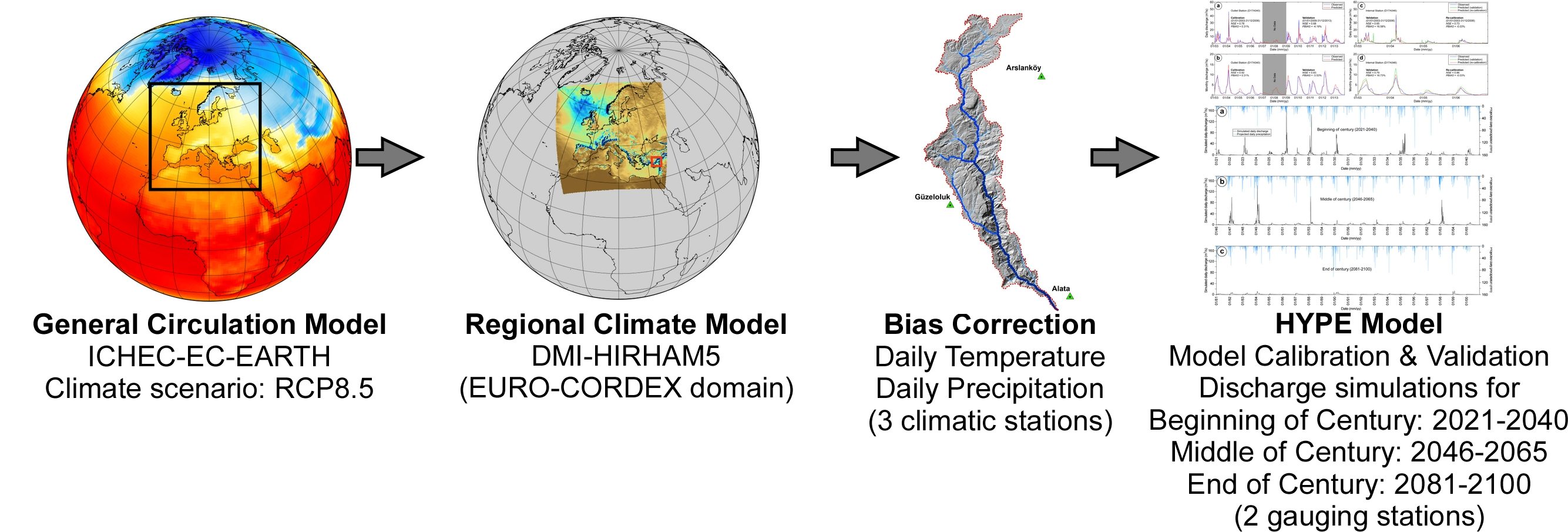
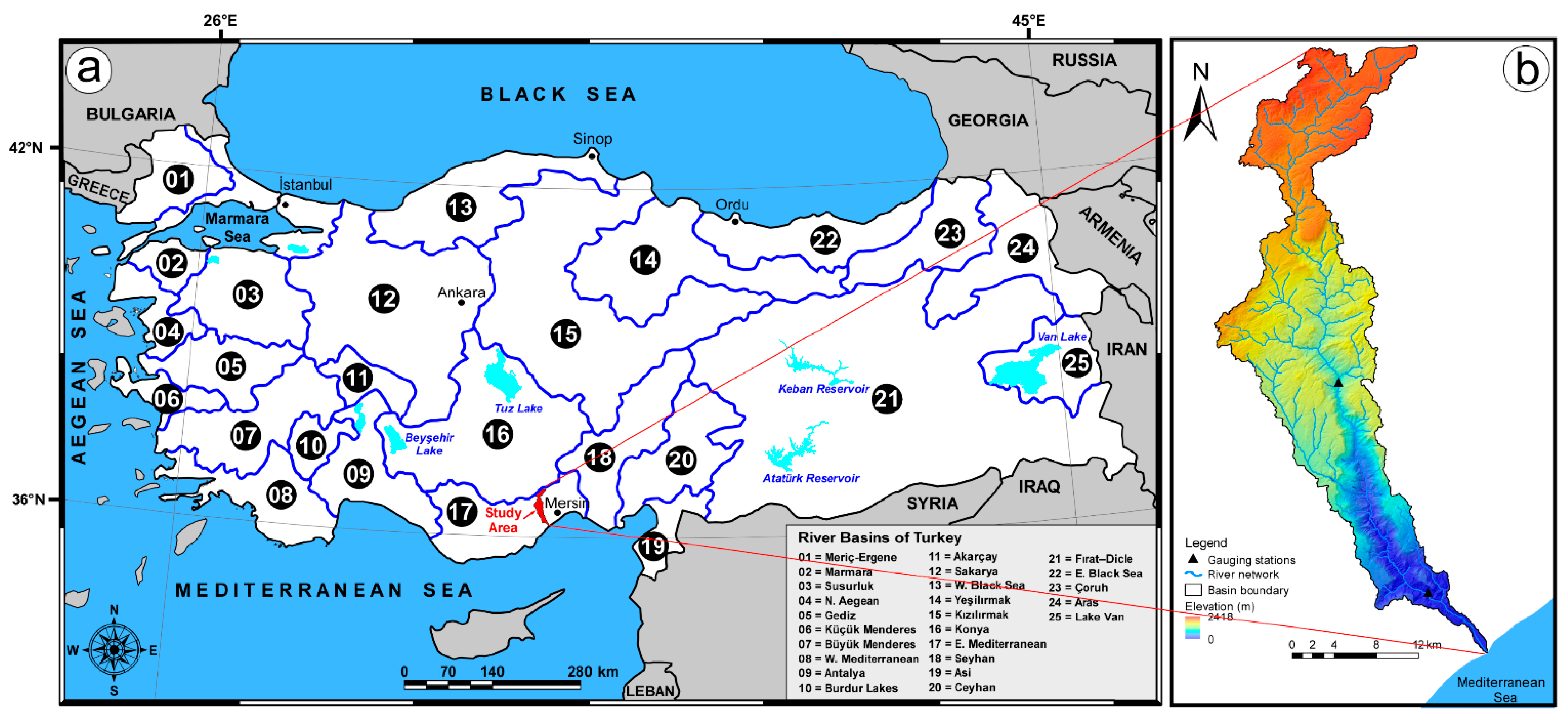
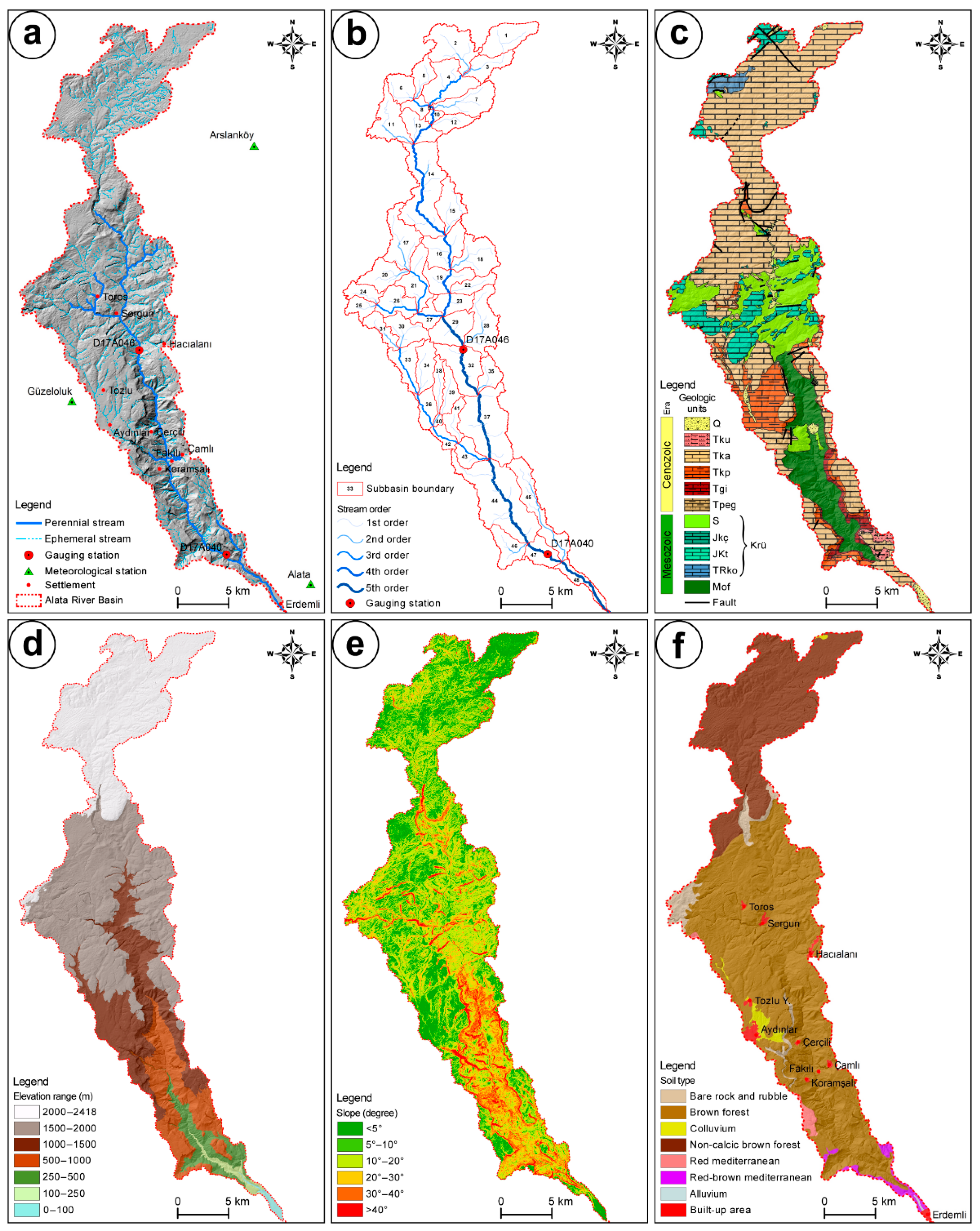
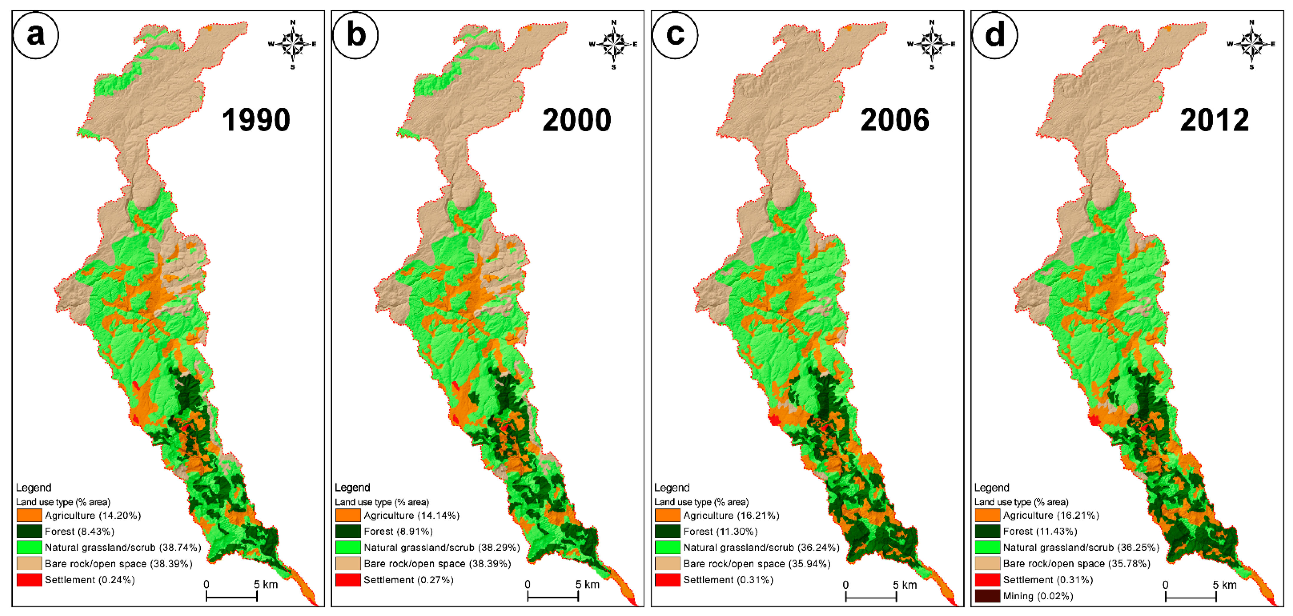
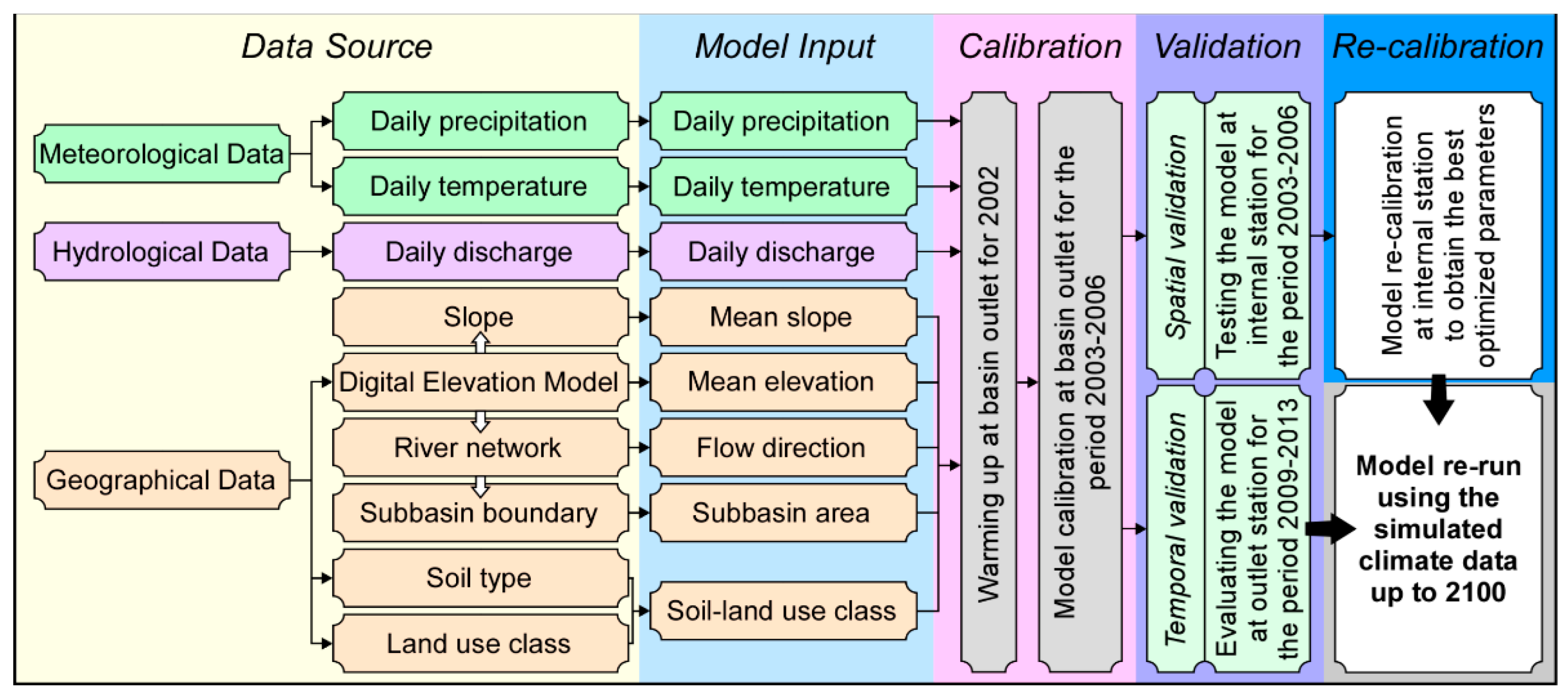
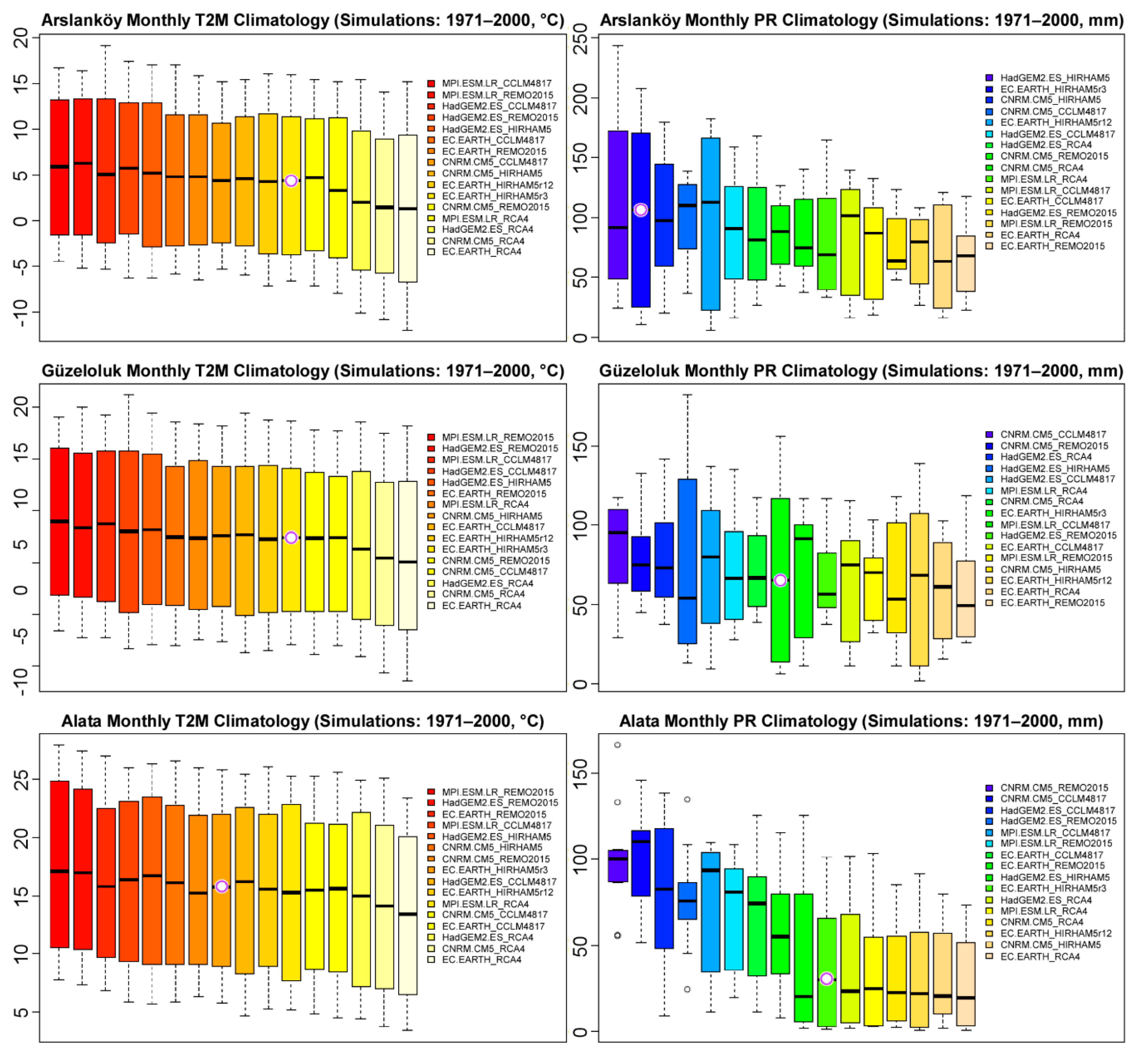
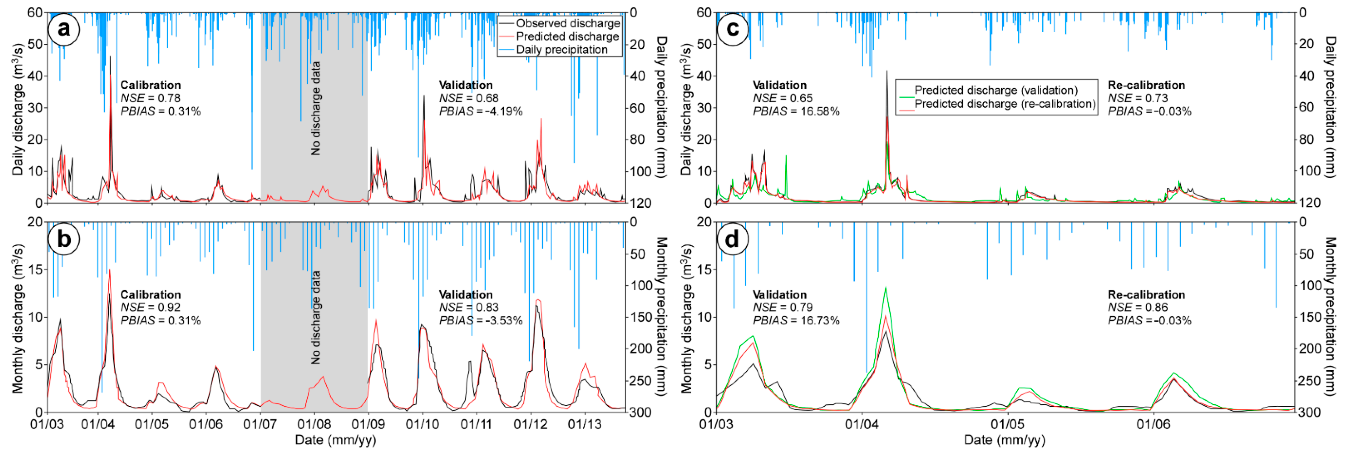
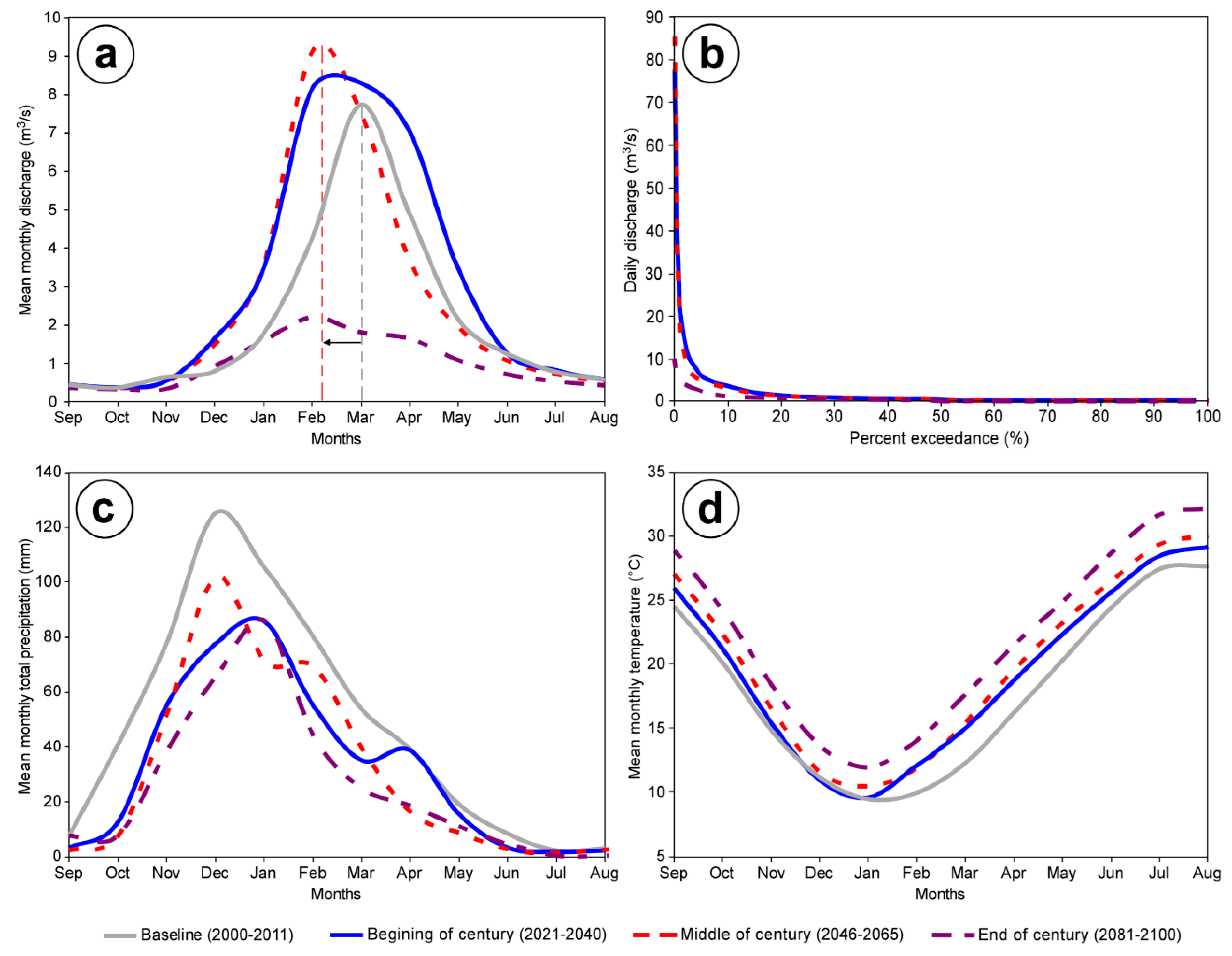
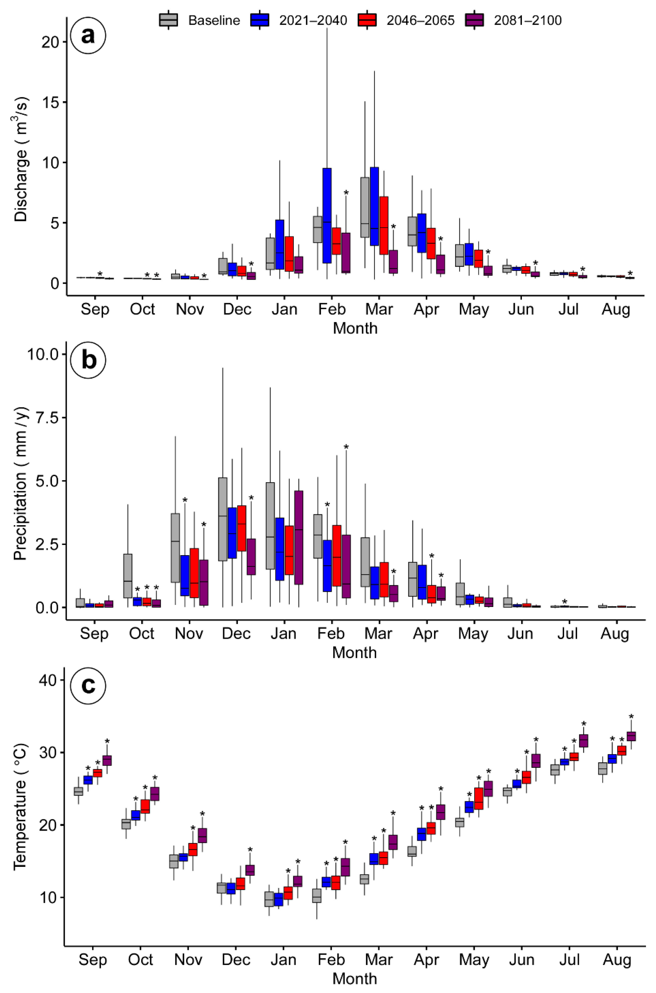
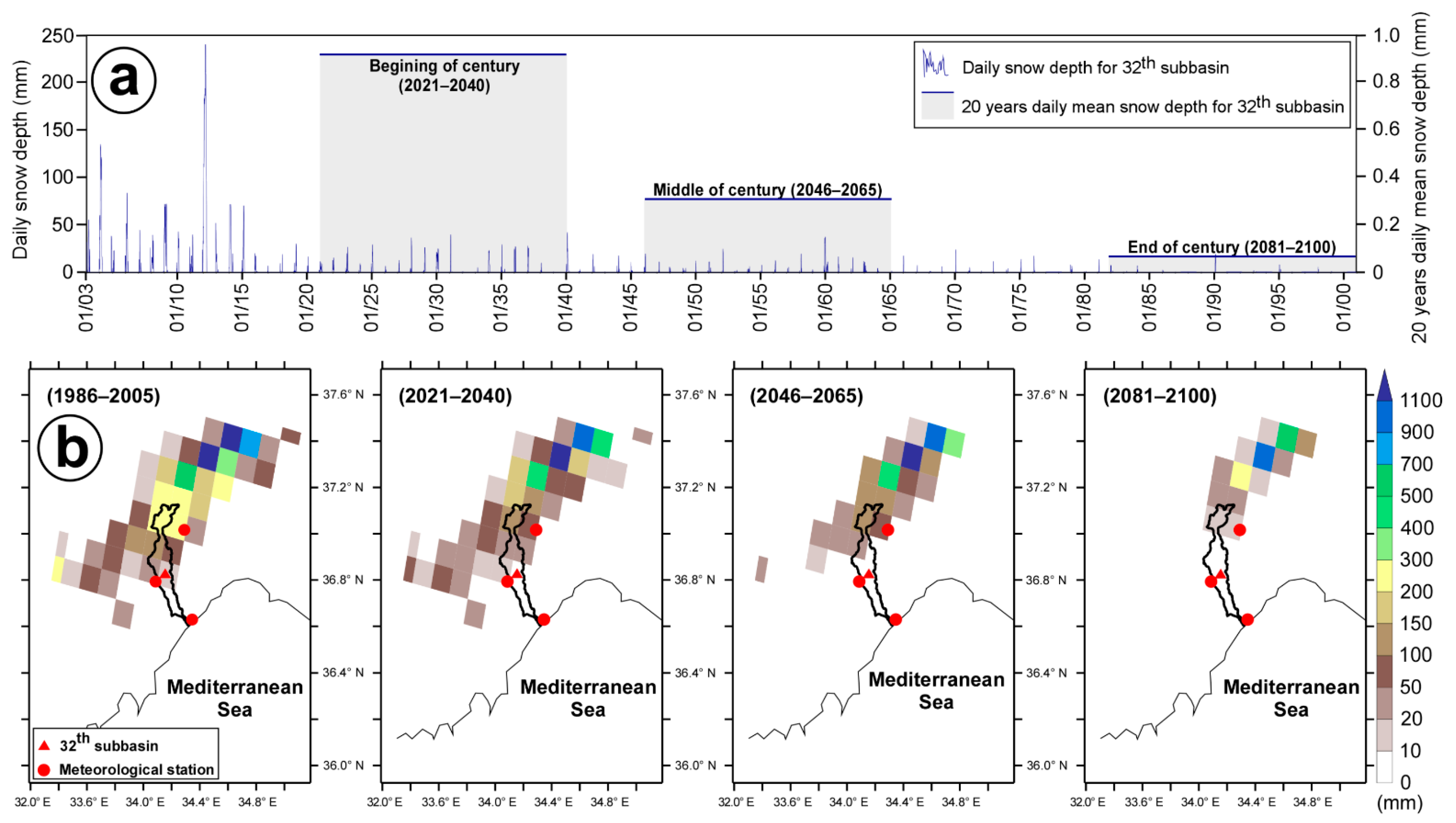
Table 1.
Basic characteristics of the Alata River Basin (ARB) in Mersin, SE Turkey.
| Characteristics | Unit | Value | Characteristics | Unit | Value |
|---|---|---|---|---|---|
| Basin area (total) | km2 | 449.19 | Elevation range | ||
| Total stream length | km | 811.57 | 0–100 m | % area | 0.59 |
| Drainage density | km/km2 | 1.80 | 100–250 m | % area | 1.14 |
| Strahler’s stream order | – | 5 | 250–500 m | % area | 4.41 |
| Hydrology (2000–2013) | 500–1000 m | % area | 11.01 | ||
| Discharge at outlet (daily mean) | m3/s | 2.99 | 1000–1500 m | % area | 17.57 |
| Precipitation (total mean) a | mm/y | 610.7 | 1500–2000 m | % area | 37.06 |
| Temperature (mean) a | °C | 12.1 | 2000–2418 m | % area | 28.22 |
| Lithology | Slope range | ||||
| Unconsolidated sediments | % area | 1.74 | 0–5° | % area | 19.28 |
| Sedimentary rocks | % area | 11.28 | 5–10° | % area | 23.01 |
| Carbonate rocks | % area | 62.61 | 10–20° | % area | 33.48 |
| Ophiolitic rocks | % area | 24.37 | 20–30° | % area | 8.03 |
| Soil type | 30–40° | % area | 12.67 | ||
| Bare rock and rubble | % area | 4.08 | >40° | % area | 3.53 |
| Brown forest | % area | 62.37 | Land use (in 2012) | ||
| Colluvium | % area | 1.32 | Agriculture | % area | 16.21 |
| Non-calcic brown forest | % area | 28.86 | Forest | % area | 11.43 |
| Red mediterranean | % area | 0.76 | Natural grassland/scrub | % area | 36.25 |
| Red-brown mediterranean | % area | 1.54 | Bare rock/open space | % area | 35.78 |
| Alluvium | % area | 0.05 | Settlement | % area | 0.31 |
| Built-up area | % area | 1.02 | Mining | % area | 0.02 |
Note: The data sources used to derive the basic characteristics of the ARB are presented in Table 2. a Thiessen polygon method was used to spatially extrapolate and calculate precipitation and temperature.
Table 2.
Time-series and spatial data used to setup and evaluate the HYPE model in the Alata River Basin (ARB). The periods 2003–2006 and 2009–2013 were used for model calibration and validation, respectively.
Table 2.
Time-series and spatial data used to setup and evaluate the HYPE model in the Alata River Basin (ARB). The periods 2003–2006 and 2009–2013 were used for model calibration and validation, respectively.
| Data Type | Data Description | Resolution | Period/Date | Source |
|---|---|---|---|---|
| Meteorological | Air temperature (°C) (3 climate stations) | Daily | 2002–2013 | Turkish State Meteorological Service [52] |
| Precipitation (mm) (3 climate stations) | Daily | 2002–2013 | Turkish State Meteorological Service [52] | |
| Hydrological | Discharge (m3/s) (2 gauging stations) | Daily | 2000–2013 (outlet) 2002–2013 (internal) | General Directorate of State Hydraulic Works [51] |
| Geographical | Digital Elevation Model (DEM) | 15 m | 1989 and 1990 | General Directorate of Mapping: Karaman N32 (d2–d4) and Silifke O32 (a1–a4, c1, c4, d2) 1:25,000-scale topographic maps with 10-m contour interval |
| Geology | 1:25,000 | 1998 and 2007 | [53,54] | |
| Soil type | 1:25,000 | 2001 | General Directorate of Rural Services [55] | |
| Land use | 100 m | 2012 | CORINE Land Cover 2012 (Release 18.5) [58,59] |
Table 3.
The HYPE model’s best-optimised parameters for the Alata River Basin (ARB) outlet and internal gauging stations.
Table 3.
The HYPE model’s best-optimised parameters for the Alata River Basin (ARB) outlet and internal gauging stations.
| Parameter a | Physical Meaning and Unit | Dependence | Optimised Value | |
|---|---|---|---|---|
| Outlet | Internal | |||
| ttmp | Threshold temperature for snowmelt and evaporation (°C) | Land use | ||
| Agriculture | 0.770 | 0.880 | ||
| Natural grassland/scrub | 0.219 | 0.159 | ||
| cevp | Potential evaporation rate (mm/d/°C) | Land use | ||
| Agriculture | 0.828 | 0.918 | ||
| Natural grassland/scrub | 0.999 | 1.229 | ||
| cevpph | Phase of the sinus function that corrects potential evaporation (d) | General | 179.5 | 158.5 |
| srrate | Rate of surface runoff (–) | Soil type | ||
| Brown forest soil | 0.0067 | 0.0047 | ||
| Non-calcic brown forest soil | 0.0098 | 0.0058 | ||
| cmlt | Melting parameter for snow (mm/d/°C) | Land use | ||
| Agriculture | 2.013 | 2.173 | ||
| Natural grassland/scrub | 1.902 | 1.785 | ||
| rrcs2 | Recession coefficient for the lowermost soil layer (–) | Soil type | ||
| Colluvial soil | 0.00958 | 0.00158 | ||
| Brown forest soil | 0.00602 | 0.00402 | ||
| damp | Fraction of delay time in river through damping (–) | General | 0.683 | 0.983 |
| macro1 | Rate of the macropore flow (macrate) (–) | Soil type | ||
| Brown forest soil | 7.518 | 9.519 | ||
| Non-calcic brown forest soil | 5.545 | 7.543 | ||
| macro2 | Threshold for the macropore flow (mactresin) (mm) | Soil type | ||
| Brown forest soil | 4.814 | 4.914 | ||
| Non-calcic brown forest soil | 0.815 | 6.059 | ||
| macro3 | Threshold of the soil moisture for macropore flow and surface runoff (mactressm) (–) | Soil type | ||
| Brown forest soil | 0.461 | 0.361 | ||
| Non-calcic brown forest soil | 0.815 | 0.855 | ||
| wcfc | Field capacity as a fraction, same for all soil layers (–) | Soil type | ||
| Non-calcic brown forest soil | 0.959 | 0.859 | ||
| wcwp | Wilting point as a fraction (–) | Soil type | ||
| Brown forest soil | 0.011 | 0.031 | ||
| wcep | Effective porosity as a fraction, same for all soil layers | Soil type | ||
| Brown forest soil | 0.000375 | 0.000225 | ||
a Further details on the HYPE model parameters and other variables can be found in Lindström et al. [35].
Table 4.
Summary of the significance levels (p-values) of the Wilcoxon rank-sum test for the discharge, precipitation and temperature during the three projection periods (beginning of the century, middle of the century and end of the century) compared to the reference period (baseline). Significant p-values (≤0.05) are in bold.
| Discharge | Precipitation | Temperature | |||||||
|---|---|---|---|---|---|---|---|---|---|
| Months | Beginning 2021–2040 | Middle 2046–2065 | End 2081–2100 | Beginning 2021–2040 | Middle 2046–2065 | End 2081–2100 | Beginning 2021–2040 | Middle 2046–2065 | End 2081–2100 |
| September | 0.88 | 0.15 | <0.05 | 0.65 | 0.81 | 0.47 | <0.05 | <0.05 | <0.05 |
| October | 0.98 | <0.05 | <0.05 | <0.05 | <0.05 | <0.05 | <0.05 | <0.05 | <0.05 |
| November | 0.32 | 0.06 | <0.05 | <0.05 | 0.06 | <0.05 | 0.06 | <0.05 | <0.05 |
| December | 1.00 | 0.55 | <0.05 | 0.46 | 0.55 | <0.05 | 0.48 | 0.18 | <0.05 |
| January | 0.64 | 0.91 | 0.09 | 0.30 | 0.18 | 0.41 | 0.72 | <0.05 | <0.05 |
| February | 0.82 | 0.24 | <0.05 | <0.05 | 0.12 | <0.05 | <0.05 | <0.05 | <0.05 |
| March | 0.58 | 0.45 | <0.05 | 0.06 | 0.13 | <0.05 | <0.05 | <0.05 | <0.05 |
| April | 0.91 | 0.27 | <0.05 | 0.83 | <0.05 | <0.05 | <0.05 | <0.05 | <0.05 |
| May | 1.00 | 0.31 | <0.05 | 0.62 | 0.13 | 0.06 | <0.05 | <0.05 | <0.05 |
| June | 0.98 | 0.29 | <0.05 | 0.30 | 0.20 | 0.10 | <0.05 | <0.05 | <0.05 |
| July | 0.98 | 0.31 | <0.05 | <0.05 | 0.13 | 0.15 | <0.05 | <0.05 | <0.05 |
| August | 0.85 | 0.29 | <0.05 | 0.22 | 0.09 | 0.31 | <0.05 | <0.05 | <0.05 |
Publisher’s Note: MDPI stays neutral with regard to jurisdictional claims in published maps and institutional affiliations. |
© 2021 by the authors. Licensee MDPI, Basel, Switzerland. This article is an open access article distributed under the terms and conditions of the Creative Commons Attribution (CC BY) license (http://creativecommons.org/licenses/by/4.0/).
Share and Cite
MDPI and ACS Style
Yıldırım, Ü.; Güler, C.; Önol, B.; Rode, M.; Jomaa, S. Modelling of the Discharge Response to Climate Change under RCP8.5 Scenario in the Alata River Basin (Mersin, SE Turkey). Water 2021, 13, 483. https://doi.org/10.3390/w13040483
AMA Style
Yıldırım Ü, Güler C, Önol B, Rode M, Jomaa S. Modelling of the Discharge Response to Climate Change under RCP8.5 Scenario in the Alata River Basin (Mersin, SE Turkey). Water. 2021; 13(4):483. https://doi.org/10.3390/w13040483
Chicago/Turabian StyleYıldırım, Ümit, Cüneyt Güler, Barış Önol, Michael Rode, and Seifeddine Jomaa. 2021. "Modelling of the Discharge Response to Climate Change under RCP8.5 Scenario in the Alata River Basin (Mersin, SE Turkey)" Water 13, no. 4: 483. https://doi.org/10.3390/w13040483
Note that from the first issue of 2016, this journal uses article numbers instead of page numbers. See further details here.