Integrating the JRC Monthly Water History Dataset and Geostatistical Analysis Approach to Quantify Surface Hydrological Connectivity Dynamics in an Ungauged Multi-Lake System

Abstract

Determining the dynamics of surface hydrological connectivity in a landscape of multiple lakes with different sizes and depths is challenging. This is especially the case for ungagged, large areas of multi-lake systems. Integrated use of remote sensing and geostatistical analysis can be a useful approach for developing metrics that can be used to identify the hydrological connectivity and their changes. In this study, we conducted a geostatistical analysis of 18 wet and dry binary state rasters derived from Landsat images over a large ungauged multi-lake system, the Momoge National Nature Reserve in Northeast China. Our goal was to investigate applicability and dynamics of three surface hydrological connectivity metrics, namely, geostatistical connectivity function (GCF), maximum distance of connection (MDC), and surface water extent (SWE) of the top 10 largest connectomes (i.e., seasonally connected water bodies). We found that, during a dry year, the reduction rate of the GCF curve was slower along the west–east (W–E) direction than along the north–south (N–S) direction, which was contrary to the patterns exhibited in a normal or wet year. The minimum values of the MDC in W–E and N–S directions in the dry year were 22.4 km and 6.3 km, respectively, while the maximum values of the MDC along the above two directions in the wet year were 50.7 km and 65.1 km, respectively. The components and spatial distribution of the top 10 largest connectomes changed dramatically in different months of each hydrological year, resulting in a huge change in the monthly SWE of the top 10 largest connectomes. Overall, this study validated the usefulness of combining remote sensing image analysis with geostatistical methods to quantify the surface hydrological connectivity from different perspectives in an ungauged area. The approach may be applicable to studies in other geographical regions, to guide water resources and wetland management practices.

1. Introduction

Globally, approximately 90,000 km² of surface water area disappeared and 184,000 km² area of water surfaces formed between 1984 and 2015 [1]. The changes have been attributed to both climate change and human activities, such as natural drying, river diversion, reservoir filling, damming, and unregulated withdrawal [2,3,4,5]. Changes in water surface area can affect surface hydrological connectivity and, in turn, the transport of water-mediated matter, energy, and organisms within or between hydrological cycle elements. In order to maintain the ecological integrity and functions of surface water systems, it is necessary to conduct cost-effective and efficient monitoring and evaluation of the hydrological connectivity of these systems. However, due to the lack of appropriate methods and indicators, it is still a challenge to quantitatively assess the hydrological connectivity of a landscape composed of multiple lakes of different sizes and depths.

Satellite remote sensing has been used as a tool for the acquisition of timely and repetitive information on surface water bodies at large scales, which provides data for assessing surface hydrological connectivity. For instance, optical images from Landsat and Moderate Resolution Imaging Spectrometer (MODIS) or their fusions have been successfully used to quantify the hydrological connectivity among rivers, floodplains, and lakes [6,7,8,9]. In recent years, some big data exploration and information extraction techniques (i.e., the “expert systems” [10,11], “visual analytics” [1], and “evidential reasoning” [12]) were developed to accurately extract global surface water bodies from Landsat images. The resulting free-access dataset (i.e., the monthly water history dataset from the Joint Research Centre of the European Commission, hereinafter referred to as the JRC Monthly Water History dataset) is available in Google Earth Engine. However, few attempts have been made to use this dataset to quantify surface hydrological connectivity.

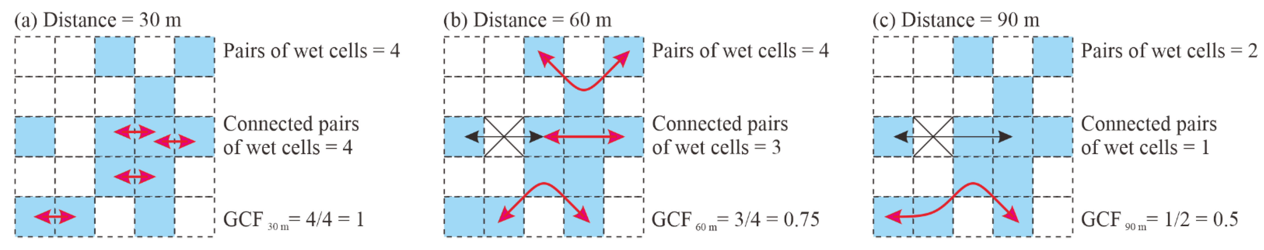
In addition to data, surface hydrological connectivity assessment must be supported by an indicator or a set of indicators [13]. These indicators can be timing, frequency, surface water extent, flow path, etc. [14]. In the recent decade, a set of new indicators was developed through assessing remote sensing data with geostatistical methods. These include the geostatistical connectivity function (GCF) [6] and maximum distance of connection (MDC). Several studies [6,7,8,9] have applied the GCF and MDC to quantify surface hydrological connectivity among rivers, floodplains, and lakes under the influence of flood pulses. However, there is a significant knowledge gap regarding the combined impact of artificial replenishment water and flooding on GCF and MDC.

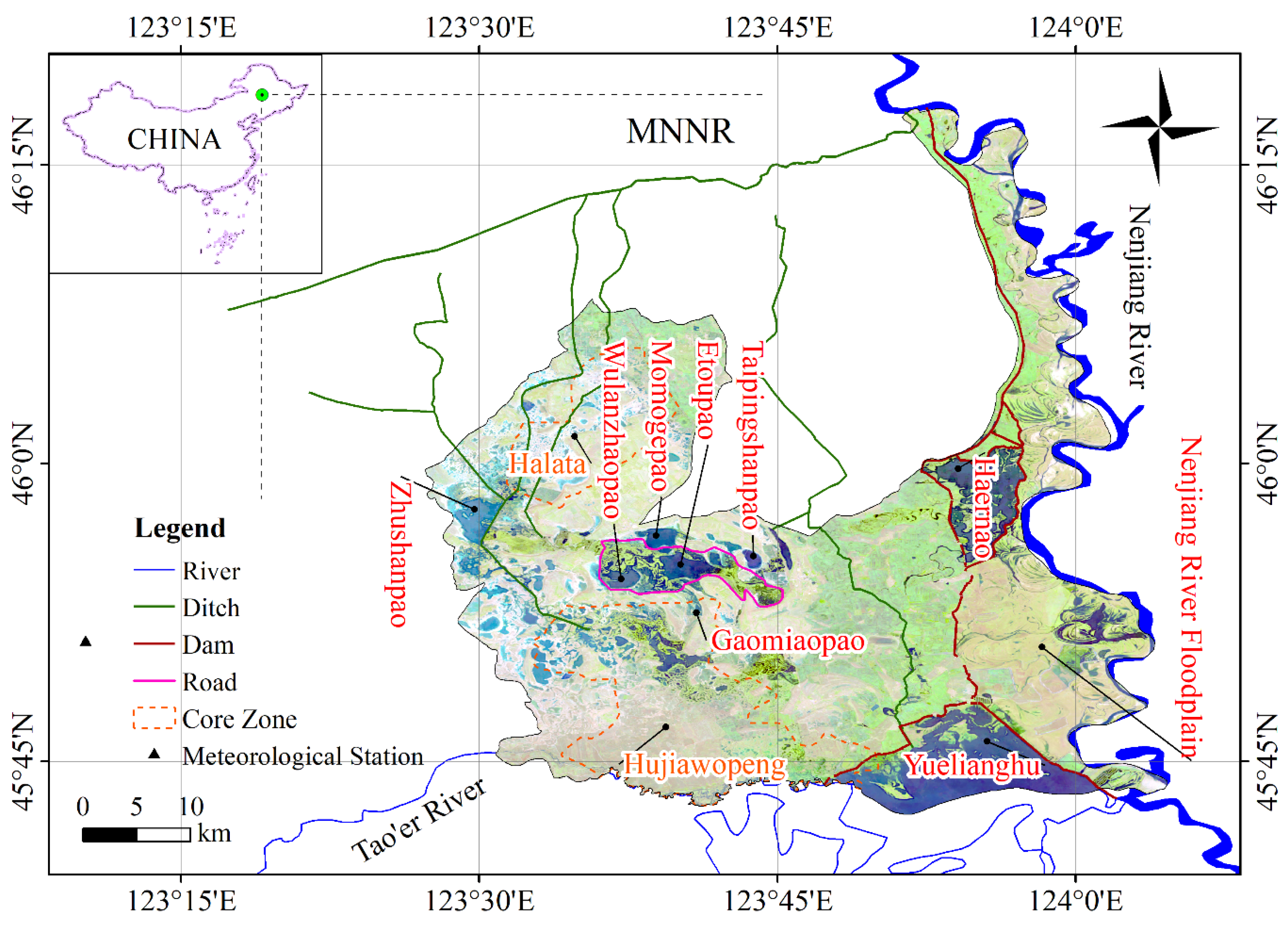
To address this knowledge gap, we combined the JRC Monthly Water History data and geostatistical approach to analyze the dynamics of surface hydrological connectivity of a multi-lake system during a dry, a normal, and a wet year. We took China’s Momoge National Nature Reserve (a Ramsar site) as a case study because it broadly represents the widespread landscape with relatively shallow lakes fed by rivers and manmade canals. Specifically, this study aimed to (1) analyze changing trends in the geostatistical connectivity function and maximum distance of connection along the west–east (W–E) and north–south (N–S) directions during different hydrological years, (2) identify the spatiotemporal distribution and connection process of seasonal connected water bodies during different hydrological years, and (3) quantify the variation in surface water extent of the top 10 largest connectomes during different hydrological years. In our previous paper [15], we used Sentinel-1 synthetic aperture radar (SAR) data and a geostatistical analysis approach to quantitatively evaluate surface hydrological connectivity dynamics over five normal years in the same study area. Therefore, the results of the current manuscript can be regarded as a supplement to the previous paper. Since the study area undergoes a dry–wet transition every 10 years, the current manuscript is more important for water resource management in the study area.

2. Materials and Methods

2.1. Study Area

The Momoge National Nature Reserve (MNNR, 45°42′25″–46°18′00″ N, 123°27′00″–124°04′33.7″ E) is located in Zhenlai County, west Jilin Province, Northeast China, covering an area of 1440 km² (Figure 1). The reserve is one of the internationally important “Ramsar wetland sites”, as it provides habitats for the annual migrations of several rare and endangered birds, such as Siberian crane (Grus leucogeranus), red-crowned crane (Grus japonensis), and Oriental white stork (Ciconia ciconia). The terrain is flat and the altitude ranges from 128 m to 168 m. Two large rivers flow through the reserve, including a permanently inundated river (Nenjiang River) and a temporary river (Tao’er River). The reserve has many seasonally connected large lakes and reservoirs, including Zhushanpao, Wulanzhaopao, Momogepao, Etoupao, Taipingshanpao, Gaomiaopao, Haernao, and Yuelianghu (Figure 1). A large number of small lakes are located in the Halata core zone, the Hujiawopeng core zone, and the Nenjiang River floodplain in the reserve. Unlike the lakes on the Nenjiang River floodplain that are mainly supplied by floods, some lakes in the central and western parts of the MNNR are mainly recharged by artificial ditches in May, August, and September. An extensive dam in the east and a road around the Etoupao and the Wulanzhaopao obstruct the connection between water bodies (Figure 1).

The climate of the study can be characterized as temperate continental monsoon, with a monthly mean temperature ranging from −17.4 °C in January to 23.5 °C in July. The annual mean precipitation is 385.7 mm, 90% of which is concentrated during May and October, whereas the annual mean evapotranspiration is 1530.1 mm [16]. The average annual freezing period starts on 24 October and the average annual thawing period starts on 2 May [17].

2.2. Remote Sensing Data and Preprocessing

In this study, we utilized the JRC Monthly Water History dataset (JRC Monthly Water History v1.2, Source: EC JRC/Google) which is derived from three million Landsat 5, 7, and 8 images at 30 m spatial resolution. This dataset contains maps of the location and temporal distribution of global surface water from 1984 to 2019 and provides statistics on the extent and change of those water surfaces. In the dataset, each pixel was individually classified into water/non-water using an expert system, visual analytics, and evidential reasoning. The dataset consists of three bands, among which band 0 is the “no data” class, band 1 is the “not water” class, and band 2 is the “water” class. The classifier produces less than 1% false water detections and misses less than 5% of water [1]. For more details about this dataset, see the literature [1].

We first selected a total of 18 maps from May to October during 2000 (a dry year), 2013 (a wet year), and 2019 (a normal year) from the JRC dataset, and we cropped them to the study area in Google Earth Engine. Then, by reclassifying the “water” class as 1, and reclassifying the “no data” and “not water” classes as 0, a wet and dry binary state raster dataset was made for the subsequent processing. The process of reclassification was done using ArcGIS software (version 10.7, Environmental Systems Research Institute, Redlands, CA, USA).

2.3. Geostatistical Connectivity Analysis

The geostatistical connectivity function (GCF) is used to assess the surface hydrological connectivity dynamics. The GCF expresses the probability that n pixels along a given direction are all higher than the threshold $z_c$ [18].

$$P(n;z_c)=\mathrm{Pr}\left\{{\displaystyle \prod _{j=1}^{n}I(u_j;z_c)=1}\right\}$$

(1)

where $I(u_j;z_c)$ is an indicator of $z(u_j)$ at location $u_j$ that is higher than the threshold $z_c$. If $z(u_j)>z_c$, then $I(u_j;z_c)=1$; else, if $z(u_j)<z_c$, then $I(u_j;z_c)=0$. It is estimated when the starting wet pixel $u_1$ is located at all possible positions. As a result, the value of GCF at any given distance is the ratio of connected wet pixel pairs along a given direction to all (that is, isolated and connected) wet pixel pairs.

The geostatistical connectivity analysis was performed with a Matlab script provided by Trigg et al. [6]. The script analyzes the wet and dry binary state raster and calculates GCF along four directions, namely west–east (W–E), north–south (N–S), northwest–southeast (NW–SE), and northeast–southwest (NE–SW), assuming eight-way connectivity. This study only analyzed the surface hydrological connectivity between water bodies along the W–E and N–S directions, because surface waters in the study area are connected mainly along these two directions. Specifically, the surface hydrological connectivity directions between the Tao’er River and the study area and between the Nenjiang River and the study area are mainly west–east, while the surface hydrological connectivity directions between artificial ditches and the study area are mainly north–south. A simple example shows how to calculate the GCF along the W–E direction [15] (Figure 2). In addition, the script also creates a grid, where each of the connected objects (i.e., connectome) is identified by an integer from 1 to n. On this basis, we determined and mapped the top 10 largest connectomes in each month. Afterward, the surface water extent of the top 10 largest connectomes was also calculated. These processes were done in the Matlab software (version R2014a, The MathWorks, Inc., Natick, MA, USA) and the Arcgis software.

2.4. Meteorological Data

Meteorological data for the study area were collected from the China Meteorological Data Service Center (http://data.cma.cn). These meteorological data include monthly mean precipitation and evaporation at a meteorological station from May to October in 2000, 2013, and 2019. The location of the meteorological station is shown in Figure 1. These meteorological data were used to determine the relationship between these meteorological elements and the SWE of the top 10 largest connectomes. The process was done in the Origin software (version 2020b, Origin Lab Corporation, Northampton, MA, USA).

3. Results

3.1. Variations in the GCF

Using the wet and dry binary state rasters derived from the JRC Monthly Water History dataset, the application of the geostatistical connectivity analysis generated a series of connectivity curves that describe the surface hydrological connectivity dynamics of a multi-lake system fed by rivers and artificial channels. For comparison, the geostatistical connectivity function (GCF) curves along the west–east and north–south directions for a dry year (from May to October 2000), a normal year (from May to October 2019), and a wet year (from May to October 2013) are illustrated in Figure 3.

In a dry year (Figure 3a), the reduction rate of the GCF curve along the W–E direction increased from May to August, remained almost unchanged from August to September, and then decreased from September to October, indicating that the GCF was better in August and September and worse in the other months. The maximum distance of connection (MDC, i.e., the distance at which the GCF curve reaches zero) in each month was very close, ranging from 22.4 km to 23.6 km. In a normal year (Figure 3b), the reduction rate of the GCF curve along the W–E direction gradually slowed down with the passage of a month, indicating that the GCF improved from May to October. The MDC varied each month, ranging from 23.6 km to 36.4 km. In a wet year (Figure 3c), the reduction rate of the GCF curve along the W–E direction decreased from May to June, increased from June to August, and decreased from August to October, showing that the GCF in August was the best. The MDC varied greatly from month to month, ranging from 23.6 km to 50.7 km.

During the dry year (Figure 3d), the reduction rate of the GCF curve along the N–S direction showed little difference from month to month. The MDC varied each month, ranging from 6.3 km to 12.2 km. During the normal year (Figure 3e), the reduction rate of the GCF curve along the N–S direction increased from May to September and decreased from September to October, indicating that the GCF in September was the best. The MDC changed a lot every month, ranging from 10.0 km to 61.7 km. During the wet year (Figure 3f), the reduction rate of the GCF curve along the N–S direction increased from May to August and then decreased from August to October, showing that the GCF in August was the best. The MDC varied greatly every month, ranging from 12.5 km to 65.1 km.

3.2. Spatiotemporal Distribution and Connection Process of Connectomes

The input and the flow of water created a number of seasonally connected water bodies in the study area. In order to further study the flow path and connection process of connectomes, Figure 4, Figure 5 and Figure 6 depict the monthly distribution of the top 10 largest connectomes of the study area in dry, normal, and wet years.

In the dry year (Figure 4), Etoupao was first connected to Wulanzhaopao and Gaomiaopao through channels in May and disconnected from these two lakes between June and October. Similarly, in May, Haernao was first connected to the Nenjiang river through a floodplain channel and separated from it between June and October. In contrast, Yuelianghu was first connected to the Nenjiang River through an artificial channel in May and then disconnected and reconnected to it in June and September, respectively. In addition, except for September, within the six months, some lakes in the Hujiawopeng core zone were connected to each other through “fill and merge”.

In the normal year (Figure 5), Etoupao was first connected to Wulanzhaopao through a channel in May and then disconnected and reconnected to it in July and September, respectively. In contrast, Etoupao was first connected to Gaomiaopao by over-road flow in May and then disconnected and reconnected to it in June and September, respectively. Haernao was connected to the Nenjiang River floodplain via overbank flow from August to October. Yuelianghu was first connected to the Nenjiang River through an artificial channel in May and then disconnected and reconnected to it in July and August, respectively. Furthermore, Yuelianghu was connected to the Nenjiang River floodplain via the artificial channel from August to October. It is worth noting that Haernao, Nenjiang River floodplain, and Yuelianghu were flooded and joined together from September to October. In June, some lakes in the Halata core zone were connected to each other through “fill and merge”. In contrast, except for June, within the six months, some lakes in the Hujiawopeng core zone were connected to each other through “fill and merge”.

In the wet year (Figure 6), during the six months from May to October, Etoupao was connected to Wulanzhaopao through channels, whereas it was connected to Momogepao and Gaomiaopao via over-road flow. In contrast, Etoupao was first connected to Taipingshanpao through over-road flow in May and then disconnected from it in June and reconnected to it in August. Haernao was first connected to the Nenjiang River in May through the floodplain channel and disconnected from it between June and July. During the six months, Yuelianghu was always connected to the Nenjiang River through an artificial channel. In July, Yuelianghu was first connected to the Nenjiang River floodplain through the artificial channel. From August to October, Haernao, Nenjiang River floodplain, and Yuelianghu were flooded and joined together; meanwhile, some lakes in the Halata core zone were connected to each other via “fill and merge”. In September and October, Zhushanpao was connected to the lakes in Halata core zone. Furthermore, lots of lakes in the Hujiawopeng core zone were connected to each other via “fill and merge” throughout the six months.

3.3. Changes in SWE of the Top 10 Largest Connectomes

During the dry year, the surface water extent of the top 10 largest connectomes first decreased rapidly from May to June, then decreased slowly from June to September, and finally increased slowly from September to October (

Table 1. Changes in surface water extent (SWE, km²) of the top 10 largest connectomes in the Momoge National Nature Reserve, China during dry, normal, and wet years.

	May	June	July	August	September	October
Dry year	207.11	117.35	109.08	98.06	97.75	117.32
Normal year	261.47	214.67	165.23	509.21	607.51	514.22
Wet year	347.53	335.14	556.38	812.73	859.38	858.72

). During the normal year, the SWE first declined slowly from May to July, then rose rapidly from July to September, and finally declined slowly from September to October. During the wet year, the SWE first dropped slowly from May to June, then rose rapidly from June to September, and finally dropped slowly from September to October. The changing trend of SWE reflects that the changing trend of surface hydrological connectivity in different hydrological years was quite different.

4. Discussion

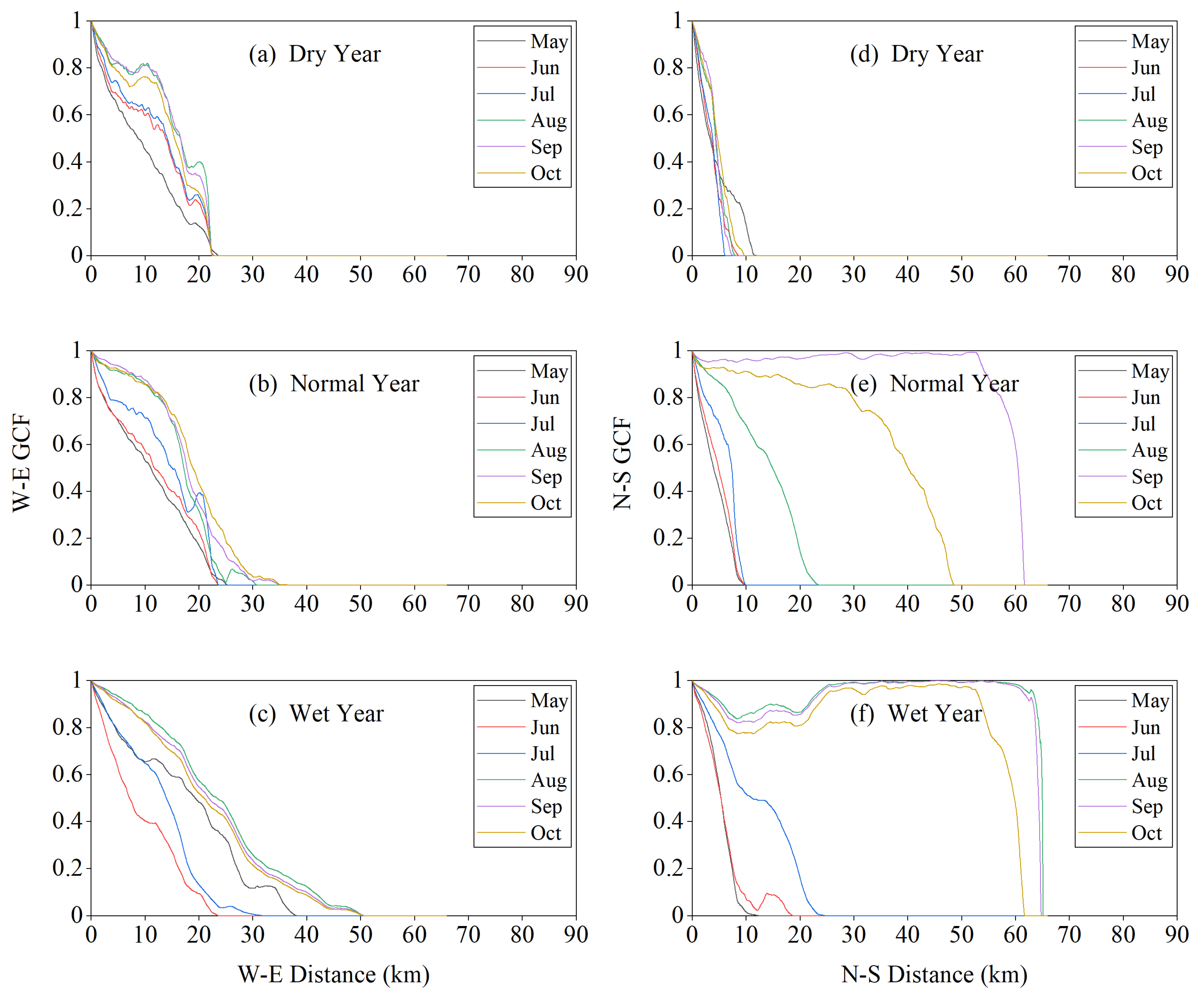
Our results show that, during the dry year, the reduction rate of the GCF curve was slower along the W–E direction than that along the N–S direction, which is contrary to the situation during the normal and wet years (Figure 3). As far as normal years are concerned, the current results of the reduction rate of the GCF curve using the JRC Monthly Water History dataset are consistent with the findings of our previous paper [15] using the Sentinel-1 dataset. Moreover, the minimum values of the MDC along the W–E and N–S directions both appeared in the dry year, at 22.4 km and 6.3 km, respectively, while the maximum values of the MDC along the above two directions both appeared in the wet year, at 50.7 km and 65.1 km, respectively (Figure 3). During the normal year, the MDC along the W–E direction varied from 23.6 km to 36.4 km, while the MDC along the N–S direction varied from 10.0 km to 61.7 km (Figure 3). Whether in the W–E direction or in the N–S direction, the changes in the MDC in the current study were more dramatic than the findings of our previous paper [15]. The reason may be that the current paper only focused on one normal year, whereas the results of our previous paper were the average of five normal years. These results indicate that, due to the combined effects of natural and human factors, such as flooding, manmade water replenishment, dams, and roads, the surface hydrological connectivity along the W–E and N–S directions in a large multi-lake system exhibited different responses. Trigg et al. [6] and Liu et al. [8] found that the surface hydrological connectivity in a river–lake system is affected by natural factors such as floods and main lake stages. Our new discovery of the difference in surface hydrological connectivity along the W–E and N–S directions in a large multi-lake system during different hydrological years expands our understanding of surface hydrological connectivity under both natural and manmade influences.

At the beginning of the 21st century, due to years of drought and upstream reservoir filling, Zhushanpao, the lakes in the Halata core zone, and the Hujiawopeng core zone have almost disappeared, whereas the remaining lake area has shrunk dramatically (Figure 4). Since then, most of the Hujiawopeng core zone has gradually been reclaimed as dry farmland. This land-use change has weakened the surface hydrological connectivity between the lakes inside and outside the Hujiawopeng core zone. In recent years, with the construction and operation of replenishment ditches, the water surface area of Zhushanpao and the lakes in the central part (i.e., Wulanzhaopao, Momogepao, Etoupao, Taipingshanpao, etc.) has increased greatly (Figure 5). However, due to excessive water, Scirpus nipponicus and Scirpus planiculmis in the Wulanzhaopao and Etoupao were submerged, preventing the Siberian cranes from obtaining food in these areas. The current results are consistent with the findings of our earlier study [15]. In addition, even in the wet year, the surface hydrological connectivity between the Nenjiang River and its floodplain in May was very poor, which may adversely affect the germination and growth of aquatic vegetation in the area.

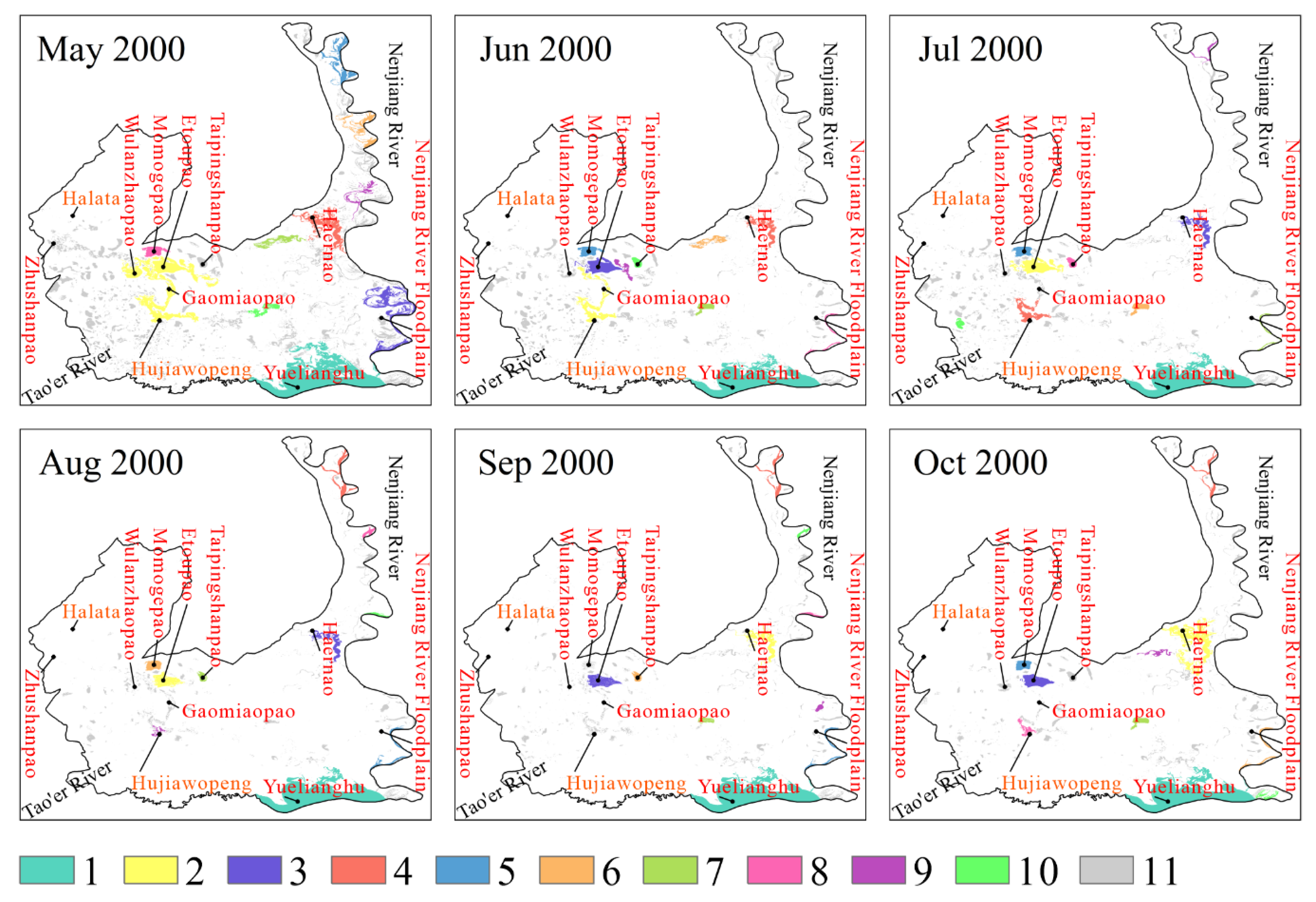
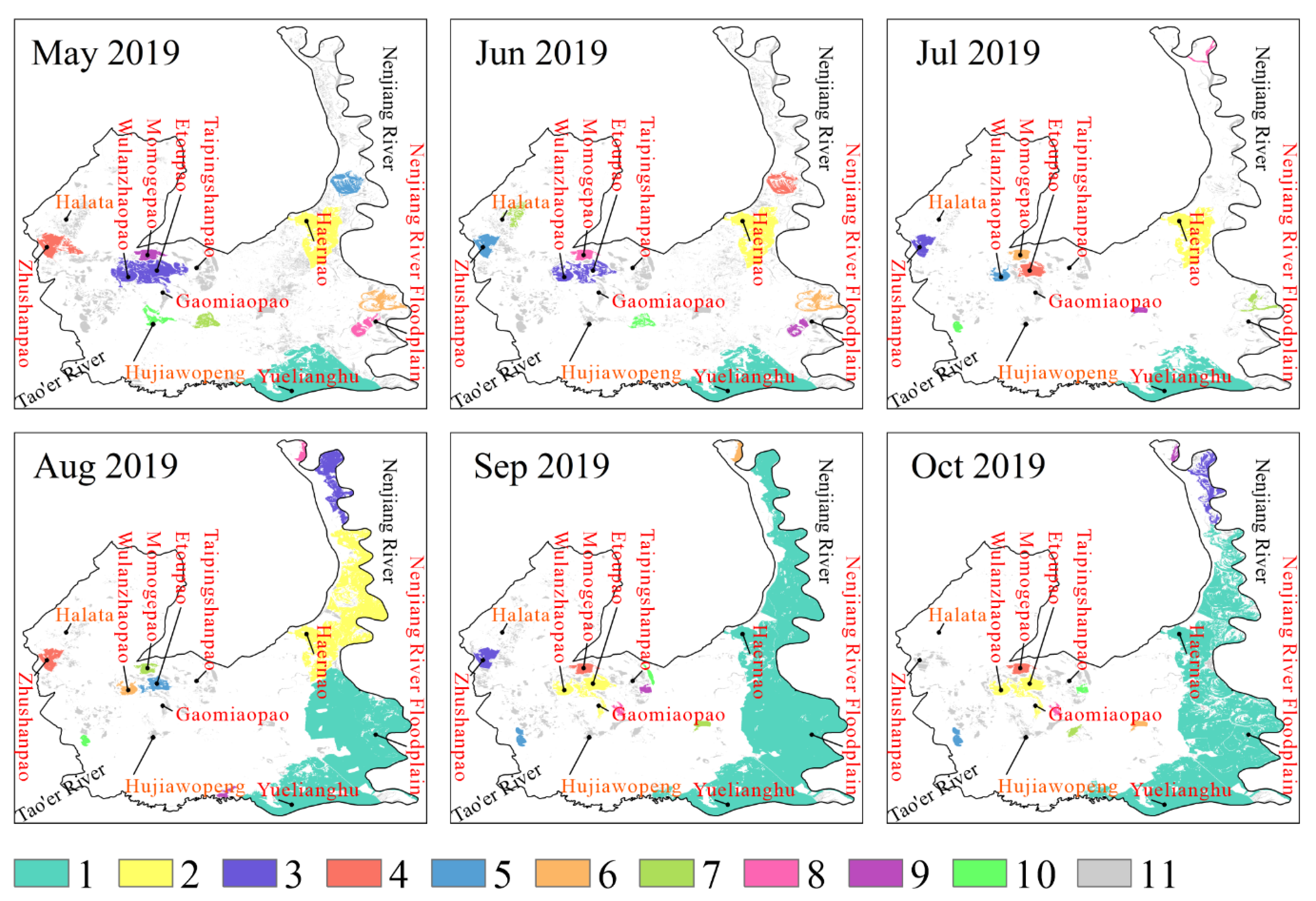
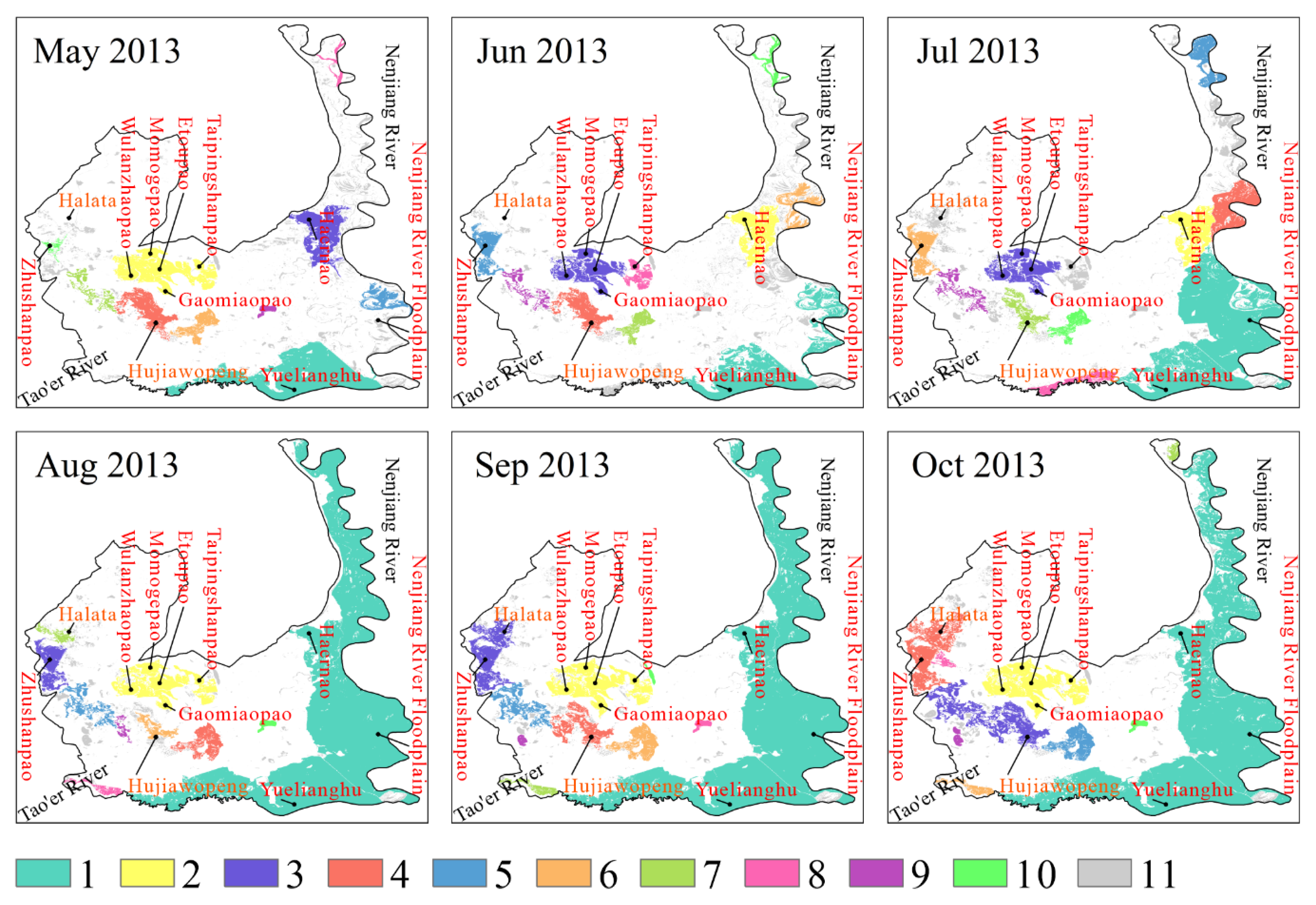
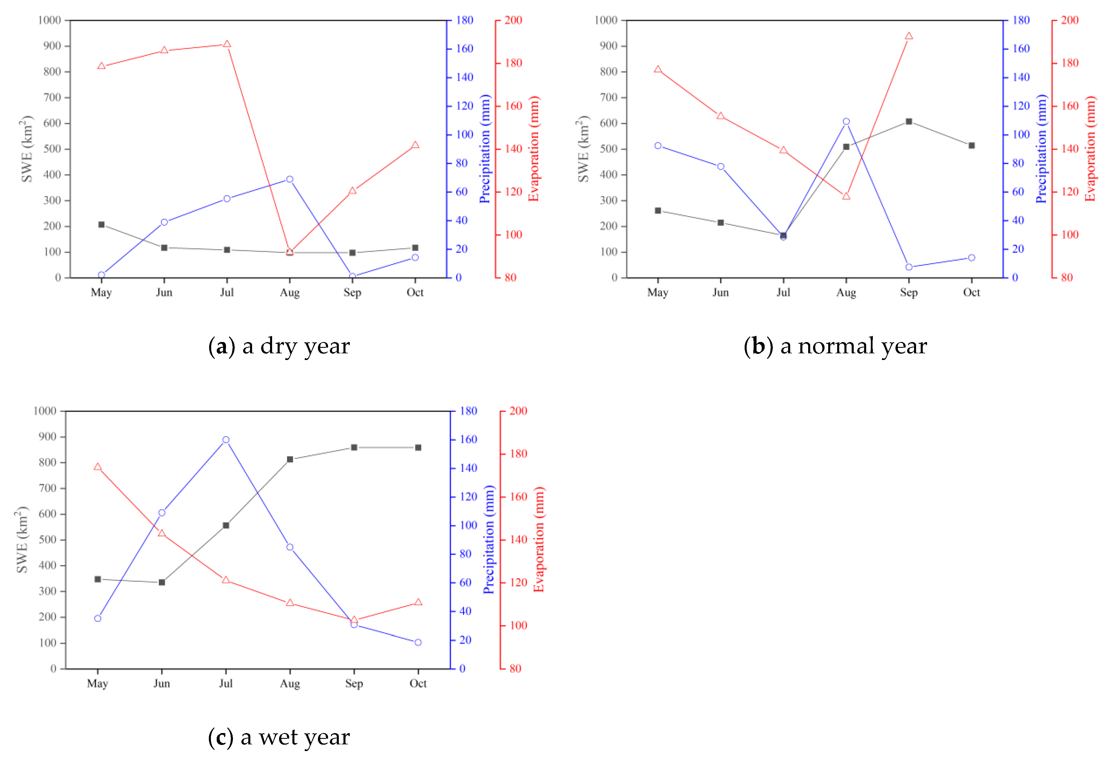
Our results show that the changing trends of the SWE of the top 10 largest connectomes were inconsistent during dry, normal, and wet years (Table 1). Further analysis found that, during the dry year, the changing trend of SWE was generally opposite to the changing trend of evaporation, and no positive correlation between SWE and precipitation was found (Figure 7a), indicating that evaporation is one of the main influencing factors of SWE in the dry year. In contrast, during the normal year, the changing trend of SWE was generally consistent with the changing trend of precipitation, and no negative correlation between SWE and evaporation was found (Figure 7b), indicating that precipitation is one of the main influencing factors of SWE in the normal year. During the wet year, the changing trend of SWE was generally opposite to the changing trend of evaporation, and no positive correlation between SWE and precipitation was found (Figure 7c), indicating that evaporation is one of the main factors affecting SWE in the wet year. Although there were many differences in the trend of SWE during different hydrological years, one trend was the same, that is, the SWE in May was higher than the corresponding value in June. This is because there were more replenishment water sources in May than in June. These extra water sources in May were snowmelt runoff and artificial water replenishment (i.e., recharged from irrigation and the farmland drainage network). Our results suggest that the surface water extent of the top 10 largest connectomes can be compared with precipitation and evaporation, in order to reveal the impact of precipitation and evaporation on the surface hydrology connectivity between water bodies. However, in terms of normal years, the components and spatial distribution of the top 10 largest connectomes in each month were different from the findings of our previous paper [15]. This may be due to the difference in temporal resolution (monthly average vs. 6–12 days) and spatial resolution (30 m vs. 10 m) of the dataset (JRC vs. Sentinel-1) used in the two studies.

5. Conclusions

This study demonstrated that the JRC Monthly Water History dataset derived from Landsat imagery is a valuable dataset for assessing the surface water dynamics, especially in ungauged areas. A remarkable advance of the dataset is that it greatly eliminated the impact of clouds on the quality of Landsat images. Using this dataset, geostatistical analysis was applied to quantify the spatiotemporal dynamics of surface hydrological connectivity under the influence of natural and human factors. Surface hydrological connectivity in the large multi-lake system changed along a gradient of wetness. During a dry year, due to lack of water input and geomorphological conditions, the surface hydrological connectivity along the W–E direction was better than that along the N–S direction. In normal and wet years, due to the combined effect of floods and river dam, the surface hydrological connectivity along the W–E direction was worse than that along the N–S direction. Overall, the surface hydrological connectivity in August, September, and October was better than that in May, June, and July. Overall, the surface hydrological connectivity in the east region was better than that in the central region, which in turn was better than that in the west region, and the surface hydrological connectivity in the rest of the region was poor.

Compared with other methods for the evaluation of hydrological connectivity, the main advantages of our approach are as follows: (1) it is completely objective; (2) it does not rely on ground measurement data such as water level and flow; (3) it outputs spatial and temporal distribution maps of hydrological connectivity; (4) it is economical and fast. While we expect that this approach can be applicable to other regions, two limitations should be noted. First, the JRC Monthly Water History dataset is a monthly composite dataset generated by Google on the basis of Landsat images. Although the overall accuracy of the dataset is very high, it actually reduces the temporal resolution of Landsat images. Second, the 30 m spatial resolution of the JRC Monthly Water History dataset applied in this study is still too coarse to detect details of surface hydrological connectivity. Overall, the temporal and spatial resolution of JCR data is lower than that of Sentinel-1 data; thus, it is not as good as Sentinel-1 data [15] in terms of displaying the details of surface hydrological connectivity. However, the advantage of JCR data is that it can be used directly without mastering professional remote sensing interpretation technology.

References

1. Pekel, J.-F.; Cottam, A.; Gorelick, N.; Belward, A.S. High-resolution mapping of global surface water and its long-term changes. Nature 2016, 540, 418–422. [Google Scholar] [CrossRef] [PubMed]
2. Lutz, A.F.; Immerzeel, W.W.; Shrestha, A.B.; Bierkens, M.F.P. Consistent increase in high ASIA’s runoff due to increasing glacier melt and precipitation. Nat. Clim. Chang. 2014, 4, 587–592. [Google Scholar] [CrossRef] [Green Version]
3. Micklin, P. The future Aral Sea: Hope and despair. Environ. Earth Sci. 2016, 75, 844. [Google Scholar] [CrossRef]
4. van Dijk, A.I.J.M.; Beck, H.E.; Crosbie, R.S.; de Jeu, R.A.M.; Liu, Y.Y.; Podger, G.M.; Timbal, B.; Viney, N.R. The millennium drought in southeast Australia (2001–2009): Natural and human causes and implications for water resources, ecosystems, economy, and society. Water Resour. Res. 2013, 49, 1040–1057. [Google Scholar] [CrossRef]
5. MacDonald, G.M. Water, climate change, and sustainability in the southwest. Proc. Natl. Acad. Sci. USA 2010, 107, 21256–21262. [Google Scholar] [CrossRef] [PubMed] [Green Version]
6. Trigg, M.A.; Michaelides, K.; Neal, J.C.; Bates, P.D. Surface water connectivity dynamics of a large scale extreme flood. J. Hydrol. 2013, 505, 138–149. [Google Scholar] [CrossRef] [Green Version]
7. Li, Y.; Zhang, Q.; Liu, X.; Tan, Z.; Yao, J. The role of a seasonal lake groups in the complex Poyang Lake-floodplain system (China): Insights into hydrological behaviors. J. Hydrol. 2019, 578, 124055. [Google Scholar] [CrossRef]
8. Liu, X.; Zhang, Q.; Li, Y.; Tan, Z.; Werner, A.D. Satellite image-based investigation of the seasonal variations in the hydrological connectivity of a large floodplain (Poyang Lake, China). J. Hydrol. 2020, 585, 124810. [Google Scholar] [CrossRef]
9. Tan, Z.; Wang, X.; Chen, B.; Liu, X.; Zhang, Q. Surface water connectivity of seasonal isolated lakes in a dynamic lake-floodplain system. J. Hydrol. 2019, 579, 124154. [Google Scholar] [CrossRef]
10. Lu, D.; Weng, Q. A survey of image classification methods and techniques for improving classification performance. Int. J. Remote Sens. 2007, 28, 823–870. [Google Scholar] [CrossRef]
11. Kartikeyan, B.; Majumder, K.L.; Dasgupta, A.R. An expert system for land cover classification. IEEE Trans. Geosci. Remote Sens. 1995, 33, 58–66. [Google Scholar] [CrossRef]
12. Yang, J.-B.; Xu, D.-L. On the evidential reasoning algorithm for multiple attribute decision analysis under uncertainty. IEEE Trans. Syst. Man Cybernetics Part A Syst. Hum. 2002, 32, 289–304. [Google Scholar] [CrossRef] [Green Version]
13. Bracken, L.J.; Croke, J. The concept of hydrological connectivity and its contribution to understanding runoff-dominated geomorphic systems. Hydrol. Process. 2007, 21, 1749–1763. [Google Scholar] [CrossRef]
14. Leibowitz, S.G.; Wigington, P.J., Jr.; Schofield, K.A.; Alexander, L.C.; Vanderhoof, M.K.; Golden, H.E. Connectivity of streams and wetlands to downstream waters: An integrated systems framework. J. Am. Water Resour. Assoc. 2018, 54, 298–322. [Google Scholar] [CrossRef] [PubMed]
15. Chen, Y.; Wu, L.; Zhang, G.; Xu, Y.J.; Tan, Z.; Qiao, S. Assessment of surface hydrological connectivity in an ungauged multi-lake system with a combined approach using geostatistics and spaceborne SAR observations. Water 2020, 12, 2780. [Google Scholar] [CrossRef]
16. Jiang, H.; He, C.; Luo, W.; Yang, H.; Sheng, L.; Bian, H.; Zou, C. Hydrological restoration and water resource management of Siberian Crane (Grus leucogeranus) stopover wetlands. Water 2018, 10, 1714. [Google Scholar] [CrossRef] [Green Version]
17. Yu, G.; Xu, M.; Sun, X.; Dong, L. Water Management Plan for the MNNR; The Drawing Times Press: Macao, China, 2009. (In Chinese) [Google Scholar]
18. Journel, A.G.; Kyriakidis, P.C.; Mao, S. Correcting the smoothing effect of estimators: A spectral postprocessor. Math. Geol. 2000, 32, 787–813. [Google Scholar] [CrossRef]
Figure 1. Location of the 1440 km2 Momoge National Nature Reserve (MNNR), China, and the network of lakes, rivers, and artificial ditches within the reserve. Data source: The United States Geological Survey (USGS) Landsat data.
Water 13 00497 g001
Figure 2. Example of how to calculate the geostatistical connectivity function (GCF) along the west–east (W–E) direction on the basis of the wet and dry binary state raster. The blue cells refer to wet cells, and the white cells refer to dry cells. The red lines with arrows mark the connection between pairs of wet cells, whereas the black lines with a symbol “×” and arrows mark the disconnection between pairs of wet cells. (a) Distance = 30 m, (b) Distance = 60 m, and (c) Distance = 90 m. Source: Figure reproduced from our previous paper [15].
Water 13 00497 g002
Figure 3. The relationship between geostatistical connectivity function (GCF) and maximum distance of connection (MDC) along the west–east (W–E) and north–south (N–S) directions of the multi-lake system in the Momoge National Nature Reserve (MNNR), China during different hydrological years. (a) W-E direction during a dry year, (b) W-E direction during a normal year, (c) W-E direction during a wet year, (d) N-S direction during a dry year, (e) N-S direction during a normal year, and (f) N-S direction during a wet year. Data source: The Joint Research Centre of the European Commission (EC JRC)/Google.
Water 13 00497 g003
Figure 4. Spatiotemporal distribution of the connectomes in Momoge National Nature Reserve, China during a dry year. Colors 1–10 in the legend refer to the top 10 largest connectomes, and color 11 refers to the remaining connectomes and isolated water bodies. Data source: EC JRC/Google.
Water 13 00497 g004
Figure 5. Spatiotemporal distribution of the connectomes in Momoge National Nature Reserve, China during a normal year. Colors 1–10 in the legend refer to the top 10 largest connectomes, and color 11 refers to the remaining connectomes and isolated water bodies. Data source: EC JRC/Google.
Water 13 00497 g005
Figure 6. Spatiotemporal distribution of the connectomes in Momoge National Nature Reserve, China during a wet year. Colors 1–10 in the legend refer to the top 10 largest connectomes, and color 11 refers to the remaining connectomes and isolated water bodies. Data source: EC JRC/Google.
Water 13 00497 g006
Figure 7. The relationship among surface water extent (SWE) of the top 10 largest connectomes, monthly mean precipitation, and monthly mean evaporation in the Momoge National Nature Reserve, China during (a) a dry year, (b) a normal year, and (c) a wet year. Data source: EC JRC/Google and China Meteorological Data Service Center.
Water 13 00497 g007