Analysis of Pore Water Pressure and Piping of Hydraulic Well

Abstract

This paper shows the results of a field appliance study of the hydraulic well method to prevent embankment piping, which is proposed by the Japanese Matsuyama River National Highway Office. The large-scale embankment experiment and seepage analysis were conducted to examine the hydraulic well. The experimental procedure is focused on the pore water pressure. The water levels of the hydraulic well were compared with pore water pressure data, which were used to look over the seepage variations. Two different types of large-scale experiments were conducted according to the installation points of hydraulic wells. The seepage velocity results by the experiment were almost similar to those of the analyses. Further, the pore water pressure oriented from the water level variations in the hydraulic well showed similar patterns between the experiment and numerical analysis; however, deeper from the surface, the larger pore water pressure of the numerical analysis was calculated compared to the experimental values. In addition, the piping effect according to the water level and location of the hydraulic well was quantitatively examined for an embankment having a piping guide part. As a result of applying the hydraulic well to the point where piping occurred, the hydraulic well with a 1.0 m water level reduced the seepage velocity by up to 86%. This is because the difference in the water level between the riverside and the protected side is reduced, and it resulted in reducing the seepage pressure. As a result of the theoretical and numerical hydraulic gradient analysis according to the change in the water level of the hydraulic well, the hydraulic gradient decreased linearly according to the water level of the hydraulic well. From the results according to the location of the hydraulic well, installation of it at the point where piping occurred was found to be the most effective. A hydraulic well is a good device for preventing the piping of an embankment if it is installed at the piping point and the proper water level of the hydraulic well is applied.

1. Introduction

The embankment on a river is made of soil as an important structure that prevents water from overflowing into the exclusion area [1]. KICT(Korea Institute of Civil Engineering and Building Technology) analyzed the type of collapse of embankments caused by floods. Among 758 cases of failure from 1987 to 2003, there were 300 cases of overflow destruction (about 39.6%), 295 cases of erosion (about 38.9%), and 87 cases of body instability (about 11.5%) [2]. When the water level of the river rises, the river embankment becomes unstable due to the development of the seepage line and the saturated area, which may cause a slope slide failure. Moreover, progressive backward erosion occurs due to piping on the foundation ground [3]. Im et al. (2006) [4] found that the stability of river banks is degraded because the outflow of rivers and the duration of flooding are rapidly increased due to extreme weather. Leakage from a river embankment refers to a phenomenon in which seepage water flows out to the inner site through the bode or the foundation of the embankment due to the rise in the water level in the exclusion site. At this time, leakage of the embankment causes the failure of the embankment when the seepage line reaches the slope of the embankment and the infiltrate flows out.

The leakage stability of an embankment has been studied through numerical analysis and experiments. Kim and Moon analyzed the shape and collapse mechanism of an embankment collapse by piping through the scale model test and large model test, and a hydraulic well was proposed and evaluated as a piping countermeasure (2017) [5]. Kim and Jo (1999) [1] investigated the leakage of an embankment using an electrical resistivity survey and evaluated the amount of leakage by using the weighted residual method. Jung et al. (2010) [6] performed a parametric analysis to examine the influence of the seepage coefficient in the seepage analysis of a river embankment. As for numerical analysis, Taylor and Brown (1967) [7] and Neuman and Witherspoon (1970) [8] applied the finite element method for the seepage of embankments. Uno et al. (1988) [9] conducted a basic study on stability by analyzing failure cases to evaluate the stability of a river embankment.

There are three main causes of leakage in river embankments. One cause is when the embankment’s width is small and the penetration distance of the permeable water is short. Another cause is when the embankment material contains a large amount of sandy or coarse soil with a high permeability coefficient, where a flow path may be created along the structure embedded in the embankment. On the other hand, leakage into the foundation of the embankment is called a piping phenomenon and becomes a problem for flood control. Therefore, sufficient countermeasures must be taken by reviewing the flow net, seepage pressure, and leakage amount.

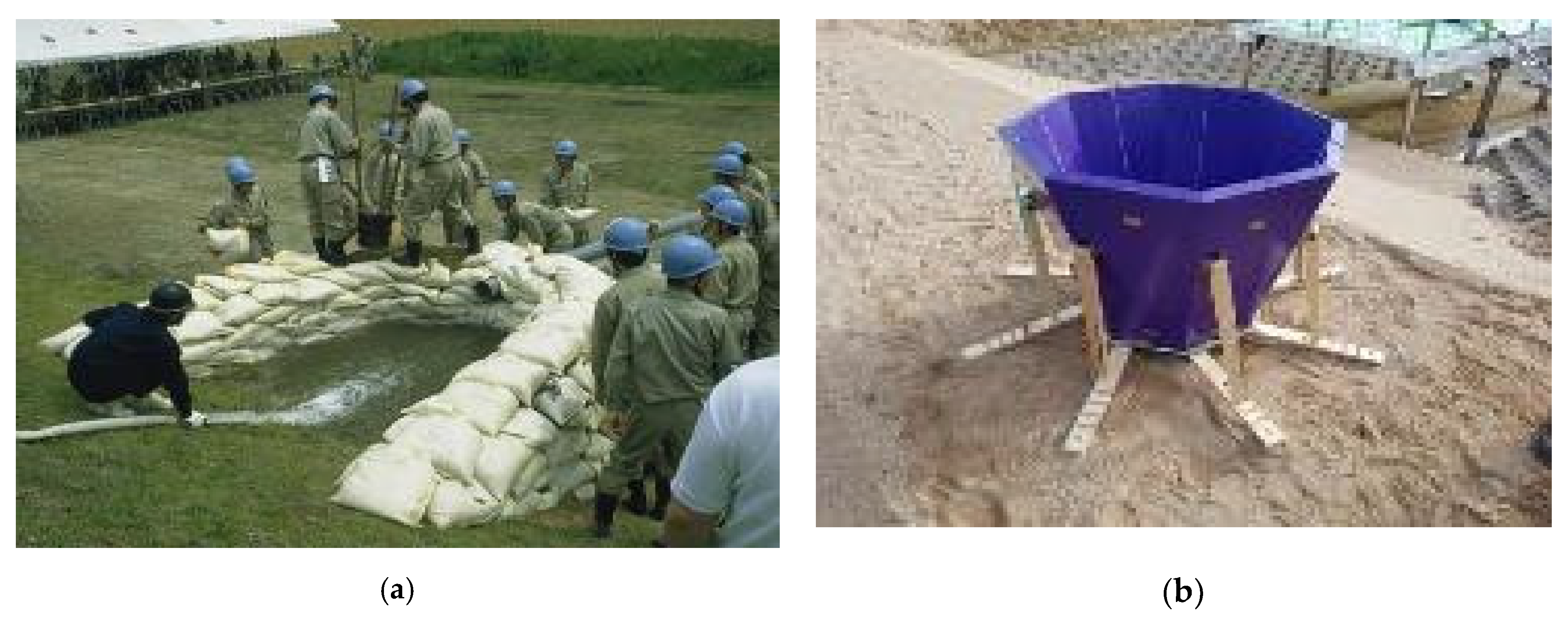
The Japanese Matsuyama River National Highway Office (2011) [10] proposes a hydraulic well as a countermeasure to prevent the piping of an embankment. This method is a technique that prevents piping by constructing a hydraulic well with a radius of 1.2~2.0 m using soil bags, and it reduces the seepage pressure by the water pressure in the hydraulic well.

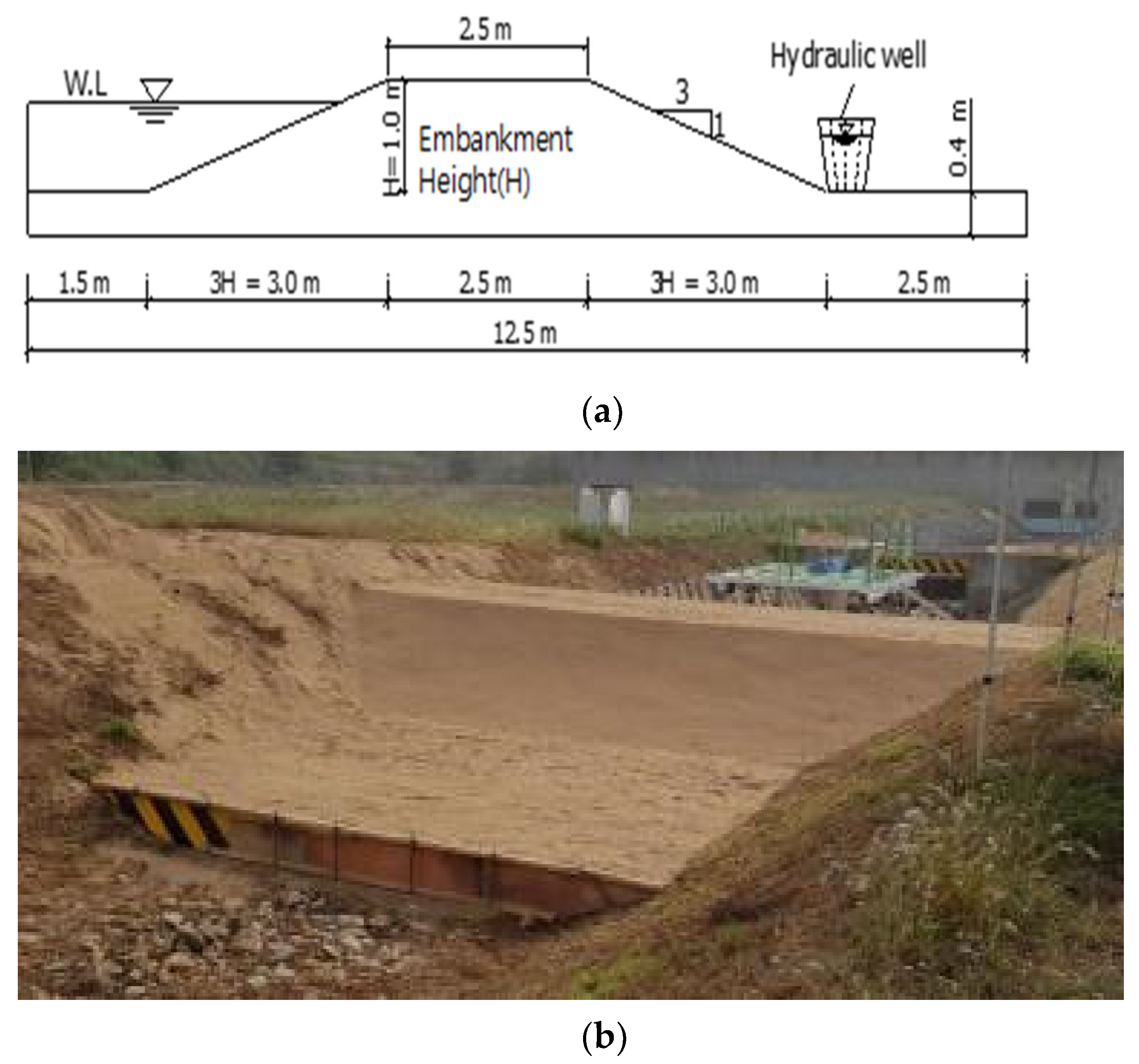
For this study, to verify the effectiveness of the hydraulic well to prevent piping, an experimental embankment that satisfies the Korea River Design Standard (2009) [11] was constructed with a height of 1.0 m, a width of the ridge of 2.5 m, and a slope of 1:3.

2. Seepage Behavior and Hydraulic Well

2.1. Seepage Behavior

The seepage analysis model includes steady and unsteady flow analysis, and unsteady flow analysis includes saturation and unsaturation analysis. The governing equation for seepage analysis is shown as Equation (1).

$$\frac{\partial h}{\partial x}\left(k_x\frac{\partial h}{\partial x}\right)+\frac{\partial h}{\partial y}\left(k_y\frac{\partial h}{\partial y}\right)+\frac{\partial h}{\partial z}\left(k_z\frac{\partial h}{\partial z}\right)+q_0=\alpha ·S_s·\frac{\partial h}{\partial t}$$

(1)

where $k_x$, $k_y$, and $k_z$ are the permeability coefficients in the direction of each coordinate axis, $k$ is the total head, $q_0$ is the specific flow rate, $s_s$ is the specific storage coefficient, and $\alpha$ is the coefficient of saturation.

The safety of piping is based on the results of the seepage analysis, and in this study, the stability of piping was analyzed by the method of the limit hydraulic gradient ($i_{cr}$), the same as Equation (2).

$$i_{cr}=\frac{{\gamma }_{sub}}{{\gamma }_w}= \frac{G_{s }-1}{1+e}$$

(2)

where $i_{cr}$ is the limit hydraulic gradient, ${\gamma }_{sub}$ is the unit weight of submerged soil ($\mathrm{k}\mathrm{N}/{\mathrm{m}}^3$), ${\gamma }_w$ is the unit weight of water ($\mathrm{k}\mathrm{N}/{\mathrm{m}}^3$), $G_s$ is the specific gravity of soil, and $e$ is the void ratio of soil.

2.2. Hydraulic Well

The Japanese Matsuyama River National Highway Office proposes a hydraulic well to prevent piping, as shown in Figure 1a. This construction method has a disadvantage in that it requires a lot of time and manpower as it is constructed by hand using soil bags. Therefore, in this study, a new hydraulic well was developed and manufactured to improve the workability and the seepage pressure distribution characteristics of the hydraulic well proposed in Japan. The developed hydraulic well was manufactured using stainless steel with an octagonal cone structure of 0.8 (height) × 0.77 m (inner diameter), as shown in Figure 1b. A total of 8 octagonal frames were assembled, and rubber packings were used to prevent leakage. Further, a lower pedestal supporting the octagonal frame was used.

3. Embankment Test and Pore Water Pressure of Hydraulic Well

3.1. Experimental Method

3.1.1. Embankment Soil

This test embankment was made of the riverbed soils of the Nakdong River in Andong, Korea. The engineering characteristics are shown in

Table 1. Engineering properties of experimental soils.

	Classification	Silty Sand
Characteristics
$G_s$		2.674
Plasticity Index		Non-Plasticity
Particle Size	#200 (%)	2.4
	Coefficient of Curvature ($C_g$)	0.9
	Coefficient of Uniformity ($C_u$)	3.6
	Unified Soil Classification System (USCS)	SP
Compaction	${\gamma }_{d,max}$(kN/${\mathrm{m}}^3$)	17.24
	Optimum Moisture Content (${\omega }_{opt}$ (%))	13.9
Shear Strength	Cohesion (kPa)	16.0
	Inner Friction Angle (Φ (°))	38.2

, and Figure 2 is the particle size distribution curve of the soil and the compaction curve by compaction used in the embankment test.

The soils were evaluated as SP(Poor Sand) according to the Unified Soil Classification System.

3.1.2. Construction of the Experimental Embankment

The large model test channel was located in the Andong River Experiment Center in Korea. The experiments were carried out on some sections in a straight waterway of 3.0 (bottom width) × 4.0 (waterway width) × 2.0 (waterway height) × 600 m (channel length).

Figure 3 shows a cross-sectional view of the experimental embankment. The height of the embankment was 1.0 m, and the width of the upper side was 2.5 m. The inclination of the slope of the riverside and the protected side was 1:3, which was built to satisfy the Korean River Design Standard (2009) [11]. Since piping occurs at the foot of the back slope of the protected side, a hydraulic well was placed at this point.

3.1.3. Pore Water Pressure Sensor Arrangement: Case 1 and Case 2

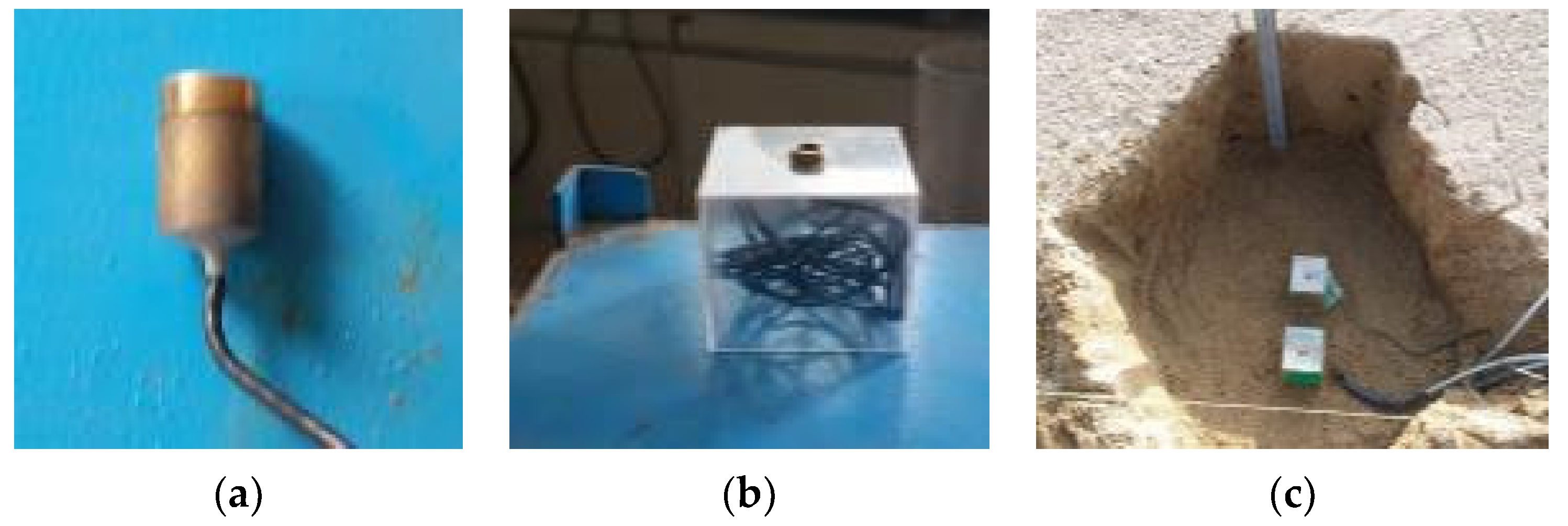
Figure 4 shows the installation process of the pore water pressure sensor. Figure 4a shows the pore water pressure sensor, and Figure 4b shows the sensor inside the acrylic case used in the experiment. As shown in Figure 4c, the pore water pressure sensors were buried at the planned location.

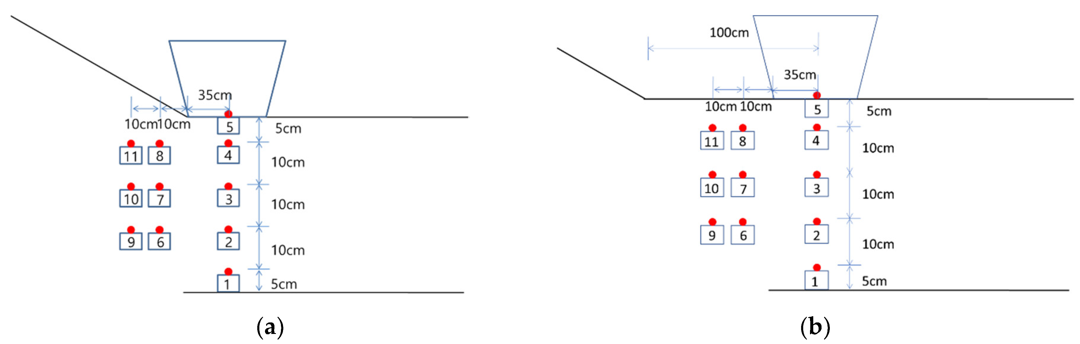
Figure 5 shows the buried position diagram of the pore water pressure sensors. There were two experimental cases. In case 1, the hydraulic well was installed 35 cm apart from the slope toe of the experimental embankment. As shown in Figure 5a, the pore water pressure sensors were placed at 10 cm intervals in the ground. Unlike case 1, in case 2, the hydraulic well was installed at a distance of 100 cm from the slope toe, and the arrangement of the pore water pressure sensors was the same as in case 1 (see Figure 5b).

3.1.4. Water Level of Hydraulic Well

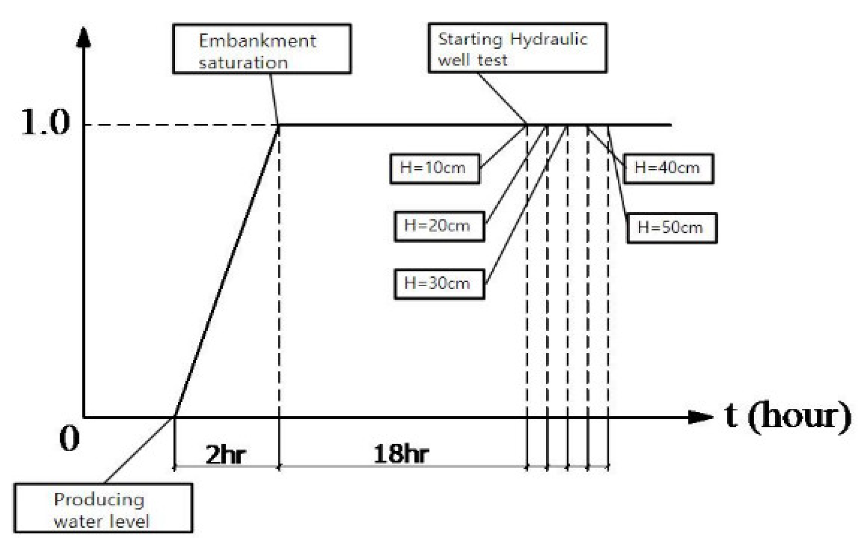
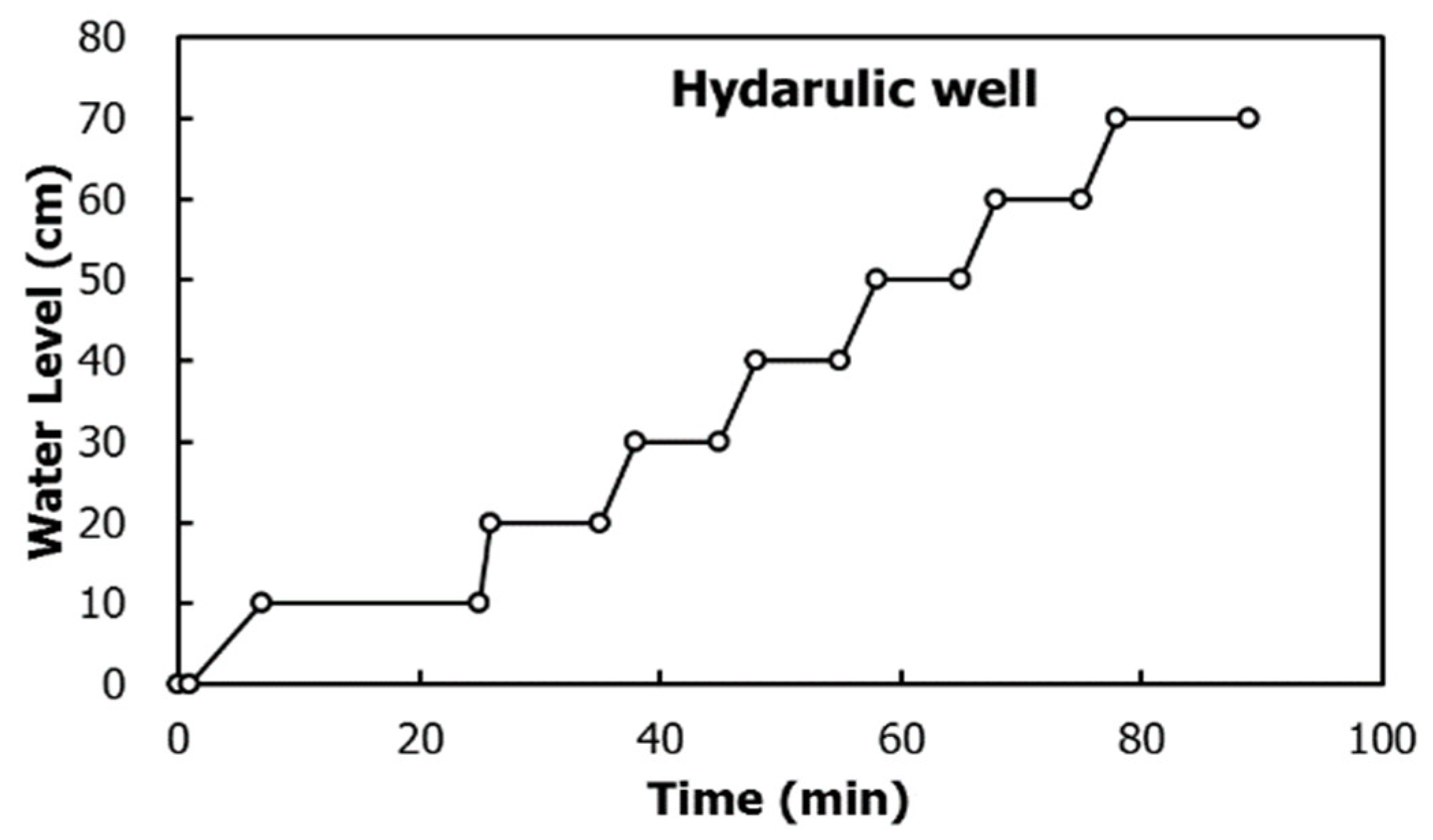
In this experiment, the hydrograph of the riverside is shown in Figure 6. After the embankment construction was completed, the full water level was produced for 2 h at the riverside. The hydraulic well experiment was performed after 18 h to saturate the embankment. Figure 7 shows the water level of the hydraulic well. It was increased by 10 cm every 10 min.

3.2. Experiment Results

3.2.1. Case 1

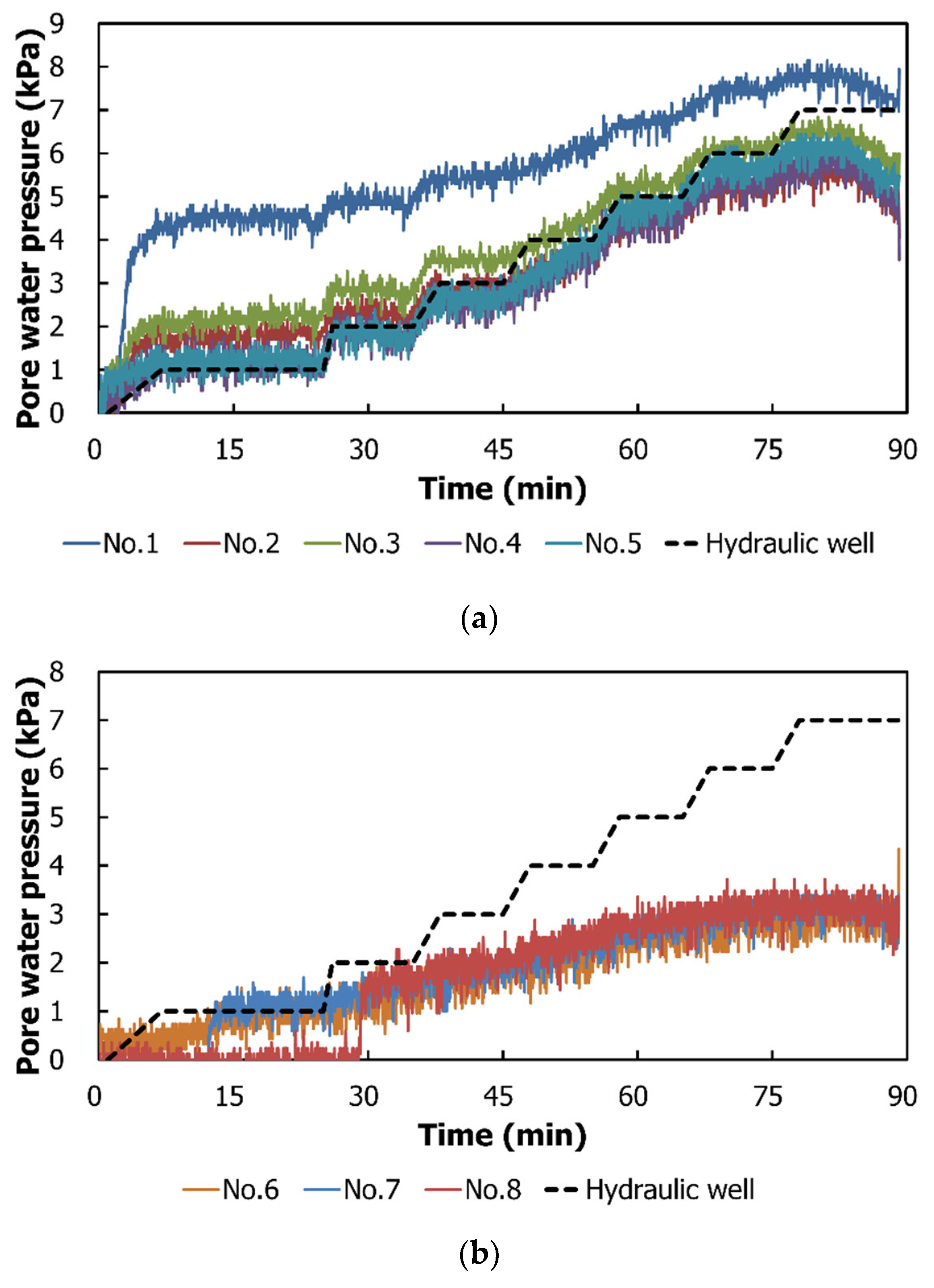
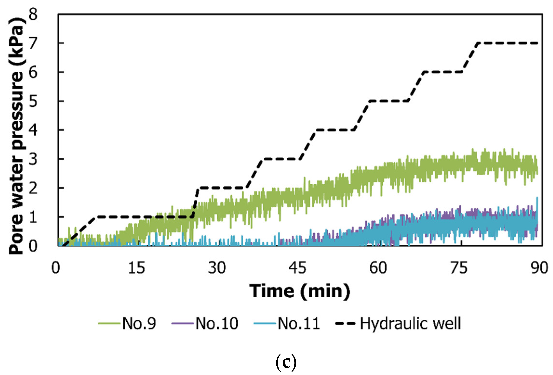
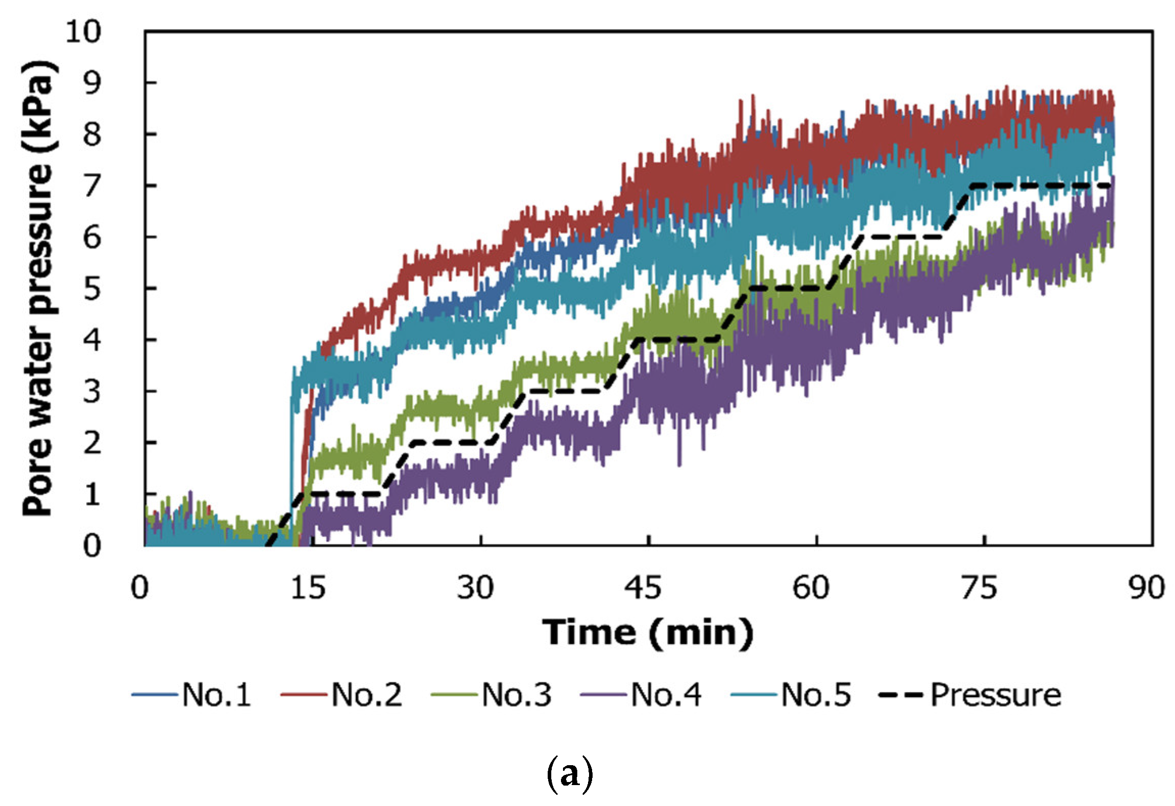
Figure 8 shows the experiment results of case 1. Figure 8a shows the variation in the pore water pressure by ground depth at the point where the hydraulic well was installed. The pore water pressure of sensor No.1 installed at 35 cm underground was analyzed to be about 3 kPa higher than the water level of the hydraulic well because the embankment was saturated and the phreatic line was generated. Therefore, closer to the ground surface, the difference becomes smaller between the water level of the hydraulic well and the pore water pressure.

Figure 8b shows the variation in the pore water pressure by ground depth at a point 45 cm horizontally apart from the hydraulic well. The No.6 sensor was installed at 25 cm underground, the No.7 sensor at 15 cm underground, and the No.8 sensor at 5 cm underground. The pore water pressures changed due to the variations in the water level in the hydraulic well. However, as can be seen in Figure 8a, the influence of the water level in the hydraulic well was reduced compared to the point where the hydraulic well was installed, and the pore water pressures were smaller than the water level in the hydraulic well.

Figure 8c shows the variations in the pore water pressures by ground depth at a point 55 cm apart from the hydraulic well, and it shows the same pattern as the pore water pressure distribution at the point separated by 45 cm (see Figure 8b).

3.2.2. Case 2

Figure 9 shows the experiment results of case 2. Figure 9a shows the variations in the pore water pressures by ground depth at the point where the hydraulic well was installed. The pore water pressure of sensor No.1 at 35 cm underground was estimated to be about 2~4 kPa higher than the water level of the hydraulic well because the embankment was saturated and the phreatic line was generated, the same as in case 1.

Figure 9b shows the variations in the pore water pressures by ground depth at the point 45 cm away from the hydraulic well. The No.6 sensor was installed at 25 cm underground, the No.7 sensor at 15 cm underground, and the No.8 sensor at 5 cm underground. The pore water pressure changed due to the variation in the water level in the hydraulic well. Further, the pore water pressure became smaller as it got closer to the surface due to the influence of the phreatic line. Moreover, the pore water pressure was generated smaller than the water level of the hydraulic well.

Figure 9c shows the variations in the pore water pressures by ground depth at a point 55 cm apart from the hydraulic well. Further, it shows the same pattern as the pore water pressure distribution at the point separated by 45 cm (see Figure 9b).

4. Numerical Analysis

4.1. Analysis Condition

4.1.1. Embankment Section and Mesh Size

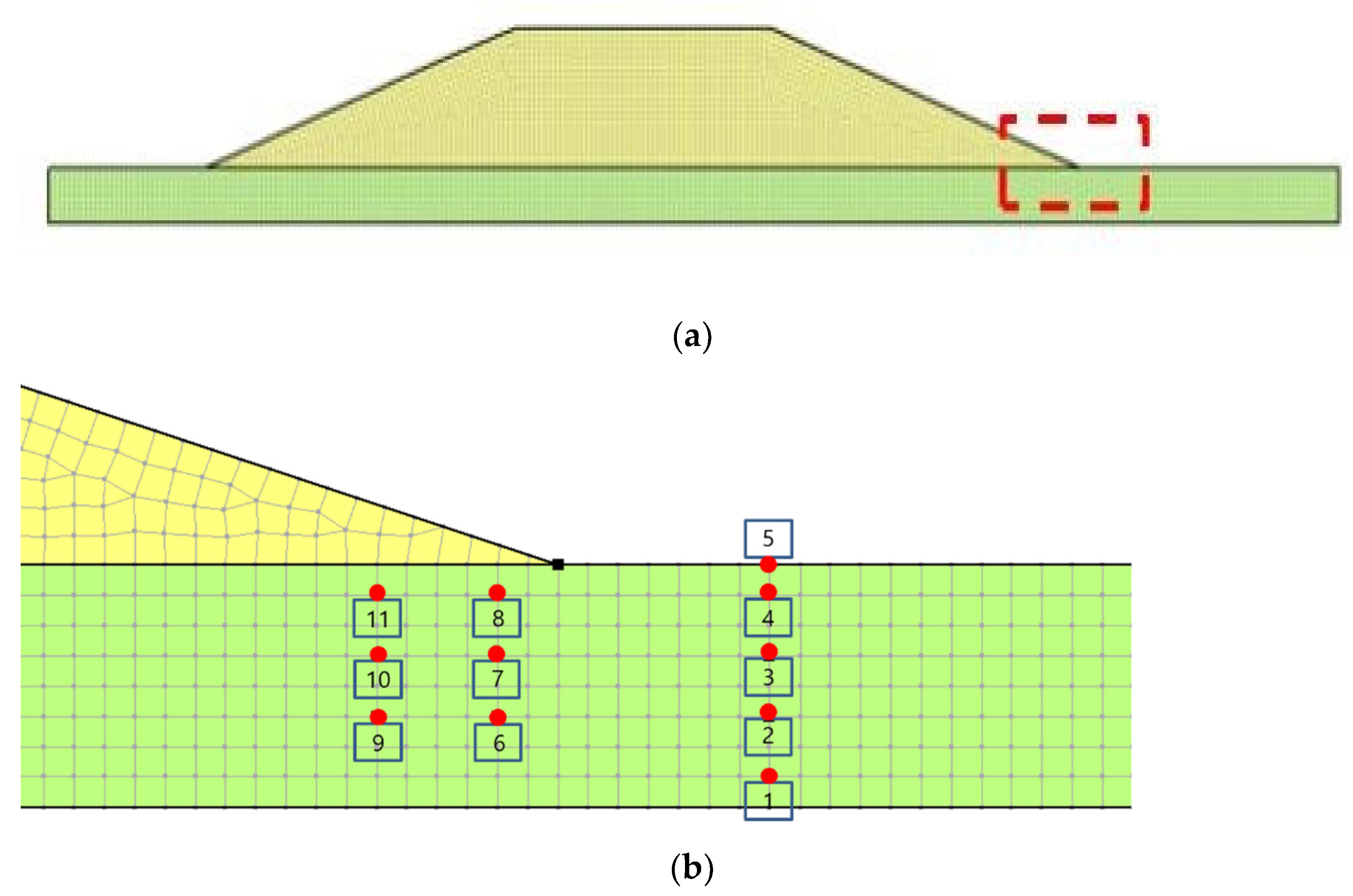
The cross-section for the seepage analysis was made the same way as the real test embankment, as shown in Figure 10a. For unsteady flow analysis, the mesh size has a great influence on the analysis results. The Korean River Design Standard suggests that the maximum size of the finite element for the embankment is limited to 1/10 or less of the embankment height to perform seepage analysis (KWRA, 2009) [11]. Therefore, in this study, the size of the finite element was 1/20 of the embankment height, 0.05 m (5 cm), as shown in Figure 10. Since it is an embankment without the piping guide part, a two-dimensional analysis was performed by applying the plane strain condition.

4.1.2. Soil Water Characteristic Curve and Water Level Conditions

Equation (3) by van Genuchten (1980) [12] was used for the soil water characteristic curve (SWCC).

$$\frac{\theta -{\theta }_r}{{\theta }_s-{\theta }_r}={[\frac{1}{1+{\left\{\alpha \left(u_a-u_w\right)\right\}}^n}]}^m$$

(3)

where ${\theta }_s$ is the saturated volumetric water content (${\mathrm{m}}^3/{\mathrm{m}}^3$), ${\theta }_r$ is the residual volumetric water content (${\mathrm{m}}^3/{\mathrm{m}}^3$), $\alpha$ is the reciprocal of the air entry value (1/m), $n$ is the coefficient related to the slope of the soil water characteristic curve, and $m$ is the slope-related coefficient at high levels of capillary absorption.

As for the unsaturated permeability coefficient, Equation (4) by van Genuchten (1980) [12] was applied in the same way as the soil water characteristic curve. The unsaturated permeability coefficient becomes a function of the capillary absorption capacity.

k_r = 〖[1 − {(αh)^(n − 1) ((1+〖αh)〗^n)^(−m))]〗^2/〖[1+〖(αh)〗^n]〗^(m/2)

(4)

where $h$ is the head of the negative pore water pressure (capillary absorption power), and $\alpha , \mathrm{n}, \mathrm{m}$ represent the curve fit coefficients.

Table 2. Unsaturated properties of soil.

Textural Class	Sand
Unified Soil Classification System (USCS)	SP
Saturated Volumetric Water Content, ${\theta }_r ({\mathrm{m}}^3/{\mathrm{m}}^3$)	0.045
Residual Volumetric Water Content, ${\theta }_s ({\mathrm{m}}^3/{\mathrm{m}}^3$)	0.43
Reciprocal of the Air Entry Value, $\alpha \left(1/m\right)$	14.5
Coefficient Related to the Slope of the Soil Water Characteristic Curve, $n$	2.68
Slope-Related Coefficient at High Levels of Capillary Absorption, $m$	0.627
Permeability Coefficient, $k_s (\mathrm{m}/\mathrm{s}$)	0.0009

shows the unsaturated properties of soil applied to the seepage analysis. SP was targeted, which is the sand shown in Table 1. The unsaturated properties of SP were quoted from the database presented by Carsel and Parrish (1988) [13].

The water level for the seepage analysis was applied in the same way as the water level waveform in the riverside (see Figure 5), and the water level in the hydraulic well was also applied in the same way as the experiment (see Figure 6).

4.2. Analysis Results

4.2.1. Experiment and Numerical Analysis Results of Case 1

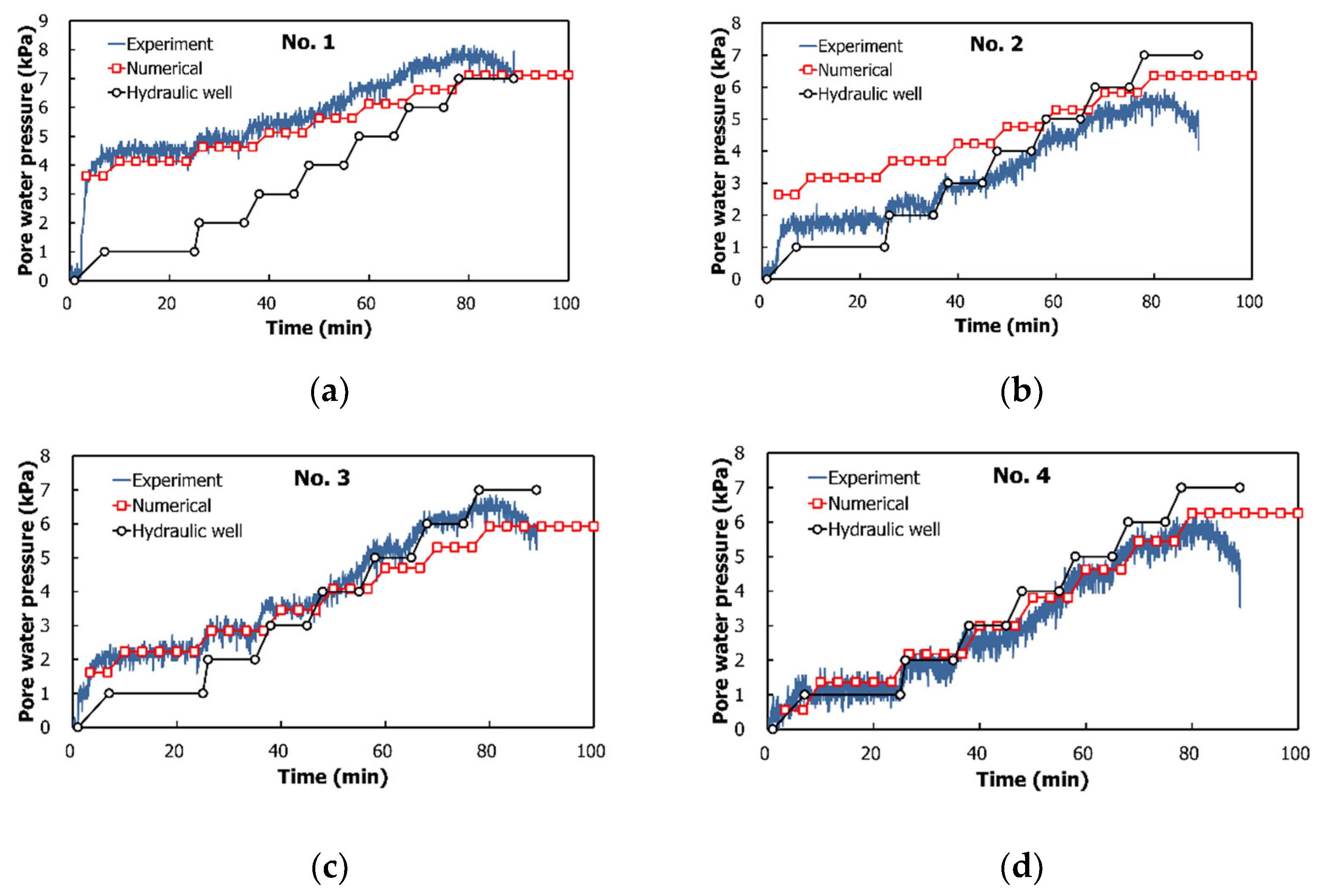
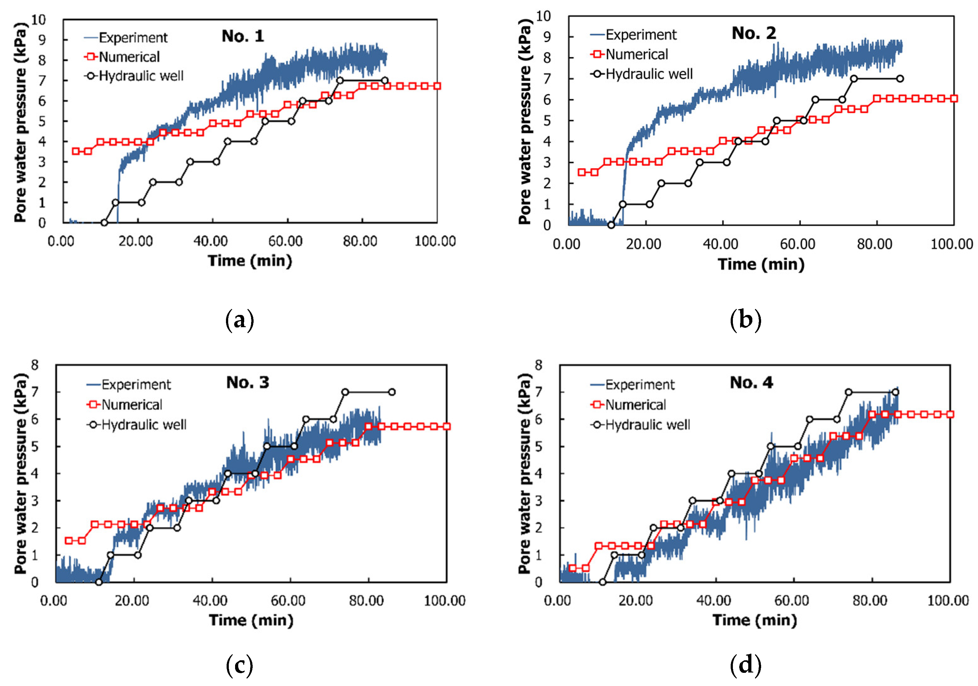
Figure 11 shows a comparison of the pore water pressure calculated through the experiment and numerical analysis at the point where the hydraulic well was installed. The pore water pressures through numerical analysis were based on a lapse of 20 h in the water level waveform of Figure 6. The No.1 sensor at 35 cm underground in Figure 11a showed almost similar behavior in the experiment and analysis. For the No.2 sensor at 25 cm underground in Figure 11b, the analysis result was estimated to be about 1 kPa higher than that of the experiment.

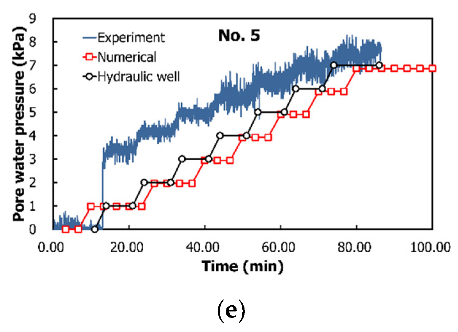
Figure 11c shows the results of the test and analysis of sensor No.3 at 15 cm underground, and Figure 11d shows the results of sensor No.4 at 5 cm underground. The results of sensor No.5 on the surface appear almost the same as the pore water pressures of the experiment, which means that the numerical analysis model is suitable for the seepage analysis (see Figure 11e).

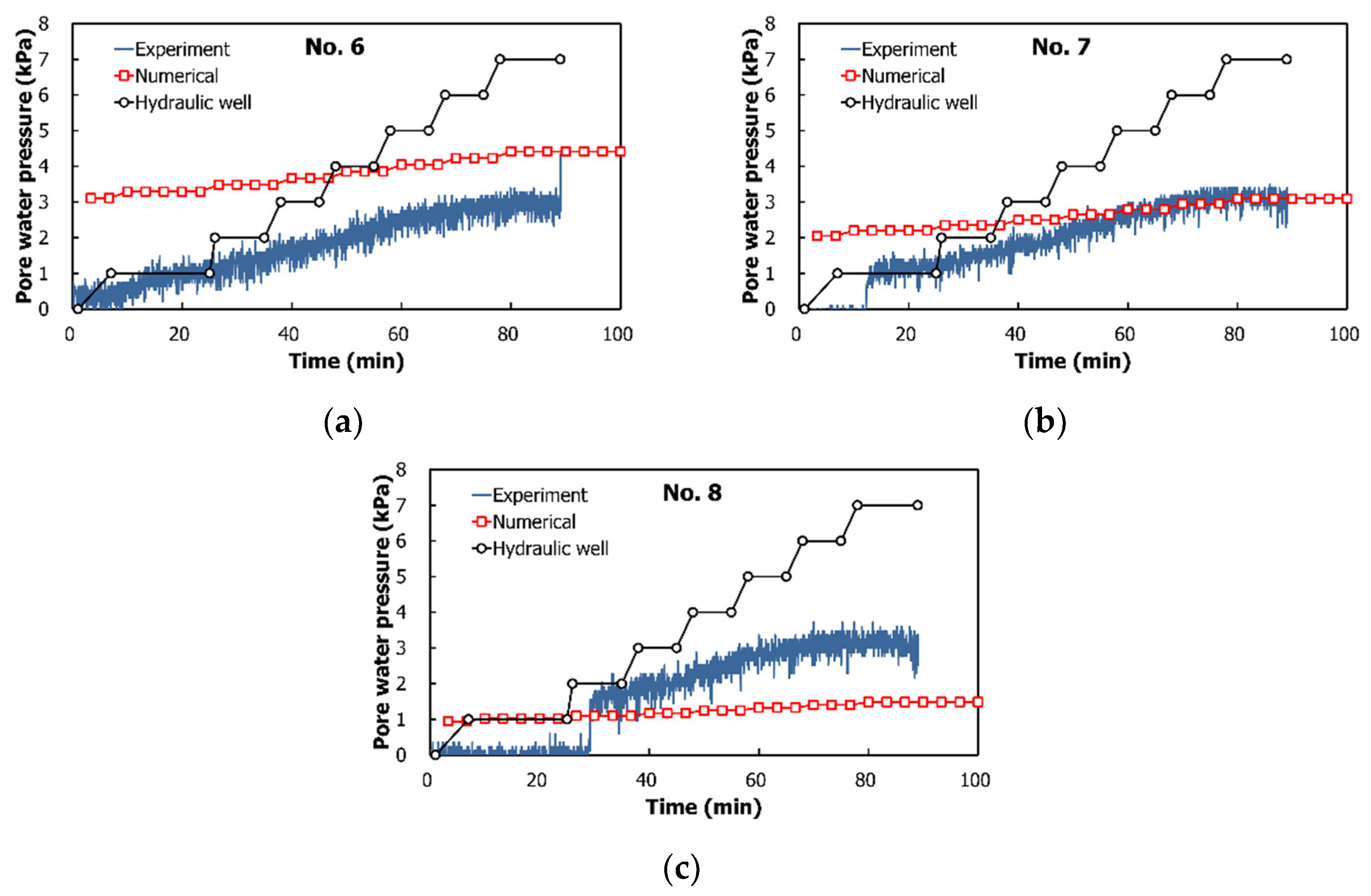
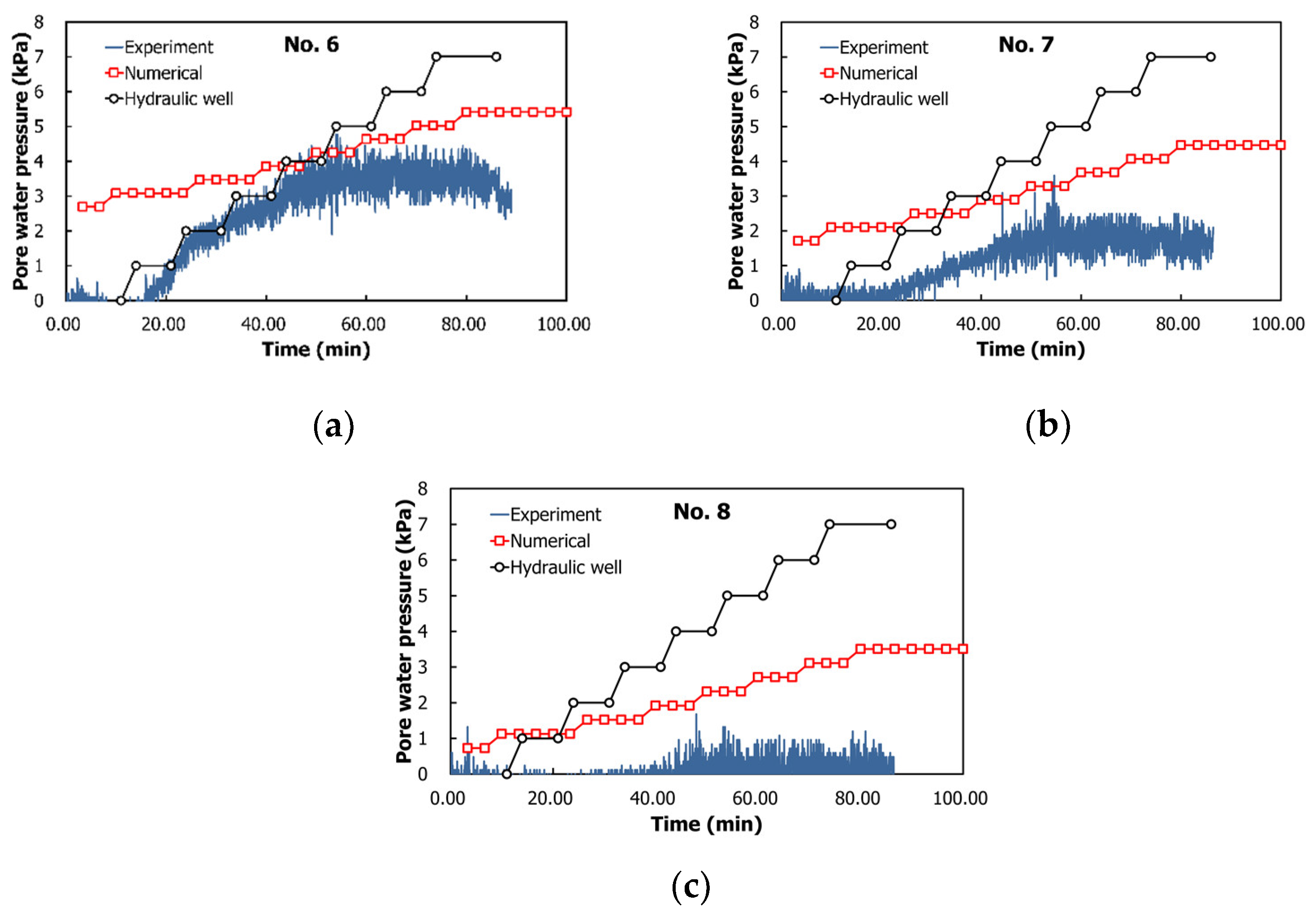
Figure 12 shows the pore water pressures 45 cm apart from the hydraulic well. For the No.6 sensor at 25 cm underground in Figure 12a, the analysis result was calculated about 2 kPa higher than that of the experiment. For the No.7 sensor at 15 cm underground in Figure 12b and the No.8 sensor at 5 cm underground in Figure 12c, the differences of the pore water pressures in the numerical analysis and experiment were reduced compared to the difference of sensor No.6.

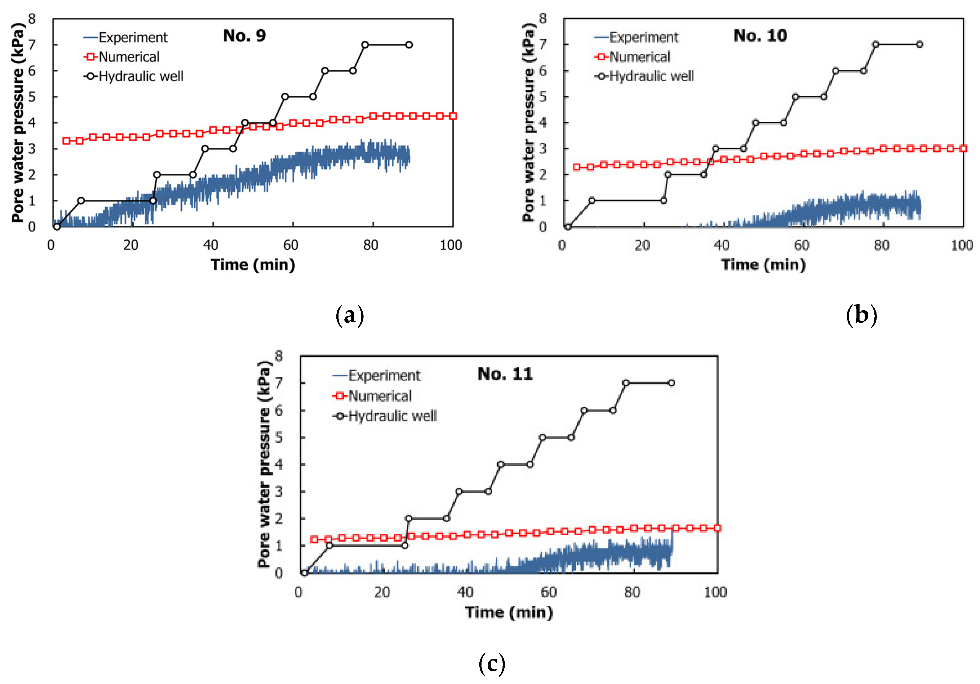
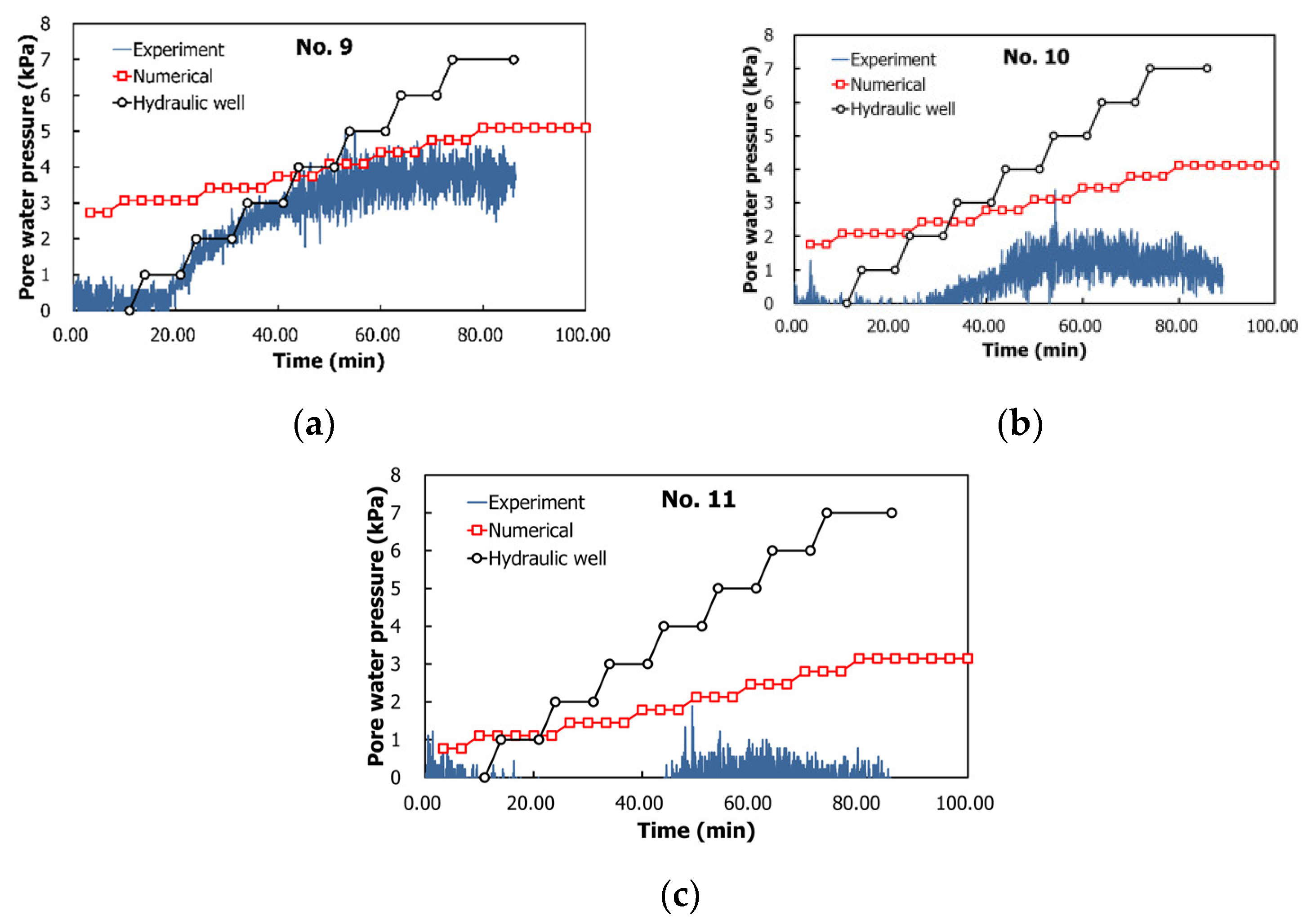
Figure 13 shows the pore water pressures 55 cm apart from the hydraulic well. For the No.9 sensor at 25 cm underground in Figure 13a, the numerical analysis result was initially calculated about 3 kPa higher than that of the experiment, but the difference decreased as the water level of the hydraulic well increased. Both the No.10 sensor at 15 cm underground in Figure 13b and the No.11 sensor at 5 cm underground in Figure 13c showed the same tendency as the No.10 sensor.

4.2.2. Experiment and Numerical Analysis Results of Case 2

Figure 14 shows the pore water pressures at the point where the hydraulic well was installed. The analysis results were based on the same criteria as in Section 4.2.1. For the No.1 sensor at 35 cm underground in Figure 14a and the No.2 sensor at 25 cm underground in Figure 14b, the pore water pressures in the experiment were estimated to be about 3 kPa higher than those of the analysis. The No.3 sensor at 15 cm underground in Figure 14c and the No.4 sensor at 5 cm underground in Figure 14d showed almost the same experimental and analysis results. The No.5 sensor showed higher experimental values than the numerical results (Figure 14e).

Figure 15 shows the pore water pressures 45 cm apart from the hydraulic well. The analysis result was calculated to be about 3 kPa higher than the pore water pressure of the experiment in the No.6 sensor at 25 cm underground (Figure 15a). The No.7 sensor at 15 cm underground (Figure 15b) and the No.8 sensor at 5 cm underground (Figure 15c) showed higher pore water pressures compared to the experimental values.

Figure 16 shows the pore water pressures 55 cm apart from the hydraulic well. The numerical analysis result was calculated as approximately 3 kPa higher than the experimental result in the early stage of the No.9 sensor at 25 cm underground (Figure 16a), but the difference decreased as the water level of the hydraulic well increased. Both the No.10 sensor at 15 cm underground (Figure 16b) and the No.11 sensor at 5 cm underground (Figure 16c) showed the same trend as the No.10 sensor.

5. Piping

5.1. Analysis Conditions

5.1.1. Embankment Section and Mesh Size

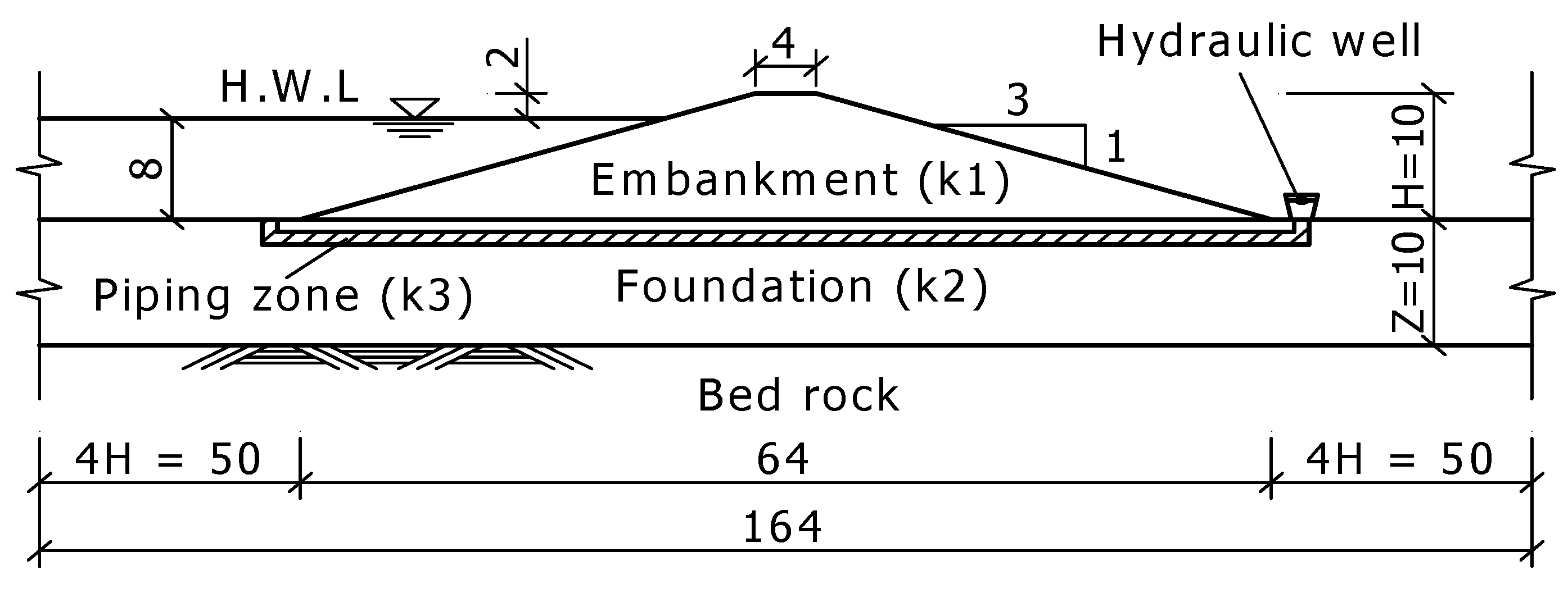
Piping is also greatly affected by the difference in the permeability coefficient between the embankment and the foundation ground. If the permeability coefficient of the foundation soil is larger than that of the embankment, the hydraulic gradient and the seepage velocity of the ground increase significantly [14]. Therefore, in this study, the permeability ratio ($k_1$/$k_2$) of the embankment ($k_1$) and the foundation ($k_2$) was considered as three conditions: 0.1, 1.0, and 10.0. Figure 17 is the cross-section of the embankment applied to the numerical analysis. K3 is the permeability coefficient of the piping guide part which is four times higher than that of the foundation soil.

In the same manner as the analysis of Section 4.1, the size of the mesh element was 1/10 of the height of the embankment, and the mesh was made to three dimensions. Further, the piping guide part, which has four times larger permeability than that of the embankment, was modeled and it was suggested by FEMA (2015) [15]. This is to verify the effectiveness of the hydraulic well after inducing the piping of the embankment.

5.1.2. Soil Water Characteristic Curve and Water Level Conditions

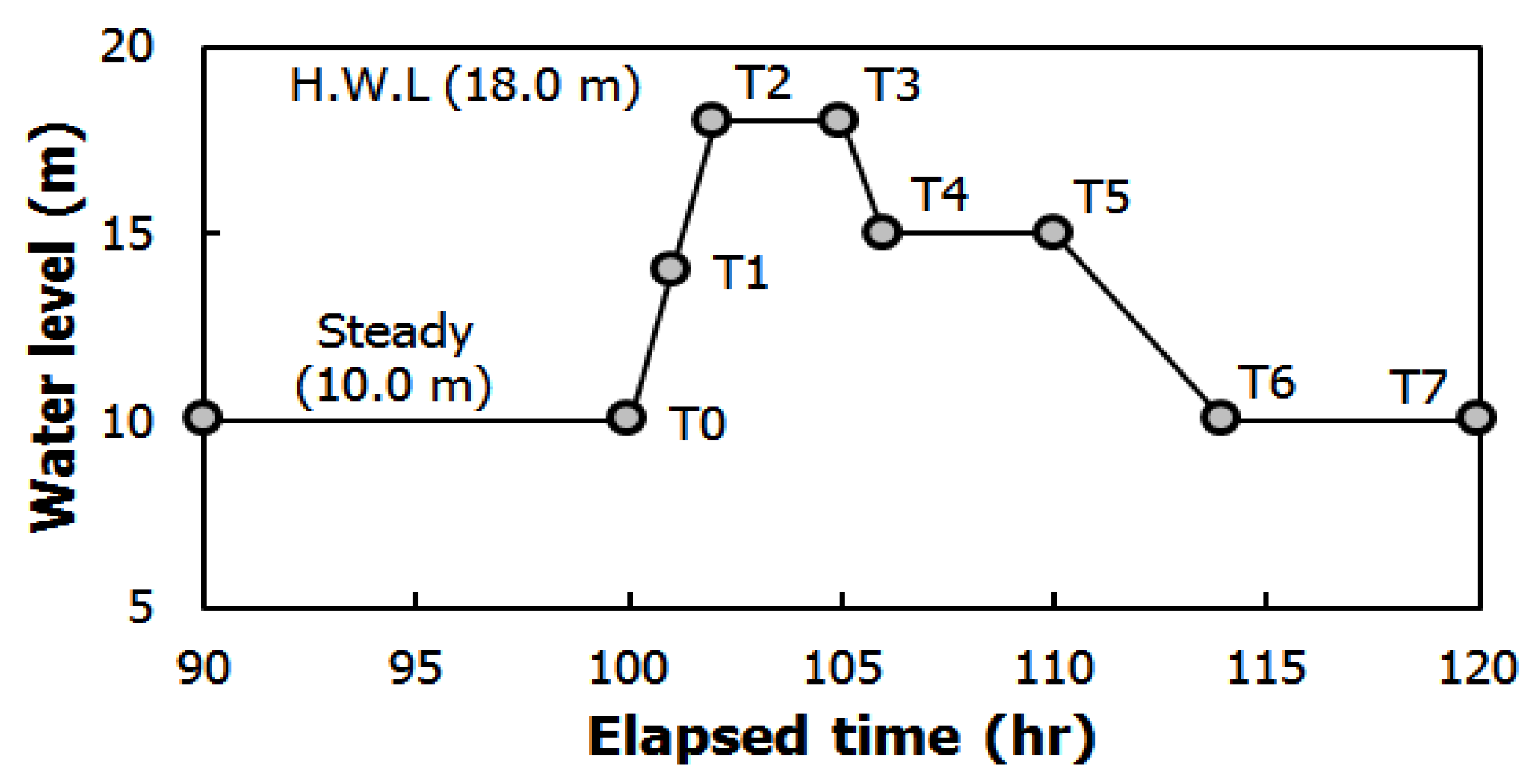
The unsaturated property of each soil applied to the seepage analysis is shown in Table 2 of Section 4.1.2 presented by Carsel and Parrish (1988) [13]. In order to examine the effectiveness of the hydraulic well, the water level curve in Figure 18 was used, which was induced from the Nakdong River embankment in Korea [5,14].

5.2. Analysis Results

5.2.1. Analysis by Water Level of Hydraulic Well

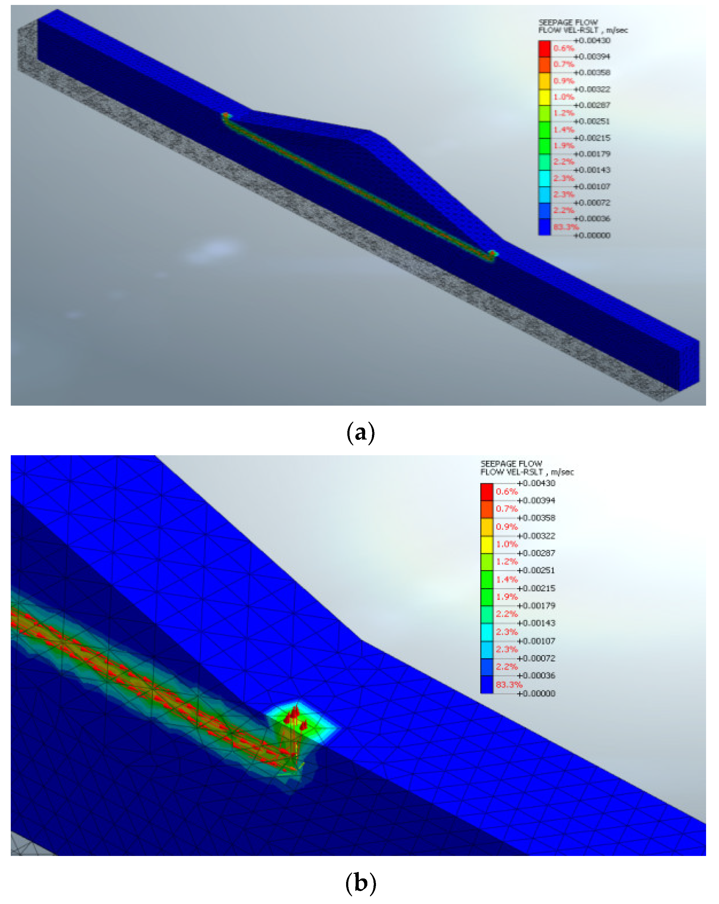
Figure 19 is the analysis results of the high water level (HWL) at 105 min in the water level waveform of Figure 18. It can be seen that the seepage water is concentrated in the piping guide part.

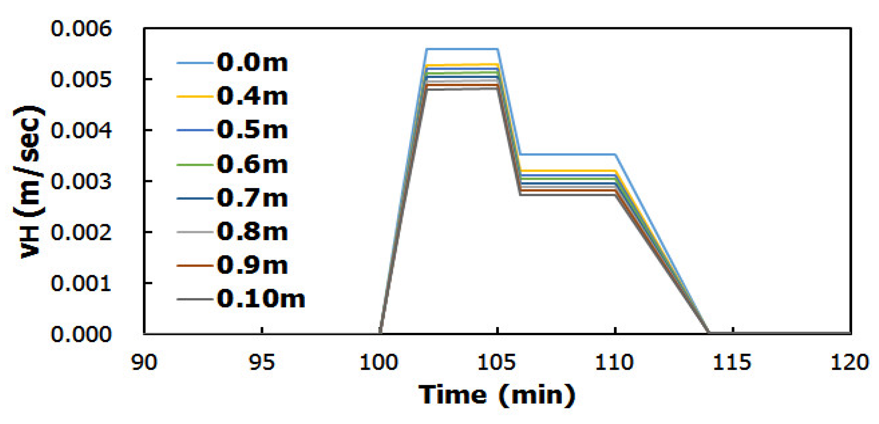
The effectiveness of the hydraulic well was evaluated by the seepage velocity at the point where piping occurred. Figure 20 shows the seepage velocity by the water level changes of the hydraulic well ($H_w$ = 0~1.0 m). The seepage velocity at the point of piping occurrence showed the same pattern as the water level waveform of the riverside shown in Figure 18. As the water level of the hydraulic well increased, the water level difference between the hydraulic well and the riverside decreased, so the seepage velocity decreased.

Table 3. Seepage velocity by the water level of the hydraulic well.

Time		Seepage Velocity (m/s) by the Water Level ( ${\mathit{H}}_{\mathit{w}}$) of the Hydraulic Well
h	s	0 m	0.4 m	0.5 m	0.6 m	0.7 m	0.8 m	0.9 m	1.0 m
100	360,000	0.00000	0.00000	0.00000	0.00000	0.00000	0.00000	0.00000	0.00000
101	363,600	0.00281	0.00265	0.00261	0.00257	0.00253	0.00249	0.00245	0.00241
102	367,200	0.00560	0.00528	0.00521	0.00513	0.00505	0.00497	0.00489	0.00481
105	378,000	0.00561	0.00529	0.00521	0.00513	0.00505	0.00497	0.00490	0.00482
106	381,600	0.00352	0.00320	0.00312	0.00304	0.00297	0.00289	0.00281	0.00273
110	396,000	0.00352	0.00320	0.00312	0.00305	0.00297	0.00289	0.00281	0.00273
114	410,400	0.00002	0.00002	0.00002	0.00002	0.00002	0.00002	0.00002	0.00002
120	432,000	0.00001	0.00002	0.00002	0.00002	0.00002	0.00002	0.00002	0.00002
$v_{max}\left(\mathrm{m}/\mathrm{s}\right)$		0.00561	0.00529	0.00521	0.00513	0.00505	0.00497	0.00490	0.00482
$\left(\frac{H_w=x}{H_w=0}\right)\times 100(\%)$		100.0	94.4	93.00	91.6	90.2	88.7	87.3	85.9

shows the seepage velocity by the water level ($H_w$ = 0~1.0 m) in the hydraulic well. In the water level waveform in Figure 18, the maximum values by time were compared. When there is no water level in the hydraulic well, the maximum seepage velocity was calculated as 0.00561 m/s, and when the hydraulic well level was 0.4 m, it was reduced to 0.00529 m/s. When applying the hydraulic well water level of 1.0 m, it was reduced by 85.9% from 0.00561 to 0.00482 m/s.

5.2.2. Analysis by Location of Hydraulic Well

Table 4. Seepage velocity by horizontal distance from piping point ($H_w$ = 0.7 m.

	Unapplied	Horizontal Distance from the Piping Point (m)
	None	−3	−2	−1	0	1	2	3
v (m/s)	0.0024	0.0024	0.0024	0.0128	0.0022	0.0129	0.0024	0.0024
$\left(\frac{v_{H_w}=x}{v_{none}}\right)\times 100(\%)$	100.0	100.0	100.0	526.8	90.1	530.9	100.0	100.0

shows the seepage velocity by horizontal distance from the point where piping occurred (the installation point of the hydraulic well). To examine the seepage velocity according to the horizontal distance from the point where piping occurred, the 0.7 m water level of the hydraulic well was applied. If the hydraulic well was not applied, the seepage velocity was calculated as 0.0024 m/s. If applying the hydraulic well water level at the point where piping occurred, it was reduced to 0.0022 m/s (90.1% reduction). However, when the hydraulic well was applied at a point 1.0 m horizontally from the point of piping, the seepage velocity increased by about five times to 0.0128~0.129 m/s. When the hydraulic well was applied to a point more than 1.0 m away from the point where piping occurred, it was found that it does not affect the seepage velocity at the point where piping occurs.

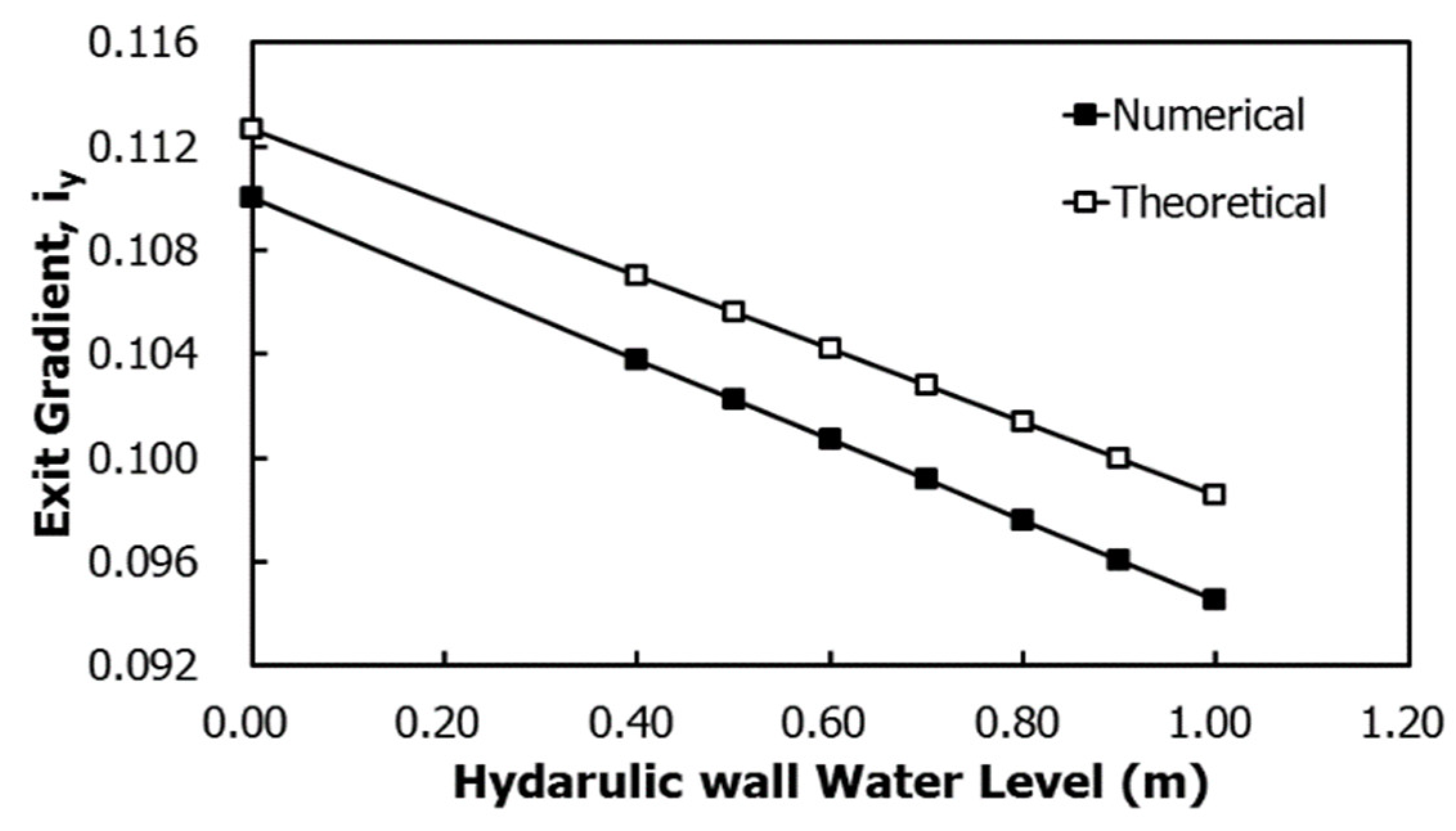
5.2.3. Hydraulic Gradients of Theory and Numerical Analysis

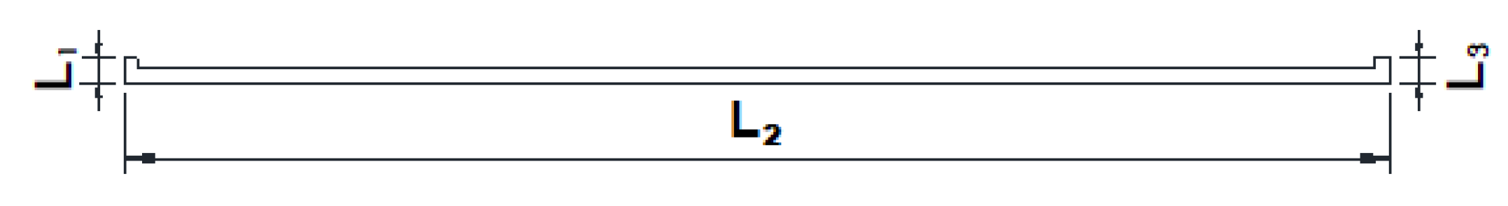
The hydraulic gradient results of the theory and numerical analysis were compared at the point where piping occurred. Figure 21 shows the streamline length for the piping guide part. The total length of the streamline is 71.0 m.

The theoretical hydraulic gradient ($i$) of the piping guide part is Equation (5). Δh is the difference in water level between the riverside and the protected side. The water level difference between the two sides is 8.0 m, and L represents the streamline length of the piping guide part of the embankment and is the sum of $L_1$(1.5 m), $L_2$ (68 m), and $L_3$ (1.5 m), shown in Figure 21.

$$i=\frac{\Delta h}{L_{total}}=\frac{\Delta h-H_{well}}{L_1+L_2+L_3}$$

(5)

Table 5. Theoretical hydraulic gradients according to the water level of hydraulic well.

${\mathit{H}}_{\mathit{w}\mathit{e}\mathit{l}\mathit{l}} \left(\mathbf{m}\right).$	${\mathit{L}}_{\mathit{t}\mathit{o}\mathit{t}\mathit{a}\mathit{l}} \left(\mathbf{m}\right)$	$\mathbf{\Delta }\mathit{h} \left(\mathbf{m}\right)$	$\mathit{i}$
0.0	71.0	8.00	0.1127
0.4		7.60	0.1070
0.5		7.50	0.1056
0.6		7.40	0.1042
0.7		7.30	0.1028
0.8		7.20	0.1014
0.9		7.10	0.1000
1.0		7.00	0.0986

shows the theoretical hydraulic gradient according to the hydraulic well level ($H_{Well}$) using Equation (5). As the water level of the hydraulic well increases, the difference in the water level between the riverside and the protected side decreases, so the theoretical hydraulic gradient is reduced by Equation (5).

Table 6. Hydraulic gradients of theory and numerical analysis.

${\mathit{H}}_{\mathit{w}\mathit{e}\mathit{l}\mathit{l}}\left(\mathbf{m}\right)$	Theoretical	Numerical
0.0	0.1127	0.1100
0.4	0.1070	0.1038
0.5	0.1056	0.1023
0.6	0.1042	0.1007
0.7	0.1028	0.0992
0.8	0.1014	0.0976
0.9	0.1000	0.0961
1.0	0.0986	0.0945

and Figure 22 show the results of the hydraulic gradients of the theory and numerical analysis, where the hydraulic gradient decreased linearly according to the water level of the hydraulic well.

6. Conclusions

This study aimed to improve the shortcomings of the hydraulic well method proposed by the Japanese Matsuyama River National Highway Office as a piping countermeasure. A new hydraulic well was developed to evaluate the seepage pressure, and the piping was analyzed through seepage analysis.

6.1. Comparison with Permanent Method

(1) The water defense methods such as hydraulic wells and installing soil bags refer to emergency treatment that is promptly performed so that the embankment does not collapse when there is an abnormality in the embankment during a flood. By installing a hydraulic well or stacking soil bags, the water pressure is weakened by reducing the difference in the water level between the riverside and the leak point of the embankment. Therefore, it is possible to prevent the collapse of the embankment. These construction methods are temporary measures and are different from permanent construction methods such as installing sheet piles at the bottom of the embankment or reinforcing the entire embankment.

(2) The hydraulic well method is known as a construction method that can be performed with the least cost and time among temporary water defense methods for embankments, but there was no engineering analysis for this. Therefore, by analyzing the pore water pressure change and piping behavior according to the water level change, the field applicability of the hydraulic well method was analyzed.

6.2. Pore Water Pressure

(1) There were two experimental cases, case 1 and case 2. For case 1, the hydraulic well was installed 35 cm apart from the slope toe of the experimental embankment.

For case 2, the hydraulic well was at a distance of 100 cm from the slope toe, and the arrangement of the pore water pressure sensors was the same as case 1.

(2) From the result of the pore water pressure of the embankment test and numerical analysis at the bottom of the hydraulic well, the pore water pressure results are almost the same as those at the ground surface; however, deeper from the surface, the larger pore water pressures of the numerical analysis were calculated compared to the experimental values. The results of case 1 and case 2 show the same patterns, which means that the numerical analysis model is suitable for seepage analysis.

(3) Even though the horizontal distance of case 2 was different from case 1, the characteristics of the pore water pressures were the same. When closer to the ground surface for both cases, the pore water pressure difference becomes smaller between the embankment test and numerical analysis.

6.3. Piping

(1) The piping effect according to the water level and location of the hydraulic well was quantitatively examined for the embankment with a piping guide part. As a result of applying the hydraulic well to the point where piping occurred, the hydraulic well with a 1.0 m water level reduced the seepage velocity by up to 86%. This is because the difference in the water level between the riverside and protected side is reduced, and it resulted in reducing the seepage pressure.

(2) From the results according to the location of the hydraulic well, installation of it at the point where piping occurred was found to be the most effective. When it was separated by 1.0 m horizontally from the point where piping occurred, inversely, the seepage velocity increased by about five times; further, when it was separated by 2.0 m, the seepage velocity was not affected by the distance from the point where piping occurred.

(3) As a result of the theoretical and numerical hydraulic gradient analysis according to the change in the water level of the hydraulic well, the hydraulic gradient decreased linearly according to the water level of the hydraulic well.

6.4. Hydraulic Well

(1) As the water level of the hydraulic well increased, the water level difference between the hydraulic well and the riverside decreased, so the seepage velocity decreased.

(2) A hydraulic well is a good device for preventing the piping of an embankment if it is installed at the piping point and if it is applied at the proper water level of the hydraulic well.

References

- Kim, K.; Jo, K. A Study on the Estimation of Leakage and the probing Leakage in the River Bank. Korean J. Korean Soc. Soil Ground Water Environ. 1999, 6, 213–217. [Google Scholar]
- KICT. The Final Report of the River Embankment Related Advanced Technology Development; Korea Institute of Civil Engineering and Building Technology: Gyeonggi-do, Korea, 2004; pp. 23–31, 68–78. [Google Scholar]
- KGS. Dam and Embankment Design and Construction Safety Management Technology; Goomi Book: Korea, 2012. [Google Scholar]
- Im, D.-K.; Yeo, H.-K.; Kim, K.-H.; Kang, J.-G. Suitability Analysis of Numerical Models Related to Seepage through a Levee. J. Korea Water Resour. Assoc. 2006, 39, 241–252. [Google Scholar]
- Kim, J.; Moon, I. Analysis of River Levee Failure Mechanism by Piping and Remediation Method Evaluation. J. Korea Acad. Ind. Coop. Soc. 2017, 18, 600–608. [Google Scholar]
- Jung, H.; Byun, Y.; Chun, B.; Choi, B.; Kim, J. Numerical Analysis for Integrity Evaluation of River Bank. J. Korean Geoenviron. Soc. 2010, 11, 19–26. [Google Scholar]
- Taylor, R.L.; Brown, C. Darcy flow solutions with a free surface. J. Hydraul. Div. 1967, 93, 25–33. [Google Scholar] [CrossRef]
- Neuman, S.P.; Witherspoon, P.A. Finite element method of analyzing steady seepage with a free surface. Water Resour. Res. 1970, 6, 889–897. [Google Scholar] [CrossRef] [Green Version]
- Uno, T.; Morisugi, H.; Sugil, T.; Nakano, Y. Stability evaluation of river levees on the basis of actual levee breachings. Doboku Gakkai Ronbunshu 1988, 1988, 161–170. [Google Scholar] [CrossRef] [Green Version]
- Office, M.R.N.H. Flood Prevention Handbook; Shikoku Regional Development Bureau: Shikoku, Japan, 2011.
- Association, K.W.R. River Design Standard; Ministry of Land, Transport and Maritime Affairs: Korea, 2009.
- Van Genuchten, M.T. A closed-form equation for predicting the hydraulic conductivity of unsaturated soils. Soil Sci. Soc. Am. J. 1980, 44, 892–898. [Google Scholar] [CrossRef] [Green Version]
- Carsel, R.F.; Parrish, R.S. Developing joint probability distributions of soil water retention characteristics. Water Resour. Res. 1988, 24, 755–769. [Google Scholar] [CrossRef] [Green Version]
- Kwon, K. An Improved Design Method of Levee Culvert Using 3D Seepage Analysis. Ph.D. Thesis, Kyunghee University, Seoul, Korea, 2007. [Google Scholar]
- FEMA. Evaluation and Monitoring of Seepage and Internal Erosion; Interagency Committee on Dam Safety (ICODS): Washington, DC, USA, 2015. [Google Scholar]
Figure 1.
Hydraulic well: (a) existing hydraulic well (2011); (b) developed hydraulic well.
Figure 2.
Particle size distribution and compaction curve of experimental specimens: (a) particle size distribution curve; (b) compaction curve.
Figure 3.
Section and panorama of experimental embankment: (a) section; (b) panorama.
Figure 4.
Installation process of the pore water pressure sensor: (a) sensor; (b) sensor inside the acrylic case; (c) sensors buried at the planned location.
Figure 5.
Buried position map of pore water pressure sensors: (a) case 1; (b) case 2.
Figure 6.
Hydrograph of the riverside.
Figure 7.
Hydrograph of the hydraulic well.
Figure 8.
Results of the pore pressure test (case 1): (a) hydraulic well installation point; (b) 45 cm separation site; (c) 55 cm separation site.
Figure 9.
Results of the pore water pressure test (case 2): (a) hydraulic well installation point; (b) 45 cm separation site; (c) 55 cm separation site.
Figure 10.
Location of pore water pressure sensors and mesh of embankment: (a) geometry and mesh; (b) pore water pressure sensor location.
Figure 11.
Comparison of pore water pressure of experiments and numerical analysis of case 1 (hydraulic well installation point): (a) No.1; (b) No.2; (c) No.3; (d) No.4; (e) No.5.
Figure 12.
Comparison of pore water pressure of experiments and numerical analysis of case 1 (45 cm separation site): (a) No.6; (b) No.7; (c) No.8.
Figure 13.
Comparison of pore water pressure of experiments and numerical analysis of case 1 (55 cm separation site): (a) No.9; (b) No.10; (c) No.11.
Figure 14.
Comparison of pore water pressure of experiments and numerical analysis of case 2 (hydraulic well installation point): (a) No.1; (b) No.2; (c) No.3; (d) No.4; (e) No.5.
Figure 15.
Comparison of pore water pressure of experiments and numerical analysis of case 2 (45 cm separation site): (a) No.6; (b) No.7; (c) No.8.
Figure 16.
Comparison of pore water pressure of experiments and numerical analysis of case 2 (55 cm separation site): (a) No.9; (b) No.10; (c) No.11.
Figure 17.
Cross-section of the embankment for numerical analysis (unit = −m).
Figure 18.
Water level waveform applied to the analysis.
Figure 19.
Analysis result of seepage velocity (HWL = 18.0, time = 105 h): (a) embankment view; (b) seepage velocity of piping guide part.
Figure 20.
Seepage velocity (m/sec) by the water level of the hydraulic well.
Figure 21.
Streamline length of piping guide part.