Determination of Internal Elevation Fluctuation from CCTV Footage of Sanitary Sewers Using Deep Learning

Abstract

The slope of sewer pipes is a major factor for transporting sewage at designed flow rates. However, the gradient inside the sewer pipe changes locally for various reasons after construction. This causes flow disturbances requiring investigation and appropriate maintenance. This study extracted the internal elevation fluctuation from closed-circuit television investigation footage, which is required for sanitary sewers. The principle that a change in water level in sewer pipes indirectly indicates a change in elevation was applied. The sewage area was detected using a convolutional neural network, a type of deep learning technique, and the water level was calculated using the geometric principles of circles and proportions. The training accuracy was 98%, and the water level accuracy compared to random sampling was 90.4%. Lateral connections, joints, and outliers were removed, and a smoothing method was applied to reduce data fluctuations. Because the target sewer pipes are 2.5 m concrete reinforced pipes, the joint elevation was determined every 2.5 m so that the internal slope of the sewer pipe would consist of 2.5 m linear slopes. The investigative method proposed in this study is effective with high economic feasibility and sufficient accuracy compared to the existing sensor-based methods of internal gradient investigation.

1. Introduction

Sewer pipes are designed to have a constant flow rate to transport sewage from cities to rivers or treatment areas. The main elements of the design are the pipe diameter and slope. There are not many options for pipe diameter because the manufacturing standards are set. However, the slope can be varied in a number of ways by the designer. To quantify the slope of the sewer pipe, the manhole-to-manhole gradient is represented as the ratio of the difference in pipe height to the straight-line distance, and per mil (1/1000, ‰) is used as the unit. The range of the slope of the sewer pipes in a flat city is generally <10‰, and the slope is calculated in great detail to two decimal places. Thus, a slight construction error can make the sewer pipe gradient disappear or even generate a counter gradient.

In addition, there can be problems inside sewer pipes as well. Even if the manhole-to-manhole gradient is perfectly constructed according to the design, the gradient inside a sewer pipe with a section length of 30–50 m is partially irregular. If a heavy 2.5 m long concrete pipe is laid on a foundation that has not been firmly compacted, the concrete pipe will naturally sink. Furthermore, if the slope is not precisely aligned, the slope of the foundation will not be uniform, and the sewer pipe will deflect over time due to leakage after completion of construction.

A gradient change inside the sewer pipe can be a major obstacle to stormwater transport. The lack of transport capacity of the downstream sewer pipe results in surcharge to the manhole or storm drain. There are various causes that can induce this lack of transport capacity, including lack of design capacity, steps due to damage, and excessive sedimentation (such as sediment inflow or concrete left from construction) [1,2]. In addition, the irregularity of the gradient inside the sewer pipe is also one of the causes of surcharge. The irregularity of the gradient inside the sewer pipe is accompanied by local deflection of the sewer pipe. Furthermore, congestion occurs in the deflected part during rainfall, and as the water fills upstream, a surcharge occurs in the manhole or storm drain. Because this internal irregularity is not revealed in the sewer pipe drawings or closed-circuit television (CCTV) survey reports, it is suspected to be one of the causes that induce flooding in some areas of the city where the sewer is designed properly and no abnormalities are found in the sewer pipe drawing. In addition, local deflection is also a cause of sedimentation and odor generation, as well as river pollution because it raises the combined sewer overflow concentration [3,4].

Because the irregularity of the gradient inside the sewer pipe causes the problems described above, many studies have been conducted to accurately investigate the problems inside the sewer pipe. Some examples are related to profiling inside the sewer pipe using instruments such as lasers [5,6], ultrasonic devices [7,8], sonar [9], and CCTV with electronic tilt meter [10], which have been used to construct a profile of the inside of a sewer pipe. These types of precise instruments exhibit excellent performance compared to CCTV investigations. However, these approaches have not been widely applied because they require significant time and have a high equipment cost.

The recent development of image recognition techniques using deep learning has enabled quantitative information to be extracted from images or videos. Deep learning entails a class of algorithms that learn representations of data with multiple levels of abstraction via multiple processing layers [11]. Layers of features, which are not designed by engineers of a specific field, are used for general-purpose learning. Some studies have automatically detected defects from CCTV footage using these advantages [12,13,14], but they were limited to functional defects inside pipes such as cracks, deposits, and tree roots. These studies used software applications to investigate the types of defects that can be identified using existing CCTVs.

Obtaining new information from existing CCTV footage increases the utilization of CCTVs. In general, CCTV surveys reveal a variety of information, but the water level or flow rate is only determined via a flow meter or water level meter. The roles of CCTV and flow meters are different. However, methods such as particle image velocimetry (PIV) and large-scale particle image velocimetry (LSPIV) [15,16] use video inspection to measure the stream flow velocity from images.

Although the image processing of sewer pipe footage is difficult owing to the dark environment and contamination, Ji et al. [17] proposed a method for extracting water level and flow rate from videos taken inside sewer pipes; particularly, this method automatically recognizes the water level using deep learning and calculates the flow rate based on geometrical principles and Manning’s equation. Using this principle, the water level of entire sewer pipe sections can be measured from CCTV footage.

The water level can be used to investigate local deflection due to a gradient change inside the sewer pipe. If the gradient of the sewer pipe is constant, the water level will also be constant. In contrast, the water level will be high where the sewer pipe is deflected and low where it is raised. Changes in the elevation or slope of the sewer pipe can be recognized by the relative fluctuation of the water level. Although this information can be roughly identified by an investigator through CCTV footage, it cannot be quantified. This study demonstrated the process of quantitatively estimating the gradient inside the sewer pipe from CCTV footage using the aforementioned principle.

2. Materials and Methods

CCTV footage of the sewer pipe 2049-500 (diameter 450 mm, length 40.03 m, slope 2.5‰, reinforced concrete pipe) located in Seoul, South Korea was taken from the downstream manhole to the upstream manhole. This video was in MP4 format with 19,933 frames in total, and it had a recording time of 5 min 34 s, a frame rate of 30, a resolution of 1280 × 720, and a size of 263 MB. The tools used to analyze this video were MATLAB’s deep learning toolbox, image processing toolbox, and computer vision toolbox.

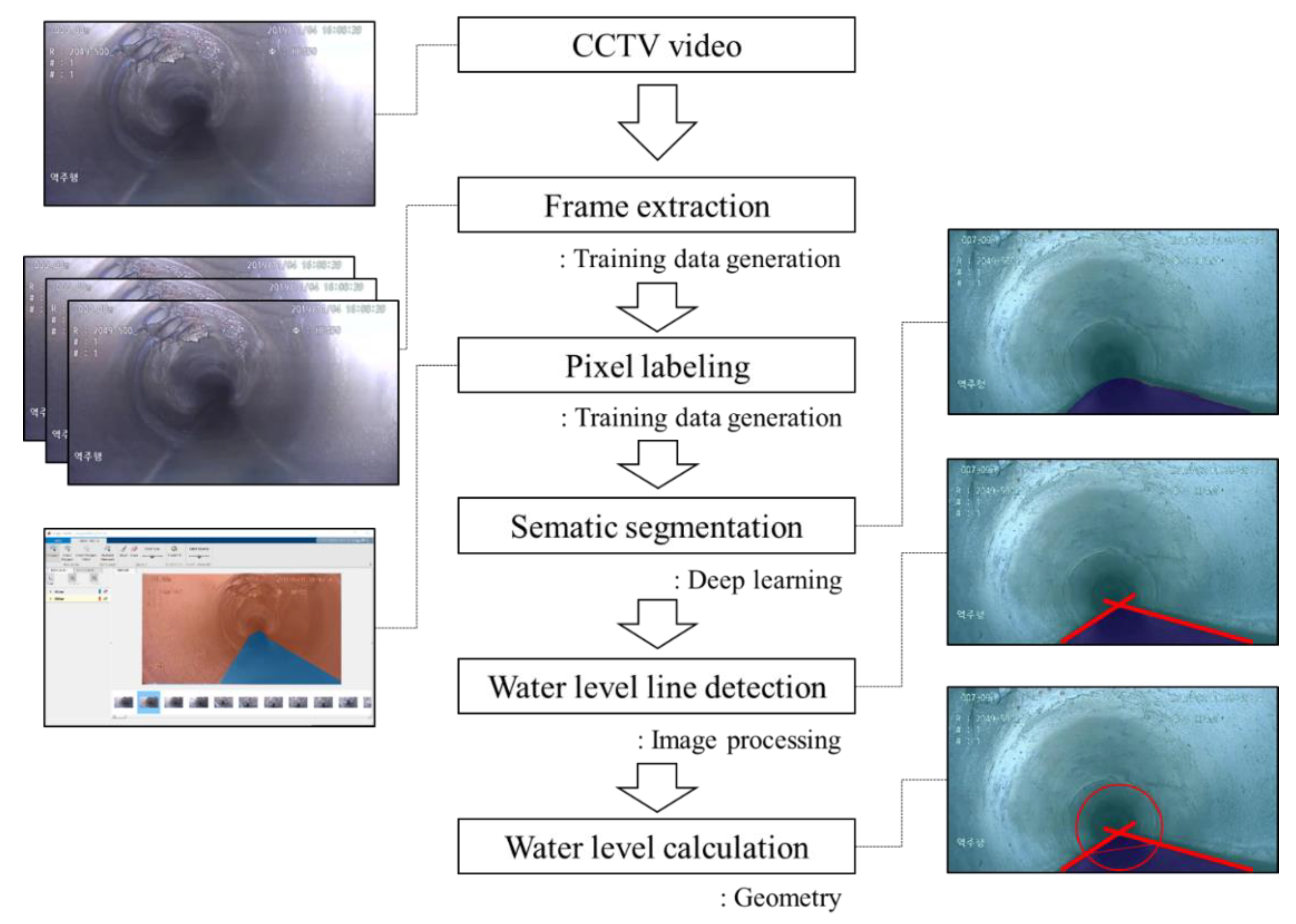
Figure 1 shows the overall process of this study. Deep learning starts with creating training data. By decomposing CCTV into frames and extracting frames relatively evenly from all sections, 283 training images were selected. These images were divided into a water area and a pipe area by pixel labeling. 60% of the labeled training image data were utilized for training, while 20% was used for verification and was used 20% for testing. Moreover, images were randomly separated. A new network for deep learning was created using DeepLab v3+ based on pre-trained ResNet-18 for fitting the image size and label. ResNet-18 is a convolutional neural network (CNN) that classifies images [18], and DeepLab v3+ is a CNN designed for labeling images [19]. An optimization algorithm, stochastic gradient descent with momentum (SGDM) [20], was used for training. The learning rate was reduced by a factor of 0.3 every 10 epochs and the network was tested against the validation data every epoch. Further, mini-batch size of 2 was used to reduce the memory usage during training [21]. Training was repeated 2190 times in total in 30 epochs for 45 min, which ended with 98% accuracy. The training process was calculated using the GPU NVIDIA Quadro P5000 16GB. CCTV footages were divided into water and pipe areas through this network, and this process is called semantic segmentation.

When semantic segmentation is performed, each frame in the image creates a matrix assigned only by the label of water or pipe, and this matrix is converted into a binary image with water = 1 and pipe = 0. When the results of semantic segmentation for each frame are examined, misrecognized areas are found. CCTV video recording focuses on the connection pipe and joint by turning the line of sight, in addition to moving straight through the inside of the sewer pipe. Although these parts are automatically excluded from recognition, corrections are required for the error parts due to possible recognition errors. To remove the noise, such as that caused by water droplets on the frame, objects with 40,000 or less pixels were all deleted. When the errors were removed, only the area corresponding to water remained, and an edge was obtained from this area.

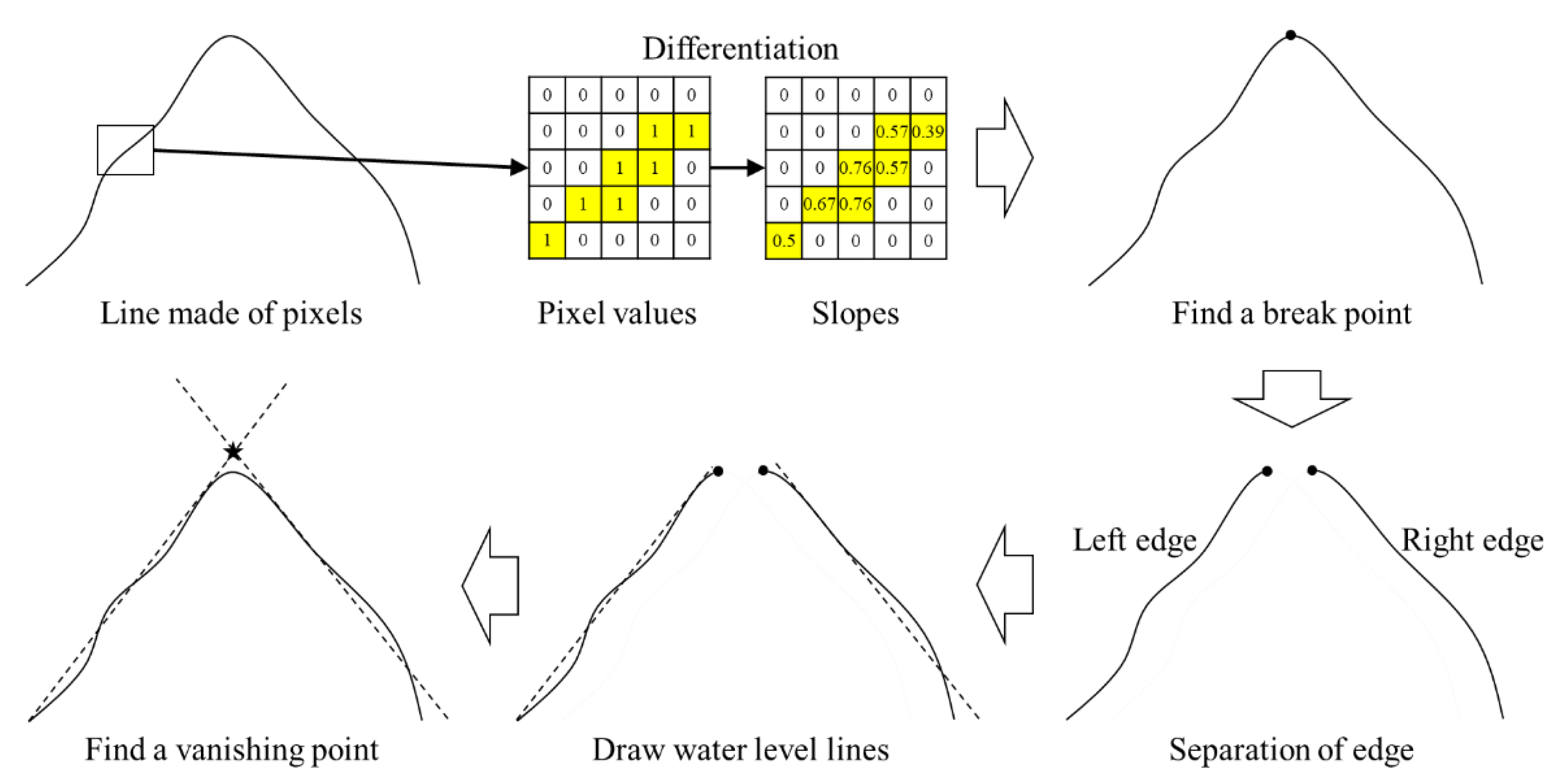
This edge was a mountain-shaped line, as shown in Figure 2, and the line was differentiated. However, because images are pixels, they cannot be differentiated. Instead, using the features of the pixel, a 5 × 5 matrix was extracted around a data point, and the slope was extracted by obtaining a linear equation from the data points by the least squares method. Based on the slope value, a break point that forms the reference of the left and right edges can be obtained. Based on this break point, two linear equations were obtained from the left and right edges by the least squares method. These equations correspond to the water level lines of the sewer, and the point where the two lines meet is the vanishing point. An imaginary circle was drawn around the vanishing point, from which the distance (d) between the chord and the circle was obtained, and then the water level was further calculated in proportion to the diameter of the sewer pipe [17]. This process was applied to the entire CCTV footage.

3. Results and Discussion

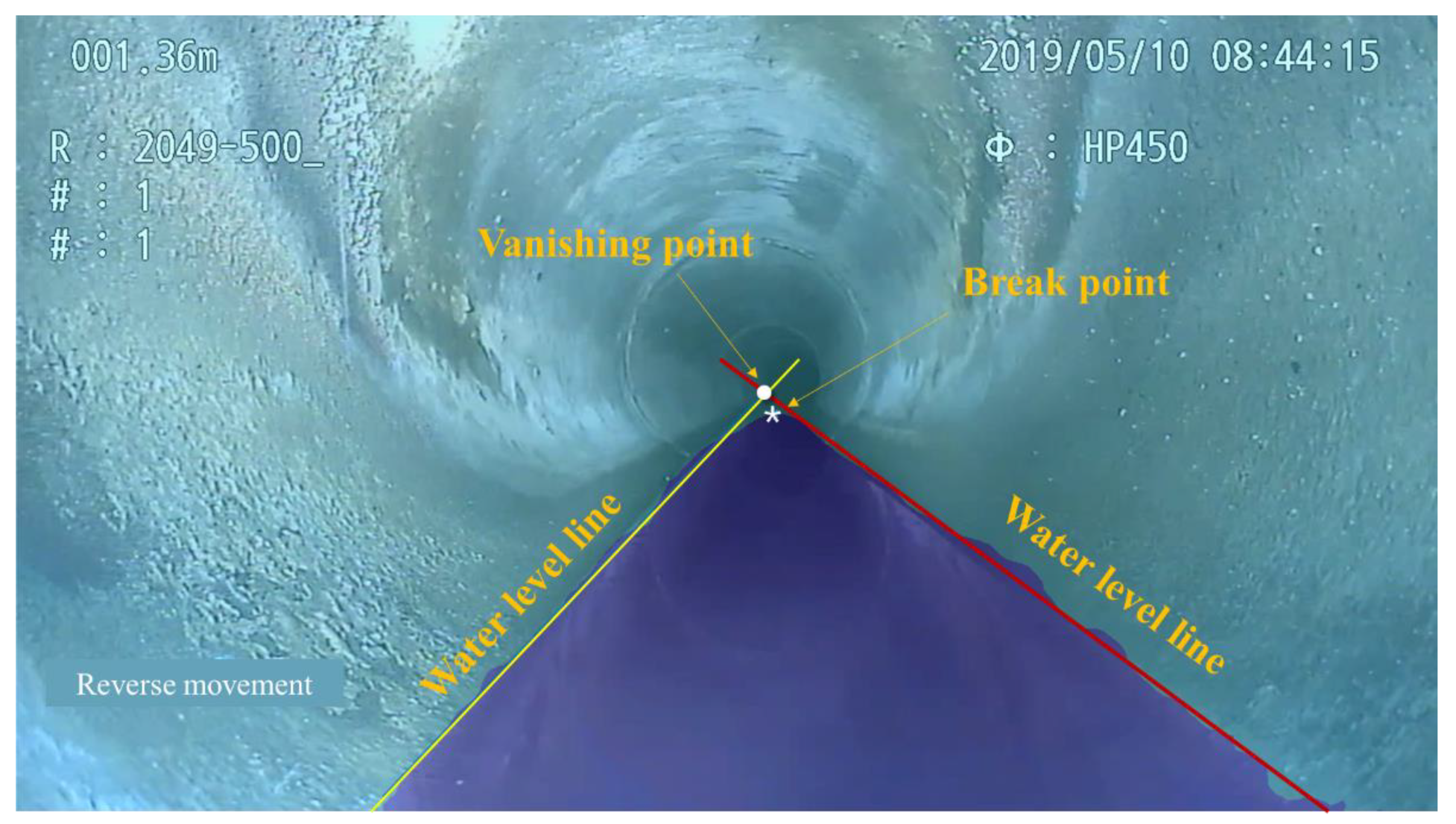
The CCTV footages taken from sewer pipe 2049-500 were divided into two areas through semantic segmentation using deep learning, and Figure 3 shows one frame among these results. The dark blue pixels below represent the sewer area, and the other light blue pixels represent the pipe area. The sewer area is shaped like a triangle, in which the bottom is wide and the top is pointed, and it can be seen that they gather to vanishing points according to the perspective.

The boundary line between the two areas is the line representing the water level. The area segmented by semantic segmentation is uneven. This is because the boundary between the water and pipe areas is ambiguous, and the concrete pipe is always wet and contaminated due to the constantly changing water level; thus, it is not easy to graphically distinguish between water and pipe areas. However, even under these conditions, the break point and least squares method were used to obtain the most interpretable water level lines. As a result, two water level lines and a vanishing point were obtained.

The water level lines and vanishing point are essential factors for calculating the water level. The water level was calculated by drawing an imaginary circle around the vanishing point, connecting the point where it meets the two lines (water level lines), and drawing a straight line that vertically passes through the vanishing point and these lines.

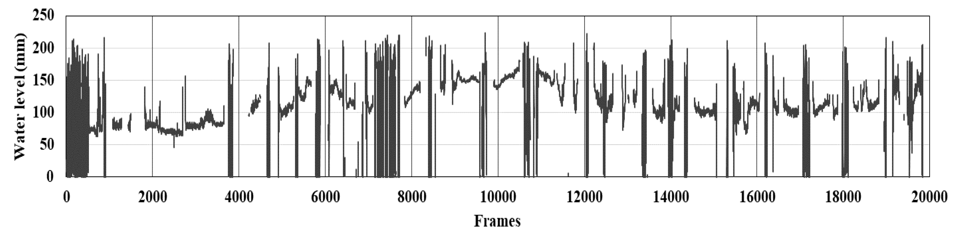
Figure 4 shows the water levels obtained from the entire CCTV footages, and the level ranged from 0 to 220 mm. These data have many errors, and three steps were applied to eliminate these errors.

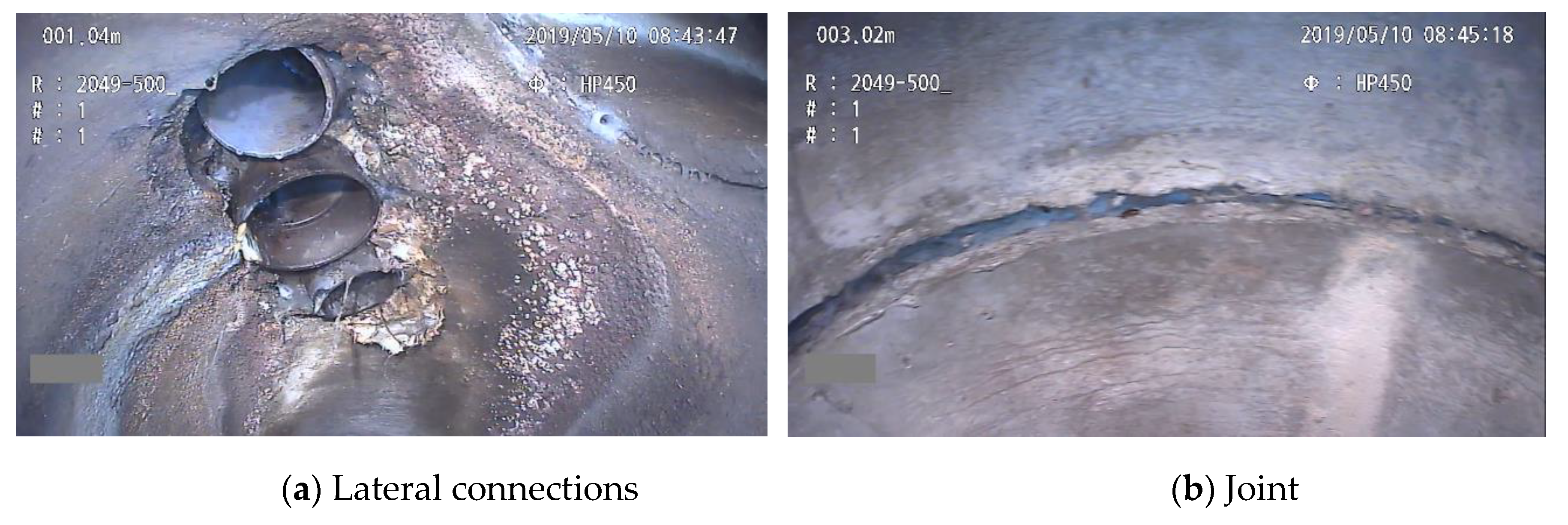
First, the data extracted from the frames containing connections or joints, images taken when CCTV camera entered the sewer pipe, and images taken from the retracting CCTV camera were deleted. CCTV video recording was performed by moving the camera straight along the sewer pipe, stopping the movement at the point where connections or joints were visible, and rotating the camera by 360°. The states of the corresponding conditions are shown in more detail in Figure 5a,b. Thus, it is reasonable that the number of sections where the extracted values severely fluctuate is the same as the number of connections and joints. There are 18 connections and 16 joints. Because one concrete pipe is 2.5 m long, and the length of the sewer pipe is 40.03 m, this number of joints is arithmetically appropriate. In addition, CCTV recording starts with the scene of entering a manhole with a screen showing information related to sewer pipes and video recording. The end of the video recording is a scene where CCTVs are retracted from the manhole on the other side. These two scenes are included in every CCTV footage. All four of these types of sections were deleted from the data, as shown in Figure 4.

Second, outliers were removed. When a box plot is drawn using the data obtained from the first step, outliners are revealed. These can be regarded as errors in image recognition by deep learning. The outliers are characterized by sporadic distribution without sections. Because the footage was taken at 30 frames per second, there cannot be any cases where the water level sharply increases or decreases in only one frame of 1/30 s. Thus, it is reasonable to regard such data as an error.

Third, a moving average was applied at 50 cm intervals to eliminate noise from the data. Deep learning recognizes images individually in all frames of a video, regardless of the causality of the preceding and following frames. Each frame can be changed by the movement of the camera, the flow of the sewer, insects, mice, and other various movements. Thus, the water level boundary recognized in each frame changes slightly, and the data fluctuate accordingly. Although fluctuations have value as raw data, they should be eliminated for convenience of analysis.

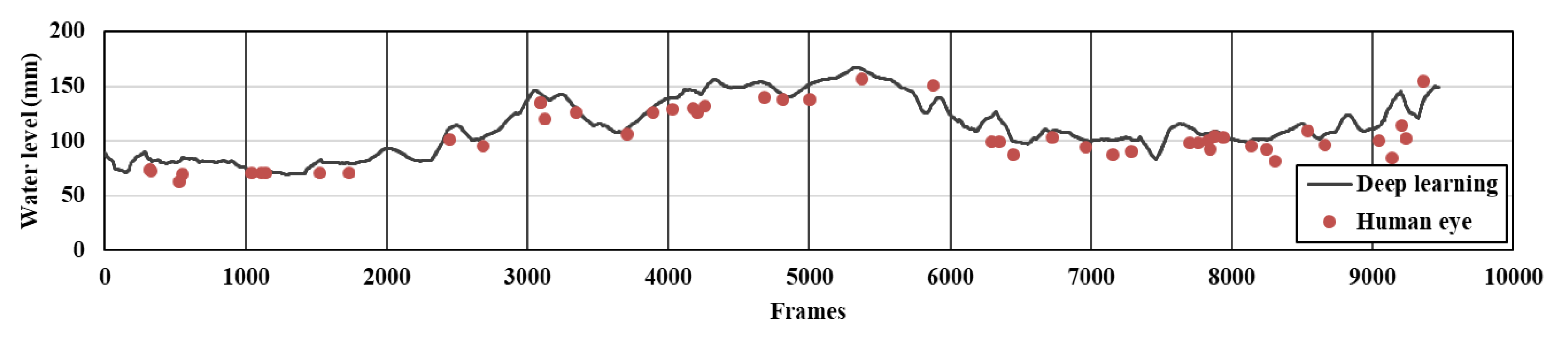
Figure 6 shows the data after modification by these three steps. There are 9467 frames, about half of the total 19,933 frames, corresponding to the water level. The overall trend is a mountain shape, in which the highest water level is in the middle of the sewer pipe (near 20 m), and the water level decreases toward both ends (0 m and 40.03 m). Therefore, this indicates that the sewer pipe is partially deflected. To check whether the result calculated by deep learning fits well, 50 frames were randomly extracted out of 9467 frames representing only the water level. The analyst marked the water level on the image using a straight line, and the calculated results were compared with the results obtained from deep learning. Figure 6 shows each value. Assuming that the value calculated directly by the analyst is a true value, the error rate of the value extracted by deep learning is 9.6%. This rate can be converted to an accuracy of 90.4%. This value is slightly lower than the case where the final accuracy was 98% when training was performed using the deep learning network. This can be attributed to various causes, such as the continuously changing CCTV screens, insufficient number of training data, and errors in human estimation of boundary lines.

It is considerably difficult to convert the water level calculated from CCTV footage into an elevation with distance and height information. Although the CCTV survey vehicle can record the mileage, and the video displays the mileage, the accuracy is not high enough to display the advanced distance per frame. To convert the water level to an elevation, the following assumption is required.

$$The first assumption:The running speed of the CCTV is constant.$$

Because the scenes containing connections, joints, and CCTV insertion and retraction were excluded from the CCTV footage in the process of modifying the data, the above assumption will not deviate significantly from the actual facts. Under the first assumption, if the number of frames is divided by the length of the sewer pipe (40.03 m), the driving speed is 1 m/234 frames. The distance can then be obtained by multiplying the frame number by the driving speed.

Unlike the water level, if the sewer pipe is not damaged, the slope of the elevation changes every 2.5 m, which is the production unit of the pipe. To apply this fact, the following two assumptions and one equation were applied:

$$The second assumption: J_i=d_{f=1} \left(i=1\right)$$

(1)

$$The third assumption:J_i=mean \mathrm{valueof}{d}_{f}between J_{i-1} and J_i \left(2\le i\le n+1\right)$$

(2)

$$J{E}_{relative, i}=J_1-J_i$$

(3)

where $J_i$ denotes the water level at the joint of the concrete pipe, $d_f$ denotes the water level at the frame of the CCTV, f denotes the frame number (1~9467), n denotes the pipe number (1~16), i denotes the joint number of sewer pipe (1~n + 1), and $J{E}_{relative, i}$ denotes the relative elevation at the joint.

The three equations described above were introduced to determine the relative elevation of the sewer pipe. Because pipes are connected by joints every 2.5 m, once the relative elevation of a joint is determined, the relative elevation of the sewer pipe can be determined accordingly. The water level of the first joint, the starting point of the sewer pipe, is based on the relative elevation, and the reference was assumed to be the water level ($d_1$) of the first frame (Equation (1)). Subsequently, the average of the water levels between the corresponding joint (i) and the previous joint (i−1) was assumed to be the corresponding water level ($J_i)$ of the joint (Equation (2)). This assumption is intended to cover all measurements. The relative elevation of the joint ($J{E}_{relative, i}$) is the amount of change compared to the reference (Equation (3)).

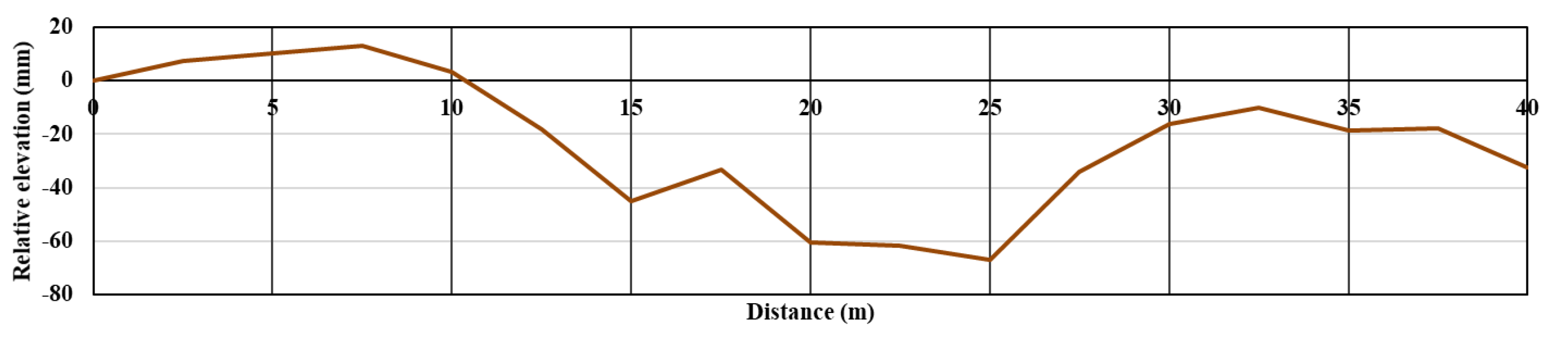
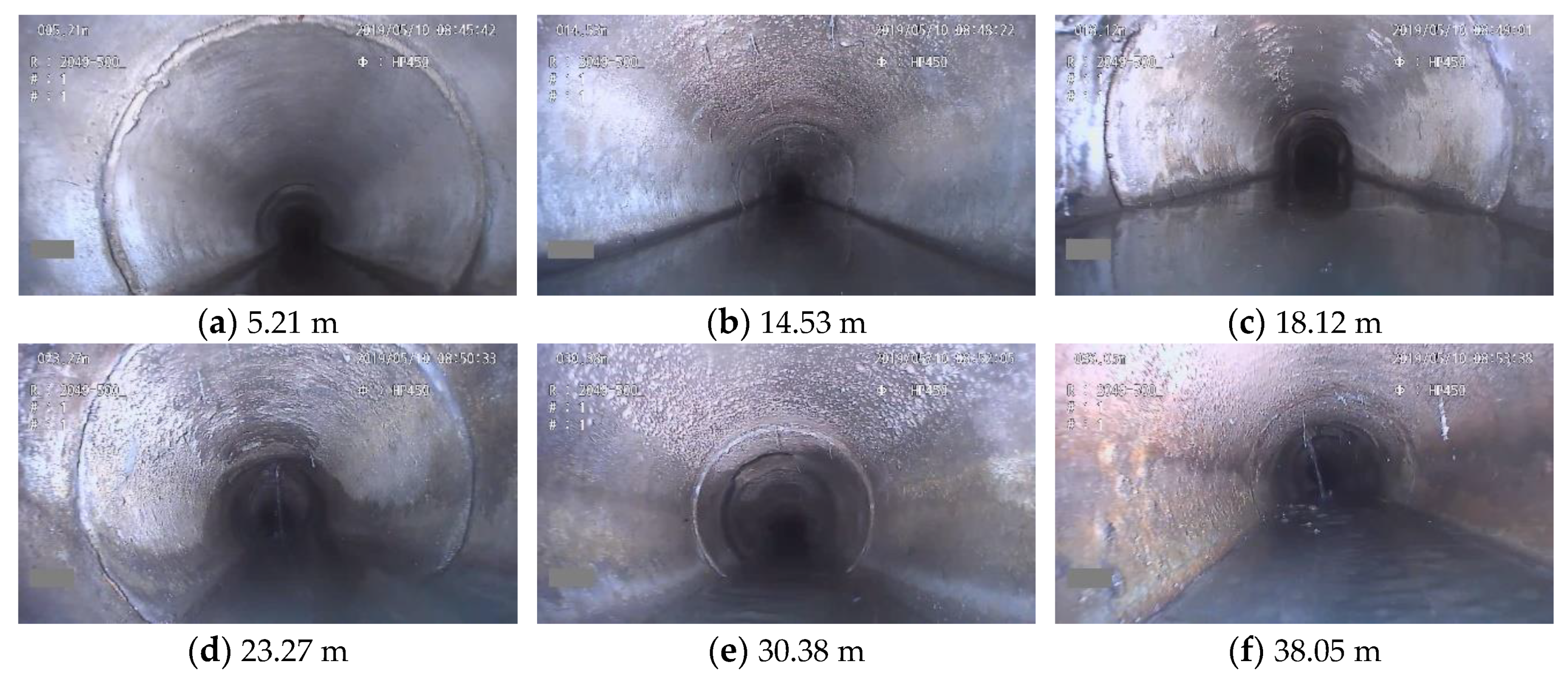
Figure 7 shows the relative elevation. From 0 to 10 m, the sewer pipe was slightly raised and then deflected. In particular, the deflection is the most significant between 15 and 25 m. In South Korea, the allowable construction error of sewer pipes is ±30 mm. At 25 m, the maximum deflection is 67 mm, which exceeds the allowable construction error by two times or more. This can also be intuitively checked in the CCTV footage. In Figure 8a, the water level is low, whereas the water level is high in Figure 8b,c. The water level becomes lower in Figure 8d,e and then higher again in Figure 8f.

The error rate of water levels calculated by the methodology proposed in this study is relatively lower than that of the results obtained using specific measuring instruments, such as lasers [5,6], ultrasonic devices [7,8], sonar [9], and CCTV with electronic tilt meter [10]. Factors that can affect the error of the results obtained using the measuring instruments are the error of the measuring instrument itself and errors due to the complex state of the sewer pipe. Among these errors, the error from the measuring instrument becomes considerably smaller due to careful verification and calibration during the production process. By contrast, the error from the complex state of the sewer pipe cannot be controlled.

There are many factors that can affect the error rate of measurements made using deep learning. The error rate is affected by the accuracy of the CNN, the amount of training data, the professionalism of the person creating the training data, the frame rate and resolution, and the conditions of the sewer pipe (e.g., corrosion, damage, fogging, rats, obstacles, and changes in brightness). The recent development of CNN has improved the accuracy of CNNs considerably and is continuously improving [22,23,24]. The amount of training data can be improved by changing the computer hardware conditions. However, analyst expertise or image quality is difficult to improve. This is because as the number of training images increases, the analyst’s fatigue increases and the precision decreases. It is difficult to change the image quality because each survey company provides only the quality prescribed by each local government. The complex condition of the sewer pipe is also an uncontrollable factor.

For the above reasons, it is difficult for a method using deep learning to have a smaller error rate than a method using a measuring instrument. Nevertheless, the methodology using deep learning has various advantages. This method does not need precise sensors, investigation time, and field work. Typically, CCTV footages are viewed only once immediately after an investigation and subsequently neglected, but in our study, the CCTV footages can be reused to extract quantitative data. In this respect, the utility value of CCTV footage becomes higher. Although the investigation report summarizing the existing CCTV footage includes the subsidence and steps of the pipe, it is difficult to use the data because the report lists various types of qualitative information. The methodology of this study produces data with excellent readability because it can graphically represent the slope of the pipe.

4. Conclusions

Local gradient changes in sewer pipes obstruct sewage flow, and they are one of the major causes of sedimentation, odor, and floods; therefore, such changes must be thoroughly investigated. In this study, the relative elevation inside a sewer pipe was determined after calculating the water level and identifying sewage from CCTV footage using deep learning. The training accuracy of deep learning was 98%, and the accuracy by comparison with random sample data was 92%. Owing to insufficient hardware, a recognition error was encountered because a relatively small number of images was employed for training. Statistical methods and increasing the number of training images by parallel processing using multiple GPUs can reduce the recognition error.

The relative elevation was determined using logical and mathematical methods; however, the results could not be verified using actual data. This is because a general method for the measurement of the elevation inside sewer pipes does not exist. A comparison study entailing various measurement methods will be helpful for verification.

The method proposed in this paper can be applied for prevention, cause analysis, and maintenance with regard to sewer odor, sedimentation, and flooding. Because all sewer pipes must undergo CCTV inspection at least once, the manager in charge will possess investigation videos. If the gradient of the sewer pipes in the target region is first investigated using CCTV survey footage, the sewer pipes can be effectively maintained because the sewer pipes that require special attention can be selected. In addition, the gradient change can be used to predict the amount of dredging and to increase the economic feasibility of dredging. Further, CCTV inspections based on these applications should be reconsidered as quantitative inspections.

References

- Yen, B.C.; Pansic, N. Surcharge of Sewer Systems; Water Resources Center Report Number 149; University of Ilinois: Urbana, IL, USA, 1980. [Google Scholar]
- Carr, R.W.; Esposito, C.; Walesh, S.G. Street-Surface Storage for Control of Combined Sewer Surcharge. J. Water Resour. Plan. Manag. 2001, 127, 162–167. [Google Scholar] [CrossRef]
- Fan, C.-Y.; Field, R.; Lai, F.-H. Sewer-Sediment Control: Overview of an Environmental Protection Agency Wet-Weather Flow Research Program. J. Hydraul. Eng. 2003, 129, 253–259. [Google Scholar] [CrossRef]
- Xu, Z.; Wu, J.; Li, H.; Chen, Y.; Xu, J.; Xiong, L.; Zhang, J. Characterizing heavy metals in combined sewer overflows and its influence on microbial diversity. Sci. Total Environ. 2018, 625, 1272–1282. [Google Scholar] [CrossRef] [PubMed]
- Duran, O.; Althoefer, K.; Seneviratne, L.D. Automated Pipe Defect Detection and Categorization Using Camera/Laser-Based Profiler and Artificial Neural Network. IEEE Trans. Autom. Sci. Eng. 2007, 4, 118–126. [Google Scholar] [CrossRef]
- Gunatilake, A.; Piyathilaka, L.; Kodagoda, S.; Barclay, S.; Vitanage, D. Real-Time 3D Profiling with RGB-D mapping in pipelines using stereo camera vision and structured IR laser ring. In Proceedings of the 14th IEEE Conference on Industrial Electronics and Applications (ICIEA), Xian, China, 19–21 June 2019; pp. 916–921. [Google Scholar]
- Gomez, F.; Althoefer, K.; Seneviratne, L. An ultrasonic profiling method for sewer inspection. In Proceedings of the IEEE International Conference on Robotics and Automation, New Orleans, LA, USA, 26 April–1 May 2004; 2004; Volume 5, pp. 4858–4863. [Google Scholar]
- Iyer, S.; Sinha, S.K.; Tittmann, B.R.; Pedrick, M.K. Ultrasonic signal processing methods for detection of defects in concrete pipes. Autom. Constr. 2012, 22, 135–148. [Google Scholar] [CrossRef]
- Lepot, M.; Pouzol, T.; Borruel, X.A.; Suner, D.; Bertrand-Krajewski, J.-L. Measurement of sewer sediments with acoustic technology: From laboratory to field experiments. Urban Water J. 2016, 14, 369–377. [Google Scholar] [CrossRef] [Green Version]
- Dirksen, J.; Pothof, I.; Langeveld, J.; Clemens, F. Slope profile measurement of sewer inverts. Autom. Constr. 2014, 37, 122–130. [Google Scholar] [CrossRef]
- LeCun, Y.; Bengio, Y.; Hinton, G. Deep learning. Nature 2015, 521, 436–444. [Google Scholar] [CrossRef] [PubMed]
- Myrans, J.; Kapelan, Z.; Everson, R. Automated Detection of Faults in Wastewater Pipes from CCTV Footage by Using Random Forests. Procedia Eng. 2016, 154, 36–41. [Google Scholar] [CrossRef] [Green Version]
- Kumar, S.S.; Abraham, D.M.; Jahanshahi, M.R.; Iseley, T.; Starr, J. Automated defect classification in sewer closed circuit television inspections using deep convolutional neural networks. Autom. Constr. 2018, 91, 273–283. [Google Scholar] [CrossRef]
- Haurum, J.B.; Moeslund, T.B. A Survey on Image-Based Automation of CCTV and SSET Sewer Inspections. Autom. Constr. 2020, 111, 103061. [Google Scholar] [CrossRef]
- Muste, M.; Hauet, A.; Fujita, I.; Legout, C.; Ho, H.-C. Capabilities of Large-scale Particle Image Velocimetry to characterize shallow free-surface flows. Adv. Water Resour. 2014, 70, 160–171. [Google Scholar] [CrossRef]
- Moy de Vitry, M.; Dicht, S.; Leitão, J.P. floodX: Urban flash flood experiments monitored with conventional and alternative sensors. Earth Syst. Sci. Data 2017, 9, 657–666. [Google Scholar] [CrossRef] [Green Version]
- Ji, H.W.; Yoo, S.S.; Lee, B.-J.; Koo, D.D.; Kang, J.-H. Measurement of Wastewater Discharge in Sewer Pipes Using Image Analysis. Water 2020, 12, 1771. [Google Scholar] [CrossRef]
- Mathworks. Available online: https://kr.mathworks.com/help/deeplearning/ref/resnet18.html#d120e51193 (accessed on 8 April 2020).
- Chen, L.-C.; Zhu, Y.; Papandreou, G.; Schroff, F.; Adam, H. Encoder-decoder with atrous separable convolution for semantic image segmentation. In Proceedings of the European Conference on Computer Vision (ECCV), Munich, Germany, 8–14 September 2018; pp. 801–818. [Google Scholar]
- Chee, J.; Li, P. Understanding and detecting convergence for stochastic gradient descent with momentum. arXiv 2020, arXiv:2008.12224. [Google Scholar]
- Mathworks. Available online: https://kr.mathworks.com/help/vision/ug/semantic-segmentation-using-deep-learning.html (accessed on 8 January 2021).
- Uchida, S.; Ide, S.; Iwana, B.K.; Zhu, A. A Further Step to Perfect Accuracy by Training CNN with Larger Data. In Proceedings of the 2016 15th International Conference on Frontiers in Handwriting Recognition (ICFHR), Shenzhen, China, 23–26 October 2016; pp. 405–410. [Google Scholar]
- Hofbauer, H.; Jalilian, E.; Uhl, A. Exploiting superior CNN-based iris segmentation for better recognition accuracy. Pattern Recognit. Lett. 2019, 120, 17–23. [Google Scholar] [CrossRef]
- Agrawal, A.; Mittal, N. Using CNN for facial expression recognition: A study of the effects of kernel size and number of filters on accuracy. Vis. Comput. 2020, 36, 405–412. [Google Scholar] [CrossRef]
Figure 1.
Process to determine water level from sanitary sewer CCTV inspection footage.
Figure 2.
Extraction of linear water level lines from edge of water area.
Figure 3.
Water level lines analyzed from CCTV footage by deep learning.
Figure 4.
Water level per frame of CCTV footage.
Figure 5.
Lateral connections (a) and joint (b) in CCTV footage.
Figure 6.
Comparison of the results of observations by the human eye and analysis by deep learning.
Figure 7.
The relative elevation inside the sewer pipe.
Figure 8.
Water level at location (a) 5.21 m, (b) 14.53 m, (c) 18.12 m, (d) 23.27 m, (e) 30.38 m, (f) 38.05 m in CCTV.
Publisher’s Note: MDPI stays neutral with regard to jurisdictional claims in published maps and institutional affiliations. |
© 2021 by the authors. Licensee MDPI, Basel, Switzerland. This article is an open access article distributed under the terms and conditions of the Creative Commons Attribution (CC BY) license (http://creativecommons.org/licenses/by/4.0/).
Share and Cite
MDPI and ACS Style
Ji, H.W.; Yoo, S.S.; Koo, D.D.; Kang, J.-H. Determination of Internal Elevation Fluctuation from CCTV Footage of Sanitary Sewers Using Deep Learning. Water 2021, 13, 503. https://doi.org/10.3390/w13040503
AMA Style
Ji HW, Yoo SS, Koo DD, Kang J-H. Determination of Internal Elevation Fluctuation from CCTV Footage of Sanitary Sewers Using Deep Learning. Water. 2021; 13(4):503. https://doi.org/10.3390/w13040503
Chicago/Turabian StyleJi, Hyon Wook, Sung Soo Yoo, Dan Daehyun Koo, and Jeong-Hee Kang. 2021. "Determination of Internal Elevation Fluctuation from CCTV Footage of Sanitary Sewers Using Deep Learning" Water 13, no. 4: 503. https://doi.org/10.3390/w13040503
Note that from the first issue of 2016, this journal uses article numbers instead of page numbers. See further details here.