
Numerical Evaluation of Fractional Vertical Soil Water Flow Equations


1
J. Amorocho Hydraulics Laboratory (JAHL), Department of Civil and Environmental Engineering, University of California, Davis, CA 95616, USA
2
Hydrologic Research Laboratory and JAHL, Department of Civil and Environmental Engineering, University of California, Davis, CA 95616, USA
*
Author to whom correspondence should be addressed.
Water 2021, 13(4), 511; https://doi.org/10.3390/w13040511
Submission received: 30 December 2020
/
Revised: 7 February 2021
/
Accepted: 12 February 2021
/
Published: 16 February 2021
(This article belongs to the Special Issue Modeling of Flow and Transport in Saturated and Unsaturated Porous Media)
Abstract
:Significant deviations from standard Boltzmann scaling, which corresponds to normal or Fickian diffusion, have been observed in the literature for water movement in porous media. However, as demonstrated by various researchers, the widely used conventional Richards equation cannot mimic anomalous diffusion and ignores the features of natural soils which are heterogeneous. Within this framework, governing equations of transient water flow in porous media in fractional time and multi-dimensional fractional soil space in anisotropic media were recently introduced by the authors by coupling Brooks–Corey constitutive relationships with the fractional continuity and motion equations. In this study, instead of utilizing Brooks–Corey relationships, empirical expressions, obtained by least square fits through hydraulic measurements, were utilized to show the suitability of the proposed fractional approach with other constitutive hydraulic relations in the literature. Next, a finite difference numerical method was proposed to solve the fractional governing equations. The applicability of the proposed fractional governing equations was investigated numerically in comparison to their conventional counterparts. In practice, cumulative infiltration values are observed to deviate from conventional infiltration approximation, or the wetting front through time may not be consistent with the traditional estimates of Richards equation. In such cases, fractional governing equations may be a better alternative for mimicking the physical process as they can capture sub-, super-, and normal-diffusive soil water flow processes during infiltration.
1. Introduction
Modeling soil water infiltration is realistically important for several applications in hydrology, meteorology, and environmental sciences since it connects surface and subsurface flow and transport processes. Based on Darcy’s law [1] and mass conservation, flow through unsaturated media is described by Richards equation [2] for the one-dimensional water flow in the vertical direction as,
Meanwhile, the soil hydraulic head (h) is related to the elevation head (z) and soil capillary pressure head (ψ) by = ψ(θ) + z, where is the volumetric water content, is the unsaturated hydraulic conductivity of the soil, is the hydraulic head, z is the distance in vertical direction, and t is the time. In the last century, several researchers contributed to the advancement of principles of the governing processes and predictive tools for infiltration dynamics in soils [3,4,5]. Hydraulic functions (e.g., [6,7,8,9]), which relate the hydraulic conductivity to the volumetric water content or to hydraulic head, are needed to solve Equation (1).
Although Richards equation has been extensively used to predict and model the transport of water, chemicals, and energy in soils, its usage is limited for heterogeneous soils [10]. Field measurements [11] demonstrated that soils in natural conditions can be highly heterogeneous and measurements of a transport property can be representative only in the immediate vicinity of a measured location. Conventional methods, including Richards approach, ignore the features of natural soils which undergo swelling and shrinking changes and cannot mimic anomalous diffusion, as explored and confirmed by various researchers [12,13]. There have been successful attempts to model the nonlinearity of layered soils [14,15], to treat preferential flow in shrinking soils by a dual-permeability approach [16,17], and to analyze the transient change of temperature and pressure between two adjacent homogeneous media for a variety of rock types [18]. However, the physical theory linking flow in soils and macropores (i.e., preferential flow, nonequilibrium flow, or dual porosity flow) is inadequate, and observational methods are not sufficient to obtain scale-dependent parameterization in field and hillslope scales [19].
Anomalous or non-Fickian transport of solutes in porous media was reported for several field and laboratory applications (e.g., [20,21,22,23,24]), with Boltzmann scaling (x/tq where q = 0.5) corresponding to normal, or Fickian diffusion being modeled by the conventional Richards equation. Significant deviations from standard Boltzmann scaling have been observed in the literature for horizontal and vertical water movement. For horizontal water flow, Pachepsky et al. [25] reported that the mean values of the time exponent q, 〈q〉 for Columbia silt loam and Hesperia sandy loam in Nielsen et al. [26] were 0.344 ≤ 〈q〉 ≤ 0.480, while those for Salkum silty clay loam in Rawlins and Gardner [27] were 0.430 ≤ 〈q〉 ≤ 0.479, and those for Salkum silty clay loam in Ferguson and Gardner [28] were 0.452 ≤ 〈q〉 ≤ 0.465. For vertical soil water flow, Voller [29] reported that the initial advance of the wetting front of some cases in a set of 28 field infiltration measurements taken by Logsdon [30] exhibited anomalous super-diffusion behavior. Nielsen et al. [26] explained the mechanism of anomalous (i.e., non-Fickian) diffusion in unsaturated flows by “jerky movements” of the wetting front due to the heterogeneous nature of the size, shape, composition, and arrangement of soil particles that lead to continuous changes in the shape of the air–water interface. Non-Newtonian behavior of the water due to impurities, large pressure gradients at the water–air interface, partially open pores, and the fractal nature of the soils are also considered to be the causes of the non-Fickian behavior of transport in the soil medium [10,31,32].
Water movement in porous building materials, which deviates from the Fickian diffusion mechanism, was reported by Kündtz and Lavallee [33] and El Abd and Milczarek [34]. Consistent with the earlier literature, both studies confirmed that the time exponent q varies with the nature of the disordered porous media with fractal geometry. Kündtz and Lavallee [33] assumed a modified Fick’s equation (i.e., taking volumetric moisture flow as a function of the moisture gradient of power n, where n is a real number) and proposed a nonlinear diffusion equation for partially saturated materials. El Abd and Milczarek [34] followed the approach of Kündtz and Lavallee [33] and proposed that the diffusivity coefficient must depend not only on the water content but also on time, as was previously proposed [35,36].
Within this framework, several researchers attempted to improve soil water infiltration modeling by utilizing fractional differentiation in order to model non-Fickian or anomalous diffusion in soil water flow. For other possible approaches to model such anomalous behavior, see Zhang et al. [24] and the references therein. A fractional differential model for seepage flow in porous media was proposed and its approximate analytical solution by the variational iteration method was constructed by He [37]. In order to model horizontal soil water flow, Pachepsky et al. [25] utilized a fractional time derivative with an order equal to or less than one, while Gerolymatou et al. [38] proposed a fractional integral form for the Richards equation in fractional time, and Sun et al. [39] replaced the integer-order time derivative of the water content by a fractal derivative by utilizing the concept of fractal ruler in time. With respect to vertical soil water flow, Voller [29] proposed a fractional Green–Ampt infiltration model and expressed the spatial derivative in the hydraulic flux as a Caputo fractional derivative of the head. Extending the work by Su [13], who studied vertical infiltration into swelling soils by the fractional time derivative, Su [40] presented mass–time and space–time fractional partial differential equations (fPDEs) of water movement for swelling–shrinking soils and non-swelling soils and showed that the fractional infiltration models better fit the field data of Talsma and van der Lelij [41] using a fractional cumulative infiltration model. Su [40] utilized power functions in the fPDEs for diffusivity and hydraulic conductivity which depend on the moisture content.
Recently, starting from Caputo fractional derivative approximation of a function, Kavvas et al. [42] derived the dimensionally consistent equations of continuity and motion for transient soil water flow and soil water flux to obtain the governing equation for transient soil water flow in fractional multidimensional space and fractional time. Closed forms of the governing equations were then obtained from Brooks–Corey relationships [6]. The classical diffusivity expression in the conventional Richards equation for soil water flow depends only on the soil water content, i.e., D = D(). Kavvas et al. [42]’s theoretical development not only considers the time-dependent diffusivity that was previously reported [33,35,36] as D = E() tm, but can also address diffusivity that may change in space (see Equation (52) in [42]). Due to fractional powers of the space and time derivatives, the proposed governing equations can capture nonlocal effects in time (time history of the flow) and nonlocal effects in space (long-range dependence in the porous media). In other words, the proposed fractional soil water flow equations have the capacity to account for the effect of the initial conditions on the soil water flow for long periods, and for the effect of the boundary conditions on the flow for long distances by changing the fractional powers [42]. The nonlocality in time can be physically due to mass transfer between relatively immobile and mobile phases, and interaction between segregated regions of high and low permeability [40,43,44]. The nonlocality in space, on other hand, can be physically due to high variation and long spatial autocorrelation of permeability, as is the case of preferential flow paths [40,45,46]. Furthermore, the time and space fractional derivative powers in fractional water movement account for the non-Fickian flow processes, in which the time fractional derivative power corresponds to long time correlations leading to sub-diffusive or slow processes, but the space fractional derivative power corresponds to long space correlations leading to super-diffusive processes [40,47]. Lastly, when the powers of fractional time and space derivatives go to unity, the governing equation simplifies to its conventional counterparts.
Although Kavvas et al. [42] provided the theoretical derivation of the new generalized governing equations of soil water flow and flux in fractional differential derivative framework, it lacks a methodology to solve the proposed fractional governing equations and an application that explores the significance of fractional powers and coefficients in the governing equations. Within this framework, the purposes of this study are threefold. Firstly, instead of utilizing Brooks–Corey relationships, empirical expressions which were obtained from least square fits through hydraulic measurements for soil water movements [48] were utilized in this study to show the general applicability of the proposed fractional governing equations of soil water flow and soil water flux with not only Brooks–Corey relationships but also other constitutive hydraulic relations in the literature. Secondly, a numerical solution methodology for the fractional vertical soil water flow was presented to solve the developed theory in Kavvas et al. [42]. Lastly, the capabilities of the proposed fractional differentiation approach for vertical soil water flow were investigated in comparison to conventional governing equations. Sub-, super-, and normal-diffusive soil water flow cases were explored numerically within the framework of Zaslavsky [47]’s definition of the transport exponent.
2. Methodology
2.1. Fractional Derivatives
Unlike integer order derivatives, the fractional derivative of a function depends on its values over an interval [xa, x] and can therefore capture nonlocal effects. The fractional derivative of a function g(x) for order 0 in Caputo sense is defined as follows [49]:
where is the gamma function. When the power β goes to unity, the Caputo derivative of g(x) becomes the same as the integer order derivative [50]. Conventional governing equations are based on integer order derivatives that are local. On other hand, local derivatives within an interval [xa, x] contribute to the fractional derivative for that interval with varying weights as defined in Equation (2), which makes the fractional derivative nonlocal. Since the Caputo fractional derivative in Equation (2) can be written for both space and time derivatives, nonlocality both in space and time can be obtained by changing the fractional power β. A detailed review of the concepts of fractional calculus is provided in [50,51]. The fractional differentiation in the Caputo framework was chosen in the derivation of the governing equations of the fractional soil water flow and flux [42] since physically interpretable initial and boundary conditions can be utilized in the Caputo framework, unlike various other fractional differentiation frameworks.
2.2. Fractional Soil Water Flow
A generalized approach that can handle both Fickian and non-Fickian behavior through a fractional differentiation framework for soil water infiltration modeling is practical and quite conceivable. The spatial variability of heterogeneous soils can be quantitatively characterized by fractal dimensions, which can capture the geometric complexity of soils and characterize them with a few numbers [10]. Although the full dynamical processes occurring in soils may not be described by the so-called fractal dimension, the fractal geometry has great potential to be utilized in various ways in soil science [52]. Fractional powers ( and in Equation (3) below), in a similar manner to the role of fractals in geometry, can be utilized in a fractional governing equation for the infiltration process, by which one can represent nonlocal effects in time and space.
With this motivation, Kavvas et al. [42] developed the equations of continuity and motion for transient soil water flow and soil water flux and combined them to deduce the governing equation for transient soil water flow in multidimensional fractional soil space and fractional time as:
where the fractional soil water flux is:
Here, 0 < α, β1, β2, β3 < 1 are the fractional orders or powers of space and time fractional derivatives, = is the spatial location, and Ki is the hydraulic conductivity in the i-spatial direction (i = 1, 2, 3). When fractional orders of space and time derivatives go to unity, the above fractional governing equation for soil water flow becomes the conventional Richards equation.
For convenience in the rest of the manuscript, we have replaced x3 with z for the vertical dimension, β3 with β as the fractional power for space, with q as the fractional soil water flux, and K3 with K as the hydraulic conductivity in the vertical direction. Then, the fractional governing equation for the vertical direction is simplified to:
and
Kavvas et al. [42] then obtained the closed form of the above equations by introducing the Brooks–Corey relationships [6]. In this study, instead of Brooks–Corey relationships, empirical expressions, obtained by least square fits through hydraulic measurements for Yolo light clay and sand (as provided in Haverkamp et al. [48]) were used. Further details are provided in the Numerical Applications section.
2.3. Numerical Solution
Following Murio [53], the first-order approximation of Caputo’s fractional time derivative of a function f can be approximated by
where the time interval [0, T] is divided into N subintervals of equal increment dt = T/N using the nodes tn where n = 0, 1, 2, …, N, and , , .
Dividing the space interval [0, a] into M subintervals of equal increments dz = a/M using the nodes zj where j = 0, 1, 2, …, M, the Caputo fractional space derivative at a > 0 can be approximated in second order by [54]
where 0 < β ≤1 is the fractional order of the space derivative and is the first-order derivative at zj. Utilizing Equation (5), the fractional soil water flow equation given by Equation (5) can be written as
where and . The space fractional derivatives and can be calculated by Equation (8).
3. Numerical Applications
Haverkamp et al. [48] compared an implicit numerical solution of Richards equation with Philip’s quasi-analytical solution [5,55] for soil water movements in Yolo light clay and sand (Figure 4 and Table 3 in [48]). Here, we utilize the same infiltration problems to estimate the water front through time to be able to compare the solutions of the conventional Richards approach with the numerical solution of the case β = α = 1 of the proposed fractional vertical soil water flow equations. In other words, Table 3 in Haverkamp et al. [48] is actually used to provide a baseline for the numerical solution of the case β = α= 1 of the proposed fractional vertical soil water flow equations. After verifying that the proposed fractional model works for the standard Richards equation by setting β = α = 1, fractional powers are altered to investigate the corresponding anomalous diffusion behavior within the framework of Zaslavsky [47]’s definition of the transport exponent, which depends on the powers of the space and time fractional derivatives of the governing diffusion equation.
The first example problem for infiltration through Yolo light clay is an experiment that was used by Philip [5,55], for which the hydraulic conductivity and water content relationships are:
Ks = 4.428.10−2 cm/h, and where the subscript s refers to saturation and r refers to residual. The initial and boundary conditions for the first problem are:
For the second problem, i.e., the infiltration through sand, the hydraulic conductivity and water content relationships, as provided in Haverkamp et al. [48] are:
where Ks = 34 cm/h, . These relationships are based on experimental measurements [56,57]. The initial and boundary conditions for the second problem are:
4. Results and Discussion
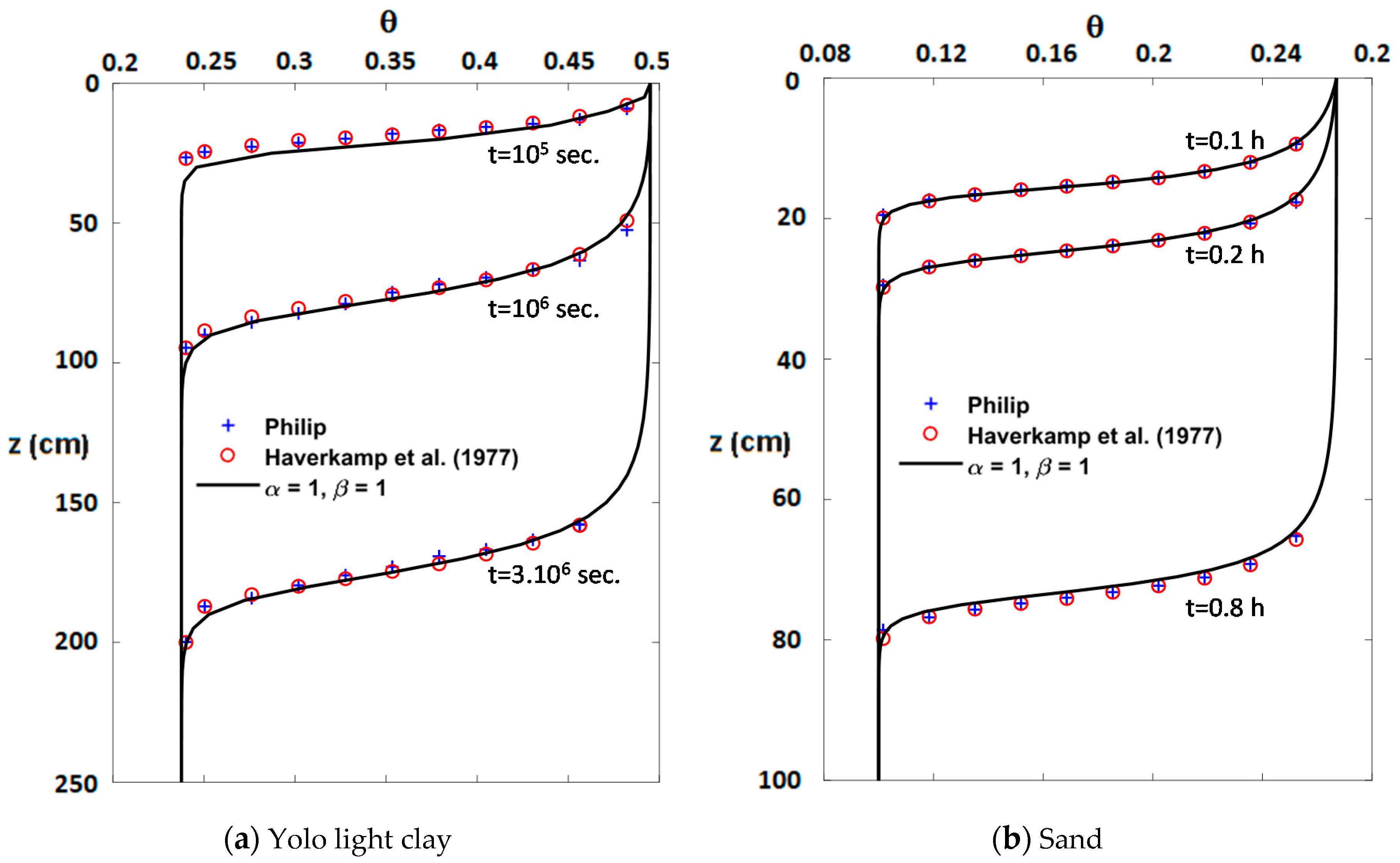
Utilizing the numerical examples for infiltration through the Yolo light clay and sand [48], one of the purposes of this study was to explore the capabilities of fractional governing equations to simulate vertical soil water flow compared to their integer order conventional counterparts. When the fractional powers of space and time derivatives of the fractional vertical soil water equation become one, the solution should converge to the conventional Richards equation (Equation (1)). Figure 1 depicts the comparison between the water content profiles of the Philip solution [5,55], h-implicit solution [48], and the proposed fractional governing equations when space and time fractional derivative powers are unity, i.e., β = α = 1. The fractional approach, within this framework, when solved numerically by the scheme in Equation (9), produces results that are quite similar to the conventional solutions of Richards equation for the infiltration problems through Yolo light clay and sand. When compared with the Philip solution, the correlation coefficient and Nash–Sutcliffe efficiency values were 0.9996 and 0.9991 for Yolo light clay, and 0.9998, and 0.9995 for sand. When compared with the h-implicit solution [48], the correlation coefficient and Nash–Sutcliffe efficiency values were 0.9998 and 0.9993 for Yolo light clay, and 0.9999 and 0.9995 for sand, respectively.
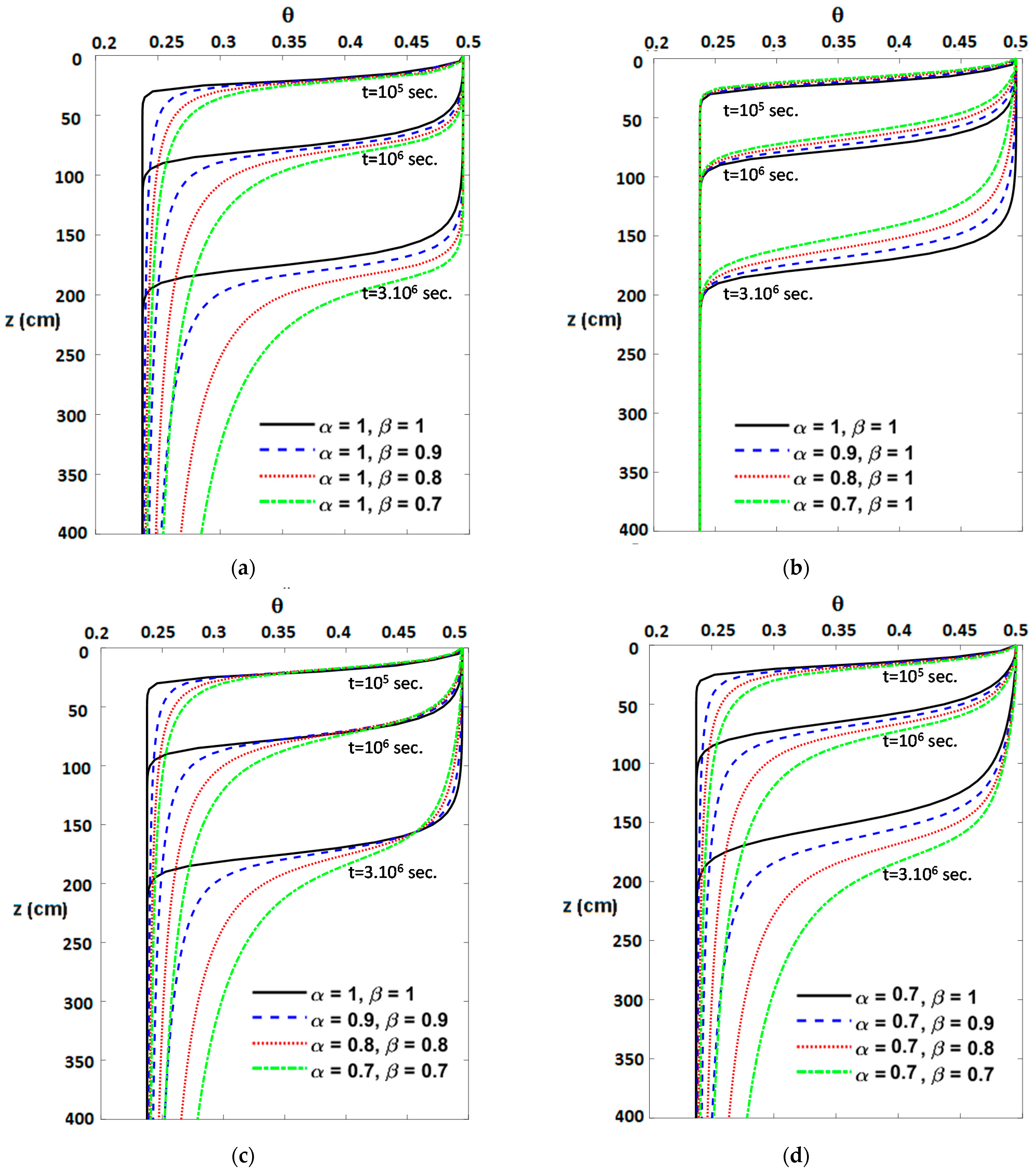
We now explore the effects of the space and time fractional derivative powers on the vertical water movement as proposed in Equation (5) above. Comparisons among water content profiles when space and time fractional derivative powers are fractional are depicted in Figure 2 for Yolo light clay and in Figure 3 for sand. The transport exponent µ quantifies the competing time and space fractional derivative powers or the competing sub- and super-diffusivity [47]: µ < 1 is for sub-diffusion, µ = 1 for classical or normal diffusion, and µ > 1 is for super-diffusion. The transport exponent is defined as µ = 2β/α where β is the power of time derivative and α is the total power of the space derivative for the diffusive term [47]. To be consistent with our notations, β in [47] is replaced with α, and α in [47] is replaced with 2β so that the transport exponent becomes µ = 2α/2β = α/β in our notation.
For the case when the power of the time fractional derivative is one (α = 1), the wetting front moves down faster as the power of the space fractional derivative decreases from 1 (β < 1 in Figure 2a for Yolo light clay and Figure 3a for sand). The wetting front for the lower moisture content moves down even faster than that of the higher moisture content. In light of the above transport exponent definition, the cases (when β < 1) in Figure 2a for Yolo light clay and Figure 3a for sand correspond to super-diffusion since the transport exponent, µ, is greater than 1 (µ > 1) since α = 1, β < 1. This finding is consistent with [40], who stated that the space fractional derivatives cause super-diffusion, mainly by the flow processes in the media with higher velocity flow paths of long spatial correlation.
For the case of when the power of the space fractional derivative is one (β = 1), the wetting front slows down as the power of the time fractional derivative decreases from 1 (Figure 2b for Yolo light clay and Figure 3b for sand). The wetting front for the higher moisture content slows down even more than that of the lower moisture content. These cases (when α < 1) in Figure 2b for Yolo light clay and Figure 3b for sand correspond to sub-diffusion since the transport exponent, µ, is less than 1 (µ < 1) since α < 1, β = 1. This finding is also consistent with [40], who stated that the time fractional derivatives result in sub-diffusion, mainly by partitioning of water parcels on sticky porous surfaces.
When the powers of time and space fractional derivatives are equal and decrease from one, the effects of time and space fractional powers, as discussed above, are superimposed (Figure 2c for Yolo light clay and Figure 3c for sand). The transport exponent µ = α/β becomes one, showing overall normal diffusion in theory. However, as the time and space fractional powers decrease from 1, the movement of the wetting front for the higher moisture content slows down and that of the wetting front for the lower moisture content moves down faster.
For the case when the power of the time fractional derivative is 0.7 (α = 0.7), the wetting front moves down faster as the power of the space fractional derivative decreases from 1 (β < 1 in Figure 2d for Yolo light clay). The wetting front for the lower moisture content moves down even faster than that of the higher moisture content. On other hand, for the case when the power of the space fractional derivative is 0.7 (β = 0.7), the wetting front slows down as the power of the time fractional derivative decreases from 1 (Figure 3d for sand). The wetting front for the higher moisture content slows down even more than that of the lower moisture content.
After investigating water content profiles through time, we now examine the performances of cumulative infiltration approximations by a conventional approach and a fractional approach. As opposed to Philip [58]’s approximate description of the cumulative infiltration for conventional vertical infiltration into rigid media
where A is the final infiltration rate and S is the sorptivity. On other hand, Su [40] conjectured a cumulative infiltration model for water movement in soils as
where 0 < α ≤2 is the order of the time fractional derivative, and 0 < λ ≤ 2 is the order of the mass (for swelling soils) or the space (for non-swelling soils) fractional derivative of the diffusion term. When Equation (23) was fitted to the field data of cumulative infiltration versus time as reported by Figure 1 in [41], parameters α, λ, A, and S were determined by Su [40] as α = 0.3445, λ = 1.9523, A = 1.30 mm/day, and S = 48.64 . Compared to Equation (22) for the conventional vertical infiltration (see Figure 1b in [13]), Equation (23) provides a considerably better fit to the field data of [41], confirming the superior performance of fractional cumulative infiltration models. The transport exponent for field data of [41], µ = 0.353, corresponds to sub-diffusion [40].
Lastly, the cumulative infiltration values were calculated using the fractional model for eight different time instances for Yolo light clay (t = 105, 2.5 × 10⁵, 5 × 10⁵, 106, 1.5 × 10⁶, 2 × 10⁶, 2.5 × 10⁶, 3 × 10⁶ s) and for sand (t = 0.1, 0.2, 0.3, …, 0.8 h) when α = β = 0.9, 0.8, 0.7. The conventional and fractional cumulative infiltration approximations in Equations (22) and (23) require the estimation of two parameters, the final infiltration rate A, and the sorptivity S. Using the cumulative infiltration estimates of the first and last time instances, A and S can be calculated for the two models and the performance of both models can be evaluated based on the cumulative infiltration approximations for the remaining six time instances. Table 1 and Table 2 provide the percent difference between the approximated and simulated cumulative infiltration values (I(simulated) − I(approximated))/I(simulated) for Yolo light clay and sand, respectively. Since the parameters A and S are estimated based on the first and last time instances, approximations at these times are same as the simulated values, i.e., the percent difference values are 0. The percent difference values are less than 2.5% for Yolo light clay and 0.5% for sand when the fractional cumulative infiltration approximation (Equation (23)) is used. The percent difference values are less than 8% for Yolo light clay and 3% for sand when the conventional cumulative infiltration approximation (Equation (22)) is used. Hence, the fractional cumulative infiltration approximation (Equation (23)) performed better than the conventional cumulative infiltration model (Equation (22)) when the powers of time and space fractional derivatives are fractional.
In practice, as in the case of [41], the observed cumulative infiltration values can deviate from the conventional cumulative infiltration approximation (Equation (22)), or the wetting front through time may not be consistent with the traditional estimates of Richards equation. In such cases the fractional governing equations may be a better alternative to mimic the physical process, and the fractional approximation (Equation (23)) can be a better alternative for the estimation of the cumulative infiltration.
5. Conclusions
In this study, empirical expressions obtained by least square fits through hydraulic measurements for soil water movements (Haverkamp et al. [48]) were utilized to show the general applicability of the proposed fractional governing equations of soil water flow and soil water flux [42] with not only Brooks–Corey relationships but also other constitutive hydraulic relations in the literature. A numerical solution methodology for the fractional vertical soil water flow was presented to solve the fractional governing equations of vertical soil water flow. Finally, the modeling capabilities of the fractional governing equations of vertical soil water flow were investigated numerically for infiltration problems through Yolo light clay and sand. It was demonstrated for both flow media that when the powers of space and time fractional derivatives are one, the fractional approach provides solutions that are same as the conventional Richards equation approach. Furthermore, the numerical investigation demonstrated that:
- (a)
- When the power of the time fractional derivative is one, the wetting front moves down faster (super-diffusive behavior) as the power of the space fractional derivative decreases from 1. The wetting front for the lower moisture content moves down even faster than that corresponding to the higher moisture content.
- (b)
- When the power of the space fractional derivative is one, the wetting front slows down (sub-diffusive behavior) as the power of the time fractional derivative decreases from one. Additionally, the wetting front for the higher moisture content slows down even more than that of the lower moisture content.
- (c)
- When the powers of time and space fractional derivatives are equal, the effects of time and space fractional powers are superimposed. The transport exponent µ becomes one, showing overall normal diffusion in theory. However, as the time and space fractional powers decrease from one to zero, the wetting front for the higher moisture content slows down (sub-diffusive behavior) while the wetting front for the lower moisture content moves down faster (super-diffusive behavior). To our knowledge, this combined sub- and super-diffusive behavior with a resultant normal diffusion has been reported for the first time and should be investigated further in future studies.
- (d)
- The fractional cumulative infiltration approximation (Equation (23)) performs better than the conventional cumulative infiltration model (Equation (22)) when the powers of time and space fractional derivatives are fractional.
To conclude, as in the case of [41], the observed cumulative infiltration values in practice can deviate from the conventional cumulative infiltration approximation. In such cases where the wetting front through time may not be consistent with the traditional estimates of the Richards equation, the fractional governing equations may be a better alternative to mimic the physical process of vertical soil water flow, and the fractional approximation can be a better alternative for the estimation of the cumulative infiltration. Although the numerical study herein provides helpful insights to the capabilities of the proposed fractional approach in terms of the fractional powers of the space and time derivatives, further research is needed to combine experimental and field studies with the proposed theory of fractional soil water movement.
Author Contributions
Formal analysis, numerical simulations, visualization, writing—original draft: A.E.; Conceptualization, methodology, review and editing: M.L.K., A.E. All authors have read and agreed to the published version of the manuscript.
Funding
This research received no external funding.
Institutional Review Board Statement
Not applicable.
Informed Consent Statement
Not applicable.
Data Availability Statement
The data presented in this study are available on request from the corresponding author.
Conflicts of Interest
The authors declare no conflict of interest.
References
- Darcy, H. Les Fontaines Publiques de la Ville de Dijon; Dalmont: Paris, France, 1856. [Google Scholar]
- Richards, L.A. Capillary conduction of liquids through porous medium. Physics 1931, 1, 318–333. [Google Scholar] [CrossRef]
- Green, W.H.; Ampt, G.A. Studies on soil physics: I. Flow of air and water through soils. J. Agr. Sci. 1911, 4, 1–24. [Google Scholar]
- Horton, R.E. An approach towards a physical interpretation of infiltration capacity. Soil Sci. Soc. Am. Proc. 1940, 5, 399–417. [Google Scholar] [CrossRef]
- Philip, J.R. The theory of infiltration: 1. The infiltration equation and its solution. Soil Sci. 1957, 83, 345–357. [Google Scholar] [CrossRef]
- Brooks, R.H.; Corey, A.T. Hydraulic Properties of Porous Media; Colorado State University: Fort Collins, CO, USA, 1964; Volume 3, p. 27. [Google Scholar]
- Gardner, W.R. Field measurement of soil water diffusivity. Proc. Soil Sci. Soc. Am. 1970, 34, 832–833. [Google Scholar] [CrossRef]
- Mualem, Y. A new model for predicting the hydraulic conductivity of unsaturated porous media. Water Resour. Res. 1976, 12, 513–522. [Google Scholar] [CrossRef] [Green Version]
- Van Genuchten, M.T. A closed-form equation for predicting the hydraulic conductivity of unsaturated soils. Soil Sci. Soc. Am. J. 1980, 44, 892–898. [Google Scholar] [CrossRef] [Green Version]
- Bartoli, F.; Dutartre, P.; Gomendy, V.; Niquet, S.; Dubuit, M.; Vivier, H. Fractals and Soil Structure. In Fractals in Soil Science; Baveye, P., Parlange, J.-Y., Stewart, B.A., Eds.; CRC Press: Boca Raton, FL, USA, 1998. [Google Scholar]
- Nielsen, D.R.; Biggar, J.W.; Erh, K.T. Spatial variability of field measured soil-water properties. Hilgardia 1973, 42, 215–260. [Google Scholar] [CrossRef] [Green Version]
- Hilfer, R. Applications of Fractional Calculus in Physics; World Scientific Publishing Company: Singapore, 2000. [Google Scholar]
- Su, N. Theory of infiltration: Infiltration into swelling soils in a material coordinate. J. Hydrol. 2010, 395, 103–108. [Google Scholar] [CrossRef]
- Berardi, M.; Difonzo, F.; Vurro, M.; Lopez, L. The 1D Richards’ equation in two layered soils: A Filippov approach to treat discontinuities. Adv. Water Resour. 2018, 115, 264–272. [Google Scholar] [CrossRef]
- Suk, H.; Park, E. Numerical solution of the Kirchhoff-transformed Richards equation for simulating variably saturated flow in heterogeneous layered porous media. J. Hydrol. 2019, 579. [Google Scholar] [CrossRef]
- Coppola, A.; Gerke, H.H.; Comegna, A.; Basile, A.; Comegna, V. Dual-permeability model for flow in shrinking soil with dominant horizontal deformation. Water Resour. Res. 2012, 48, W08527. [Google Scholar] [CrossRef]
- Gerke, H.H.; van Genuchten, M.T. A dual porosity model for simulating the preferential movement of water and solute in structured porous media. Water Resour. Res. 1993, 29, 305–319. [Google Scholar] [CrossRef]
- Salusti, E.; Kanivetsky, R.; Droghei, R.; Garra, R. On the propagation of nonlinear transients of temperature and pore pressure in a thin porous boundary layer between two rocks. J. Hydrol. 2019, 576, 620–627. [Google Scholar] [CrossRef]
- Beven, K.; Germann, P. Macropores and water flow in soils revisited. Water Resour. Res. 2013, 49, 3071–3092. [Google Scholar] [CrossRef] [Green Version]
- Sudicky, E.A.; Cherry, J.A.; Frind, E.O. Migration of contaminants in groundwater at a landfill: A case study. 4. A natural-gradient dispersion test. J. Hydrol. 1983, 63, 81–108. [Google Scholar] [CrossRef]
- Sidle, C.; Nilson, B.; Hansen, M.; Fredericia, J. Spatially varying hydraulic and solute transport characteristics of a fractured till determined by field tracer tests, Funen, Denmark. Water Resour. Res. 1998, 34, 2515–2527. [Google Scholar] [CrossRef]
- Silliman, S.E.; Simpson, E.S. Laboratory evidence of the scale effect in dispersion of solutes in porous media. Water Resour. Res. 1987, 23, 1667–1673. [Google Scholar] [CrossRef]
- Levy, M.; Berkowitz, B. Measurement and analysis of non-Fickian dispersion in heterogeneous porous media. J. Contam. Hydrol. 2003, 64, 203–226. [Google Scholar] [CrossRef]
- Zhang, Y.; Benson, D.A.; Reeves, D.M. Time and space nonlocalities underlying fractional-derivative models: Distinction and literature review of field applications. Adv. Water Resour. 2009, 32, 561–581. [Google Scholar] [CrossRef]
- Pachepsky, Y.; Timlin, D.; Rawls, W. Generalized Richards’ equation to simulate water transport in unsaturated soils. J. Hydrol. 2003, 272, 3–13. [Google Scholar] [CrossRef]
- Nielsen, D.R.; Biggar, J.W.; Davidson, J.M. Experimental consideration of diffusion analysis in unsaturated flow problem. Soil Sci. Soc. Am. Proc. 1962, 26, 107–111. [Google Scholar] [CrossRef]
- Rawlins, S.L.; Gardner, W.H. A test of the validity of the diffusion equation for unsaturated flow of soil water. Soil Sci. Soc. Amer. 1963, 27, 507–511. [Google Scholar] [CrossRef]
- Ferguson, H.; Gardner, W.H. Diffusion theory applied to water flow data obtained using gamma ray absorption. Soil Sci. Soc. Amer. Proc. 1963, 27, 243–246. [Google Scholar] [CrossRef]
- Voller, V.R. On a fractional derivative form of the Green–Ampt infiltration model. Adv. Water Resour. 2011, 34, 257–262. [Google Scholar] [CrossRef]
- Logsdon, S.D. Transient variations in the infiltration rate during measurement with tension infiltrometers. Soil Sci. 1999, 162, 233–241. [Google Scholar] [CrossRef]
- Dullien, F.A.L. Porous Media: Fluid Transport and Pore Structure; Academic Press: New York, NY, USA, 1979. [Google Scholar]
- Warrick, A.W. Soil Water Dynamics; Oxford University Press: Oxford, UK, 2003. [Google Scholar]
- Kündtz, M.; Lavallee, P. Experimental evidence and theoretical analysis of anomalous diffusion during water infiltration in porous building materials. J. Phys. D Appl. Phys. 2001, 34, 2547–2554. [Google Scholar] [CrossRef]
- El-Abd, A.E.-G.; Milczarek, J.J. Neutron radiography study of water absorption in porous building materials: Anomalous diffusion analysis. J. Phys. D Appl. Phys. 2004, 37, 2305–2313. [Google Scholar] [CrossRef]
- Guerrini, I.A.; Swartzendruber, D. Soil water diffusivity as explicitly dependent on both time and water content. Soil Sci. Soc. Am. J. 1992, 56, 335–340. [Google Scholar] [CrossRef]
- Lockington, L.A.; Parlange, J.-Y. Anomalous water absorption in porous materials. J. Phys. D Appl. Phys. 2003, 36, 760–767. [Google Scholar] [CrossRef]
- He, J.-H. Approximate analytical solution for seepage flow with fractional derivatives in porous media. Comput. Methods Appl. Mech. Eng. 1998, 167, 57–68. [Google Scholar] [CrossRef]
- Gerolymatou, E.; Vardoulakis, I.; Hilfer, R. Modelling infiltration by means of a nonlinear fractional diffusion model. J. Phys. D Appl. Phys. 2006, 39, 4104–4110. [Google Scholar] [CrossRef] [Green Version]
- Sun, H.-G.; Meerschaert, M.M.; Zhang, Y.; Zhu, J.; Chen, W. A fractal Richards’ equation to capture the non-Boltzmann scaling of water transport in unsaturated media. Adv. Water Resour. 2013, 52, 292–295. [Google Scholar] [CrossRef] [Green Version]
- Su, N. Mass-time and space-time fractional partial differential equations of water movement in soils: Theoretical framework and application to infiltration. J. Hydrol. 2014, 519, 1792–1803. [Google Scholar] [CrossRef]
- Talsma, T.; van der Lelij, A. Infiltration and water movement in an in situ swelling soil during prolonged ponding. Aust. J. Soil Res. 1976, 14, 337–349. [Google Scholar] [CrossRef]
- Kavvas, M.L.; Tu, T.; Ercan, A.; Polsinelli, J. Governing equations of transient soil water flow and soil water flux in multi-dimensional fractional anisotropic media and fractional time. Hydrol. Earth Syst. Sci. 2017, 21, 1547–1557. [Google Scholar] [CrossRef] [Green Version]
- Haggerty, R.; McKenna, S.A.; Meigs, L.C. On the late-time behavior of tracer test breakthrough curves. Water Resour. Res. 2000, 36, 3467–3479. [Google Scholar] [CrossRef] [Green Version]
- Berkowitz, B.; Scher, H. Theory of anomalous chemical transport in random fracture network. Phys. Rev. E 1998, 57, 5858–5869. [Google Scholar] [CrossRef] [Green Version]
- Herrick, M.G.; Benson, D.A.; Meerschaert, M.M.; McCall, K.R. Hydraulic conductivity, velocity, and the order of the fractional dispersion derivative in a highly heterogeneous system. Water Resour. Res. 2002, 38, 1227. [Google Scholar] [CrossRef]
- Zhang, Y.; Benson, D.A.; Meerschaert, M.M.; LaBolle, E.M. Space-fractional advection–dispersion equations with variable parameters: Diverse formulas, numerical solutions, and application to the MADE-site data. Water Resour. Res. 2007, 43, W05439. [Google Scholar] [CrossRef] [Green Version]
- Zaslavsky, G.M. Chaos, fractional kinetics, and anomalous transport. Phys. Rep. 2002, 37, 461–580. [Google Scholar] [CrossRef]
- Haverkamp, R.; Vauclin, M.; Touma, J.; Wierenga, P.J.; Vachaud, G. A comparison of numerical simulation models for one-dimensional infiltration. Soil Sci. Soc. Am. J. 1977, 41, 285–294. [Google Scholar] [CrossRef]
- Caputo, M. Linear models of dissipation whose Q is almost frequency independent, part II. Geophys. J. Int. 1967, 13, 529–539. [Google Scholar] [CrossRef]
- Podlubny, I. Fractional Differential Equations; Academic Press: New York, NY, USA, 1999. [Google Scholar]
- Oldham, K.B.; Spanier, J. The Fractional Calculus; Academic Press: New York, NY, USA, 1974. [Google Scholar]
- Baveye, P.; Parlange, J.-Y.; Stewart, B.A. Fractals in Soil Science; CRC Press: Boca Raton, FL, USA, 1998. [Google Scholar]
- Murio, D.A. Implicit finite difference approximation for time fractional diffusion equations. Comput. Math. Appl. 2008, 56, 1138–1145. [Google Scholar] [CrossRef]
- Odibat, Z.M. Computational algorithms for computing the fractional derivatives of functions. Math. Comput. Simul. 2009, 79, 2013–2020. [Google Scholar] [CrossRef]
- Philip, J.R. The theory of infiltration: 2. The profile of infinity. Soil Sci. 1957, 83, 435–448. [Google Scholar] [CrossRef]
- Watson, K.K. An instantaneous profile method for determining the hydraulic conductivity of unsaturated porous materials. Water Resour. Res. 1966, 2, 709–715. [Google Scholar] [CrossRef]
- Vachaud, G.; Thony, J.L. Hysteresis during infiltration and redistribution in a soil column at different initial water contents. Water Resour. Res. 1971, 7, 111–127. [Google Scholar] [CrossRef]
- Philip, J.R. Theory of infiltration. Adv. Hydrosci. 1969, 5, 215–296. [Google Scholar]
Figure 1.
Comparisons between water content profiles of the Philip solution, h-implicit solution [48], and the proposed fractional governing equations when space and time fractional derivative powers for (a) Yolo light clay and (b) Sand. Both the Philip and h-implicit solutions are provided in Table 3 in [48].

Figure 2.
Comparison among water content profiles for Yolo light clay when space and time fractional derivative powers are (a) 1 and , 0.9, 0.8, 0.7; (, 0.9, 0.8, 0.7; (c), 0.9, 0.8, 0.7; (d) 0.7 and , 0.9, 0.8, 0.7.
Figure 2.
Comparison among water content profiles for Yolo light clay when space and time fractional derivative powers are (a) 1 and , 0.9, 0.8, 0.7; (, 0.9, 0.8, 0.7; (c), 0.9, 0.8, 0.7; (d) 0.7 and , 0.9, 0.8, 0.7.

Figure 3.
Comparison between water content profiles for sand when space and time fractional derivative powers are (a) 1 and , 0.9, 0.8, 0.7, 0.9, 0.8, 0.7; (c), 0.9, 0.8, 0.7; (d), 0.9, 0.8, 0.7.
Figure 3.
Comparison between water content profiles for sand when space and time fractional derivative powers are (a) 1 and , 0.9, 0.8, 0.7, 0.9, 0.8, 0.7; (c), 0.9, 0.8, 0.7; (d), 0.9, 0.8, 0.7.


Table 1.
Comparison of simulated cumulative infiltration with two approximations: The fractional model (Equation (23)), and the conventional model (Equation (22)) by Philip [58] for Yolo light clay.
Table 1.
Comparison of simulated cumulative infiltration with two approximations: The fractional model (Equation (23)), and the conventional model (Equation (22)) by Philip [58] for Yolo light clay.
| Percent Difference (Equation (23)) | Percent Difference (Equation (22)) | ||||||
|---|---|---|---|---|---|---|---|
| t (s) | t (day) | 0.9 | 0.8 | 0.7 | 0.9 | 0.8 | 0.7 |
| 100,000 | 1.16 | 0.000% | 0.000% | 0.000% | 0.000% | 0.000% | 0.000% |
| 250,000 | 2.89 | 0.468% | 0.373% | −0.394% | −5.874% | −5.468% | −5.262% |
| 500,000 | 5.79 | 0.237% | 0.581% | 1.013% | −7.983% | −7.089% | −5.376% |
| 1,000,000 | 11.57 | −0.013% | 1.610% | 2.283% | −7.107% | −5.071% | −3.366% |
| 1,500,000 | 17.36 | 0.004% | 1.735% | 1.791% | −5.101% | −3.138% | −2.408% |
| 2,000,000 | 23.15 | 0.033% | 1.104% | 1.370% | −3.172% | −2.009% | −1.332% |
| 2,500,000 | 28.94 | 0.070% | 0.508% | 0.803% | −1.435% | −0.976% | −0.494% |
| 3,000,000 | 34.72 | 0.000% | 0.000% | 0.000% | 0.000% | 0.000% | 0.000% |
Table 2.
Comparison of simulated cumulative infiltration with two approximations: The fractional model (Equation (23)), and the conventional model (Equation (22)) by Philip [58] for sand.
Table 2.
Comparison of simulated cumulative infiltration with two approximations: The fractional model (Equation (23)), and the conventional model (Equation (22)) by Philip [58] for sand.
| Percent Difference (Equation (23)) | Percent Difference (Equation (22)) | |||||
|---|---|---|---|---|---|---|
| t (h) | 0.9 | 0.8 | 0.7 | 0.9 | 0.8 | 0.7 |
| 0.1 | 0.000% | 0.000% | 0.000% | 0.000% | 0.000% | 0.000% |
| 0.2 | −0.400% | 0.121% | −0.297% | −2.610% | −2.006% | −2.111% |
| 0.3 | −0.435% | 0.148% | −0.396% | −2.834% | −2.194% | −2.416% |
| 0.4 | −0.203% | 0.249% | −0.206% | −2.270% | −1.794% | −1.981% |
| 0.5 | −0.068% | 0.125% | −0.148% | −1.647% | −1.453% | −1.525% |
| 0.6 | −0.037% | −0.175% | −0.162% | −1.084% | −1.232% | −1.087% |
| 0.7 | −0.008% | −0.234% | −0.115% | −0.522% | −0.757% | −0.575% |
| 0.8 | 0.000% | 0.000% | 0.000% | 0.000% | 0.000% | 0.000% |
Publisher’s Note: MDPI stays neutral with regard to jurisdictional claims in published maps and institutional affiliations. |
© 2021 by the authors. Licensee MDPI, Basel, Switzerland. This article is an open access article distributed under the terms and conditions of the Creative Commons Attribution (CC BY) license (http://creativecommons.org/licenses/by/4.0/).
Share and Cite
MDPI and ACS Style
Ercan, A.; Kavvas, M.L. Numerical Evaluation of Fractional Vertical Soil Water Flow Equations. Water 2021, 13, 511. https://doi.org/10.3390/w13040511
AMA Style
Ercan A, Kavvas ML. Numerical Evaluation of Fractional Vertical Soil Water Flow Equations. Water. 2021; 13(4):511. https://doi.org/10.3390/w13040511
Chicago/Turabian StyleErcan, Ali, and M. Levent Kavvas. 2021. "Numerical Evaluation of Fractional Vertical Soil Water Flow Equations" Water 13, no. 4: 511. https://doi.org/10.3390/w13040511
Note that from the first issue of 2016, this journal uses article numbers instead of page numbers. See further details here.