Assessing Chlorophyll a Spatiotemporal Patterns Combining In Situ Continuous Fluorometry Measurements and Landsat 8/OLI Data across the Barataria Basin (Louisiana, USA)

Abstract

The acquisition of reliable and accurate data to assess environmental changes over large spatial scales is one of the main limitations to determine the impact of eutrophication, and the effectiveness of management strategies in coastal systems. Here, we used a continuous in situ Chl-a fluorometry sensor and L8/OLI satellite data to develop an algorithm and map Chl-a spatial distribution to assess the impact of freshwater diversions and associated high nutrient loading rates in the Barataria Basin (BB) complex, a coastal system in the northern Gulf of Mexico. We collected water quality samples at 24 sampling stations and high-frequency continuous fluorometry in situ [Chl-a] data along a ~87 km transect from 2019–2020. Field [Chl-a] values were highly correlated (r = 0.86; p < 0.0001) with continuous in situ [Chl-a] fluorometry values. These continuous in situ [Chl-a] values were significantly related to a surface reflectance ratio ([B1 + B4]/B3) estimated using L8/OLI data (exponential model; R² = 0.46; RMSE = 4.8, p < 0.0001). The statistical model replicated [Chl-a] spatial patterns across the BB complex. This work shows the utility of high-frequency continuous Chl-a fluorometry sampling coupled with L8/OLI image analysis to increase the frequency and number of field data sets to assess water quality conditions at large spatial scales in highly dynamic deltaic regions.

1. Introduction

Estuaries are coastal ecosystems characterized by a high biological diversity and productivity across latitudes [1]. However, despite their ecological and economic importance, estuaries are increasingly altered by anthropogenic impacts that modify biogeochemical cycling and ecosystem services (e.g., fisheries, water quality; [2,3]). Currently, coastal eutrophication is a pervasive environmental problem that alters the complex functional and structural properties of estuaries across fertility and salinity gradients [4,5,6,7,8]. Understanding the relationship between eutrophication processes and estuarine functional attributes has become a priority as managers seek to mitigate and regulate eutrophication at different spatiotemporal scales.

One of the major limitations to improving water quality and mitigating negative impacts caused by coastal eutrophication is the lack of data and information to evaluate the frequency, duration, and spatial extent of nutrient enrichment impacts on ecosystem primary productivity. Although eutrophication assessment initiatives have been developed since the 1950’s in the USA, the lack of extensive and intensive spatiotemporal data coverage still limits the development of more comprehensive regional evaluations, particularly the long term impacts of nitrogen (N) and phosphorous (P) loadings [9]. Since the 1990’s the National Estuarine Eutrophication Assessment (NEEA; 1999, 2007) has determined, for instance, the scale, scope and origin of nutrient enrichment conditions in 144 estuaries in the conterminous U.S. [9,10]. Yet, in coastal regions there are still data gaps to fully understand the environmental effects of increasing eutrophication mainly due to urban and industrial development that have critically altered the hydrology and geomorphology of watershed systems in a changing climate [11,12,13].

Nutrient enrichment in estuarine systems triggers a progression of eutrophic responses [14,15]. The most apparent is the significant increase of Chlorophyll a concentration (hereafter Chl-a) and macroalgal blooms [14] that are directly correlated to high N and P loading rates into estuarine and coastal waters [16,17]. Because phytoplankton rapidly responds to nutrient availability (i.e., hourly/daily), Chl-a is considered a good proxy to determine the eutrophic state of estuarine waters [18]. Indeed, since Chl-a is the main source of phytoplankton’s in vivo fluorescence [19,20], this biophysical property has promoted the development of remote sensing tools that use optical sensors to indirectly evaluate in situ fluorometry and determine phytoplankton productivity and biomass at large spatial scales (i.e., hundreds of km²; [18,19,21]). Yet, assessing rapid changes in Chl-a at large spatial scales in both coastal and inland waters using remote sensing instruments is still a challenge.

One of the major issues in the spatial extrapolation and interpolation of field data is separating the contribution of in situ water column optical properties from the actual optical signals (i.e., in vivo fluorescence/absorbance) of phytoplankton cells (i.e., “Case 2” waters; [22,23]). Although in vivo fluorescence is well correlated to Chl-a concentrations, there are interfering compounds or processes that can significantly affect this relationship. It is known, for instance, that taxonomic composition, physiological/morphological mechanisms (e.g., light, trophic status, nutrient stress), and turbidity are factors affecting the accuracy of Chl-a estimates via remote sensing [24,25,26,27]. Furthermore, in shallow systems, bottom reflectance often interferes with the phytoplankton signal in the water column [28].

To reduce this uncertainty when assessing Chl-a values, spatiotemporal trends of in situ fluorescence or absorbance measurements are needed to identify the relative contribution of other environmental factors to explain the total variance when converting fluorometric values to Chl-a values. To date, Chl-a datasets available for the calibration and evaluation of Chl-a/fluorometric models are limited in frequency and in spatial extend [21]. In this study, we use high-resolution, spatially explicit in situ data to increase the accuracy of Chl-a mapping in the Barataria Basin (USA; hereafter BB complex). The study site is a dynamic trophic estuarine system where optical water column properties are largely determined by the Mississippi River discharge fluctuations throughout the year [29,30].

We compiled data sets from a continuous water quality sampling system (i.e., SWAMMP-R) and contemporaneous Landsat 8/OLI (L8/OLI) images to develop a Chl-a detection algorithm for time series of L8/OLI images. Given the OLI sensor configurations of Landsat 8 (i.e., Operational Land Imager) that collect data from nine shortwave bands, it is possible to pair and calibrate image data with continuous field in situ Chl-a fluorometry values collected in estuarine and coastal waters at the pixel level. Specifically, the objectives of this study were to (1) evaluate continuous in situ Chl-a fluorometry values acquired over a large spatial scale that were coupled with L8/OLI images acquisition to increase the accuracy of statistical models linking continuous fluorometric-based Chl-a values to L8/OLI surface reflectance and (2) use these models to discern Chl-a spatial variability along salinity gradients in the BB complex. We particularly focus on locations impacted by controlled freshwater diversions aiming to enhance sediment inputs for wetland restoration and can introduce nutrients that may promote algae blooms including toxic cyanobacteria species [31,32,33,34]. Further, freshwater diversions could potentially trigger complex responses over extended coastal areas. These include the effects of increasing flooding duration, changes in relative elevation and accretion rates in wetlands, and reduction in salinity due to freshwater inputs [31,32,33,34,35]. Because controlled freshwater diversions can also increase N and P loading rates, we also determine the potential impact on phytoplankton biomass at variable spatial scales defined by differences in fertility gradients [35,36]. We hypothesize that the impact of freshwater water diversions on the BB complex plankton biomass reflected in Chl-a values can be accurately and efficiently assessed using a combination of calibrated statistical models and spatially intensive sampling using the continuous flow-thru SWAMMP-R (Spatially explicit WAter Monitoring system to inform Management Priorities and Risks) multiprobe. Understanding the spatiotemporal patterns and the interactions among hydrology and primary production at a landscape level in the BB complex will provide critical data and information to determine and quantify the effects of freshwater diversions on this complex estuarine system undergoing extensive wetland and hydrological restoration since the 1990′s [33]. This assessment is urgently needed to gauge both the present BB complex eutrophication magnitude and future changes as freshwater diversions are implemented in brackish and saline regions within the next 10 years [32,35,37,38].

2. Materials and Methods

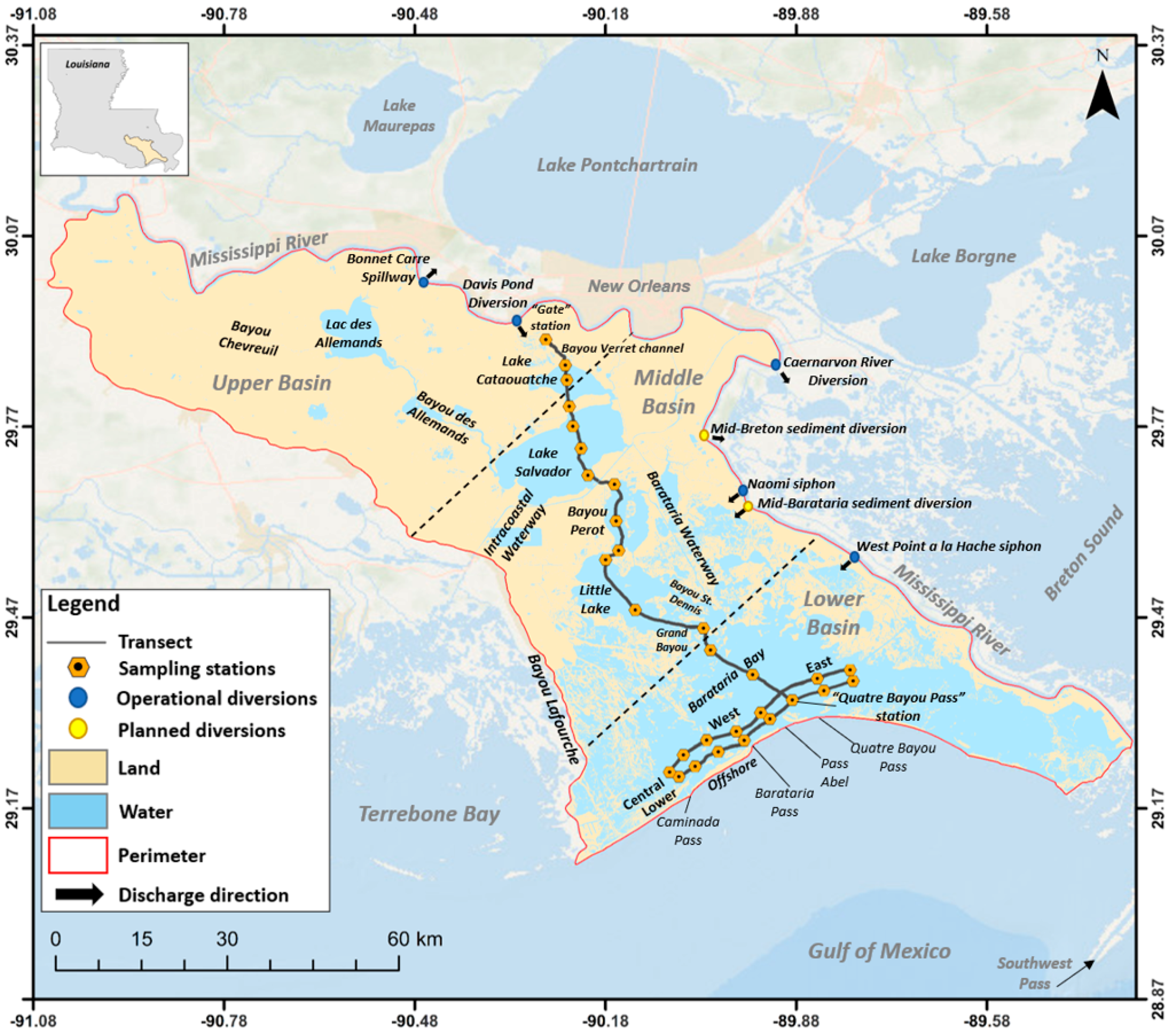
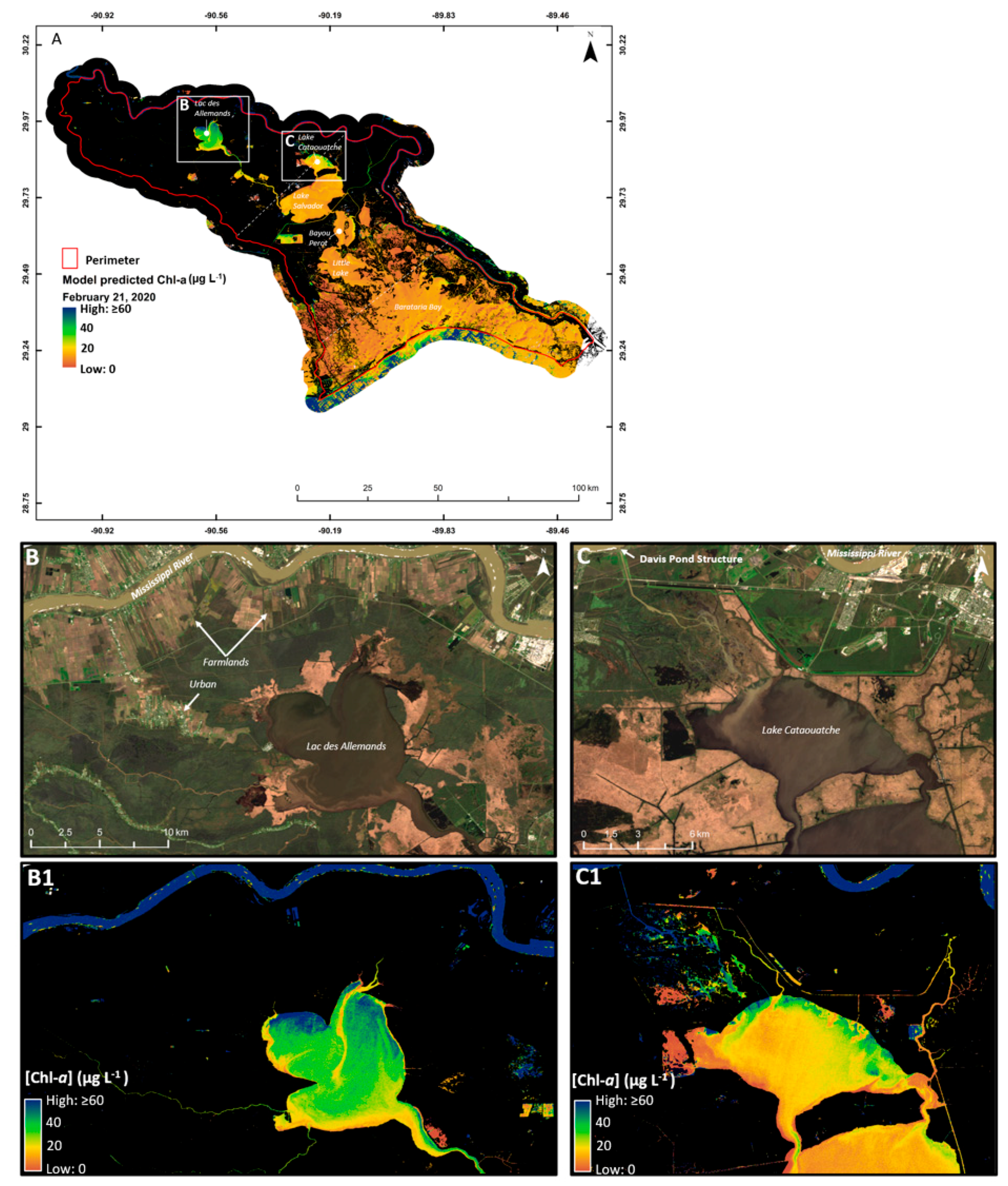
2.1. Area Description

The Barataria Basin (i.e., BB complex) is considered one of the most productive estuarine systems in the northern Gulf of Mexico (nGOM) [39,40,41,42]. It is located between the west bank of the Mississippi River (MR) and Bayou Lafourche in southeastern Louisiana, USA (range: latitude, 29°5′ to 30°8′ N; longitude, 89°21′ to 91°3′ W) (Figure 1). This area is part of the Mississippi River Delta Plain (MRDP) and characterized by high levels of primary production due to high nutrient loading rates from the MR and agriculture/urban areas in the upper basin. The MR is the longest river system in North America (7854 km; including the Missouri river) and it ranks sixth and seventh globally in terms of water (610 km³ yr⁻¹) and sediment (210 Mt yr⁻¹) discharge [43,44,45]. The BB complex has a total area of approximately 6600 km² with the highest elevations ranging from ~4–5 m along natural levees and the lowest slightly above sea level in wetland areas [46]. Vegetation communities are well-defined in the basin from north to south with cypress-tupelo swamp defined by Taxodium distichum and Nyssa aquatica and freshwater marsh characterized by Panicum hemitomon, Eleocharis spp., and Sagittaria lancifolia at the upper basin; an intermediate-brackish marsh dominated by Spartina patens and Distichilis spicata at the middle basin; and saltwater marsh habitat dominated by Spartina alterniflora at the lower basin [46,47,48]. The total land area in the BB complex comprises agriculture fields (765 km²), urban areas (430 km²) and extensive wetlands (3587 km²) [49]. The major water bodies in the BB complex include Lac des Allemands and Lake Cataouatche at the upper basin; Lake Salvador, Bayou Perot, and Little Lake in the middle basin; and Barataria Bay proper at the lower basin (Figure 1). Mean water depth in this region ranges from 1.5–2.0 m [50,51]. The water residence time is variable among water bodies: 50–70 days in the middle of Lac des Allemands; 100–120 days in Lake Cataouatche; 100 days in Lake Salvador; 8–15 days in Bayou Perot; 10–30 days in Little Lake; and 1–4 days in Barataria Bay [52,53].

Water quality properties across the BB complex are determined by daily and seasonal drivers including tidal fluctuations, atmospheric factors controlling meteorological events (i.e., cold fronts, storms, and tropical cyclones), river discharge and anthropogenic activities. The BB complex is a micro tidal system with mixed diurnal and semi-diurnal tides. The daily tidal amplitude average is 0.32 m at the coast and 0.03 m at the upper basin; this tidal range is significantly influenced by wind during the winter season when cold fronts occur at 3–7 days duration while tidal oscillation is the main driver during the summer season [49,54,55]. Cold fronts in coastal Louisiana are characterized by a strong wind shear, an abrupt drop in atmospheric pressure, and a fast reduction in air temperature [56]. Although cold fronts are not as severe as tropical cyclones, wind direction/velocity control water levels and circulation, sediment transport (e.g., fluxes, wetland accretion/erosion, sediment resuspension), and the exchange of organic matter and nutrients between the BB complex and the GOM [38,56]. Because of the BB complex location in subtropical latitudes, maritime tropical air masses maintain persistent warm and humid conditions along coastal Louisiana [38,57]. Thus, mean annual temperature ranges from 19 °C (January) to 32 °C (July) (mean: 20 °C) while the minimum average ranges from 7 °C (January) to 22 °C (July) [38,57].

The main freshwater inputs into the basin are rainwater, surface runoff from surrounding areas, the Gulf Intracoastal Waterway, and the Davis Pond Freshwater Diversion (DPFD) located in the upper basin with a maximum operational discharge of 250 m³ s⁻¹ [53,54]. Although levees along the Mississippi River have reduced the hydrological connectivity between the river and the adjacent wetlands, freshwater discharge from the Southwest Pass is advected from the mouth into the estuary through tidal inlets. This exchange promotes inputs of freshwater (c.a., ~200 m³ s⁻¹; [58]), salinity, and nutrient concentrations at the coastal boundary [59,60,61]. The Mississippi River discharge starts increasing in November, and peaks between March and June to begin declining throughout July. Given the differences in regional coastal sediment transport and deposition due to shoreline erosion and inlet expansion, the total water exchange varies across the lower Barataria Bay’s four main tidal inlets: Barataria Pass (66%), Quatre Bayou Pass (18%), Caminada Pass (13%), and Pass Abel (3%) [58,62] (Figure 1).

Historically, the BB complex has been impacted by a combination of anthropogenic (e.g., construction of levees, canal cutting, pond creating, nutrient enrichment) and natural (e.g., sea level rise, cold fronts, hurricanes) disturbances [63]. One of the major impacts occurred when the BB complex became isolated from the Mississippi River after the closure of Bayou Lafourche in 1902 and the construction of extensive levees for flood control in the 1930s and 1940s; these major hydrological alterations resulted in a decrease of freshwater and sediment inputs into the basin [51,64]. The lack of freshwater and sediment inputs, along with increasing relative sea level rise, has driven sustained wetland loss since 1932. Although the land loss rate has decreased from 1995 to 2016 due to natural (e.g., lack of major storms since 2008, reduction of tectonic activity, geomorphology) and anthropogenic (e.g., shift in rates of hydrocarbons production since 1974, and navigation activities) factors, the BB complex is still undergoing wetland loss [65]. Overall, this land loss is presently the highest in the Unites States (c.a., 25.9 km² yr⁻¹) [65,66,67,68,69]. In an attempt to mitigate wetland loss, the DPFD, in service since 2002 [35] was constructed to reconnect the BB complex to the Mississippi River and allow the reintroduction of river flow into the interdistributary basin. The main DPFD management objective is to reduce saltwater intrusion, improve commercial and recreational fisheries and prevent and mitigate wetland loss by sediment reintroduction to allow marsh accretion [33,67] (Figure 1). However, despite the potential benefits, some studies suggest that the DPFD diversion could produce negative effects impacting the water quality in receiving lakes near to the diversions, and even promoting eutrophication in the estuarine coastal areas [30,49,70].

2.2. Field and Laboratory Methods

2.2.1. In-Situ Continuous Sampling

Continuous in situ Chl-a data (hereafter continuous in situ Chl-a) was collected throughout the BB complex using the flow-thru SWAMMP-R multiprobe based on the Dataflow flow-through sample acquisition platform [71,72,73,74]. The system (integrated by a Eureka manta +35 water quality multiprobe, a Pro Oceanus CO₂-Pro CV sonde, and a YSI ProSolo ODO optical dissolved oxygen meter) consists of sensors connected in series to measure temperature (°C), specific conductance (mS cm⁻¹), pH, dissolved oxygen (DO, mg L⁻¹), salinity (ppt), pCO₂ (ppm), and in situ fluorometers for Chl-a (µg L⁻¹) and Chromophoric Dissolved Organic Matter (CDOMf; µg L⁻¹)_. The Chl-a sensor is a Cyclops-7 fluorometer (Turner Designs) that detects Chl-a by using a light excitation wavelength at 460 nm (blue range) and a 685 nm fluorescence wavelength detection; the sensor is tested and calibrated using a liquid dye standard solution (Rhodamine WT Dye 400 ppb; Turner Designs) before field deployments. The CDOMf sensor is a Cyclops-7 fluorometer (Turner Designs) that utilizes UV excitation for CDOM detection, encompassing a wide range of CDOM types in coastal waters [26,75]. The system is mounted on a vessel, and while navigating, it continuously records data at 5-second intervals by automatically withdrawing water from the water column at a range from ~0.5 to 1.0 m depth. Each reading is georeferenced using an integrated GPS unit [72].

The sampling routes encompass a variable number of upstream-downstream transects that are selected a priori based on the spatial location of salinity gradients (Figure 1). The freshwater endmember begins at the Bayou Verret channel (hereafter Gate) located at ~5 km southeast from the DPFD, adjacent to the I-90 highway and before the flood control structure gate (Figure 1, “Gate station”). The channel is hydrologically connected to Lake Cataouatche. In a southeastern direction, the sampling transects cross both lakes Cataouatche and Salvador and continue into Bayou Perot, Little Lake, and via Grand Bayou; the transect ends in Barataria Bay close to the Quatre Bayou Pass (Figure 1, “Quatre Bayou Pass station”). Depending on time, weather conditions and tidal stage, the transect in the lower Barataria Bay is extended into two east-west transverse transects partially covering the central and lower estuarine regions in the wider bay area (Figure 1). The transect sampling takes an average of 5.5 h to survey and is assumed to represent a “snapshot” of environmental conditions within a tidal cycle for a particular date; the length of the transect from upstream (“Gate station”) to downstream (“Quatre Bayou Pass station”) is ~87 km. The length of the transverse east-west transects is variable (above: ~33.5 km; below: ~32.3 km) (Figure 1). In this study, we analyzed Chl-a data obtained from the continuous in situ Chl-a fluorometer sensor during the historic Mississippi River flood pulse (2019–2020) on 9 July 2019, 13 September 2019, 14 December 2019, 22 February 2020, and 30 May 2020.

2.2.2. In-Situ Discrete Sampling

To evaluate the continuous in situ Chl-a fluorometer values and response accuracy, we used regression analysis between those data sets and Chl-a concentrations determined from discrete water samples (hereafter discrete in situ Chl-a) following the EPA-Method 445.0-2. Discrete water samples were collected at 0.5–1.0 m depth along the field transects at sampling stations (N = 23–24) in summer (9 July 2019), fall (13 September 2019), winter (14 December 2019) and spring (30 May 2020) to characterize spatiotemporal variations in water bodies throughout the BB complex (Figure 1). Water samples were collected in 1 L HDPE amber Nalgene bottles, which were pre-rinsed with distilled and deionized water at the laboratory and then with in situ water when the bottle was filled with water exiting the flow-thru system. Samples were immediately stored at 4 °C and transported to the laboratory for analysis in the same day of collection. Chl-a concentrations were measured using a 90% acetone extraction during 18 h [76]. Total suspended solids (TSS) was determined by filtering between 200–700 ml of each discrete water sample within 24 h after sample collection; water was filtered using a pre-weighed, ash-free filter (47 mm, 0.7 µm, Whatman GF/F), then this filter plus sediment sample was dried for 24–48 h until no change in weight for the determination of total weight by volume. Additional water quality analyses (data not shown but see pCO₂ and CDOM in supplemental Figure S1) included dissolved inorganic nitrogen (DIN: NH₄, NO₂ + NO₃), soluble reactive phosphorus (PO₄), total alkalinity (TAlk), dissolved inorganic carbon (DIC) and particulate organic carbon (POC).

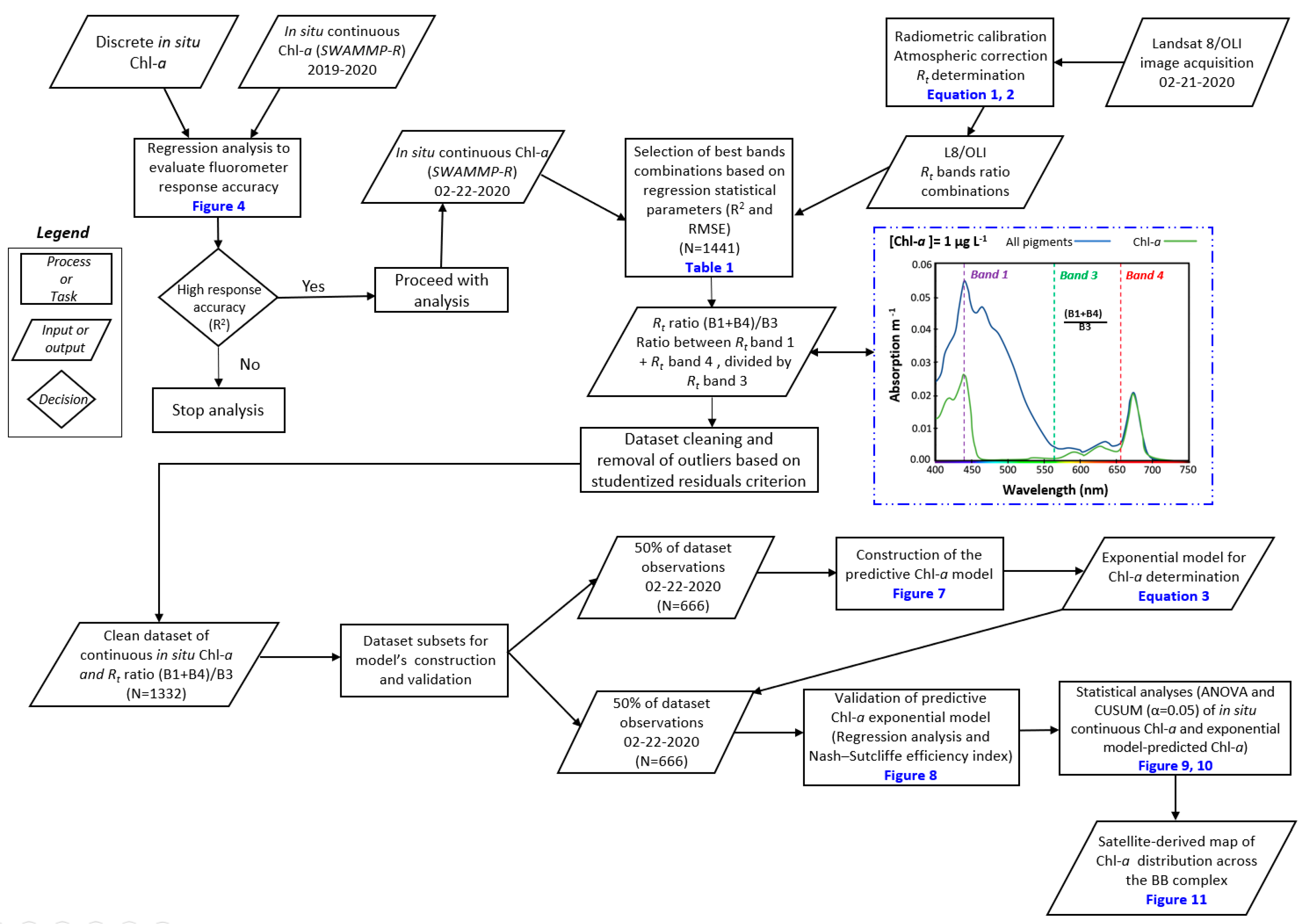
2.2.3. Satellite Imagery Acquisition and Processing

Nearly cloud-free Level-1 L8/OLI satellite imagery were downloaded from the USGS website (https://earthexplorer.usgs.gov/). L8/OLI images are geometrically corrected and are projected in the UTM (Universal Transverse Mercator) map with the WGS 84 datum. We used ENVI 5.3 (Exelis Visual Information Solutions, Boulder, CO, USA) and ArcGIS 10.5 (ESRI, Redlands, CA, USA) for image processing and to derive surface reflectance data. Image processing included a radiometric calibration to convert digital numbers (DN) from the satellite images into radiance values per pixel (units: µW/(cm² × sr × nm) and to perform the required atmospheric correction. The following formula [77] was used to convert DN to radiance values:

L_λ = M_L × Q_cal + A_L

(1)

where L_λ is the spectral radiance (W/(m² × sr × μm; top of the atmosphere radiance), M_L is the radiance multiplicative scaling factor for the selected band (RADIANCE_MULT_BAND_n from the metadata), A_L is the radiance additive scaling factor for the band (RADIANCE_ADD_BAND_n from the metadata), and Q_cal is the pixel DN value.

Atmospheric effects were removed by using the FLAASH (Fast Line-of-sight Atmospheric Analysis of Spectral Hypercubus) atmospheric correction module included in ENVI 5.3. This atmospheric correction accounts for factors that can affect the radiation detected by the satellite sensor (i.e., sky light, atmospheric sun glint, and radiance reflected by white caps; [77]) when retrieving surface reflectance (R_t) data. Previous studies have demonstrated that FLAASH is effective to determine the surface reflectance produced by water constituents [21,77,78,79]. The equation [77] to calculate surface reflectance (R_t) is:

R_t = 1 − ρe / A (L − B × (ρe/1−ρeS) − La)

(2)

where L is the spectral radiance at-sensor pixel, ρe is an average surface reflectance for the pixel and its surroundings, S is the atmospheric spherical albedo, A and B are coefficients that depend on atmospheric and geometric conditions but not on the surface, and La is the atmospheric back scattered radiance. The selected model parameters included both the atmospheric US-Standard and the maritime aerosol models to correct the L8/OLI images. Additionally, multispectral settings were readjusted for L8/OLI images, including the adjustment for open water areas based on the proximity to the water-dominated areas. The FLAASH output is the apparent reflectance data where pixel values ranging from 0 to 10,000 represent a corresponding range from 0–100% reflectance. In some cases, pixel values are outside this range as result of extremely dark/shadow areas or noise; thus, the Band Math Tool from the ENVI toolbox [80] was used to rescale the pixel’s values to a floating-point format (i.e., range 0–1).

2.2.4. Remote Sensing-based Algorithms to Estimate Chl-a Concentrations

Most of the remote sensing algorithms for Chl-a determination are based on the optical properties (i.e., sunlight absorption patterns) of algal pigment structure and quantity [21]. These empirical models were developed using regression analyses to correlate reflectance data to in situ Chl-a concentrations. Despite the simplicity of this approach, results from this statistical analysis are highly informative about water quality conditions when using Chl-a as indicator of eutrophication or levels of nutrient enrichment and potential nutrient sources. However, one of the criticisms (and limitations) is that these empirical algorithms are calibrated and validated based on a small number of in situ samples (c.a., ~20 samples) [21,81,82]. In this study, we used Level-1 Landsat 8/OLI images (path 22, rows 39 and 40) captured on 21 February 2020 and continuous in situ Chl-a fluorometry data collected approximately 20 h apart (22 February 2020; N = 1441 data observations) to increase the sample size (>1000 sampling points). Due to cloud coverage at the Barataria Bay coastal boundary, the transverse transects were not considered for the model’s calculation and validation (Figure S2). Similarly, due to geomorphological features (e.g., narrow man-made channel distribution, dredging), constructed structures (e.g., levees and gates), and hydrological variability (e.g., channel width and water depth) linked to major ecological differences (i.e., extensive floating mats of the water hyacinth (Eichhornia crassipes) and tree canopies), we excluded the Gate transect section for the model forecasting when compared to the main water bodies. Thus, for the algorithm development we used continuous in situ Chl-a data collected along salinity gradients from the most northern area of Lake Cataouatche (0.16 ± 0.01 ppt) to lower Barataria Bay (6.8 ± 5.3 ppt) (Figure S2).

L8/OLI bands were combined into different spectral bands followed by applying linear, polynomial, and exponential regression models to calculate a three bands ratio algorithm to characterize the relationship between the surface reflectance (R_t) data and the continuous in situ Chl-a (i.e., SWAMMP-R acquisition) concentrations. We used the continuous in situ Chl-a data and the best correlated R_t bands ratio combination to fit and test the model (Figure 2). After sequentially selecting the best correlated R_t bands ratio combination, the dataset was evaluated for noise and outliers due to sensor response and boat speed using studentized residuals criterion in JMP Pro 15.1.0 software [83]. This revised dataset (N = 1332) was then separated into two subsets containing half (N = 666) of the total observations for the corresponding model calibration and validation steps. To test the model predictive capabilities, we used regression analysis, analysis of variance (α = 0.05), Nash-Sutcliffe efficiency coefficient (NSE), and cumulative sum test (CUSUM). To evaluate the model predictive power, the NSE coefficient determines the residual variance compared to the observed data variance [84,85], while the CUSUM analysis helps to identify and interpret patterns in complex spatial and temporal series data [86]. Once the model validation was completed, we used the selected model equation to map Chl-a concentrations across the BB complex spatial domain (Figure 2).

3. Results

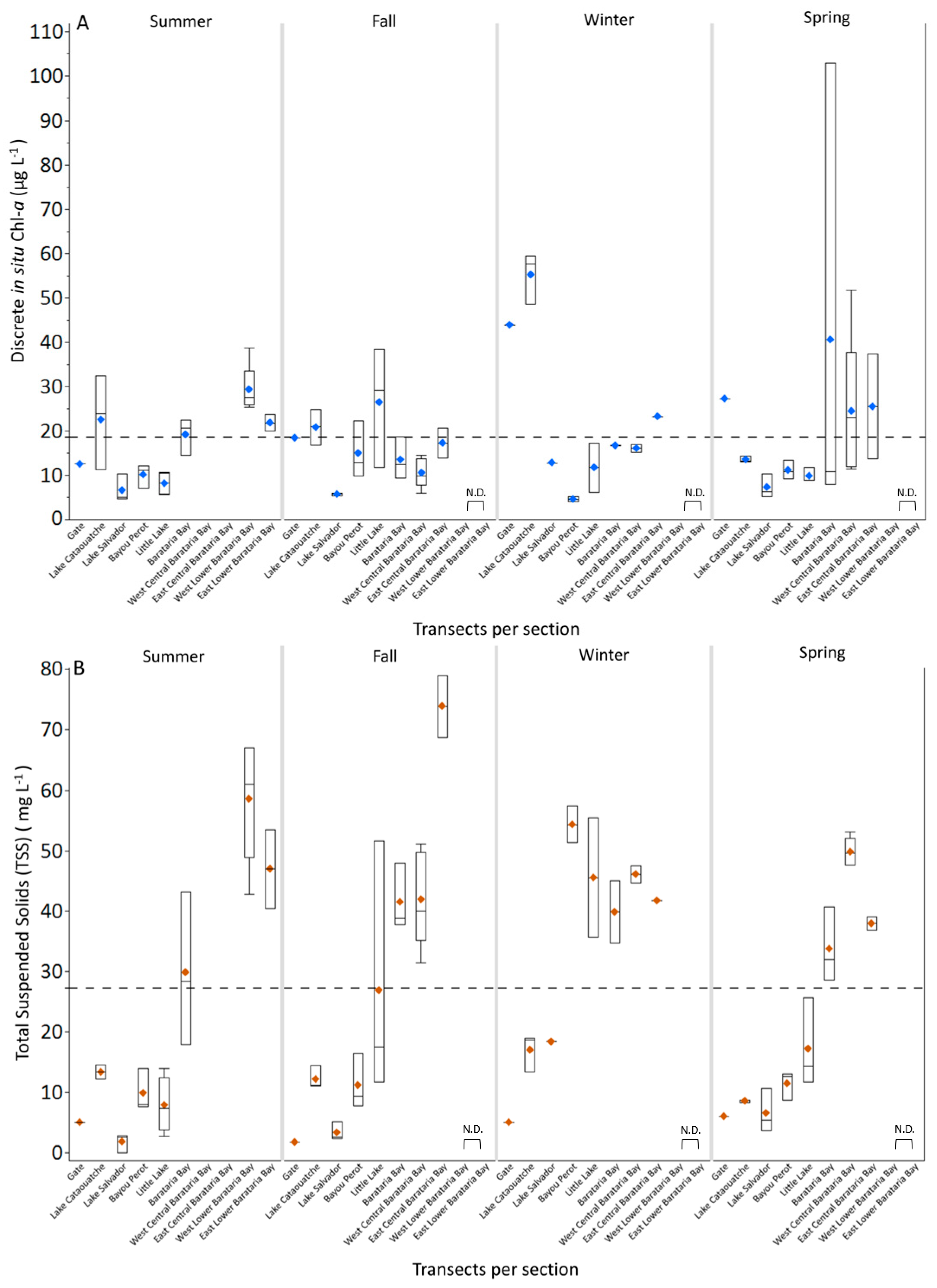
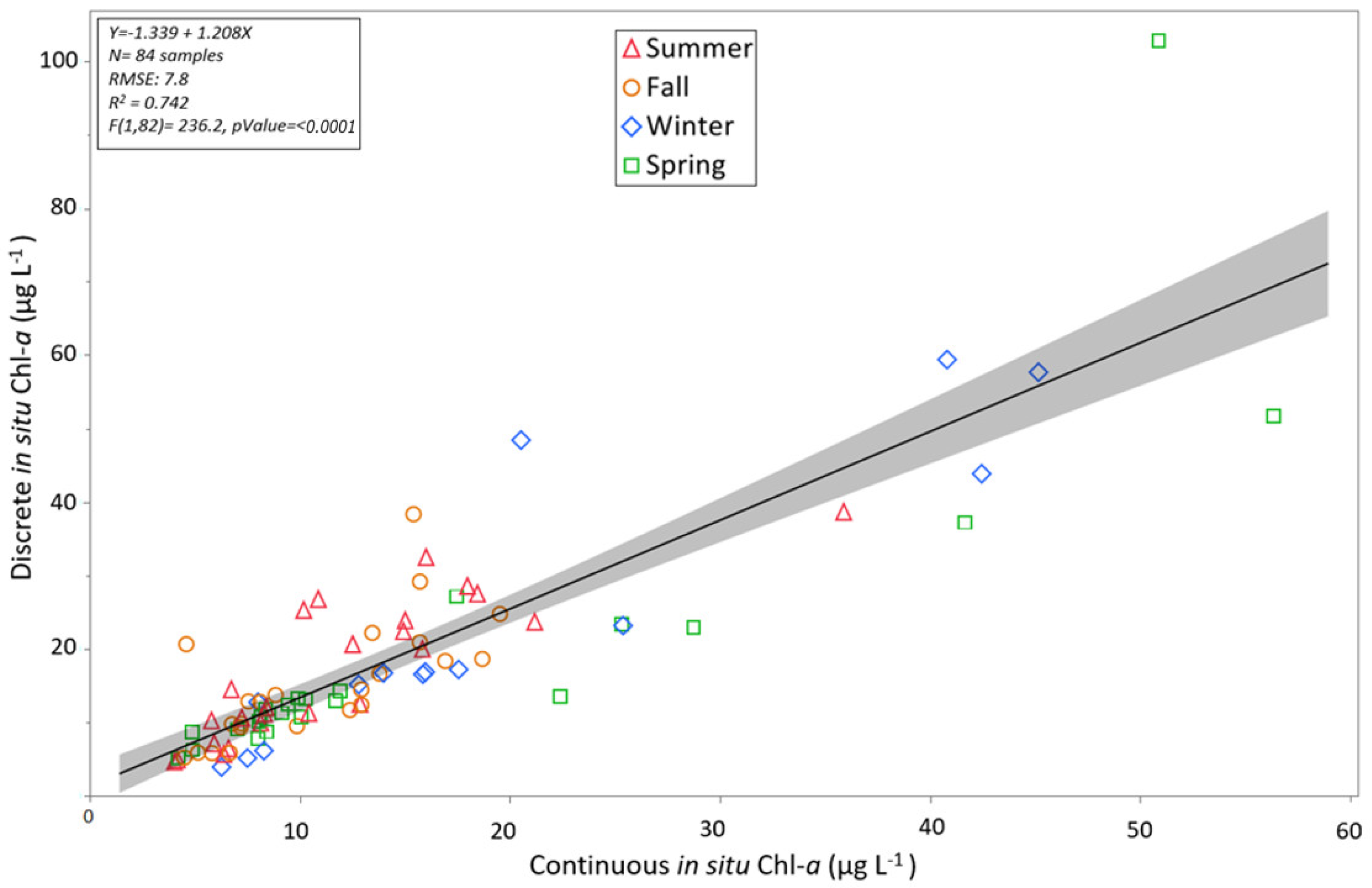
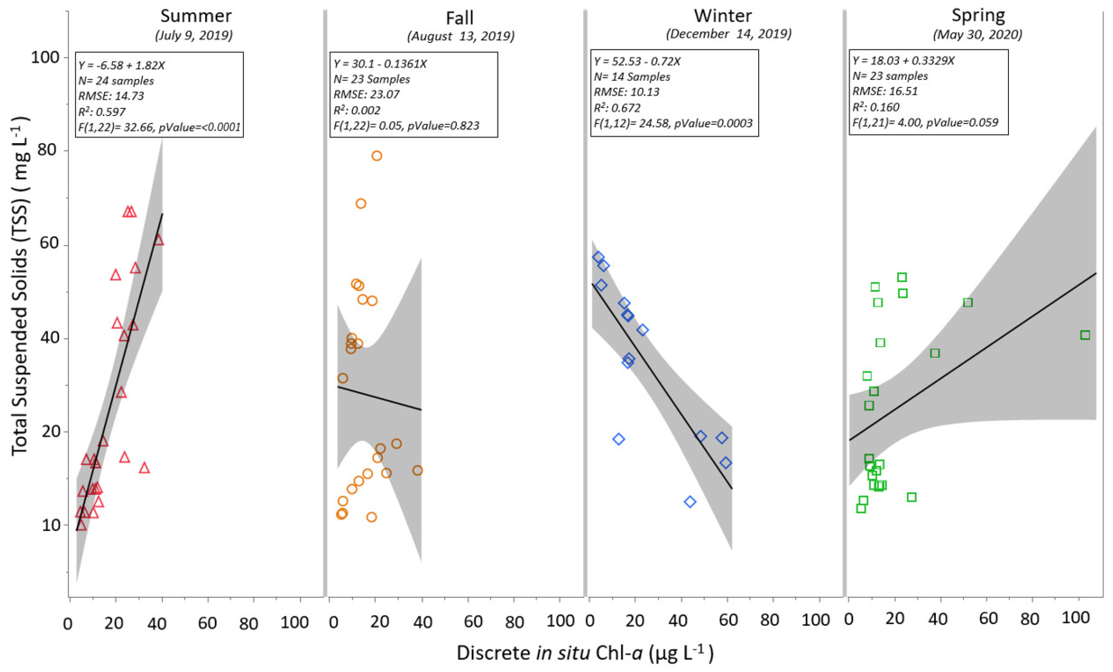
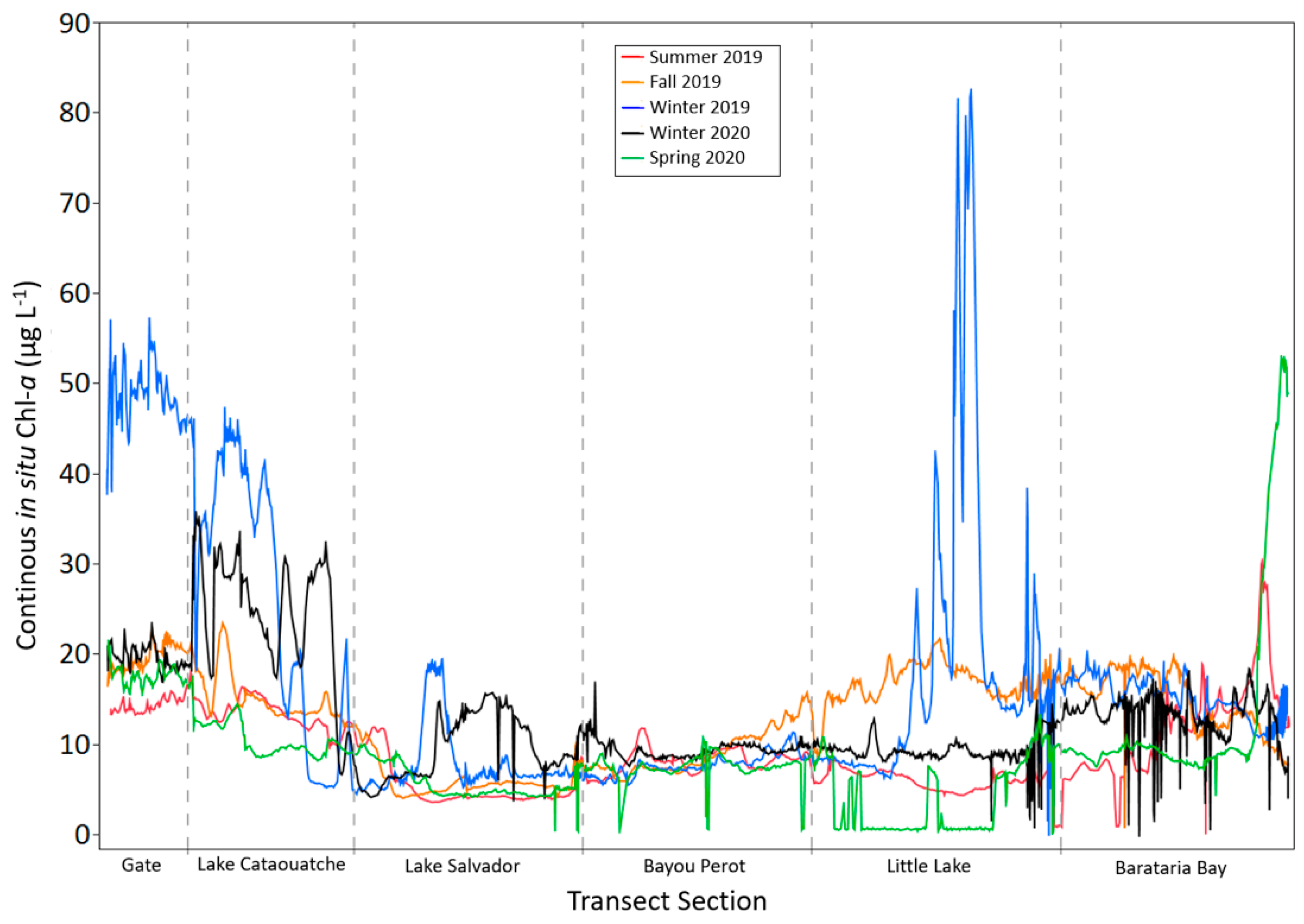
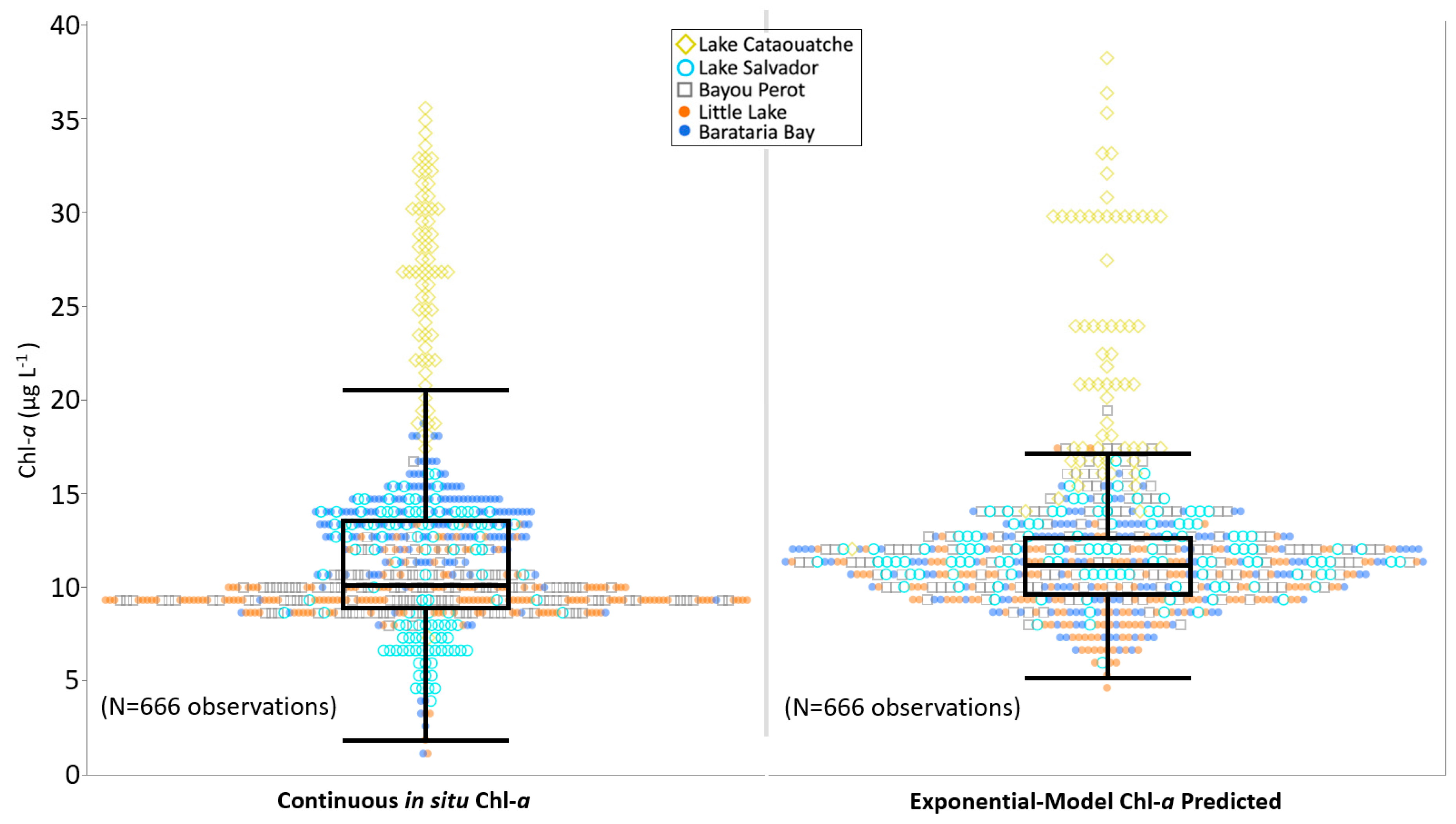
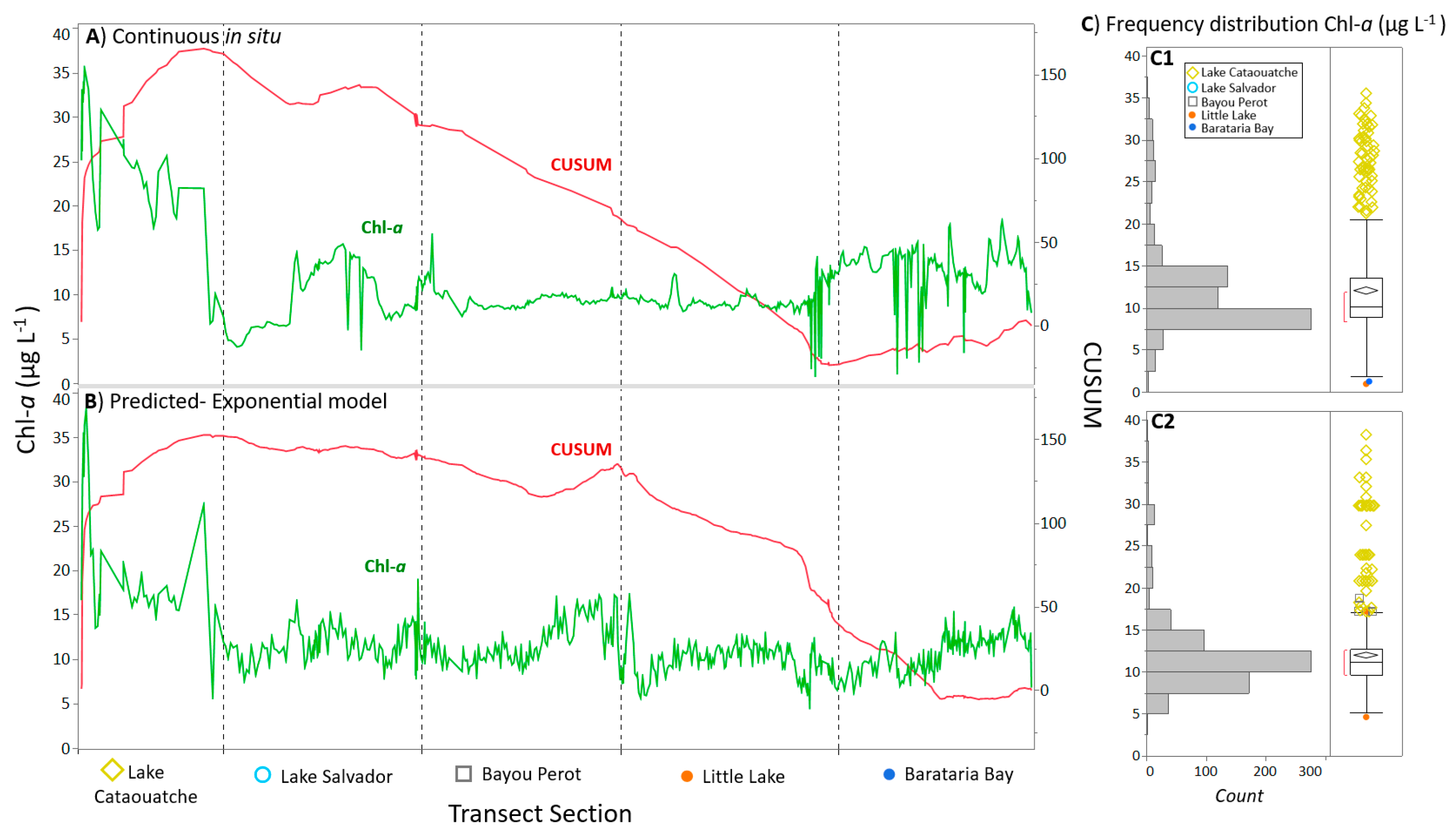
3.1. Discrete and Continuous Chl-a Data Statistical Summary

The average in situ Chl-a concentration (±SD) obtained from discrete water samples collected during the Mississippi River flood pulse (2019–2020) was 18.5 ± 15.2 SD µg L⁻¹. The lowest Chl-a value (3.97 µg L⁻¹) was measured at Bayou Perot during Winter and the highest (102.92 µg L⁻¹) along the lower Barataria Bay transect in Spring 2020 during the MR peak discharge (Figure 3A). No significant seasonal patterns were observed throughout the BB complex. However, the presence of a spatially discrete phytoplankton bloom was observed in the lower Barataria Bay during Spring 2020 near the Quatre Bayou Pass-station (Figure 3A). The average TSS concentration during the Mississippi River flood pulse (2019–2020) was 27.2 ± 20.5 SD mg L⁻¹; minimum values were observed in Lake Salvador (<1 mg L⁻¹) during summer 2019 and a maximum concentration in the east central Barataria Bay transect (79 mg L⁻¹) during fall 2019 (Figure 1 and Figure 3B).

There was a significant correlation coefficient (r = 0.86) and coefficient of determination (R² = 0.74; p < 0.0001) between the discrete in situ Chl-a values and the continuous in situ Chl-a (SWAMMP-R) values indicating that the continuous in situ Chl-a values directly measured through fluorometry techniques are robust estimations of Chl-a concentrations; thus, these values are suitable to interpolate values across the BB complex (Figure 4).

A regression analysis between TSS and Chl-a revealed seasonal patterns where Chl-a was a major constituent of particulate matter load during the summer (9 July 2019) and spring (30 May 2020) seasons (Figure 5).

During the 2019–2020 MR flood pulse the continuous in situ Chl-a data also showed consistent spatial patterns, where consistently higher Chl-a concentrations occurred at the upper basin (low salinity; 0.20 ± 0.03 SD ppt) and lower Chl-a values at the lower basin (higher salinity; 10.4 ± 5.9 SD ppt). Also, seasonal phytoplankton blooms were characterized during winter (14 December 2019) and spring (30 May 2020) when maximum continuous in situ Chl-a values were 82.4 µg L⁻¹ in Little Lake (mean: 17.8 ± 14.1 SD µg L⁻¹) and 52.8 µg L⁻¹ in Barataria Bay (mean: 14.2 ± 12.5 SD µg L⁻¹) (Figure 6).

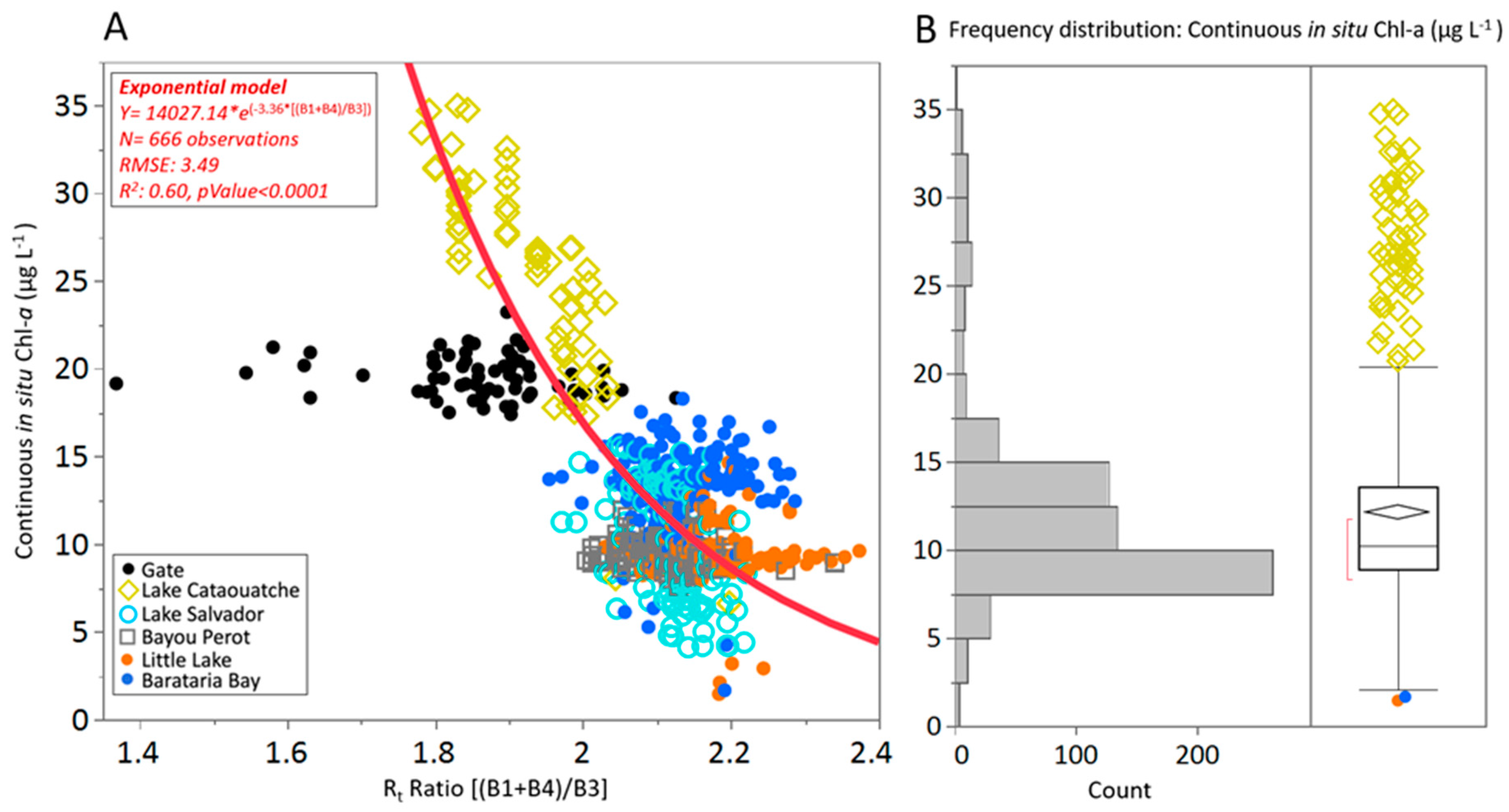
3.2. Determining the Best Band Ratio and Algorithm Development Application

Linear, polynomial, and exponential regression analyses were performed using a total of 1441 observations of continuous in situ Chl-a collected on 22 February 2020 and different ratio combinations of R_t L8/OLI bands derived from the L8/OLI satellite image acquired on 21 February 2020 (Figure 2). The best relationship between these two variables was observed using the continuous in situ Chl-a values and the ratio between the R_t bands 1, 4 and 3 (i.e., R_t Ratio (B1 + B4)/B3;

Table 1. Linear, polynomial, and exponential band regression results between continuous in situ Chl-a and L8/OLI surface reflectance data (R_t). Modeling was performed using 1441 sampling points distributed throughout the BB complex along salinity gradients collected on 22 February 2020 (see methods). R², coefficient of determination; RMSE, root mean square error. All values are significant at p < 0.0001, except when p ≤ 0.0002 (*). Bold text and numbers indicate the selected model used for spatial analysis and mapping (see Figure 8).

Bands Ratios	Average Spectrum Wavelength (nm)	Linear		Quadratic		Cubic		Quartic		Exponential
		R2	RMSE	R2	RMSE	R2	RMSE	R2	RMSE	R2	RMSE
B3/B1	560/443	0.23	5.75	0.27	5.59	0.32	5.42	0.37	5.20	0.26	5.66
B5/B2	865/480	0.17	5.99	0.19	5.91	0.21	5.84	0.23	5.75	0.19	5.93
B5/B3	865/560	0.15	6.03	0.19	5.89	0.21	5.84	0.24	5.73	0.18	5.96
B5/B4	865/655	0.12	6.17	0.17	5.99	0.19	5.92	0.20	5.86	0.14	6.09
B4/B2	655/480	0.01	6.53 *	0.01	6.53 *	0.03	6.47	0.04	6.43	0.01	6.53
B3/B2	560/480	0.05	6.39	0.09	6.25	0.09	6.25	0.11	6.21	0.06	6.37
B2/B1	480/443	0.16	6.03	0.18	5.93	0.19	5.93	0.19	5.93	0.18	5.96
B4/B1	655/443	0.02	6.48	0.04	6.43	0.05	6.41	0.08	6.30	0.03	6.47
B4/B3	655/560	0.29	5.53	0.32	5.42	0.33	5.40	0.33	5.37	0.31	5.44
B5/B1	865/443	0.12	6.17	0.16	6.02	0.19	5.92	0.19	5.92	0.13	6.11
B2/B3	480/560	0.04	6.42	0.08	6.29	0.10	6.24	0.10	6.24	0.05	6.40
B1/B2	443/480	0.14	6.08	0.17	5.97	0.19	5.92	0.19	5.93	0.17	5.99
B1/B3	443/560	0.19	5.89	0.29	5.53	0.29	5.52	0.35	5.32	0.25	5.68
(B1 + B4)/B3	(443 + 655)/560	0.39	5.12	0.50	4.66	0.50	4.63	0.54	4.47	0.46	4.80

). Band 1 is centered at 443 nm corresponding to the first Chl-a strong absorption peak; band 4 is centered at 655 nm (low point of the second Chl-a absorption peak) while band 3 is centered at 562 nm within the green range corresponding to the minimum Chl-a absorption ([87]; Figure 2). Indeed, R_t bands 1, 4 and 3 are commonly used for spectral estimates of Chl-a as these bio-physical properties strongly shape its contribution to surface reflectance [81,87].

Prior to the model calibration and validation, the full dataset (N = 1441) was evaluated for noise and outliers due to sensor response and boat speed using a studentized residuals criterion in JMP Pro 15.0.0 software (SAS Institute, Cary, NC, USA) (Figure 2). After removing outliers, the dataset (N = 1332) was divided into two subsets for model calibration (N = 666) and validation (N = 666). Overall, the proportional relationship between these two variables was best characterized using an exponential model between the continuous in situ Chl-a values and the ratio (R_t [B1 + B4]/B3), expressed as:

[Chl-a] = 14027.14 × e^{(−3.36×[(B1 + B4)/B3])}

(3)

Although more complex polynomial regression models were significant (Table 1), they were biased (data not shown) towards the lower and middle Chl-a values (~50% of the total observations; Figure 7). This bias was compounded by the spectral signature of the Gate transect data (N = 68 observations), which showed major differences in water optical properties as result of hydrology and ecological processes when compared with the rest of the water bodies in the BB complex (Figure S1). Thus, these transect values, representing ~5% of the total number of continuous in situ Chl-a values (N = 1441) collected on 22 February 2020 were excluded in the regression analysis (see Section 4).

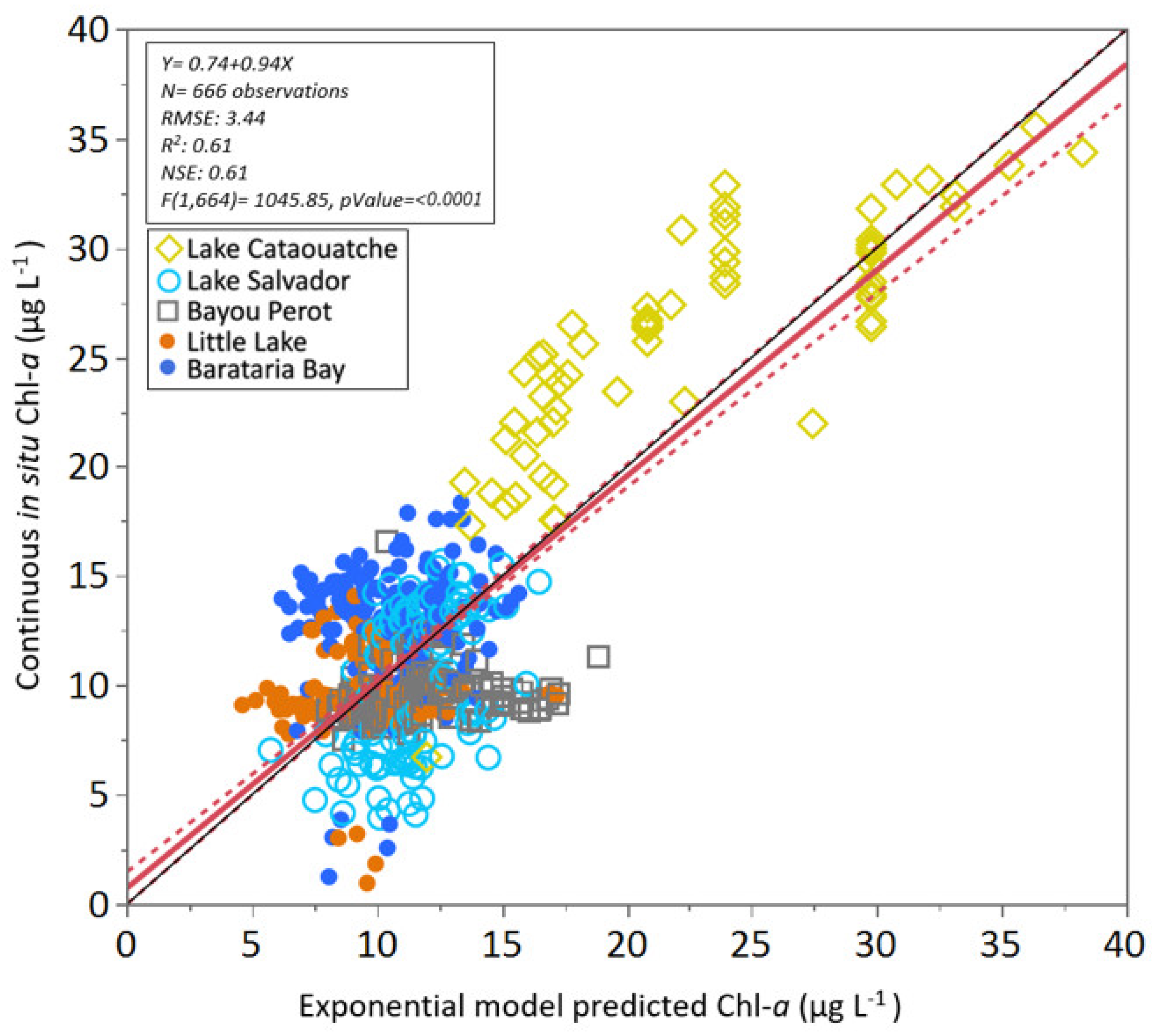
3.3. Algorithm Validation

The exponential model was statistically significant and able to predict Chl-a concentrations along the BB complex transect sections (r = 0.77). A total of 666 observations were used to validate the model predictive power (R² = 0.61; RMSE = 3.44; NSE = 0.61; p < 0.0001; Figure 8).

The Chl-a concentration was not significantly different (α = 0.05) between the continuous in situ Chl-a and the models predicted Chl-a for the entire BB complex (F(1, 1330) = 0.02, p = 0.89; Figure 9).

The selected model was able to replicate the frequency distribution of the validation dataset, where ~50% of the Chl-a observations are between 5–15 µg L⁻¹, and its predicted values were similar to the continuous in situ Chl-a values across the entire salinity gradient (Figure 10).

Chl-a concentrations were highly variable along the BB complex transects on 22nd February 2020; the highest average continuous in situ Chl-a value was recorded in Lake Cataouatche (26.60 ± 5.17 µg L⁻¹; Figure 6). Although the CUSUM test did not completely replicate the Chl-a patterns along salinity gradients, it confirmed the distinctive increase of Chl-a concentrations and presence of outliers in Lake Cataouatche (Figure 10). These spatial patterns are controlled by hydrological differences, freshwater inputs, water residence time, tidal exchange [53] among well-defined subsystems within the BB complex [52,53]. These hydrological differences control nutrient availability and transport among BB complex sub-basins, promoting high Chl-a concentrations (≥60 µg L⁻¹) in Lac des Allemands and Lake Cataouatche where the Chl-a maximum zones can be detected as plumes (Figure 11A–C).

4. Discussion

Our study demonstrated the value of using high frequency (SWAMMP-R) in situ Chl-a fluorometry-based measurements paired with Landsat 8/OLI to characterize spatially-explicit Chl-a distribution at large spatial scales throughout the BB complex. The regression model using the R_t ratio ([B1 + B4]/B3) was able to characterize Chl-a spatial patterns in water bodies with variable environmental conditions (i.e., depth, hydrology, and freshwater inputs). CUSUM analysis of continuous in situ Chl-a revealed Chl-a trends along salinity gradients with the highest average value observed in Lake Cataouatche (26.0 ± 5.3 µg L⁻¹) in the upper basin where mean salinity was 0.16 ± 0.01 ppt. The lower continuous in situ Chl-a values were registered throughout the middle basin in Little Lake (9.3 ± 1.6 µg L⁻¹; mean salinity: 0.20 ± 0.06 ppt) and the lower basin in Barataria Bay (12.8 ± 2.7 µg L⁻¹; mean salinity: 6.8 ± 5.3 ppt).

The exponential model generated Chl-a concentration patterns comparable to the continuous in situ Chl-a across the BB complex, predicting higher Chl-a concentrations in Lake Cataouatche (22.8 ± 6.6 µg L⁻¹), followed by lower values throughout the middle basin at Lake Salvador (11.6 ± 1.8 µg L⁻¹), Bayou Perot (11.8 ± 2.3 µg L⁻¹), and Little Lake (9.7 ± 1.9 µg L⁻¹) and the lower basin at Barataria Bay (10.9 ± 2.1 µg L⁻¹). The selected model also confirms that the highest Chl-a concentrations occur in the upper basin at Lac des Allemands (Figure 11B), which has been reported as a highly productive area during the last ~40 years due to major nutrient loading rates resulting from agriculture practices and urban development [29,30,47,49,88].

Due to the low correlation (R² = 0.02; p = 0.15) between TSS and Chl-a concentration (N = 84 samples), we propose that the BB complex became an optically complex system [Case 2 water; [81]] during the MR flood in 2019–2020. When this relationship was analyzed by season, we detected a positive correlation between TSS and Chl-a in spring and summer, but a negative trend in winter (Figure 5). These results suggest that Chl-a becomes the major constituent driving water color during summer and spring when nutrient concentrations, temperature and solar irradiance are high coinciding with the peak water column productivity [30,49,89,90]. Moreover, observations from both the discrete sample assays and field high-frequency fluorometry allow us to differentiate the optical properties among different water masses. We noted the most conspicuous difference in the water column along the Gate transect section, where mats of floating vegetation covered the channel surface due to the interaction of high nutrient concentrations and wind direction/velocity causing rapid plant growth and vegetation biomass accumulation. One significant difference between water masses among the Gate channel and the rest of the transects across the BB complex was the high pCO₂ concentrations in the water column (Figure S1). During the 22 February 2020 field sampling, high pCO₂ values in the Gate channel area ranged from 1459.6 to 4095.6 ppm, in contrast to the lower range (423.4–520.4) measured in the Barataria Bay transect (Figure S1). This high pCO₂ concentration reflects the high respiratory activity occurring in the narrow channel due to the decomposition of live and dead plant material (organic matter) accumulated in the channel bottom and the water column. Water oxygen concentration >3 mg L⁻¹ facilitates organic matter decomposition, releasing organic derived substances to the water column that influence the optical characteristics (i.e., surface reflectance) captured by the Landsat 8/OLI satellite in the Gate transect (Figure 7). This type of channel (i.e., narrow and running across wetland areas) is common throughout the BB complex, not only as result of natural sediment deposition patterns, but also as result of dredging for oil and gas exploration and navigation activities, particularly in the last 50 years [66].

Our analysis showed that within each season and during river flooding conditions, the average continuous in situ Chl-a concentrations are higher at the upper basin in the Gate transect (Figure 6; 26.8 ± 14.1 µg L⁻¹) and Lake Cataouatche (Figure 6; 21.8 ± 11.5 µg L⁻¹) while salinity increases in the middle of Lake Salvador (Figure 6; 7.7 ± 3.8 µg L⁻¹) and the lower Barataria Bay basins (Figure 6; 13.7 ± 6.2 µg L⁻¹). We attribute this spatial pattern to both the direct effect of the MR flood pulse, when high concentrations of inorganic nutrients enter through the DPFD into the northern region of Lake Cataouatche and the higher water residence time (>100 days; [53]) in these systems that promote high phytoplankton productivity [91]. This production pattern is similar in Lac des Allemands where the residence time is also high (50–70 days; [52,53]), and where there is also a constant input of inorganic nutrients due to runoff from surrounding sugar cane farms [49,88]. The local plume distributions of both TSS and Chl-a are clearly demarcated in both lakes as freshwater input enters in pulses, highlighting the relative importance of nutrient inputs for controlling water column primary productivity at local scales (Figure 11A–C). On the marine end-member of the salinity gradient downstream, the MR plume also enters the lower basin through tidal inlets as showed in previous studies [30,60]. This direct riverine input enters into the lower Barataria Bay during the peak of the MR discharge in combination with water currents running parallel to the adjacent continental shelf, causing an increase in Chl-a in Barataria Bay as underscored by water with high inorganic nutrient concentrations during the period from 1992 to 2016 (e.g., NO₃ + NO₂, 12.0 ± 15.2 µM) [49,92].

The interaction among the MS river discharge seasonality, differences in water residence time, and biological processes across the BB complex can influence Chl-a concentration and phytoplankton productivity. This interaction is apparent in the upper basin when nutrient loading is low during the summer [93]. Water residence time increases during the summer when the Mississippi River is at its lowest level reducing nutrient inputs into the estuary [52]. Sampling of inorganic nutrients along the transect (data not shown) indicates that water bodies in the BB complex might be nutrient limited during the summer when temperature increases, and peak phytoplankton productivity occurs. Similarly, low nitrogen concentrations have been associated with denitrification rates in benthic sediments thus promoting nitrogen limitation during the summer when denitrification rates are the highest [94,95]. Low Chl-a concentration in the upper and middle basins can also be attributed to consumption by benthic organisms where the presence of Rangia clam populations (Rangia cuneata) is extensive. Shallow water column depth and high water residence time facilitates the availability of organic matter, including phytoplankton, to benthic communities [52,96].

The observed salinity and predicted Chl-a gradients revealed well defined subsystems within the BB complex as underscored by other studies (i.e., [53]). These subsystem boundaries are supported by the high Chl-a spatial variability we documented within Lake Cataouatche when compared with Chl-a values in the middle and lower basins. Although all BB complex sections captured by our SWAMMP-R transects represent a hydrological continuum, these Chl-a patterns reveal the spatially and temporally local effects of freshwater inputs, residence time, geomorphology, and weather (i.e., precipitation, cold fronts, and major storms) as reflected by the year-round patchiness in Chl-a spatial distribution in Lake Cataouatche (Figure 6 and Figure 11B1,C1). This irregular and patchy Chl-a distribution is difficult to capture using only discrete sampling techniques along transects as shown by our results and previous studies [49,88].

The ecological responses at local/regional scales to extreme weather and climate patterns (e.g., precipitation, wind velocity and strength, tropical storms) in estuaries and lagoons along coastal Louisiana are not well understood, particularly under current climate variability. For instance, in August 2016, a stationary low pressure system caused more than 50 cm of cumulative precipitation in a three-day period affecting coastal areas in South Louisiana including record flooding levels inland [97]. This event was associated to the lowest average annual salinity recorded in 2016 during a span of 22 years (1994–2016) in the BB complex (Figure S3; [49]. Recently, the 2020 hurricane season was a record for coastal Louisiana with four major storm landfalls in one season (i.e., tropical storms and hurricanes). For example, hurricane Delta, (category-2) at the time of landfall in Creole, LA and ~335 km from the BB complex, caused a storm surge (1–1.5 m) triggering ocean water intrusion into the lower BB complex. A salinity survey using the SWAMMP-R system and performed on 18 October 2020, nine days after Delta’s landfall showed saltwater intrusion up to Lake Cataouatche where salinity increased three times the annual average when compared to measurements in previous years (Figure S4A,B); this increase in salinity underscores the regulatory pulsing control of these climate events on water quality in the BB complex.

The development of robust quantitative relationships between in situ measurements of environmental and ecological parameters and remotely sensed earth surface observations is especially useful for very dynamic ecosystems and landscapes, places characterized by high variation across broad ranges of temporal and spatial scales. Our exponential model (Equation (3)) reflects this complex environmental signature across the distinctive water bodies that form part of the BB complex. This strategy for the developing of empirical models has been widely used for specific conditions, regions and even for large scale ocean color descriptions including hypertrophic water systems (West Lake-Vietnam; [21]), highly turbid lakes and coastal waters (Dnieper river, Changjiang estuary; [98,99]), freshwater lakes (Great Lakes; [100]), coastal water areas (Florida shelf; [101]), and open ocean waters [102,103].

In open ocean waters, satellite images have been used to retrieve water quality data since the late 1970′s when the Coastal Zone Color Scanner satellite (CZCS) was launched in 1978 [81]. The main limitation for the development of robust algorithms, particularly for coastal areas (e.g., [92]), is the lack or reduced number of in situ observations to train and validate these quantitative models. While previous studies have demonstrated the potential use of Landsat 8/OLI hyperspectral data to determine Chl-a, few direct field measurements (N < 25) are available to validate satellite algorithms in large study areas (e.g., 97 km²) [104]. We addressed this limitation by increasing the number of in situ Chl-a values (N = 1332) used in model calibration and validation by acquiring continuous in situ Chl-a field fluorometry measurements across the BB complex (open water area ~1903 km²; [52]).

The development of new technologies and improvement of existing instrumentation open wide possibilities for monitoring water quality at large spatial and temporal scales, while also allowing the characterization of hydrological and biochemical processes at local scales. We anticipate enhanced understanding of critical ecosystem processes like primary productivity and biomass (i.e., Chl-a), that are driven by pulsing events such as cold fronts, river discharge, and storm surges after hurricane passage on primary productivity and biomass (i.e., Chl-a). In this study we showed that linking Landsat 8/OLI sensor observations, with a high frequency environmental sampling approach is a powerful strategy to develop effective and robust algorithms for the assessment of both water quality and optical properties. This is especially useful in spatially large-scale and highly dynamic estuarine systems (i.e., “Case 2” waters; [22,23,92]) like those found in the Mississippi River delta plain, where intricate physical and ecological dynamics cannot be captured by discrete sampling alone.

5. Conclusions

Our results demonstrated that the use of Landsat 8/OLI images provided reliable results to characterize the spatiotemporal Chl-a patterns in the Barataria Bay complex, a hydrologically delta-dominated coastal ecosystem. An exponential model was validated to evaluate Chl-a seasonal and spatial distribution using an intense acquisition of fluorometry measurements and a reflectance R_t ratio ([B1 + B4]/B3) from Landsat 8/OLI imagery/data. These results are supported by contemporary and historical data, especially the effects of local environmental variables controlling Chl-a spatial distribution and magnitude. Model interpolation and predictions showed that higher phytoplankton concentrations (i.e., Chl-a) are extensive and persistent in the upper basin, partially due to significant nutrient loadings from extensive agricultural lands and from the MR discharge through the seasonal and pulsing DPFD delivery. Our findings complement previous studies in which salinity is used as a proxy to characterize well-defined subsystems within the BB complex, and where despite the hydrological connectivity, distinctive biochemical processes, and productivity patterns define each subsystem. To further expand the validation of Chl-a spatiotemporal patterns using our proposed algorithm, we recommend the analysis of historical and new Landsat 8/OLI data to assess past, current, and future ecological and hydrodynamic changes. This is particularly pressing from a management perspective, since this deltaic estuarine system is undergoing large-scale hydrological restoration as it experiences increasing rates of relative sea level rise and wetland loss as a result of human disturbances, hurricane impacts, and climate change [105,106].

References

1. Bianchi, T.S. Biogeochemistry of Estuaries; Oxford University Press on Demand: Oxford, UK, 2007. [Google Scholar]
2. Teichert, N.; Borja, A.; Chust, G.; Uriarte, A.; Lepage, M. Restoring fish ecological quality in estuaries: Implication of interactive and cumulative effects among anthropogenic stressors. Sci. Total Environ. 2016, 542, 383–393. [Google Scholar] [CrossRef]
3. Vasconcelos, R.P.; Reis-Santos, P.; Fonseca, V.; Maia, A.; Ruano, M.; França, S.; Vinagre, C.; Costa, M.J.; Cabral, H. Assessing anthropogenic pressures on estuarine fish nurseries along the Portuguese coast: A multi-metric index and conceptual approach. Sci. Total Environ. 2007, 374, 199–215. [Google Scholar] [CrossRef] [PubMed]
4. Arend, K.K.; Beletsky, D.; DePinto, J.V.; Ludsin, S.A.; Roberts, J.J.; Rucinski, D.K.; Scavia, D.; Schwab, D.J.; Höök, T.O. Seasonal and interannual effects of hypoxia on fish habitat quality in central Lake Erie. Freshw. Biol. 2011, 56, 366–383. [Google Scholar] [CrossRef] [Green Version]
5. O’Hare, M.T.; Baattrup-Pedersen, A.; Baumgarte, I.; Freeman, A.; Gunn, I.D.; Lázár, A.N.; Sinclair, R.; Wade, A.J.; Bowes, M.J. Responses of aquatic plants to eutrophication in rivers: A revised conceptual model. Front. Plant Sci. 2018, 9, 451. [Google Scholar] [CrossRef]
6. Smith, V.H. Eutrophication of freshwater and coastal marine ecosystems a global problem. Environ. Sci. Pollut. Res. 2003, 10, 126–139. [Google Scholar] [CrossRef] [PubMed]
7. Turner, R.E.; Rabalais, N.N. Coastal eutrophication near the Mississippi river delta. Nature 1994, 368, 619–621. [Google Scholar] [CrossRef]
8. Walker, N.D.; Rabalais, N.N. Relationships among satellite chlorophylla, river inputs, and hypoxia on the Louisiana Continental shelf, Gulf of Mexico. Estuaries Coasts 2006, 29, 1081–1093. [Google Scholar] [CrossRef]
9. Bricker, S.; Longstaff, B.; Dennison, W.; Jones, A.; Boicourt, K.; Wicks, C.; Woerner, J. Effects of nutrient enrichment in the nation’s estuaries: A decade of change. In NOAA Coastal Ocean Program Decision Analysis Series No. 26; National Ocean Service: Silver Spring, MD, USA, 2007; p. 328. [Google Scholar]
10. Bricker, S.; Clement, C.; Pirhalla, D.; Orlando, S.; Farrow, D. National estuarine eutrophication assessment. In Effects of Nutrient Enrichment in the Nation’s Estuaries; NOAA, National Ocean Service: Silver Spring, MD, USA, 1999; p. 71. [Google Scholar]
11. Howarth, R.W.; Swaney, D.P.; Butler, T.J.; Marino, R. Rapid communication: Climatic control on eutrophication of the Hudson River Estuary. Ecosystems 2000, 3, 210–215. [Google Scholar] [CrossRef]
12. James, N.C.; van Niekerk, L.; Whitfield, A.K.; Potts, W.M.; Götz, A.; Paterson, A.W. Effects of climate change on South African estuaries and associated fish species. Clim. Res. 2013, 57, 233–248. [Google Scholar] [CrossRef] [Green Version]
13. Statham, P.J. Nutrients in estuaries—an overview and the potential impacts of climate change. Sci. Total Environ. 2012, 434, 213–227. [Google Scholar] [CrossRef]
14. Bricker, S.B.; Longstaff, B.; Dennison, W.; Jones, A.; Boicourt, K.; Wicks, C.; Woerner, J. Effects of nutrient enrichment in the nation’s estuaries: A decade of change. Harmful Algae 2008, 8, 21–32. [Google Scholar] [CrossRef]
15. Painting, S.J.; Devlin, M.J.; Malcolm, S.J.; Parker, E.R.; Mills, D.K.; Mills, C.; Tett, P.; Wither, A.; Burt, J.; Jones, R.; et al. Assessing the impact of nutrient enrichment in estuaries: Susceptibility to eutrophication. Mar. Pollut. Bull. 2007, 55, 74–90. [Google Scholar] [CrossRef]
16. Carpenter, S.R. Phosphorus control is critical to mitigating eutrophication. Proc. Natl. Acad. Sci. USA 2008, 105, 11039–11040. [Google Scholar] [CrossRef] [Green Version]
17. Conley, D.J.; Paerl, H.W.; Howarth, R.W.; Boesch, D.F.; Seitzinger, S.P.; Havens, K.E.; Lancelot, C.; Likens, G.E. Controlling eutrophication: Nitrogen and phosphorus. Science 2009, 323, 1014–1015. [Google Scholar] [CrossRef]
18. Huot, Y.; Babin, M. Overview of fluorescence protocols: Theory, basic concepts, and practice. In Chlorophyll a Fluorescence in Aquatic Sciences: Methods and Applications; Springer: Berlin/Heidelberg, Germany, 2010; pp. 31–74. [Google Scholar]
19. Laney, S.R. In situ measurement of variable fluorescence transients. In Chlorophyll a Fluorescence in Aquatic Sciences: Methods and Applications; Springer: Berlin/Heidelberg, Germany, 2010; pp. 19–30. [Google Scholar]
20. Pan, Y.; Qiu, L. A Submersible in-Situ Highly Sensitive Chlorophyll Fluorescence Detection System. In IOP Conference Series: Materials Science and Engineering; IOP Publishing: Bristol, UK, 2019; p. 022065. [Google Scholar]
21. Ha, N.T.T.; Koike, K.; Nhuan, M.T.; Canh, B.D.; Thao, N.T.P.; Parsons, M. Landsat 8/OLI two bands ratio algorithm for chlorophyll-a concentration mapping in hypertrophic waters: An application to West Lake in Hanoi (Vietnam). IEEE J. Sel. Top. Appl. Earth Obs. Remote Sens. 2017, 10, 4919–4929. [Google Scholar] [CrossRef]
22. Darecki, M.; Weeks, A.; Sagan, S.; Kowalczuk, P.; Kaczmarek, S. Optical characteristics of two contrasting Case 2 waters and their influence on remote sensing algorithms. Cont. Shelf Res. 2003, 23, 237–250. [Google Scholar] [CrossRef]
23. Moses, W.J.; Gitelson, A.A.; Berdnikov, S.; Povazhnyy, V. Estimation of chlorophyll-a concentration in case II waters using MODIS and MERIS data—successes and challenges. Environ. Res. Lett. 2009, 4, 045005. [Google Scholar] [CrossRef] [Green Version]
24. Babin, M.; Morel, A.; Gentili, B. Remote sensing of sea surface sun-induced chlorophyll fluorescence: Consequences of natural variations in the optical characteristics of phytoplankton and the quantum yield of chlorophyll a fluorescence. Int. J. Remote Sens. 1996, 17, 2417–2448. [Google Scholar] [CrossRef]
25. Schallenberg, C.; Lewis, M.R.; Kelley, D.E.; Cullen, J.J. Inferred influence of nutrient availability on the relationship between Sun-induced chlorophyll fluorescence and incident irradiance in the Bering Sea. J. Geophys. Res. Ocean. 2008, 113. [Google Scholar] [CrossRef] [Green Version]
26. Xing, X.; Claustre, H.; Blain, S.; d’Ortenzio, F.; Antoine, D.; Ras, J.; Guinet, C. Quenching correction for in vivo chlorophyll fluorescence acquired by autonomous platforms: A case study with instrumented elephant seals in the Kerguelen region (Southern Ocean). Limnol. Oceanogr. Methods 2012, 10, 483–495. [Google Scholar] [CrossRef] [Green Version]
27. Cui, T.; Zhang, J.; Wang, K.; Wei, J.; Mu, B.; Ma, Y.; Zhu, J.; Liu, R.; Chen, X. Remote sensing of chlorophyll a concentration in turbid coastal waters based on a global optical water classification system. ISPRS J. Photogramm. Remote Sens. 2020, 163, 187–201. [Google Scholar] [CrossRef]
28. Schaeffer, B.A.; Hagy, J.D.; Conmy, R.N.; Lehrter, J.C.; Stumpf, R.P. An Approach to Developing Numeric Water Quality Criteria for Coastal Waters Using the SeaWiFS Satellite Data Record. Environ. Sci. Technol. 2012, 46, 916–922. [Google Scholar] [CrossRef]
29. Hopkinson, C.S.; Day, J.W. Aquatic productivity and water quality at the upland-estuary interface in Barataria Basin, Louisiana. In Ecological Processes in Coastal and Marine Systems; Springer: Berlin/Heidelberg, Germany, 1979; pp. 291–314. [Google Scholar]
30. Ren, L.; Rabalais, N.N.; Turner, R.E.; Morrison, W.; Mendenhall, W. Nutrient limitation on phytoplankton growth in the upper Barataria Basin, Louisiana: Microcosm bioassays. Estuaries Coasts 2009, 32, 958–974. [Google Scholar] [CrossRef]
31. Bargu, S.; Justic, D.; White, J.R.; Lane, R.; Day, J.; Paerl, H.; Raynie, R. Mississippi River diversions and phytoplankton dynamics in deltaic Gulf of Mexico estuaries: A review. Estuar. Coast. Shelf Sci. 2019, 221, 39–52. [Google Scholar] [CrossRef]
32. Elsey-Quirk, T.; Graham, S.A.; Mendelssohn, I.A.; Snedden, G.; Day, J.W.; Twilley, R.; Shaffer, G.; Sharp, L.; Pahl, J.; Lane, R. Mississippi river sediment diversions and coastal wetland sustainability: Synthesis of responses to freshwater, sediment, and nutrient inputs. Estuar. Coast. Shelf Sci. 2019, 221, 170–183. [Google Scholar] [CrossRef]
33. Wang, H.; Steyer, G.D.; Couvillion, B.R.; Rybczyk, J.M.; Beck, H.J.; Sleavin, W.J.; Meselhe, E.A.; Allison, M.A.; Boustany, R.G.; Fischenich, C.J. Forecasting landscape effects of Mississippi River diversions on elevation and accretion in Louisiana deltaic wetlands under future environmental uncertainty scenarios. Estuar. Coast. Shelf Sci. 2014, 138, 57–68. [Google Scholar] [CrossRef]
34. White, J.R.; Delaune, R.D.; Justic, D.; Day, J.W.; Pahl, J.; Lane, R.R.; Boynton, W.R.; Twilley, R.R. Consequences of Mississippi River diversions on nutrient dynamics of coastal wetland soils and estuarine sediments: A review. Estuar. Coast. Shelf Sci. 2019, 224, 209–216. [Google Scholar] [CrossRef]
35. Das, A.; Justic, D.; Inoue, M.; Hoda, A.; Huang, H.; Park, D. Impacts of Mississippi River diversions on salinity gradients in a deltaic Louisiana estuary: Ecological and management implications. Estuar. Coast. Shelf Sci. 2012, 111, 17–26. [Google Scholar] [CrossRef]
36. Spera, A.C.; White, J.R.; Corstanje, R. Spatial and temporal changes to a hydrologically-reconnected coastal wetland: Implications for restoration. Estuar. Coast. Shelf Sci. 2020, 238, 106728. [Google Scholar] [CrossRef]
37. CPRA. Louisiana’s Comprehensive Master Plan for a Sustainable Coast; CPRA, Ed.; CPRA: Baton Rouge, LA, USA, 2017; p. 184. [Google Scholar]
38. Hiatt, M.; Snedden, G.; Day, J.W.; Rohli, R.V.; Nyman, J.A.; Lane, R.; Sharp, L.A. Drivers and impacts of water level fluctuations in the Mississippi River delta: Implications for delta restoration. Estuar. Coast. Shelf Sci. 2019, 224, 117–137. [Google Scholar] [CrossRef]
39. Green, M. Coastal Restoration Annual Project Reviews: December 2006. Natural Resources Department: Baton Rouge, LA, USA, 2006. [Google Scholar]
40. Lohrenz, S.E.; Dagg, M.J.; Whitledge, T.E. Enhanced primary production at the plume/oceanic interface of the Mississippi River. Cont. Shelf Res. 1990, 10, 639–664. [Google Scholar] [CrossRef]
41. Prasad, K.S.; Lohrenz, S.E.; Redalje, D.G.; Fahnenstiel, G.L. Primary production in the Gulf of Mexico coastal waters using “remotely-sensed” trophic category approach. Cont. Shelf Res. 1995, 15, 1355–1368. [Google Scholar] [CrossRef]
42. Tunnell, J., Jr.; Felder, D.; Earle, S. The Gulf of Mexico past, present, and future: A United States, Mexico, and Cuba Collaboration. In Environmental Analysis of the Gulf of Mexico; Caso, M., Pisanty, L., Ezcurra, E., Eds.; Special Publication Series; Diagnóstico Ambiental del Golfo de México; Instituto Nacional de Ecología (INE-SEMARNAT): México, Mexico, 2004; pp. 222–229. [Google Scholar]
43. Cai, W.-J.; Guo, X.; Chen, C.-T.A.; Dai, M.; Zhang, L.; Zhai, W.; Lohrenz, S.E.; Yin, K.; Harrison, P.J.; Wang, Y. A comparative overview of weathering intensity and HCO3− flux in the world’s major rivers with emphasis on the Changjiang, Huanghe, Zhujiang (Pearl) and Mississippi Rivers. Cont. Shelf Res. 2008, 28, 1538–1549. [Google Scholar] [CrossRef]
44. Kammerer, J.C. Largest rivers in the United States. In Water Resources Investigations Open File Report 87-242; U.S. Geological Survey: Reston, VA, USA, 1987; p. 2. [Google Scholar]
45. Milliman, J.D.; Meade, R.H. World-wide delivery of river sediment to the oceans. J. Geol. 1983, 91, 1–21. [Google Scholar] [CrossRef]
46. Byrnes, M.R.; Britsch, L.D.; Berlinghoff, J.L.; Johnson, R.; Khalil, S. Recent subsidence rates for Barataria Basin, Louisiana. Geo-Mar. Lett. 2019, 39, 265–278. [Google Scholar] [CrossRef]
47. Conner, W.H.; Day, J.W. The ecology of Barataria Basin, Louisiana: An Estuarine Profile; National Wetlands Research Center, US Fish and Wildlife Service, US: Washington, DC, USA, 1987; Volume 85. [Google Scholar]
48. Feijtel, T.; DeLaune, R.; Patrick, W., Jr. Carbon flow in coastal Louisiana. Mar. Ecol. Prog. Ser. 1985, 24, 255–260. [Google Scholar] [CrossRef]
49. Turner, R.E.; Swenson, E.M.; Milan, C.S.; Lee, J.M. Spatial variations in Chlorophyll a, C, N, and P in a Louisiana estuary from 1994 to 2016. Hydrobiologia 2019, 834, 131–144. [Google Scholar] [CrossRef] [Green Version]
50. Liu, B.; D’Sa, E.J.; Joshi, I. Multi-decadal trends and influences on dissolved organic carbon distribution in the Barataria Basin, Louisiana from in-situ and Landsat/MODIS observations. Remote Sens. Environ. 2019, 228, 183–202. [Google Scholar] [CrossRef]
51. Wissel, B.; Gaçe, A.; Fry, B. Tracing river influences on phytoplankton dynamics in two Louisiana estuaries. Ecology 2005, 86, 2751–2762. [Google Scholar] [CrossRef]
52. Das, A. Modeling the Impacts of Pulsed Riverine Inflows on Hydrodynamics and Water Quality in the Barataria Bay Estuary. Ph.D. Thesis, Louisiana State University, Baton Rouge, LA, USA, 2010. [Google Scholar]
53. Habib, E.; Nuttle, W.K.; Rivera-Monroy, V.H.; Gautam, S.; Wang, J.; Meselhe, E.; Twilley, R.R. Assessing effects of data limitations on salinity forecasting in Barataria basin, Louisiana, with a Bayesian analysis. J. Coast. Res. 2007, 2007, 749–763. [Google Scholar] [CrossRef]
54. Li, C.; White, J.R.; Chen, C.; Lin, H.; Weeks, E.; Galvan, K.; Bargu, S. Summertime tidal flushing of Barataria Bay: Transports of water and suspended sediments. J. Geophys. Res. Ocean. 2011, 116, 1–15. [Google Scholar] [CrossRef]
55. Walker, N.D.; Hammack, A.B. Impacts of winter storms on circulation and sediment transport: Atchafalaya-Vermilion Bay region, Louisiana, USA. J. Coast. Res. 2000, 16, 996–1010. [Google Scholar]
56. Cao, Y.; Li, C.; Dong, C. Atmospheric Cold Front-Generated Waves in the Coastal Louisiana. J. Mar. Sci. Eng. 2020, 8, 900. [Google Scholar] [CrossRef]
57. Mortimer, E.B.; Johnson, G.A.; Lau, H.W. Major Arctic outbreaks affecting Louisiana. Natl. Weather Dig. 1988, 13, 5–14. [Google Scholar]
58. Swenson, E.; Swarzenski, C. Water levels and salinity in the Barataria-Terrebonne estuarine system. In Status and Historical Trends of Hydrologic Modification, Reduction in Sediment Availability, and Habitat Loss/Modification in the Barataria and Terrebonne Estuarine Systems; BTNEP: Thibodaux, LA, USA, 1995; Volume 20, pp. 129–201. [Google Scholar]
59. Snedden, G. River, Tidal and Wind Interactions in a Deltaic Estuarine System. Ph.D. Thesis, Louisiana State University, Baton Rouge, LA, USA, 2006. [Google Scholar]
60. Sorourian, S.; Huang, H.; Li, C.; Justic, D.; Payandeh, A.R. Wave dynamics near Barataria Bay tidal inlets during spring–summer time. Ocean Model. 2020, 147, 101553. [Google Scholar] [CrossRef]
61. Wiseman, W.; Swenson, E.M.; Power, J. Salinity trends in Louisiana estuaries. Estuaries 1990, 13, 265–271. [Google Scholar] [CrossRef]
62. Marmer, H.A. The Currents in Barataria Bay; Texas A&M Research Foundation: College Station, TX, USA, 1948. [Google Scholar]
63. Bianchi, T.S.; Cook, R.L.; Perdue, E.M.; Kolic, P.E.; Green, N.; Zhang, Y.; Smith, R.W.; Kolker, A.S.; Ameen, A.; King, G. Impacts of diverted freshwater on dissolved organic matter and microbial communities in Barataria Bay, Louisiana, USA. Mar. Environ. Res. 2011, 72, 248–257. [Google Scholar] [CrossRef]
64. Kesel, R. Human modifications to the sediment regime of the Lower Mississippi River flood plain. Geomorphology 2003, 56, 325–334. [Google Scholar] [CrossRef]
65. Couvillion, B.R.; Beck, H.; Schoolmaster, D.; Fischer, M. Land Area Change in Coastal Louisiana (1932 to 2016); 2329-132X; US Geological Survey: Reston, VA, USA, 2017.
66. Day, J.; Clark, H.; Chang, C.; Hunter, R.; Norman, C. Life cycle of oil and gas fields in the Mississippi River Delta: A review. Water 2020, 12, 1492. [Google Scholar] [CrossRef]
67. Jenkins, J.A.; Olivier, H.M.; Draugelis-Dale, R.O.; Kaller, M.D. Davis Pond Freshwater Diversion Biomonitoring: Prediversion and Postdiversion Freshwater Fish Data; 2327-638X; US Geological Survey: Reston, VA, USA, 2012.
68. Penland, S.; Beall, A.D.; Britsch III, L.D. Geologic classification of coastal land loss between 1932 and 1990 in the Mississippi River Delta Plain, southeastern Louisiana. Trans. Gulf Coast Assoc. Geol. Soc. 2002, 52, 799–807. [Google Scholar]
69. Turner, R.E. Wetland loss in the northern Gulf of Mexico: Multiple working hypotheses. Estuaries 1997, 20, 1–13. [Google Scholar] [CrossRef]
70. Zhang, W.; White, J.; DeLaune, R. Diverted Mississippi River sediment as a potential phosphorus source affecting coastal Louisiana water quality. J. Freshw. Ecol. 2012, 27, 575–586. [Google Scholar] [CrossRef]
71. Lane, R.R.; Day Jr, J.W.; Marx, B.D.; Reyes, E.; Hyfield, E.; Day, J.N. The effects of riverine discharge on temperature, salinity, suspended sediment and chlorophyll a in a Mississippi delta estuary measured using a flow-through system. Estuar. Coast. Shelf Sci. 2007, 74, 145–154. [Google Scholar] [CrossRef]
72. Madden, C.J.; Day, J.W. An instrument system for high-speed mapping of chlorophyll a and physico-chemical variables in surface waters. Estuaries 1992, 15, 421–427. [Google Scholar] [CrossRef]
73. Rivera-Monroy, V.H.; Twilley, R.R.; Mancera-Pineda, J.E.; Madden, C.J.; Alcantara-Eguren, A.; Moser, E.B.; Jonsson, B.F.; Castañeda-Moya, E.; Casas-Monroy, O.; Reyes-Forero, P. Salinity and chlorophyll a as performance measures to rehabilitate a mangrove-dominated deltaic coastal region: The Ciénaga Grande de Santa Marta–Pajarales Lagoon Complex, Colombia. Estuaries Coasts 2011, 34, 1–19. [Google Scholar] [CrossRef]
74. Stachelek, J.; Madden, C.J. Application of inverse path distance weighting for high-density spatial mapping of coastal water quality patterns. Int. J. Geogr. Inf. Sci. 2015, 29, 1240–1250. [Google Scholar] [CrossRef] [Green Version]
75. Carroll, M.; Chigounis, D.; Gilbert, S.; Gundersen, K.; Hayashi, K.; Janzen, C.; Johengen, T.; Koles, T.; Laurier, F.; McKissack, T.; et al. Performance Verification Statement for the TURNER Designs CYCLOPS-7 fluorometer. Solomonsmdalliance Coast. Technol. 2005, 37. [Google Scholar] [CrossRef]
76. Arar, E.J.; Collins, G.B. Method 445.0: In Vitro Determination of Chlorophyll a and Pheophytin a in Marine and Freshwater Algae by Fluorescence; United States Environmental Protection Agency, Office of Research and Development: Cincinnati, OH, USA, 1997.
77. Chen, J.; Zhu, W.-N.; Tian, Y.Q.; Yu, Q. Estimation of colored dissolved organic matter from Landsat-8 imagery for complex inland water: Case study of Lake Huron. IEEE Trans. Geosci. Remote Sens. 2017, 55, 2201–2212. [Google Scholar] [CrossRef]
78. Joshi, I.; D’Sa, E.J. Seasonal variation of colored dissolved organic matter in Barataria Bay, Louisiana, using combined Landsat and field data. Remote Sens. 2015, 7, 12478–12502. [Google Scholar] [CrossRef] [Green Version]
79. Kutser, T.; Pierson, D.C.; Kallio, K.Y.; Reinart, A.; Sobek, S. Mapping lake CDOM by satellite remote sensing. Remote Sens. Environ. 2005, 94, 535–540. [Google Scholar] [CrossRef]
80. Nezhad, M.M.; Groppi, D.; Marzialetti, P.; Laneve, G. A sediment detection analysis with multi sensor satellites: Caspian Sea and Persian Gulf case studies. In Proceedings of the 4th World Congress on Civil, Structural, and Environmental Engineering, CSEE, Rome, Italy, 7–9 April 2019. [Google Scholar]
81. Flores-Anderson, A.I.; Griffin, R.; Dix, M.; Romero-Oliva, C.S.; Ochaeta, G.; Skinner-Alvarado, J.; Ramirez Moran, M.V.; Hernandez, B.; Cherrington, E.; Page, B.; et al. Hyperspectral satellite remote sensing of water quality in Lake Atitlán, Guatemala. Front. Environ. Sci. 2020, 8. [Google Scholar] [CrossRef]
82. Watanabe, F.S.Y.; Alcântara, E.; Rodrigues, T.W.P.; Imai, N.N.; Barbosa, C.C.F.; Rotta, L.H.d.S. Estimation of chlorophyll-a concentration and the trophic state of the Barra Bonita hydroelectric reservoir using OLI/Landsat-8 images. Int. J. Environ. Res. Public Health 2015, 12, 10391–10417. [Google Scholar] [CrossRef]
83. JMP Pro 15.1.0.; SAS Institute Inc.: Cary, NC, USA, 1989–2019.
84. Wang, H.; Meselhe, E.A.; Waldon, M.G.; Harwell, M.C.; Chen, C. Compartment-based hydrodynamics and water quality modeling of a Northern Everglades Wetland, Florida, USA. Ecol. Model. 2012, 247, 273–285. [Google Scholar] [CrossRef]
85. Zhao, X.; Rivera-Monroy, V.H.; Wang, H.; Xue, Z.G.; Tsai, C.-F.; Willson, C.S.; Castañeda-Moya, E.; Twilley, R.R. Modeling soil porewater salinity in mangrove forests (Everglades, Florida, USA) impacted by hydrological restoration and a warming climate. Ecol. Model. 2020, 436, 109292. [Google Scholar] [CrossRef]
86. Regier, P.; Briceño, H.; Boyer, J.N. Analyzing and comparing complex environmental time series using a cumulative sums approach. MethodsX 2019, 6, 779–787. [Google Scholar] [CrossRef] [PubMed]
87. Schalles, J.F. Optical remote sensing techniques to estimate phytoplankton chlorophyll a concentrations in coastal. In Remote Sensing of Aquatic Coastal Ecosystem Processes; Springer: Berlin/Heidelberg, Germany, 2006; pp. 27–79. [Google Scholar]
88. Day, J.W.; Li, B.; Marx, B.D.; Zhao, D.; Lane, R.R. Multivariate Analyses of Water Quality Dynamics Over Four Decades in the Barataria Basin, Mississippi Delta. Water 2020, 12, 3143. [Google Scholar] [CrossRef]
89. Kemp, M.U. Spatial and Temporal Distribution of Solar Radiation in Louisiana. Master Thesis, Louisiana State University, Baton Rouge, LA, USA, 2007. [Google Scholar]
90. Turner, R.E.; Rabalais, N.N.; Alexander, R.B.; McIsaac, G.; Howarth, R.W. Characterization of nutrient, organic carbon, and sediment loads and concentrations from the Mississippi River into the northern Gulf of Mexico. Estuaries Coasts 2007, 30, 773–790. [Google Scholar] [CrossRef]
91. Ren, L.; Rabalais, N.N.; Turner, R.E. Effects of Mississippi River water on phytoplankton growth and composition in the upper Barataria estuary, Louisiana. Hydrobiologia 2020, 847, 1831–1850. [Google Scholar] [CrossRef] [Green Version]
92. Liu, B.; D’Sa, E.J.; Maiti, K.; Rivera-Monroy, V.H.; Xue, Z. Biogeographical trends in phytoplankton community size structure using adaptive sentinel 3-OLCI chlorophyll a and spectral empirical orthogonal functions in the estuarine-shelf waters of the northern Gulf of Mexico. Remote Sens. Environ. 2021, 252, 112154. [Google Scholar] [CrossRef]
93. Day, J.W.; Conner, W.H.; DeLaune, R.D.; Hopkinson, C.S.; Hunter, R.G.; Shaffer, G.P.; Kandalepas, D.; Keim, R.F.; Kemp, G.P.; Lane, R.R.; et al. A Review of 50 Years of Study of Hydrology, Wetland Dynamics, Aquatic Metabolism, Water Quality and Trophic Status, and Nutrient Biogeochemistry in the Barataria Basin, Mississippi Delta—System Functioning, Human Impacts and Restoration Approaches. Water. in review.
94. Rivera-Monroy, V.H.; Branoff, B.; Meselhe, E.; McCorquodale, A.; Dortch, M.; Steyer, G.D.; Visser, J.; Wang, H. Landscape-level estimation of nitrogen removal in coastal Louisiana wetlands: Potential sinks under different restoration scenarios. J. Coast. Res. 2013, 67, 75–87. [Google Scholar] [CrossRef]
95. Upetri, K.; Rivera-Monroy, V.H.; Maiti, K.; Giblin, A.; Geaghan, J.P. Emerging Wetlands from River Diversions Can Sustain High Denitrification Rates in a Coastal Delta. J. Geophys. Res. Biogeochem. in review.
96. Wong, W.H.; Rabalais, N.N.; Turner, R.E. Abundance and ecological significance of the clam Rangia cuneata (Sowerby, 1831) in the upper Barataria Estuary (Louisiana, USA). Hydrobiologia 2010, 651, 305–315. [Google Scholar] [CrossRef]
97. Van Der Wiel, K.; Kapnick, S.B.; Van Oldenborgh, G.J.; Whan, K.; Philip, S.; Vecchi, G.A.; Singh, R.K.; Arrighi, J.; Cullen, H. Rapid attribution of the August 2016 flood-inducing extreme precipitation in south Louisiana to climate change. Hydrol. Earth Syst. Sci. 2017, 21, 897–921. [Google Scholar] [CrossRef] [Green Version]
98. Shen, F.; Zhou, Y.-X.; Li, D.-J.; Zhu, W.-J.; Suhyb Salama, M. Medium resolution imaging spectrometer (MERIS) estimation of chlorophyll-a concentration in the turbid sediment-laden waters of the Changjiang (Yangtze) Estuary. Int. J. Remote Sens. 2010, 31, 4635–4650. [Google Scholar] [CrossRef]
99. Gitelson, A.A.; Gurlin, D.; Moses, W.J.; Barrow, T. A bio-optical algorithm for the remote estimation of the chlorophyll-a concentration in case 2 waters. Environ. Res. Lett. 2009, 4, 045003. [Google Scholar] [CrossRef]
100. Lesht, B.M.; Barbiero, R.P.; Warren, G.J. A band-ratio algorithm for retrieving open-lake chlorophyll values from satellite observations of the Great Lakes. J. Great Lakes Res. 2013, 39, 138–152. [Google Scholar] [CrossRef]
101. Cannizzaro, J.P.; Carder, K.L. Estimating chlorophyll a concentrations from remote-sensing reflectance in optically shallow waters. Remote Sens. Environ. 2006, 101, 13–24. [Google Scholar] [CrossRef]
102. O’Reilly, J.E.; Maritorena, S.; Mitchell, B.G.; Siegel, D.A.; Carder, K.L.; Garver, S.A.; Kahru, M.; McClain, C. Ocean color chlorophyll algorithms for SeaWiFS. J. Geophys. Res. Ocean. 1998, 103, 24937–24953. [Google Scholar] [CrossRef] [Green Version]
103. Werdell, P.J.; Bailey, S.W. An improved in-situ bio-optical data set for ocean color algorithm development and satellite data product validation. Remote Sens. Environ. 2005, 98, 122–140. [Google Scholar] [CrossRef]
104. Markogianni, V.; Kalivas, D.; Petropoulos, G.; Dimitriou, E. An Appraisal of the Potential of Landsat 8 in Estimating Chlorophyll-a, Ammonium Concentrations and Other Water Quality Indicators. Remote Sens. 2018, 10, 1018. [Google Scholar] [CrossRef] [Green Version]
105. Liu, K.; Chen, Q.; Hu, K.; Xu, K.; Twilley, R.R. Modeling hurricane-induced wetland-bay and bay-shelf sediment fluxes. Coast. Eng. 2018, 135, 77–90. [Google Scholar] [CrossRef]
106. Swenson, E.M. Assessing the potential climate change impact on salinity in the northern Gulf of Mexico estuaries: A test case in the Barataria estuarine system. In Integrated Assessment of the Climate Change Impacts on the Gulf Coast Region; GCRCC & LSU Graphic Series; GCRCC: Baton Rouge, LA, USA, 2003; pp. 131–150. [Google Scholar]
107. NIDIS. Drought in Louisiana from 2000–2020. Available online: https://www.drought.gov/drought/states/louisiana (accessed on 15 November 2020).
Figure 1. The Barataria Basin complex (BB) showing major hydrological features along the upper, middle, and lower basins and the array of sampling dataflow transects/discrete sampling stations. Water quality sampling started at the Bayou Verret channel (“Gate station”) upstream of Lake Cataouatche and continued seaward to the “Quatre Bayou Pass station” located ~4.0 km from the Quatre Bayou Pass.
Water 13 00512 g001
Figure 2. Flow chart summarizing the methods used in the algorithm calculations. SWAMMP-R: Spatially explicit WAter Monitoring system to inform Management Priorities and Risks; L8/OLI: Landsat 8/OLI satellite; Chl-a: chlorophyll a; Rt ratio (B1 + B4)/B3: remote sensing reflectance ratio between band 1, band 4 and band 3; R2: coefficient of determination; RMSE: root mean square error; BB complex: Barataria Basin. The blue-dotted line frame shows the wavelength (nm) vs absorption relationship used to estimate the Rt ratio value; the spectral signature was obtained using a Chl-a value = 1 µg L−1 [87].
Water 13 00512 g002
Figure 3. Box plots of (A) seasonal discrete Chl-a concentration obtained by 90% acetone extraction method (EPA 445.0-2) and (B) Total suspended solids (TSS) values during the Mississippi River flood pulse in 2019–2020. Dashed line indicates the average in situ [Chl-a] and [TSS] during the sampling period. Blue [Chl-a] and brown [TSS] diamonds are the seasonal averages per transect section: summer (9 July 2019), fall (13 September 2019), winter (14 December 2019) and spring (30 May 2020). N.D. = no data.
Water 13 00512 g003
Figure 4. Linear regression parameters and coefficient of determination (R2) between continuous in situ Chl-a data and [Chl-a] extracts using 84 discrete samples collected throughout the Barataria Basin complex in the period of 2019–2020. The solid line is the best linear fit; the grey band along the regression line shows the 95% confidence interval. Summer: 9 July 2019; fall: 13 September 2019; winter: 14 December 2019; spring: 30 May 2020.
Water 13 00512 g004
Figure 5. Seasonal correlation between TSS and EPA Chl-a from 84 discrete samples collected across the BB complex. The solid line shows the best linear fit; the grey band along the regression line shows the 95% confidence interval.
Water 13 00512 g005
Figure 6. Spatial distribution of continuous in situ Chl-a concentration measurements in the BB complex for the period 2019–2020. Surveyed using the SWAMMP-R (see methods). Sampling dates: summer 2019: 9 July 2019; fall 2019: 13 September 2019; winter 2019: 14 December 2019; winter 2020: 22 February 2020; spring 2020: 30 May 2020.
Water 13 00512 g006
Figure 7. (A) Exponential model between the continuous in situ Chl-a and the Rt ratio (B1 + B4)/B3. (B) Continuous in situ Chl-a distribution frequency. The bold red solid line shows the exponential model fit. The model was constructed based on a total of 666 observations sampled on 22 February 2020 in the BB complex. Gate observations were not considered in the model calculation (see Section 2 and Section 4).
Water 13 00512 g007
Figure 8. Linear regression between the model predicted continuous in situ Chl-a and the validation data subset (see Section 2). The solid black line shows the 1:1 relationship. The solid bold red line is the regression line; dashed red lines represent the 95% confidence interval.
Water 13 00512 g008
Figure 9. Mean [Chl-a] (±SD) values for the continuous in situ Chl-a and the model-predicted data Chl-a using the exponential model (α = 0.05).
Water 13 00512 g009
Figure 10. Chl-a values (green line, left vertical axis) and cumulative sum (CUSUM; red line, right vertical axis) of Chl-a values. (A) continuous in situ Chl-a (B) exponential model predictions of Chl-a. CUSUM values with positive slope indicate that [Chl-a] values were above the spatial series average, and vice versa. (C) Chl-a distribution frequency for (C1) continuous in situ Chl-a and (C2) exponential model predicted Chl-a.
Water 13 00512 g010
Figure 11. Landsat 8/OLI satellite image 21 February 2020. (A) Spatial distribution of Chl-a estimated using the exponential model between continuous in situ Chl-a and the Rt ratio (B1 + B4)/B3 in the BB complex. Dotted lines indicate the delimitation between the upper, middle, and lower basins. (B) and (C) are Landsat 8/OLI satellite images natural color, while B1 and C1 are processed images showing Chl-a spatial distribution in Lac des Allemands and Lake Cataouatche (see Figure 1 for lake locations in the BB complex).
Water 13 00512 g011